A Sub-second Method for SAR Image Registration Based on Hierarchical Episodic Control

For Synthetic Aperture Radar (SAR) image registration, successive processes following feature extraction are required by both the traditional feature-based method and the deep learning method. Among these processes, the feature matching process—whose time and space complexity are related to the number of feature points extracted from sensed and reference images, as well as the dimension of feature descriptors—proves to be particularly time-consuming. Additionally, the successive processes introduce data sharing and memory occupancy issues, requiring an elaborate design to prevent memory leaks. To address these challenges, this paper introduces the OptionEM-based reinforcement learning framework to achieve end-to-end SAR image registration. This framework outputs registered images directly without requiring feature matching and calculation of the transformation matrix, leading to significant processing time savings. The Transformer architecture is employed to learn image features, while a correlation network is introduced to learn the correlation and transformation matrix between image pairs. Reinforcement learning, as a decision process, can dynamically correct errors, making it more efficient and robust compared to supervised learning mechanisms like deep learning. We present a hierarchical reinforcement learning framework combined with episodic memory to mitigate the inherent problem of invalid exploration in generalized reinforcement learning algorithms. This approach effectively combines coarse and fine registration, further enhancing training efficiency. Experiments conducted on three sets of SAR images, acquired by TerraSAR-X and Sentinel-1A, demonstrate that the proposed method’s average runtime is sub-second, achieving subpixel registration accuracy.

Keywords:

Subject: Environmental and Earth Sciences - Remote Sensing

1. Introduction

SAR images are indispensable in various fields, such as ecological development, environmental protection, resource exploration, and military reconnaissance. Research involving change detection, information extraction, and image fusion using multiple SAR images can provide additional information that a single image cannot convey. This necessitates a more concise and efficient high-precision image registration process initially.

Existing SAR image registration methods can be categorized into traditional methods and deep learning-based methods. Traditional methods mainly fall into two categories: grayscale-based methods and structural feature-based methods. Grayscale registration methods utilize the intensity values of image pixels. They are computationally intensive and are susceptible to image quality issues, noise, and geometric distortion. Structural feature-based registration methods, often based on algorithms like SIFT or SAR-SIFT , typically involve feature extraction, feature matching, fitting transformation matrices, and interpolation resampling. Feature-based registration methods often extract a significant number of feature points; for instance, SIFT can extract around 2000 feature points from images of size

500 \times 500

Feature matching involves complex mathematical calculations, and its time and space complexity depend on the number of feature points extracted, the dimension of feature descriptors, and the matching algorithm used. This process requires substantial computing resources.

In recent years, deep neural networks have found wide application in SAR image registration. These networks can flexibly extract multidimensional and deeper features, achieving promising results in multi-source and multi-modal image registration. The common processing flow for deep learning-based registration involves applying traditional feature extraction algorithms to obtain image feature points, extracting image blocks based on these points, using deep learning networks to learn feature and matching labels of image patch pairs, employing constraint algorithms to eliminate mismatches, and calculating transformation matrices based on matching point pairs.

While deep learning-based SAR image registration holds promise, the scarcity of open-source SAR datasets poses challenges, as creating such datasets requires specialized personnel and resources. A common workaround is to perform self-learning using existing images, involving multiple affine transformations to generate a large training dataset with known correspondences. Despite this, many deep learning-based SAR registration studies still rely on traditional methods for matching processing. These methods have high time and space complexity, often involving iterative computations and significant computing resource requirements.

Reinforcement learning, a branch of machine learning, has found extensive application in areas like robot control and intelligent decision-making. Reinforcement learning adjusts model behavior dynamically according to rewards, offering more flexible error correction compared to supervised learning. Although reinforcement learning-based computer vision applications have been proposed, they remain relatively unexplored in the realm of SAR image registration.

It’s worth noting that mainstream reinforcement learning needs to strike a balance between exploration and exploitation. However, in computer vision application scenarios, extensive exploration might not be necessary. Therefore, the reinforcement learning framework based on episodic memory is better suited for computer vision applications. Hierarchical reinforcement learning can further enhance training efficiency, especially in scenarios with significant state differences. This paper applies the OptionEM-based reinforcement learning framework to achieve end-to-end SAR image registration. Feature extraction is accomplished using the Transformer model, while a correlation network is introduced to learn correlations and transformation matrices between sensed and reference image pairs.

The contributions of this paper can be summarized as follows: First, it introduces an end-to-end architecture that directly outputs affine transformation matrices and registered images, significantly reducing processing time compared to multi-step registration algorithms. Second, reinforcement learning’s dynamic decision-making with error correction mechanisms enhances efficiency and robustness when compared to deep learning frameworks. Third, a hierarchical reinforcement learning framework is introduced, combining with episodic memory to address the inherent invalid exploration issue in generalized reinforcement learning algorithms, resulting in faster training times. Fourth, the use of hierarchical reinforcement learning further improves training efficiency and effectively combines coarse and fine registration.

In the experiments, a self-learning method is employed for dataset generation. In order to compare with the existing registration methods, this paper proposes re-registration, involving registering the SAR-RL registered image with the reference image. We adopts the indicators in Goncalves et al. [1] to quantitatively evaluate image registration. The transformation matrix T of control point pairs is calculated using the least squares method.

The test dataset comprises three sets of SAR images acquired by TerraSAR-X and Sentinel-1A. The experimental results demonstrate that our method achieves not only an average running time at the sub-second level but also a superior registration performance.

2. Related Work

2.1. Deep Learning

Feature-based image registration centers on image feature extraction, leveraging booming neural network architectures such as the Transformer. As a supervised learning method, it requires a sufficient number of samples for parameter learning. Previous research has indicated that applying deep neural networks to the registration of complex and diverse SAR image pairs can yield more accurate matching features compared to manually designed feature extraction algorithms, showcasing their promising performance and applicability [2,3,4]. However, several challenges remain, including the limited availability of publicly accessible datasets, scarcity of labeled data, substantial computational and time costs during the training phase, and the need for high-performance computer hardware. Moreover, local similarities may lead to mistaken matches. Addressing these challenges represents critical research areas when applying deep learning to SAR image registration.

Neural network-based SAR image registration [5] falls under the umbrella of feature-based registration [2], transcending the limitations of manually designed features. It can extract multi-level features that reflect distributional, structural, and semantic characteristics. Various researchers have explored this approach, employing methods such as correlating coefficients and neural networks [6], utilizing deep convolutional networks (CNNs) and conditional generative adversarial networks (CGANs) to extract geographic features [7], applying pulse-coupled neural networks (PCNNs) [8] for edge information [9], and combining SIFT algorithms with deep learning [10]. Moreover, advanced techniques integrate self-learning with SIFT feature points for near-subpixel level registration [2], employ deep forest models to enhance robustness [3], utilize unsupervised learning frameworks for multiscale registration [11], and leverage Transformer networks for efficient and accurate registration [12], among others.

In summary, deep learning-based registration methods for SAR images can leverage multi-level, latent, and multi-structural features to capture complex data variations. They guide feature extraction using registration results, eliminating the need for manually set metrics. These methods have demonstrated favorable accuracy and applicability. However, they require a substantial number of training samples and high computational power during the training phase.

Regarding registration or matching, it plays a significant role in the entire image registration process. This process is used to identify misregistrations between two images or two patches, and for two images, it detects their mapping matrix, ultimately transforming one image to match the other. When it comes to two patches cropped from key points, matching classification performs well. Quan et al. [13] focused on the relative feature correlation between matching and nonmatching samples. They introduced a deep feature correlation learning network (Cnet) along with a novel feature correlation loss function for multi-modal remote sensing image registration. Experiments demonstrated that the well-designed loss function improved the stability of network training and decreased the risk of overfitting. A cross-fusion matching network for multimodal remote sensing image registration leverages global optimization and the fusion of information from patches cropped from key points to generate cross-modal feature descriptors [14].

2.2. Reinforcement Learning

Blundell and colleagues introduced the Model Free Episodic Control (MFEC) algorithm [15] as one of the earliest episodic reinforcement learning algorithms. In comparison to traditional parameter-based deep reinforcement learning methods, MFEC employs non-parametric episodic memory for value function estimation, resulting in higher sample efficiency compared to DQN algorithms. Neural Episodic Control (NEC) [16] introduced a differentiable neural dictionary to store episodic memories, enabling the estimation of state-action value functions based on the similarity between stored neighboring states.

Savinov et al. [17] utilized episodic memory to devise a curiosity-driven exploration strategy. Episodic Memory DQN (EMDQN) [18] combined parameterized neural networks with non-parametric episodic memory, enhancing the generalization capabilities of episodic memory. Generalizable Episodic Memory (GEM) [19] parameterized the memory module using neural networks, further enhancing the generalization capabilities of episodic memory algorithms. Additionally, GEM extended the applicability of episodic memory to continuous action spaces.

These algorithms represent significant advancements in the field of episodic reinforcement learning, offering improved memory and learning strategies that contribute to more effective and efficient training processes.

3. Deep Reinforcement Learning-Based SAR Image Registration

3.1. SAR-RL

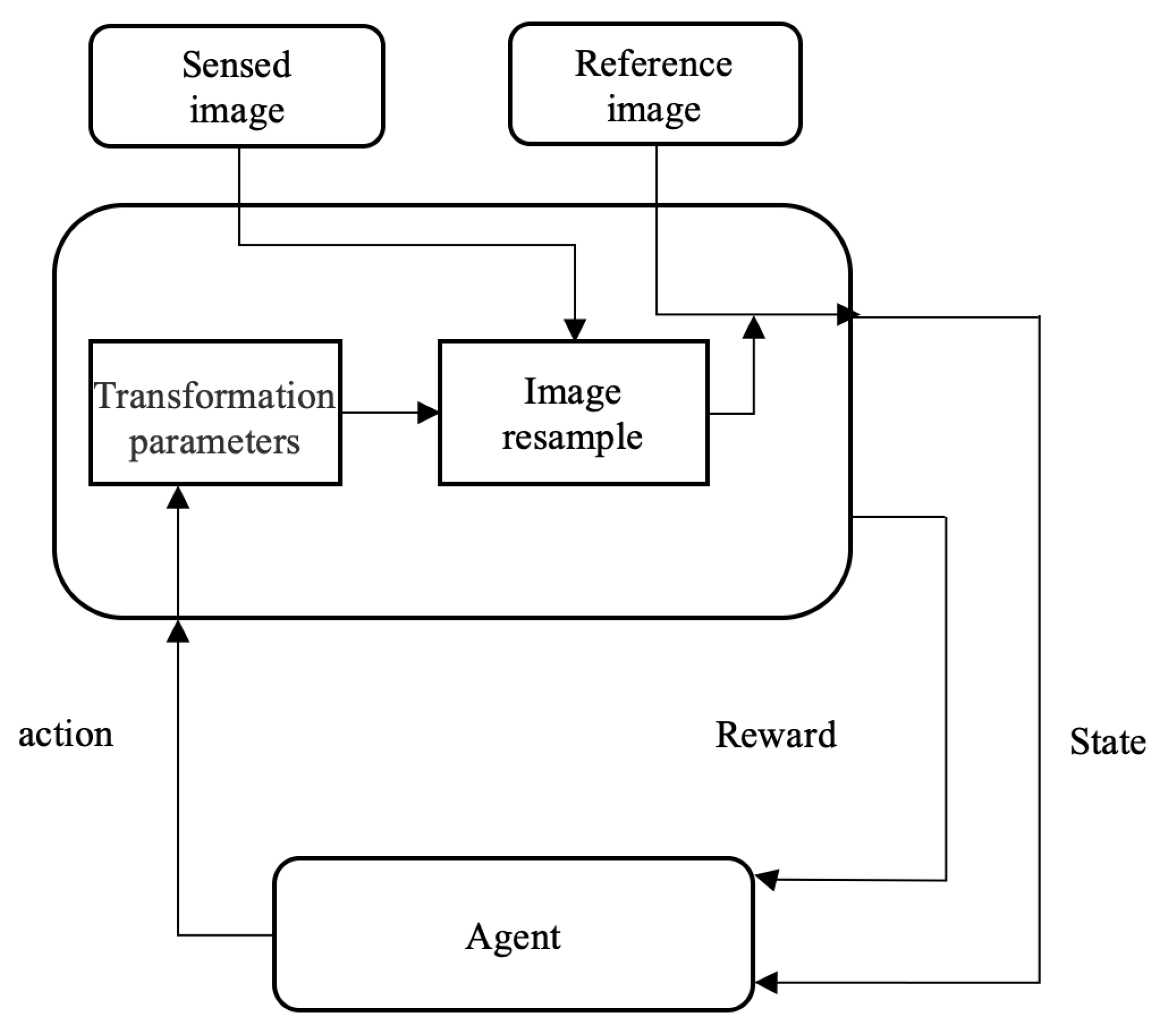
The registration of reference and sensed image pairs is approached as a sequential decision-making process. In this process, the sensed images undergo a transformation based on an action, referred to as a time step, which involves adjusting the transformation parameter. The resulting transformed image, achieved through image resampling, is then registered with the reference image to yield a reward value. This reward value typically indicates whether the latest image resampling has brought the sensed image closer to the reference image. If the transformation executed at that particular time step results in the resampled image being closer to the true value compared to the previous time step, a positive reward is received. Conversely, if the proximity decreases, a negative reward is obtained.

In this research, the state is the grayscale image of the reference and sensed image pairs. The sensed image is resampled according to the affine transformation parameters output by the agent, generating a new sensed image.

The action space consists of the affine transformation parameters of the sensed image, along with an additional trigger action. The agent executes the chosen action, causing the sensed image to undergo the corresponding affine transformation and generating a new sensed image. In this experiment, the discrete action space is defined based on transformation parameters with two scales of low and high precision. This design aims to avoid both registration failures caused by very low precision and high interaction costs resulting from very high precision. The latter scenario might require numerous iterations before achieving a successful registration. The effective action set consists of 16 elements, each corresponding to a specific affine transformation: translate left 1, 10 pixels, translate right 1, 10 pixels, translate up 1, 10 pixels, translate down 1, 10 pixels, rotate clockwise

1^{\circ}

10^{\circ}

, rotate counterclockwise

1^{\circ}

10^{\circ}

, zoom in scale

0.1

0.01

, zoom out scale

0.1

0.01

. The trigger action represents that registration is complete, and further transformations are unnecessary.

The reward function is directly proportional to the enhancement in the alignment of reference and sensed image pairs achieved by the agent through its actions. Intuitively, this improvement can be quantified using the Euclidean distance between the current transformation matrix and the ground truth. However, a challenge arises from differences in parameter units, as the scaling units are smaller compared to translation and rotation. To address this, salient points in the image—such as corner points—are employed to formulate the reward function.

Salient points are identified as key points detected by the maximum value of the Difference of Gaussians (DoG). These key points compose the salient point reference set

P_{G}

, derived from the ground truth of the sensed/reference image. In each training episode, the transform set

{\tilde{P}}_{G}

of salient points is generated by applying the inverse matrix of the transformation matrix.

Subsequently, for each action, the distorted landmarks are transformed using the given transformation matrix. The reward for the action is defined based on the Euclidean distance D between the transformed landmarks and their corresponding landmark references. The entire process is depicted in Figure 1.

3.2. Model

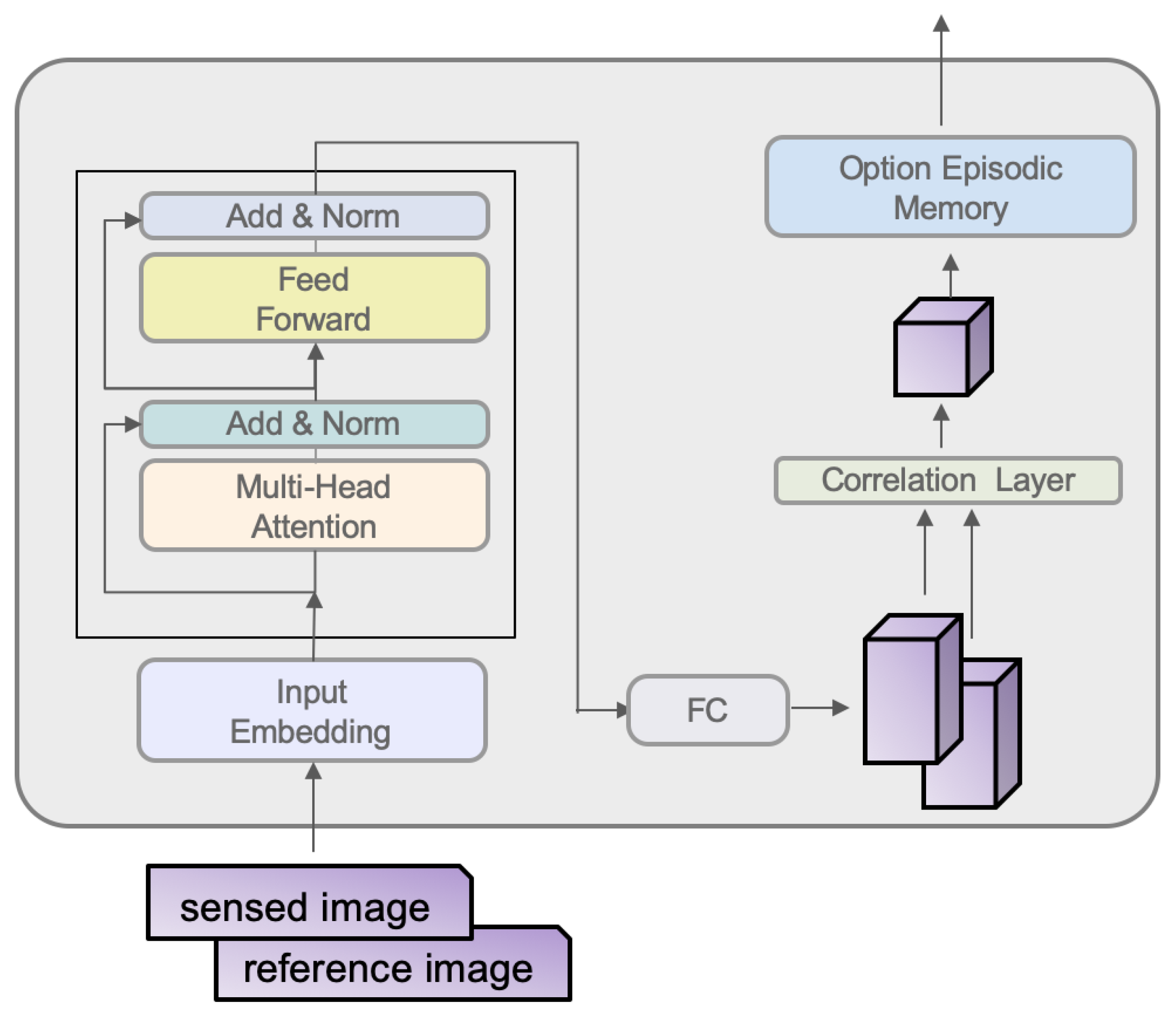
The neural network architecture is illustrated in Figure 2. The left side of the network features a Transformer layer, responsible for conducting feature learning through self-attention on the input sensed and reference image pairs. Meanwhile, the right side of the network comprises a correlation layer that captures position-related details between the sensed and reference image pairs. Ultimately, the network produces the parameters necessary for the affine transformation.

3.2.1. Transformer

The core module of the Transformer is the Multi-Head Attention (MHA). The definition of dot-product attention is as follows:

Attention (Q, K, V) = softmax (\frac{Q K^{T}}{\sqrt{d_{k}}}) V

(1)

Here,

Q \in R^{T \times d_{k}}

is the query matrix,

K \in R^{T \times d_{k}}

is the key matrix, and

V \in R^{T \times d_{k}}

is the value matrix. T and M represent the sequence lengths of queries and keys,

d_{k}

is the feature size of queries and keys, and

d_{v}

is the feature size of V. In visual tasks, Q and K are typically reshaped query and key feature maps, where

T = M = h \times w

, with h and w being the height and width of the feature maps. The definition of Multi-Head Attention is as follows:

{head}_{i} = Attention (Q W_{i}^{Q}, K W_{i}^{K}, V W_{i}^{V})

(2)

MultiHead (Q, K, V) = Concat ({head}_{1}, \dots, {head}_{H}) W^{O}

(3)

where

W_{i}^{Q} \in R^{d \times d_{k}}

W_{i}^{K} \in R^{d \times d_{k}}

W_{i}^{V} \in R^{d \times d_{v}}

, and

W^{O} \in R^{h d_{v} \times d}

are parameter matrices, and H is the number of heads. In the case of the Multi-Head Self-Attention (MHSA) in the encoder,

Q = K = V

The architecture of the Transformer encoder, which excludes positional encoding, is illustrated on the left side of Figure 2. This encoder includes Multi-Head Self-Attention (MHSA) and a feed-forward layer. The feed-forward layer initially increases the feature dimension from d to D and subsequently reduces it back to d. For added depth, the encoder can be stacked a total of N times, where N represents the number of encoder layers. Notably, in this study, a configuration akin to ViT is adopted, employing solely the Transformer encoder and incorporating additional positional encoding.

In the original Transformer design, a decoder with Multi-Head Cross-Attention (MHCA) is employed. Initially, the query consists of a learnable query embedding, which is then replaced by the output of the preceding decoder layer. The key and value components are derived from the outputs of the encoder layers. Similar to the encoder, the decoder can also be stacked N times.

3.2.2. Correlation Layer

The architecture of the correlation layer draws inspiration from the research conducted by Rocco et al. [20]. The objective is to effectively capture both positional and spatial correlation details within image features. The configuration of the correlation layer is depicted on the right side of Figure 2.

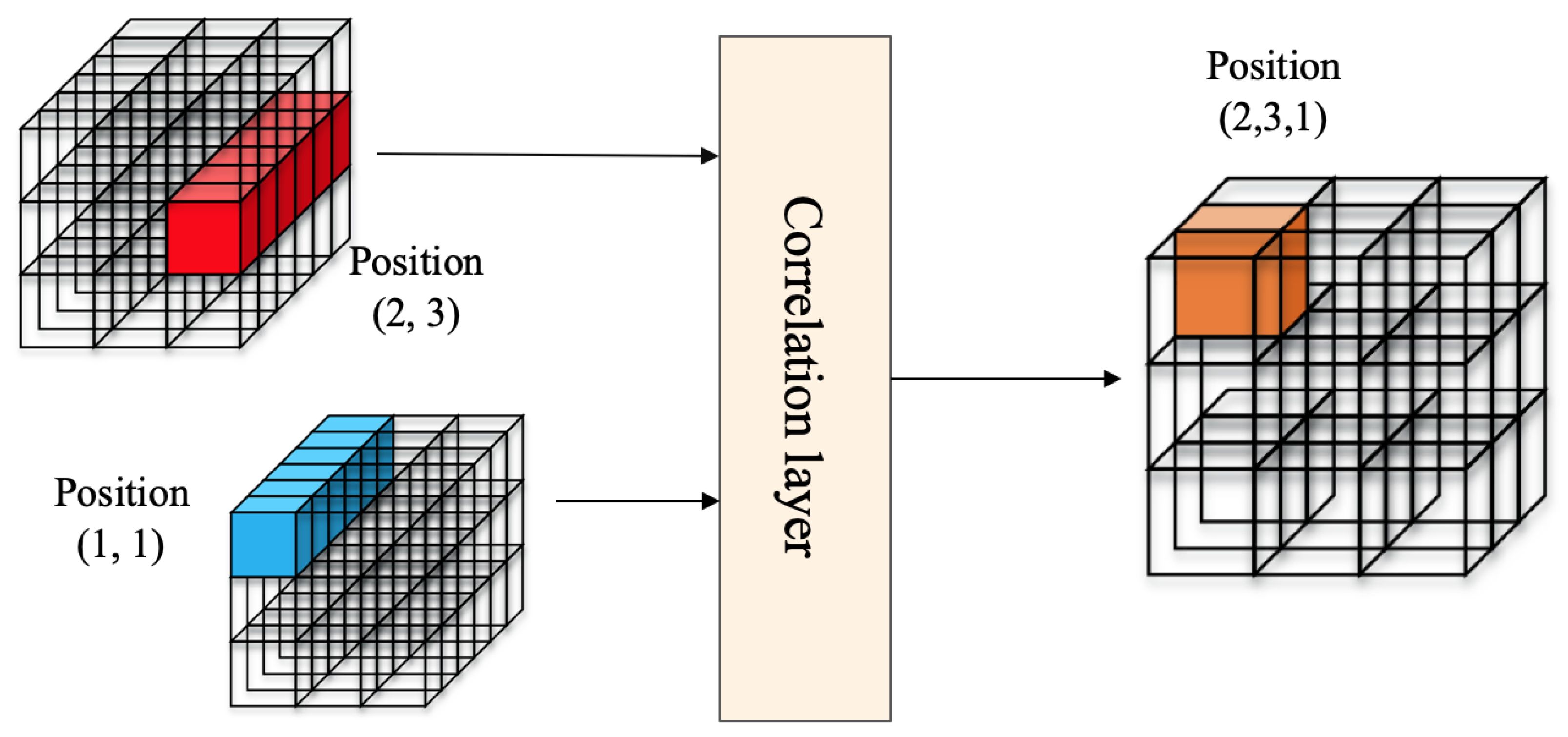
The feature maps

f_{A}

and

f_{B}

are in

R^{h \times w \times d}

, the correlation map

c_{A B}

is in

R^{h \times w \times d}

, and the output of the correlation layer consists of scalar products of individual descriptors at each position:

c_{A B} (i, j, s) = f_{B} {(i, j)}^{T} f_{A} (i_{s}, j_{s})

(4)

(i, j)

and

(i_{s}, j_{s})

represent individual feature positions in the

h \times w

dense feature map, and

s = h (j_{s} - 1) + i_{s}

is an auxiliary index variable for

(i_{s}, j_{s})

The architecture of the correlation layer is illustrated in Figure 3. The right side of the illustration represents the correlation feature

c_{A B}

, which quantifies the similarity between features in

f_{B}

and

f_{A}

at a specific position

(i, j)

. It’s important to emphasize that

c_{A B}

is distinct from

c_{B A}

. The computation of similarity through the correlation feature addresses the challenge of ambiguous matches and necessitates further processing.

To enhance the correlation feature, channel-wise normalization is applied to the correlation feature at each position, yielding a normalized feature

f_{A B}

in the form of a correlation map. Subsequently, Softmax and L2 normalization are employed on the correlation map

f_{A B}

. This normalization approach emphasizes the scores of favorable matches. For instance, when only one feature in

f_{B}

exhibits strong correlation with

f_{A}

, this method resembles nearest-neighbor matching in classical geometry computation [20]. Additionally, in scenarios where descriptors in

f_{B}

match with multiple features in

f_{A}

, resulting from noise or repetitive patterns, the matching scores are down-weighted—a concept similar to the second nearest-neighbor test.

Both the correlation and normalization operations are differentiable in relation to the input features, enabling effective backpropagation for end-to-end learning. Notably, this study employs the self-attention mechanism of the Transformer within the correlation layer to facilitate extensive feature matching across longer ranges.

3.3. Option Episodic Memory

The Option Episodic Memory framework (OptionEM) introduced by Zhou et al. [21] is a comprehensive hierarchical episodic control framework that, to a certain extent, tackles the challenge of extensive sample requirements that posed difficulties for initial generations of deep reinforcement learning models. This framework employs hierarchical episodic memory, updated via implicit memory planning, to estimate the optimal rollout value for each state-action pair.

At each step, the cumulative reward along the trajectory up to that point is compared with the value derived from the memory module. The greater value between these two is chosen. The memory module affiliated with an option encompasses both an option value memory module and an option-internal memory module. The decision regarding which to choose is determined by the termination equation. The notations

M_{θ}

and

M_{Ω, α}

arise from analogous experiences and represent value estimations for counterfactual trajectories linked to options. This process recursively establishes an implicit planning scheme within the episodic memory, aggregating experience longitudinally and across trajectories.

The complete backpropagation process can be formulated using Equation 5.

R_{t} = \{\begin{matrix} r_{t} + γ max (R_{t + 1}, M_{θ} (s_{t + 1}, ω_{t + 1}, a_{t + 1})) & if t < T, β_{ω, η} (s_{t + 1}) = 0 \\ r_{t} + γ max (R_{t + 1}, M_{Ω, α} (s_{t + 1}, ω)) & if t < T, β_{ω, η} (s_{t + 1}) = 1 \\ r_{t} & if t = T \end{matrix}

(5)

where t denotes the step along the trajectory, and T represents the episode length. The backpropagation process in Equation 5 can be expanded and rewritten as Equation 6.

\begin{matrix} V_{t, h} & = \{\begin{matrix} r_{t} + γ V_{t + 1, h - 1} & if h > 0 \\ M_{Ω, α} (s_{t + 1}, ω) & if h = 0, β = 1 \\ M_{θ} (s_{t}, ω_{t}, a_{t}) & if h = 0, β = 0 \end{matrix} \\ R_{t} & = V_{t, h^{*}} \end{matrix}

(6)

where

h^{*} = \underset{h > 0}{arg max} V_{t, h}

Algorithm 1 Update Memory

for stored trajectories $τ$ do
for one of the trajectory $τ$ : $t = T \to 1$ do
according current chosen Option $ω$ ,executing ${\tilde{a}}_{t + 1} \sim π_{ω, θ} (a ∣ s)$
if $β = 0$ then
computing $M_{θ}^{(1, 2)} (s_{t + 1}, ω, a_{t + 1})$
else
computing $M_{Ω, α}^{(1, 2)} (s_{t + 1}, ω)$
end if
for $h = 0 : T - t$ computing $V_{t, h, ω}^{(1, 2)}$ according (5)
computing $R_{t, h, ω}^{(1, 2)}$ according (6)
saved into the memory
end for
end for

The parameterized neural network

M_{θ}

is introduced to represent the parameterized option-internal memory, while the parameterized neural network

M_{α}

serves as the parameterized option memory. Both networks are learned from a tabular memory M. In order to harness the generalization capability of

M_{θ}

and

M_{α}

, an augmented reward is propagated along trajectories using value estimates from

M_{θ}

and

M_{α}

, along with the actual rewards from M. This approach aims to determine the optimal value across all potential rollouts. During training, the improved target is regressed to train the versatile memories

M_{θ}

and

M_{α}

, with the chosen value guided by the termination equation. This refined target then guides policy learning and establishes fresh learning objectives for OptionEM.

A key challenge within this learning process is the potential overestimation stemming from identifying the best value along a trajectory. During the backpropagation process, overestimated values can persist and hinder efficient learning. To mitigate this challenge, a Siamese Network, akin to the concept of Double Q-learning, is employed to refine the backpropagation of value estimates. Traditional reinforcement learning algorithms with function approximation are prone to overestimating values, which makes addressing this tendency critical. The Siamese Network structure is leveraged to render value estimates from

M_{θ}

more conservative. Training involves updating the memory network, the termination function, and the option policy using three distinct timescales.

Algorithm 2 Option Episodic Memory(OptionEM)

Initializes the episodic memory network and option network
Initializes the target network parameters $θ_{(1)}^{'} \leftarrow θ_{(1)}, θ_{(2)}^{'} \leftarrow θ_{(2)}, α_{(1)}^{'} \leftarrow α_{(1)}, α_{(2)}^{'} \leftarrow α_{(2)}, ϕ^{'} \leftarrow ϕ, ζ^{'} \leftarrow ζ, η^{'} \leftarrow η$
Initializes the episodic memory $M$
for $t = 1, . . ., T$ do
Choose Option $ω$ ,execute action a
receive reward r and next state $s^{'}$
store tuple $(s, ω, a, r, s^{'}, ω^{'}, β)$ in memory $M$
for $i i n {1, 2}$ do
sample N tuples $(s, a, r, s^{'}, β, R_{t}^{i})$ from memory $M$
if $β = 0$ then
update $θ_{(i)} \leftarrow {min}_{θ_{(i)}} \sum {(R_{t}^{(i)} - M_{θ}^{i} (s, ω, a))}^{2}$
else
update $α_{(i)} \leftarrow {min}_{α_{(i)}} \sum {(R_{t}^{(i)} - M_{α}^{i} (s, ω))}^{2}$
end if
end for
if $t m o d u = 0$ then
$θ_{(i)}^{'} \leftarrow τ θ_{(i)} + (1 - τ) θ_{(i)}^{'}$
$α_{(i)}^{'} \leftarrow τ α_{(i)} + (1 - τ) α_{(i)}^{'}$
$η_{(i)}^{'} \leftarrow τ η_{(i)} + (1 - τ) η_{(i)}^{'}$
$ϕ_{(i)}^{'} \leftarrow τ ϕ_{(i)} + (1 - τ) ϕ_{(i)}^{'}$
update Episodic Memory according Algorithm 1
end if
if $t m o d p = 0$ then
update $ϕ$ , $\nabla_{ϕ} J (ϕ) = {\nabla_{a} M_{θ_{1}} (s, ω, a)|}_{ω = π_{ω}, a = π_{ϕ} (s)} \nabla_{ϕ} π_{ϕ (s)}$ according policy gradient
update $ζ$ , $\nabla_{ζ} J (ζ) = {\nabla_{ω} M_{α_{1}} (s, ω)|}_{ω = π_{ω}} \nabla_{ζ} π_{ζ (s)}$ according policy gradient
end if
if $t m o d q = 0$ then
update $η$ , $\frac{\partial M_{α} (ω_{0}, s_{1})}{\partial η} = - \sum_{s^{'}, ω} μ_{Ω} (s^{'}, ω ∣ s_{1}, ω_{0}) \frac{\partial β_{ω, η} (s^{'})}{\partial η} A_{Ω} (s^{'}, ω)$ according policy gradient
end if
end for

3.4. Self-Learning

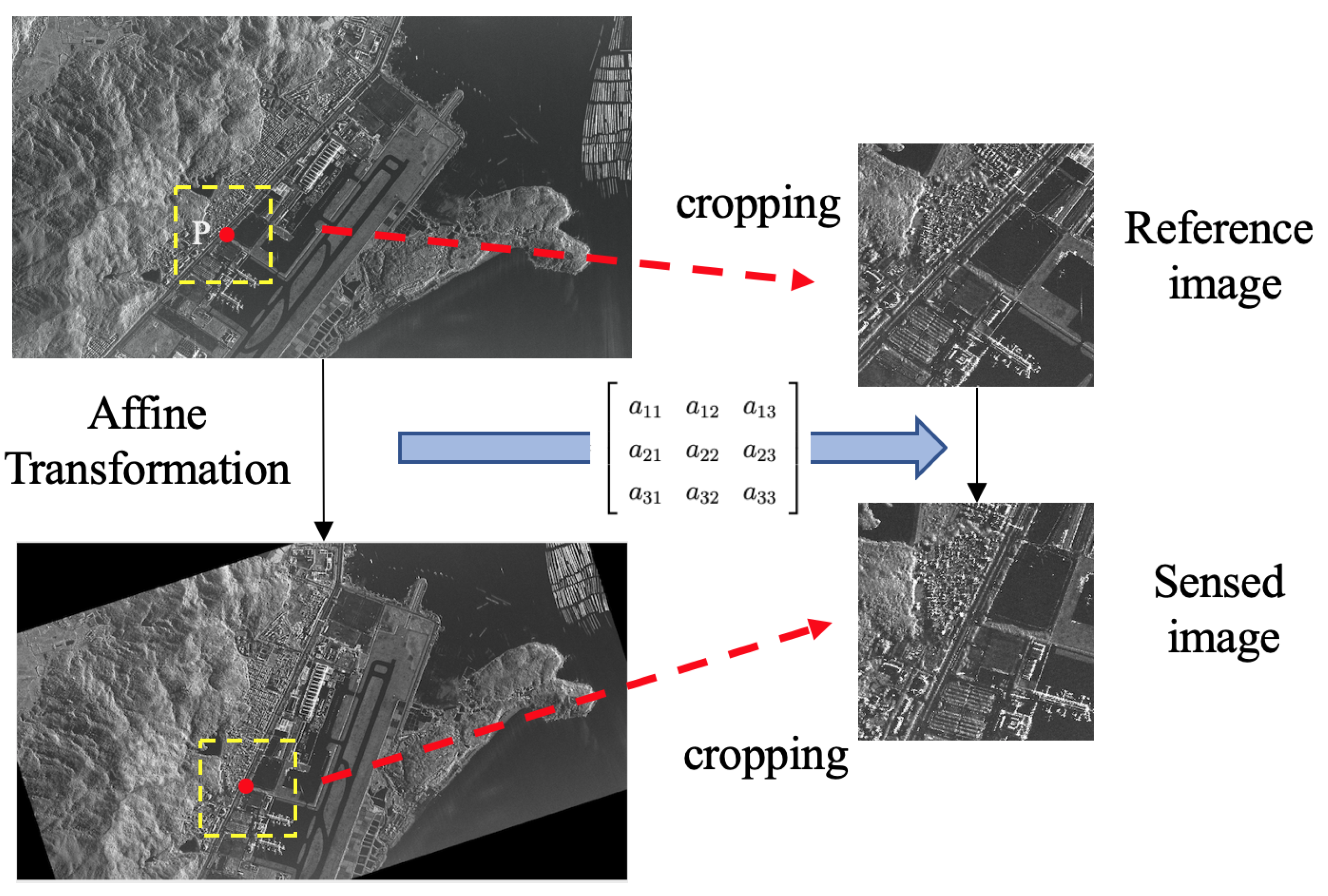
Compared to RGB image datasets, SAR image datasets are relatively limited in availability, and acquiring labeled datasets can be expensive. To tackle this challenge, this study employs a self-learning strategy. The core concept is to apply various transformation matrices—like translation, scaling, rotation, etc.—to images. Consequently, a substantial number of corresponding sensed and reference image pairs are generated from the original images and their transformed versions. In the context of SAR image registration, the training dataset can be produced by applying affine transformations to one of the image pairs.

In this scenario, the initial large-scale image undergoes an affine transformation. A

240 \times 240

pixel image patch is selected from the original image as the reference image. Utilizing the coordinates of the reference image’s center point within the original image, the coordinates for this point are calculated within the transformed large-scale image using the transformation matrix. Subsequently, a

240 \times 240

pixel image patch is cropped to serve as the sensed image, with its center point determined by the computed coordinate values. This self-learning approach eliminates image patches that might exhibit black boundaries after the image patch’s affine transformation, ensuring dataset quality. The process of self-learning is visually represented in Figure 4.

This self-learning strategy proves effective in alleviating the need for extensive sample data. Shuang Wang et al.’s work has already illustrated the method’s success in SAR image registration through a deep learning framework [2]. However, their primary objective was to acquire localized feature information and details about feature point neighborhoods. To achieve this, they harnessed self-learning to generate a significant quantity of sample data, focusing on feature points and their surrounding localized information.

In contrast, this current study employs self-learning to create an extensive amount of global sample data. The self-learning samples are designed to construct new sensed-reference image pairs on a larger scale, rather than primarily concentrating on localized feature points.

4. Experiments

4.1. Dataset

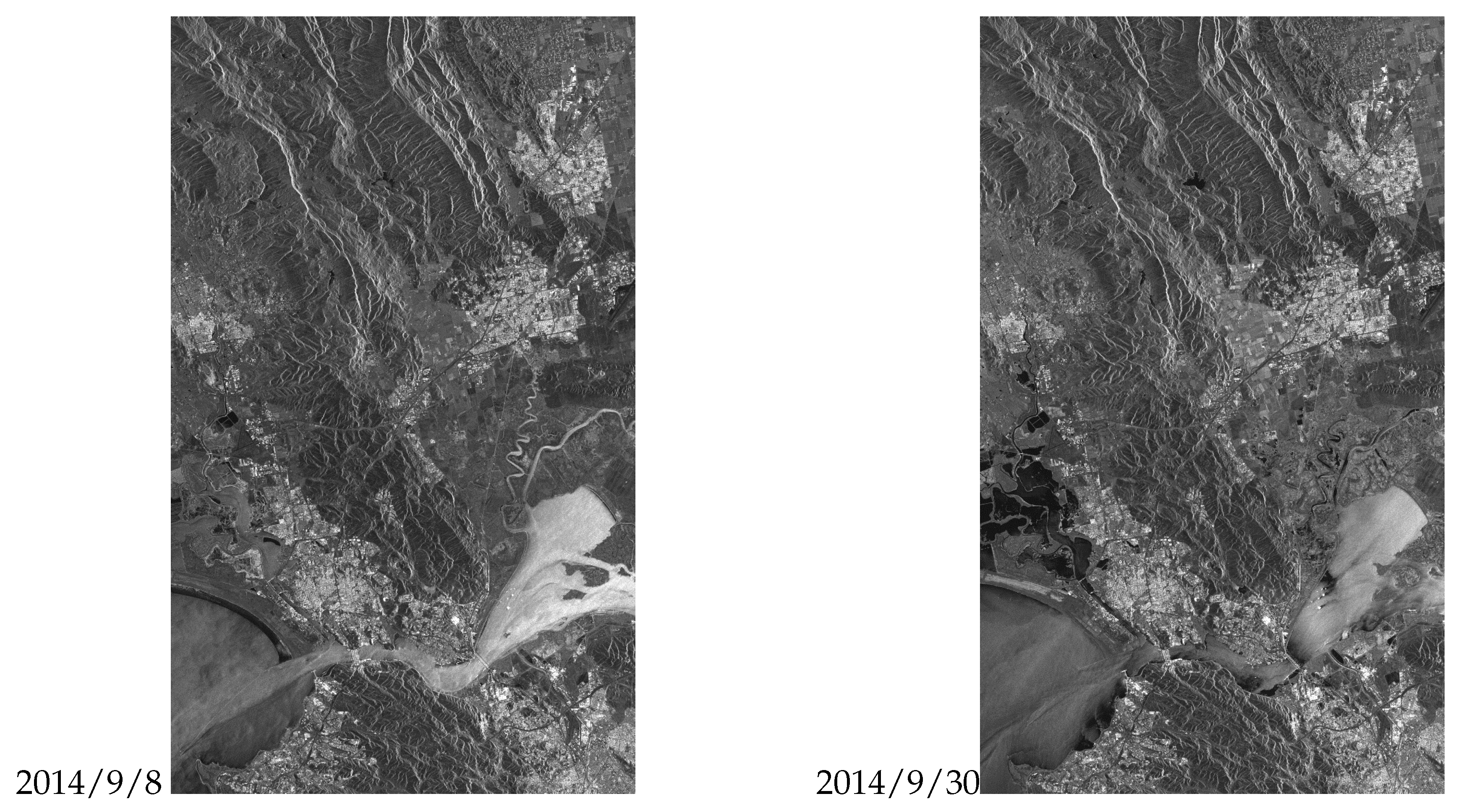
The training image dataset for this experiment was generated using the right-looking descending image from the TerraSAR-X satellite over Napa, USA.1. These images were captured on September 8 and September 30, 2014, respectively, as depicted in Figure 5. By observing the images, evident changes in grayscale and coverage can be noticed, particularly over the water bodies. It’s essential to recognize that the presented images are quick-look previews, which are scaled-down versions of the original full-scene images. The resolution of these previews is approximately ten times smaller than that of the actual data.

In comparison to the SAR image taken on September 30, the SAR image captured on September 8 exhibits an offset of approximately 60 pixels in the range direction. The SAR reference image utilized during the network training phase is derived from a pre-processed version of the original image taken on September 30, 2014.

Due to the substantial size of SAR images and their inherent characteristics, including speckle noise and geometric distortions, a series of preprocessing steps are applied to the original images. These steps encompass block division, multilook, filtering, downsampling, and differencing.

Acquiring a significant volume of annotated remote sensing images, as opposed to optical image datasets, poses challenges due to the specialized domain knowledge required and the associated costs. To address this challenge, a self-learning strategy is employed. Given that SAR images can be captured under diverse conditions—such as varying incidence angles, distinct orbital directions, and diverse azimuth angles—various fundamental transformation types are employed for the affine transformation of the reference image. These fundamental transformations include translation, scaling, rotation, and flipping. This approach aims to examine the resilience of image features to these core transformation types. The parameters for these transformations are uniformly sampled within predefined ranges, and each affine transformation is created by combining these fundamental transformations.

Once the training dataset comprising sensed and reference image pairs is generated, SAR images undergo standardization and normalization. Image standardization, a widely used preprocessing technique, involves centering the data by subtracting the mean. This alignment with convex optimization theory and knowledge about data probability distribution enhances the suitability of the centered data distribution for generalization after training. Standardization results in a zero-mean centered data distribution, enhancing the effectiveness of gradient descent algorithms. Furthermore, it eliminates common image characteristics while accentuating individual differences. As a result, neural networks can learn more distinctive features, thereby fostering rapid learning, iteration, optimization, and improved learning efficiency. In this experiment, standardization parameters mean and standard deviation are set to

m e a n = 0.485

and

s t d = 0.229

For generating training data, 60 small images of size

240 \times 240

pixels are cropped from the larger source image. Each of these small images undergoes 700 affine transformations. The scaling factor ranges from

0.71

1.5

(uniformly sampled), and the rotation angle spans from

- 180

to 180 degrees with a precision of 1 degree (uniformly sampled). No flipping transformations are applied.

In this paper, we utilize three distinct datasets for testing:

1. TerraSAR-X Napa 2014 Dataset: Already introduced in the training dataset section, consisting of 110 pairs of

240 \times 240

pixel image blocks.

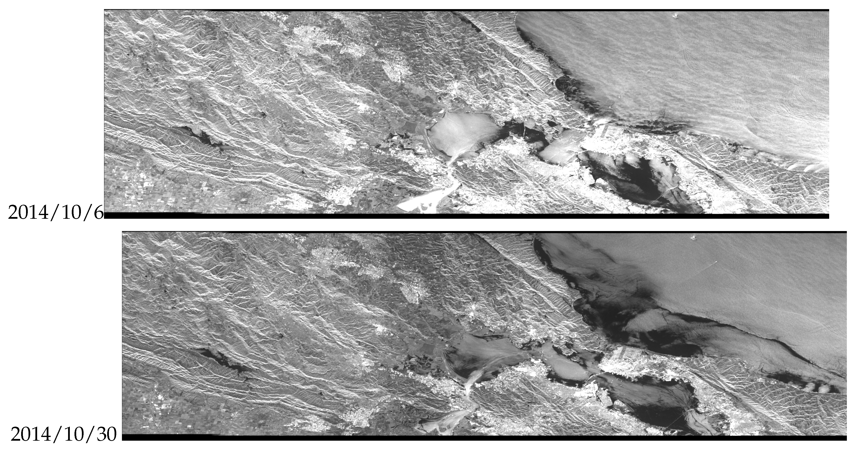
2. Sentinel-1A Napa 2014 Dataset: Source images are obtained from Sentinel-1A SAR satellite images of the Napa region in the western United States on October 30th and October 6th, 2014. A total of 18 pairs of

240 \times 240

pixel image blocks were cropped.

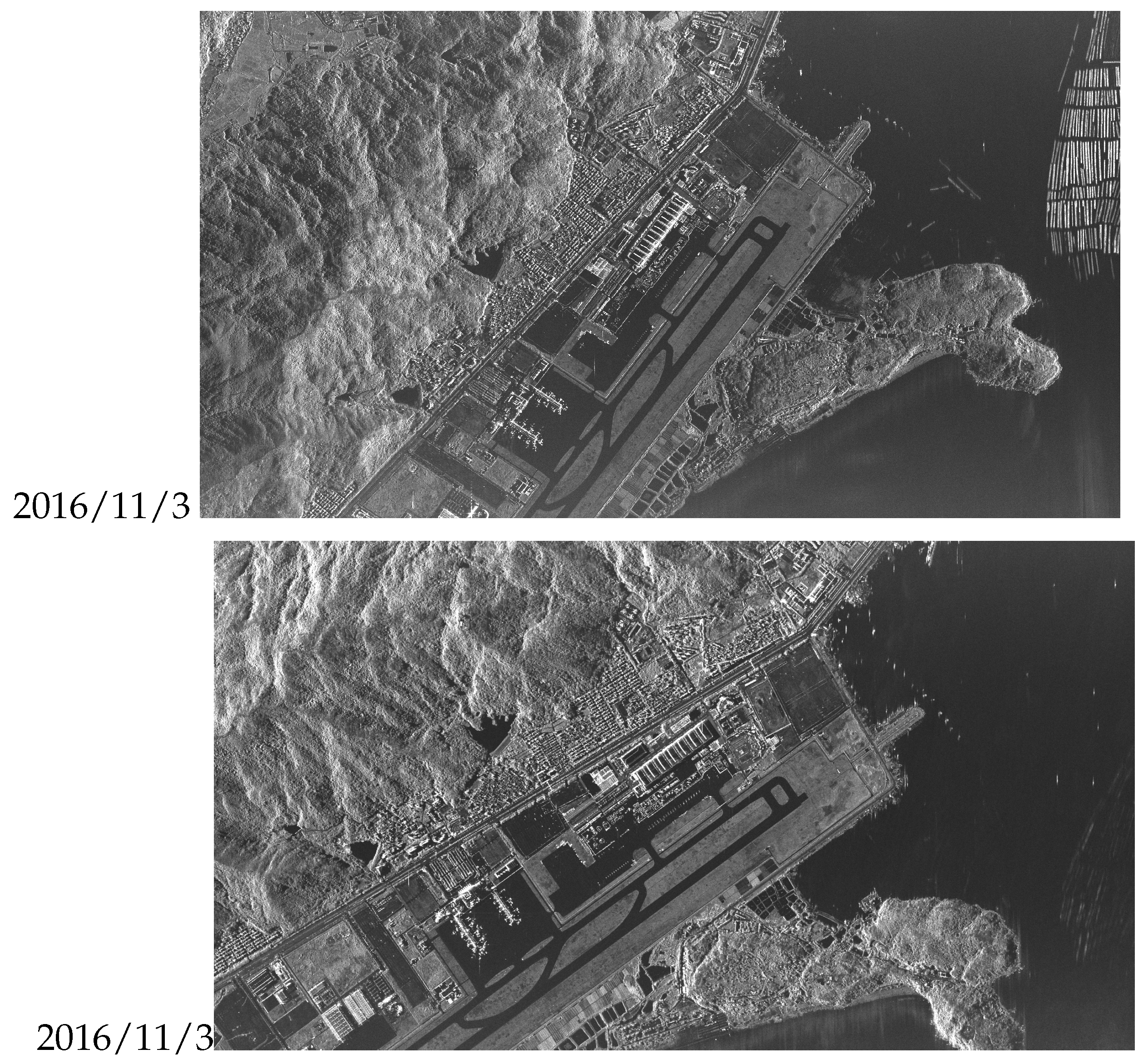
3. TerraSAR-X Zhuhai 2016 Dataset: Source images are obtained from TerraSAR-X satellite images of the Zhuhai region in southern China, captured on November 3rd, 2016. A total of 62 pairs of

240 \times 240

pixel image blocks were cropped.

Figure 6. Descending pass right-looking SAR images from different periods of the Sentinel-1A satellite over the Napa region, USA.

Figure 7. Right-looking SAR images from the TerraSAR-X satellite over Zhuhai region, China. (a) Descending pass (b) Ascending pass.

The initial test dataset employs original images that align with the training dataset. Given the relative consistency in the imaging geometry of SAR sensed and reference images—featuring minor variations in geometric structural characteristics—the evaluation of the proposed registration method’s resilience to translation, scale, rotation, and other geometric transformations necessitates the application of random affine transformations to the SAR sensed images. The types of transformations and the parameter ranges used for preprocessing remain consistent with those applied to the training dataset. Notably, the preprocessing methods employed across all three sets of test data are identical.

It is evident that the Sentinel-1A Napa 2014 image dataset contains more noise and pronounced dissimilarities in image features—such as water bodies and ridges—when contrasted with the training dataset derived from TerraSAR-X Napa 2014. Furthermore, the brightness distribution of images demonstrates considerable variations. Conversely, the TerraSAR-X Zhuhai 2016 dataset displays a greater presence of linear features, and its overall brightness distribution closely resembles that of the TerraSAR-X Napa 2014 dataset.

4.2. Option Analysis

Table 1 illustrates the correlation between Normalized Root Mean Square Error (RMSE) and Options. An option is displayed when the occurrence probability surpasses

75 %

within the RMSE range of statistically distinct score intervals across the three test datasets. Conversely, it is denoted as ’-’ when the option’s proportion falls within the range of

25 % - 75 %

. For instance, consider the TerraSAR-X Zhuhai 2016 dataset, which consists of 62 pairs of test sets. In the testing process, among 238 instances of image pairs with normalized RMSE in the range

[0, 0.2)

, the agent chose option 0 a total of 223 times, resulting in a proportion of

193 / 238 = 93 %

. Therefore, in the table, it appears as option 0. On the other hand, for 502 image pairs with normalized RMSE in the range

[0.4, 0.6)

, the agent selected option 0 in 337 cases, accounting for a proportion of

337 / 502 = 67 %

. Consequently, this is indicated as ’-’ in the table.

The data implies that across the three test datasets, the agent is more inclined to opt for fine registration when the option is 0, while it tends to select coarse registration when the option is 1. Notably, the complexity of the data in the Sentinel-1A Napa 2014 dataset results in unstable performance. Subsequent experimental results demonstrate that this dataset yields poorer registration outcomes relative to the other two test datasets.

It’s important to highlight that there exist numerous metrics for measuring image pair similarity, with Root Mean Square Error (RMSE) being a straightforward indicator. However, RMSE’s emphasis on pixel-level discrepancies can lead to challenges when assessing SAR image pairs, which may exhibit significant differences in scale, noise, grayscale, structural features, and more, thereby substantially influencing the accuracy of RMSE.

Indeed, there are instances where image pairs might share similar grayscale values but fail to match in other aspects [2]. Moreover, the root mean square error can also be influenced by factors like the quantity, distribution, and precision of the feature point pairs. The examples provided in this section serve the purpose of illustrating the general connection between image disparities and options. However, it’s crucial to note that these examples do not constitute quantitative analyses.

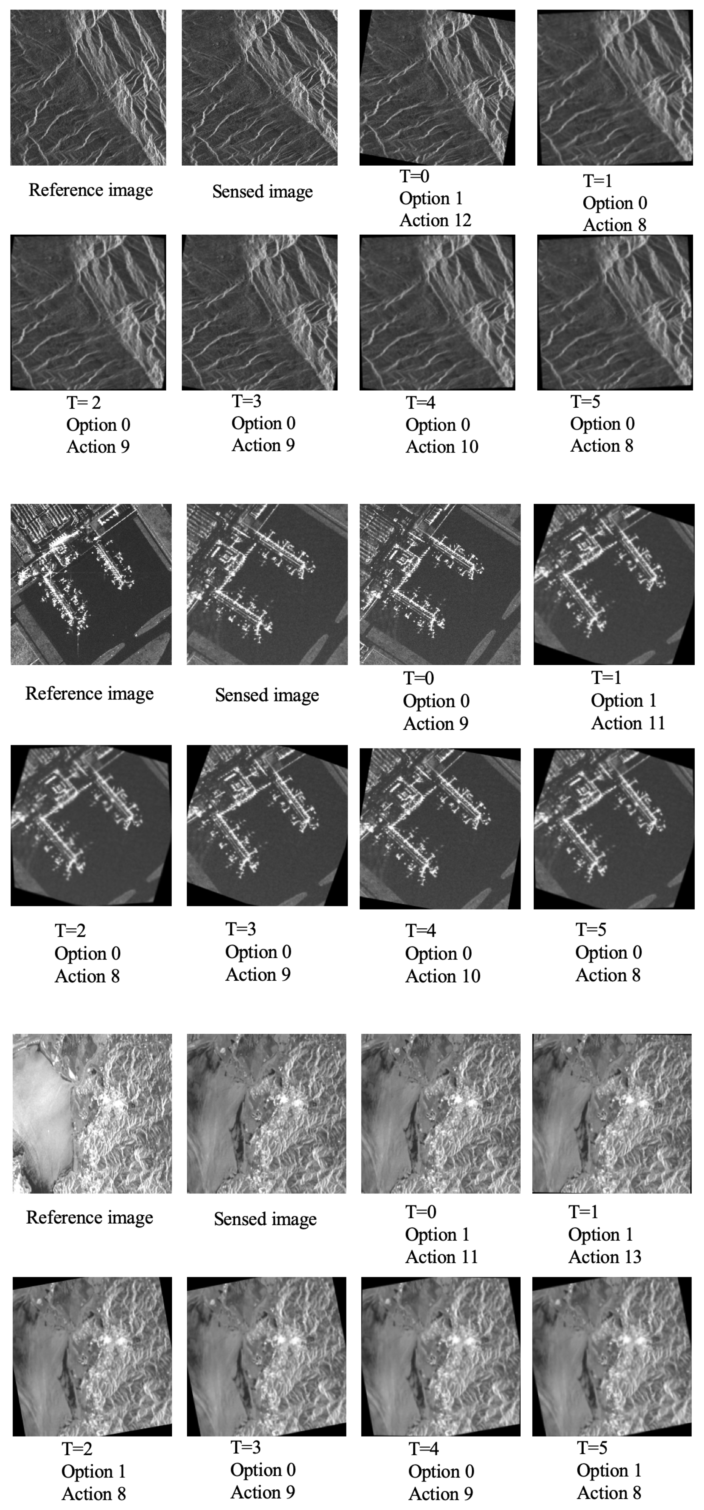
Figure 8 visually portrays the registration process of three image pairs, offering a comprehensive view of the reinforcement learning-based registration method’s entire path and more intuitively showcasing the option strategy employed throughout the registration process.

An observation can be made that even in cases where a large difference exists between the sensed image and the reference image—such as the

T = 0

timestep in the second image pair—the occurrence of option 0 does not adversely impact the subsequent registration process. Across the first and second image pairs, the agent tends to favor the selection of the coarse registration option, involving significant rotation (e.g., the

T = 0

timestep in the first image pair and the

T = 1

timestep in the second image pair). Subsequently, the agent executes scaling and rotation to achieve fine registration (e.g.,

T = 1, 2, 3, 4, 5

timesteps for the first image pair and

T = 2, 3, 4, 5

timesteps for the second image pair).

In the case of the third image pair, the agent’s decision-making process appears to exhibit some instability (e.g., the

T = 5

timestep). However, it’s worth noting that the outputs for the

T = 1, 2, 3

timesteps align with expectations, indicating a certain level of consistency.

4.3. SAR Image Registration Results Analysis

4.3.1. Once-Registration and Re-registration

In this study, we introduced a comprehensive image registration approach that delivers the affine transformation matrix and registered images directly from input sensed and reference images. Unlike methods with distinct stages like feature point extraction, direction assignment, and descriptor construction, our algorithm doesn’t offer a direct calculation of quantitative measures relying on feature points.

To enable a meaningful comparison with conventional registration techniques, we devised an indirect strategy. This approach involves two steps: first, the initial registration of sensed and reference images; and second, a subsequent re-registration wherein the sensed image is registered with the SAR-RL (Reinforcement Learning) registered image. Quantitative metrics are then computed for both scenarios. The underlying assumption is that if the re-registration outcome exhibits a smaller Root Mean Square Error (RMSE) value and elements of the affine transformation matrix that are closer to zero, it implies an improved SAR-RL registration result, in line with expectations.

4.3.2. Qualitative Evaluation Results

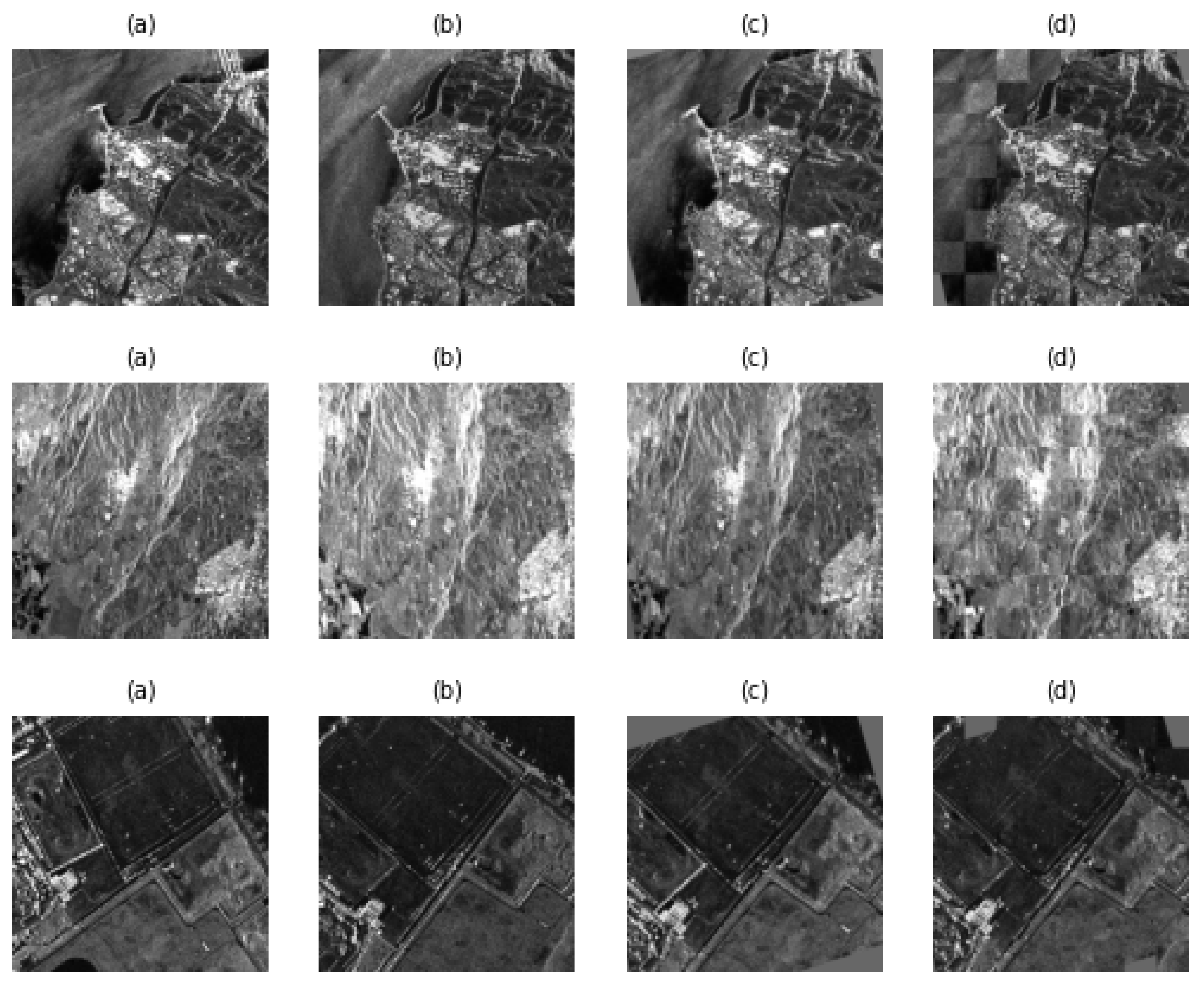
The qualitative assessment primarily involves visually inspecting the spatial geometric registration results of the registered images [2]. This can be achieved by overlaying the registered reference image onto the sensed image using distinct colors to gauge the extent of overlap and differences in content. Another technique involves dividing the images into smaller blocks and overlapping them in a checkerboard pattern to create a mosaic map. By examining the continuity of structural features (such as stitching boundaries, rivers, bridges, roads, ridges, etc.) and assessing the overlap of common areas, the effectiveness of registration can be assessed. While this approach is straightforward and effective, it might not be suitable for large-scale automated applications.

Figure 9 provides examples of checkerboard-mosaicked images for the three test datasets. Due to space limitations, one example is selected from each dataset: a land-water interface area containing man-made structures and mountains, a mountainous region, and an airport area. As evident from column d in the figure, the sensed images and reference images from the three scene sets demonstrate successful registration. Most regions of the images overlap well, and the stitching boundaries are consistent.

Furthermore, it’s noticeable from columns d and c that the sensed images produced by the SAR-RL technique exhibit a high visual similarity to the reference images in terms of geometric structural features. This aspect lays the groundwork for achieving effective registration.

4.3.3. Quantitative Evaluation Results

Quantitative evaluation involves expressing registration outcomes in numerical terms. Commonly employed metrics for quantitative assessment encompass the count of control point pairs (

N_{r e d}

), the Root Mean Square Error (RMSE) of all control point residuals (

R M S E_{a l l}

), and RMSE calculated using the leave-one-out method (

R M S E_{L o o}

). These metrics are frequently normalized to the pixel size to facilitate comparisons [22].

The transformation matrix (T) for control point pairs is determined through the least squares method, and based on this matrix, the residuals of control point pairs are computed, giving rise to

R M S E_{a l l}

and

R M S E_{L o o}

. The presence of more accurately matched point pairs translates to a better determination of the parameters in the geometric transformation model, thereby yielding enhanced performance [12]. However, it’s important to note that an increase in the number of correctly matched point pairs acquired through a registration method doesn’t necessarily guarantee a decrease in the Root Mean Square Error. This is because errors can still persist in the point pairs matched by the algorithm.

Gonçalves et al. took into account the distribution of control points and residuals and put forward various evaluation metrics, which include the quadrant residual distribution (

P_{q u a r d}

), the proportion of poorly matched points with residuals (norm) exceeding 1.0 (Bad Point Proportion, BPP) denoted as BPP(1.0), the detection of a preferred axis in the residual scatter plot (

S_{k e w}

), the statistical attributes of control point distribution in the image (

S_{c a t}

), all of which were considered in conjunction with

N_{r e d}

R M S E_{a l l}

, and

R M S E_{L o o}

. Among these metrics, except for

N_{r e d}

, smaller values in the other evaluation metrics signify improved registration performance [2].

These seven metrics are not completely independent of one another. For instance, a higher value of

N_{r e d}

along with a lower value of

R M S E_{a l l}

indicates greater accuracy in point matching. Conversely, if both metrics are either high or low, it suggests lower accuracy.

In order to compare our method with traditional and deep learning-based approaches, we have selected SAR-SIFT and Wang Shuang’s research (referred to as DL-WangS) [2] as benchmarks. Figure 10, Figure 11 and Figure 12 illustrate the interval statistical results of Root Mean Square Error (RMSE) values for SAR-SIFT, DL-WangS [2], and our re-registration results for the three datasets.

The intervals depicted in these figures are

[0, 0.01)

[0.01, 0.1)

[0.1, 0.2)

[0.2, 0.3)

[0.3, 0.4)

[0.4, 0.5)

[0.5, 0.6)

[0.6, 0.7)

[0.7, 0.8)

[0.8, 0.9)

[0.9, 1)

, and

[1, \infty)

These can be seen in the figures , the re-registration results after the initial registration of sensed and reference image pairs used for testing are significantly better. Results from the TerraSAR-X Napa 2014 dataset and TerraSAR-X Zhuhai 2016 dataset outperform those from the Sentinel-1A Napa 2014 dataset. About

24 %

of re-registrations in the TerraSAR-X Napa 2014 dataset achieved RMSE values below

0.01

, while only

5 %

in the Sentinel-1A Napa 2014 dataset achieved this. Similarly,

24 %

of re-registrations in the TerraSAR-X Zhuhai 2016 dataset achieved RMSE values below

0.01

. The RMSEs obtained by SAR-SIFT are concentrated around 1 pixel, with a small portion larger than 1 pixel. The RMSEs obtained by DL-WangS are mostly smaller than 0.6 pixel, but for the Napa region images, some are close to 1 pixel. The RMSEs obtained by our proposed re-registration method are all less than 1 pixel and are concentrated near 0. This suggests that our re-registration achieves sub-pixel level accuracy and outperforms SAR-SIFT, while being comparable or even slightly better than DL-WangS.

Table 2 and Table 3 present the median and mean values of the quantitative analysis results for SAR-SIFT, DL-WangS [2], and our SAR-RL model after re-registration applied to the three datasets. The analysis is conducted using the seven metrics introduced by Gonçalves et al. (2009) to quantitatively evaluate the registration results for all image pairs in the test datasets.

Comparing and analyzing the quantitative results in these tables, several observations can be made: The

N_{r e d}

value obtained by re-registration is comparable to that of SAR-SIFT, indicating that a similar number of control point pairs are correctly matched. However, our re-registration achieves more accurate registration results. The

N_{r e d}

value obtained by re-registration is lower than that of DL-WangS, but the accuracy achieved is comparable. The

S_{c a t}

value obtained by re-registration is comparable to that of both SAR-SIFT and DL-WangS, suggesting that the distribution of matched feature point pairs obtained by the three methods is similar. It can also be observed that the running time of SAR-SIFT is in the order of tens of seconds, while DL-WangS takes seconds to run. In contrast, our re-registration method has a significantly faster registration speed, with running times in the sub-second range.

These tables provide a comprehensive overview of the quantitative evaluation results and highlight the strengths of our re-registration method in terms of accuracy and efficiency compared to the other methods.

It should be emphasized that the re-registration approach does not directly measure the performance of the SAR-RL method. The calculation of metrics still relies on the SIFT and SAR-SIFT algorithms. However, the metrics indicate that SAR-RL registration is significantly more accurate than these two traditional methods.

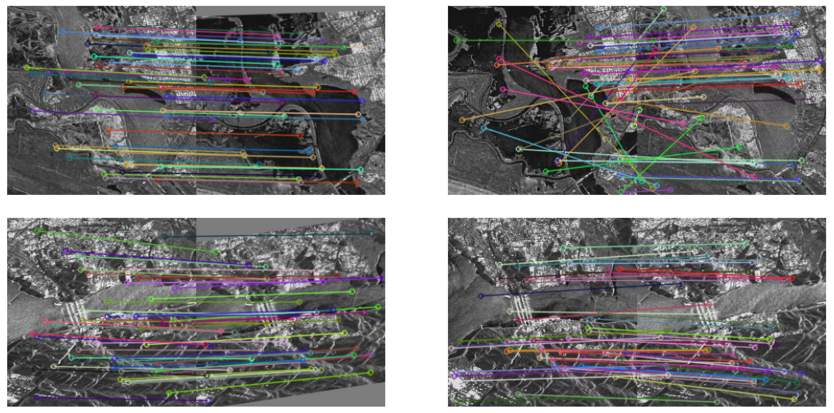
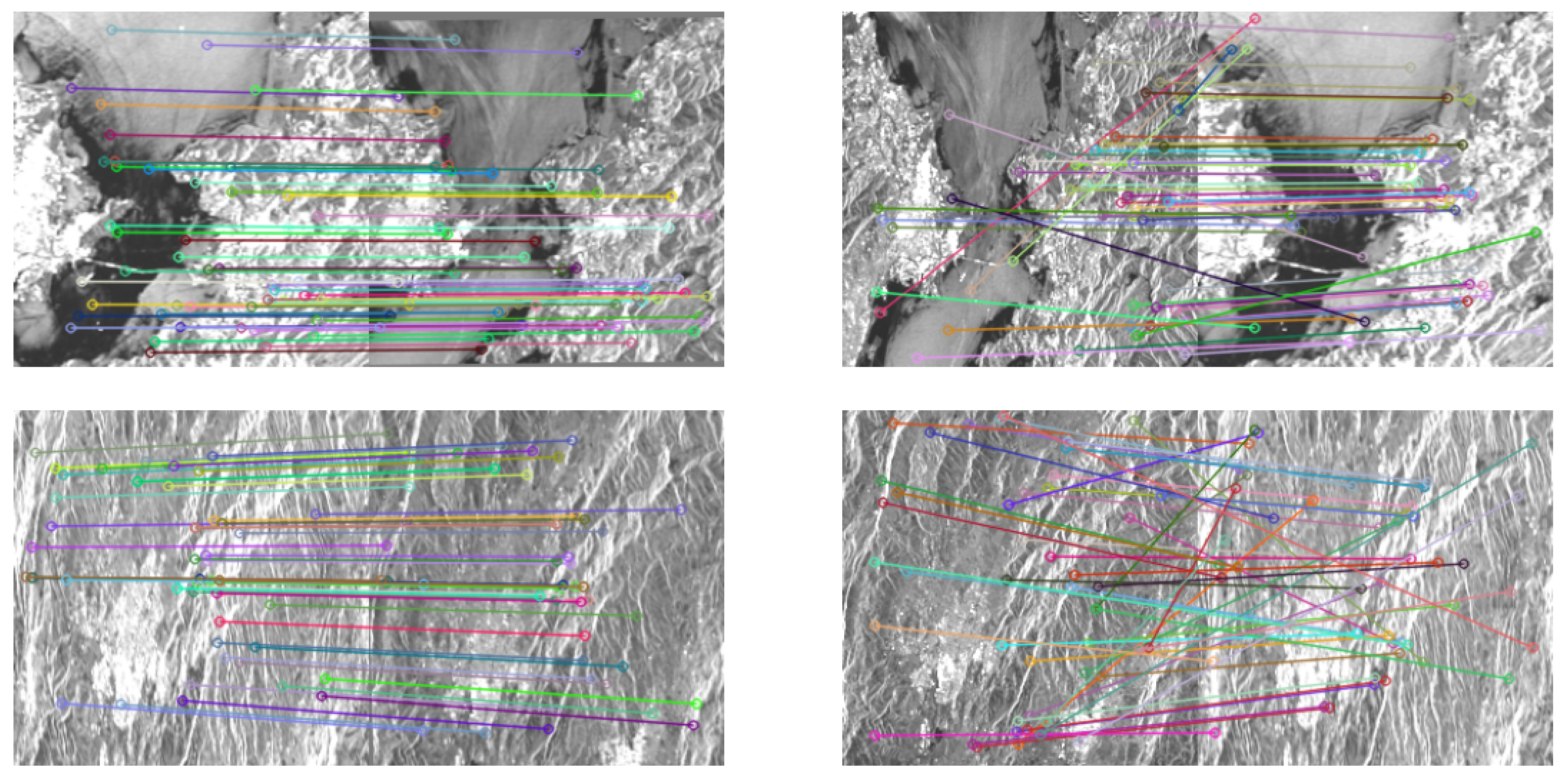
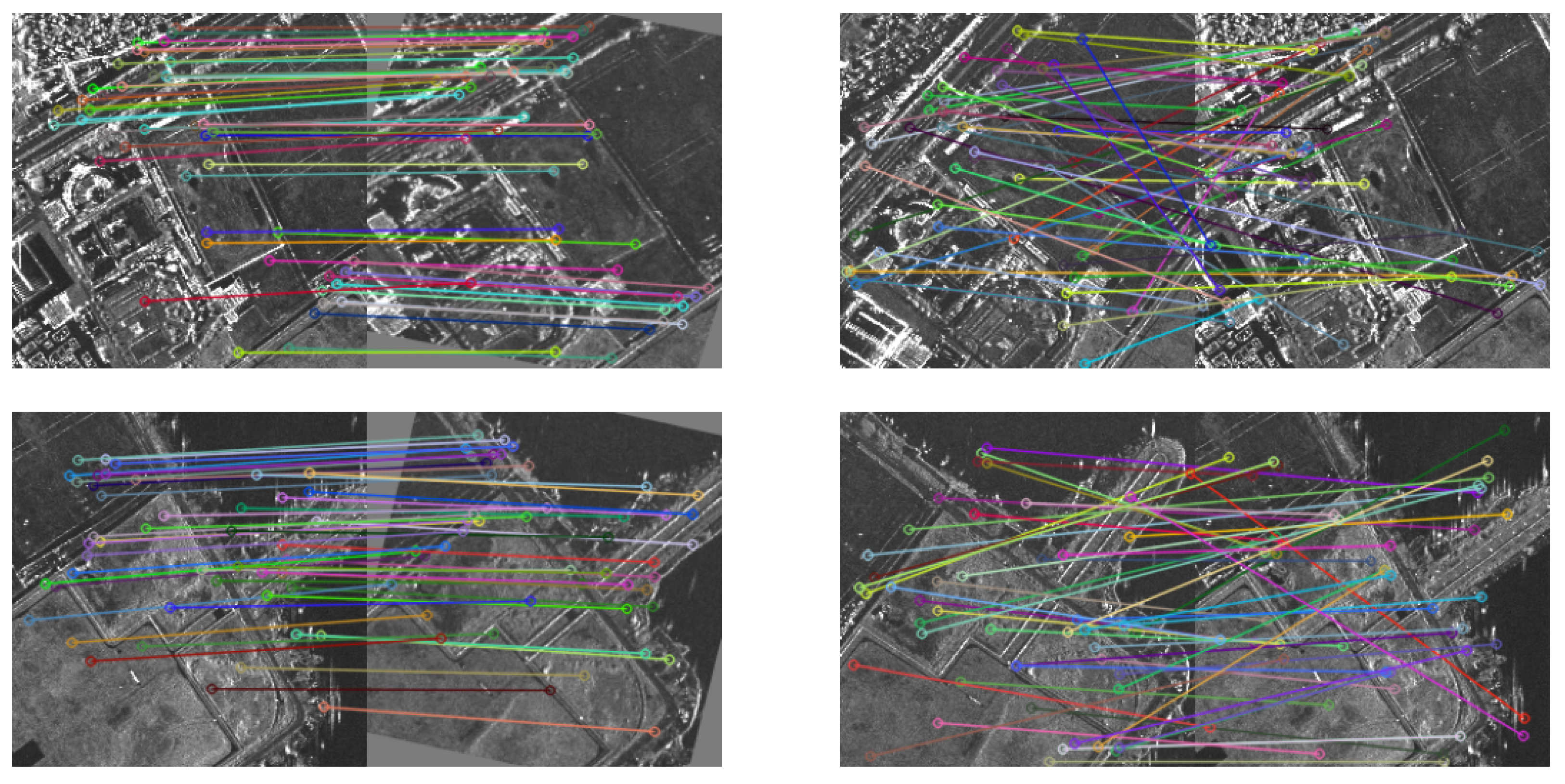
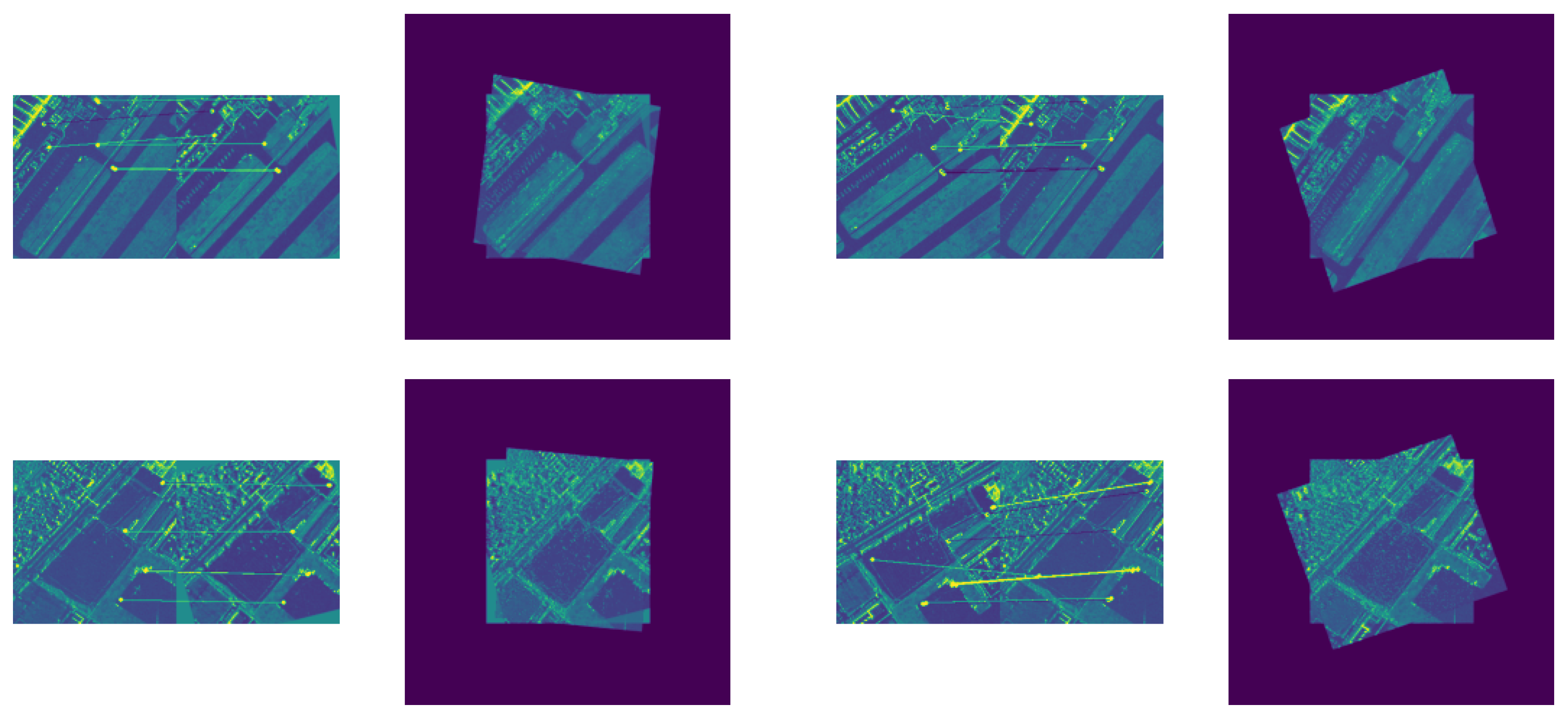
The visual comparisons we’ve provided through Figure 13, Figure 14 and Figure 15 effectively illustrate the differences between matched feature point pairs obtained by the Re-registration and Once-registration methods using SIFT extracted feature points for the three sets of test data samples. These comparisons highlight the strengths of the Re-registration approach.

In the examples shown, it’s evident that the matched point pairs obtained by Re-registration are more accurate and less cluttered compared to Once-registration. The Re-registration approach manages to find correct matching point pairs even in image regions with significant differences, such as varying grayscale, structural features, and challenging image content. This is a strong indication of the effectiveness of the SAR-RL method in obtaining accurate and robust registrations, even under challenging conditions.

However, it’s also important to note that even the Re-registration approach might have some incorrectly matched point pairs, as seen in Figure 15. This can be attributed to factors such as differences in satellite orbital directions and potential blurring in SAR images. Despite these challenges, the Re-registration approach consistently demonstrates superior performance compared to the Once-registration method, as evidenced by the overall accuracy and quality of matched feature point pairs.

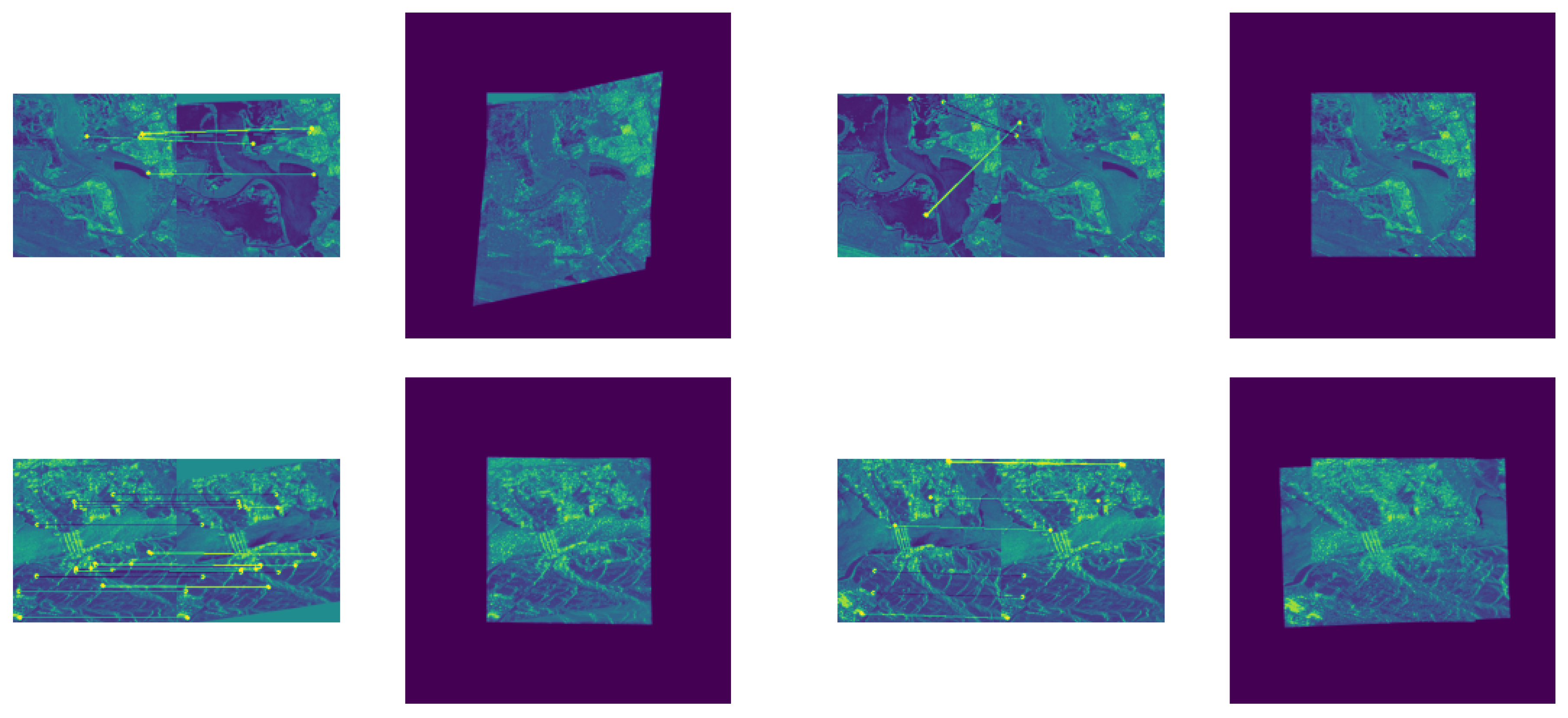
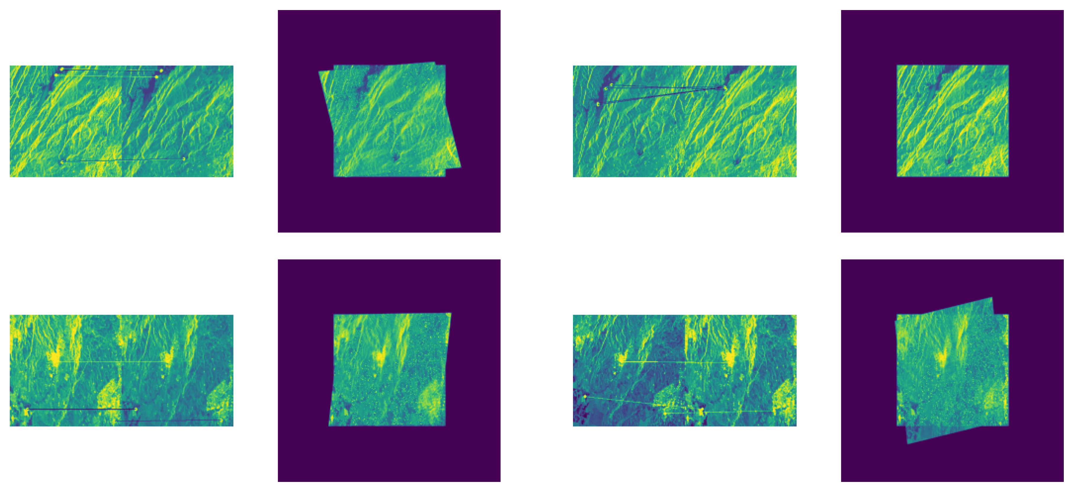
Figure 16, Figure 17 and Figure 18 demonstrate samples of matched feature point pairs obtained through re-registration and one-time registration of feature points extracted using SAR-SIFT for the three sets of test data samples. In comparison with the results from the previous set of experiments, it is evident that the feature point pairs acquired through SAR-SIFT are fewer than those obtained using SIFT.

In Figure 16, the connecting lines of the matching point pairs obtained from the once registration of sample 1 appear more cluttered, and all of them are incorrectly matched, resulting in a failed image registration. The outcome of the fusion processing displays only the sensed image. The fusion process merely presents the information from one of the images. Conversely, the corresponding matching point pairs acquired through re-registration align with the correct positions. The fusion image exhibits continuous splicing boundaries, a substantial overlap of most image regions, and the visibility of splicing boundaries between the two images. For sample 2, the positions of matched point pairs obtained from once-registration are accurate, resulting in successful image registration. However, the overlapping area of the fused image is blurred, which hinders the acquisition of image information. Re-registration, on the other hand, yields more correct matching point pairs, evenly distributed, with the fusion image displaying continuous splicing boundaries, extensive region overlap, and visible splicing boundaries and geometric structural features.

In Figure 17, feature point pairs derived from the once-registration of sample 1 are concentrated and inaccurately matched, and the image registration is failure. The fusion image primarily shows the sensed image. In contrast, feature point pairs acquired through re-registration for sample 1 correspond to the accurate location, with a relatively scattered distribution. The fusion image exhibits continuous splicing boundaries and substantial overlap in most image regions. For sample 2, both re-registration and once-registration yield accurately corresponding feature point pairs. The fusion images demonstrate extensive region overlap, with no noticeable misalignment in the splicing boundary.

The two samples in Figure 18 display evident linear structural features and grayscale similarity. In both cases, re-registration and once-registration yield correctly corresponding feature point pairs. The fusion images reveal significant overlap in most image regions, with continuous splicing boundaries, indicating a favorable registration outcome.

It’s crucial to note that in the context of SAR images, SIFT and SAR-SIFT can sometimes extract incorrect feature points or produce mismatched feature point pairs. As a result, the comparison between once-registration and re-registration, as presented above, serves as a reference. A comprehensive evaluation should encompass various indicators discussed in the preceding sections, along with other methodologies such as mosaicked images.

4.3.4. Data Visualization

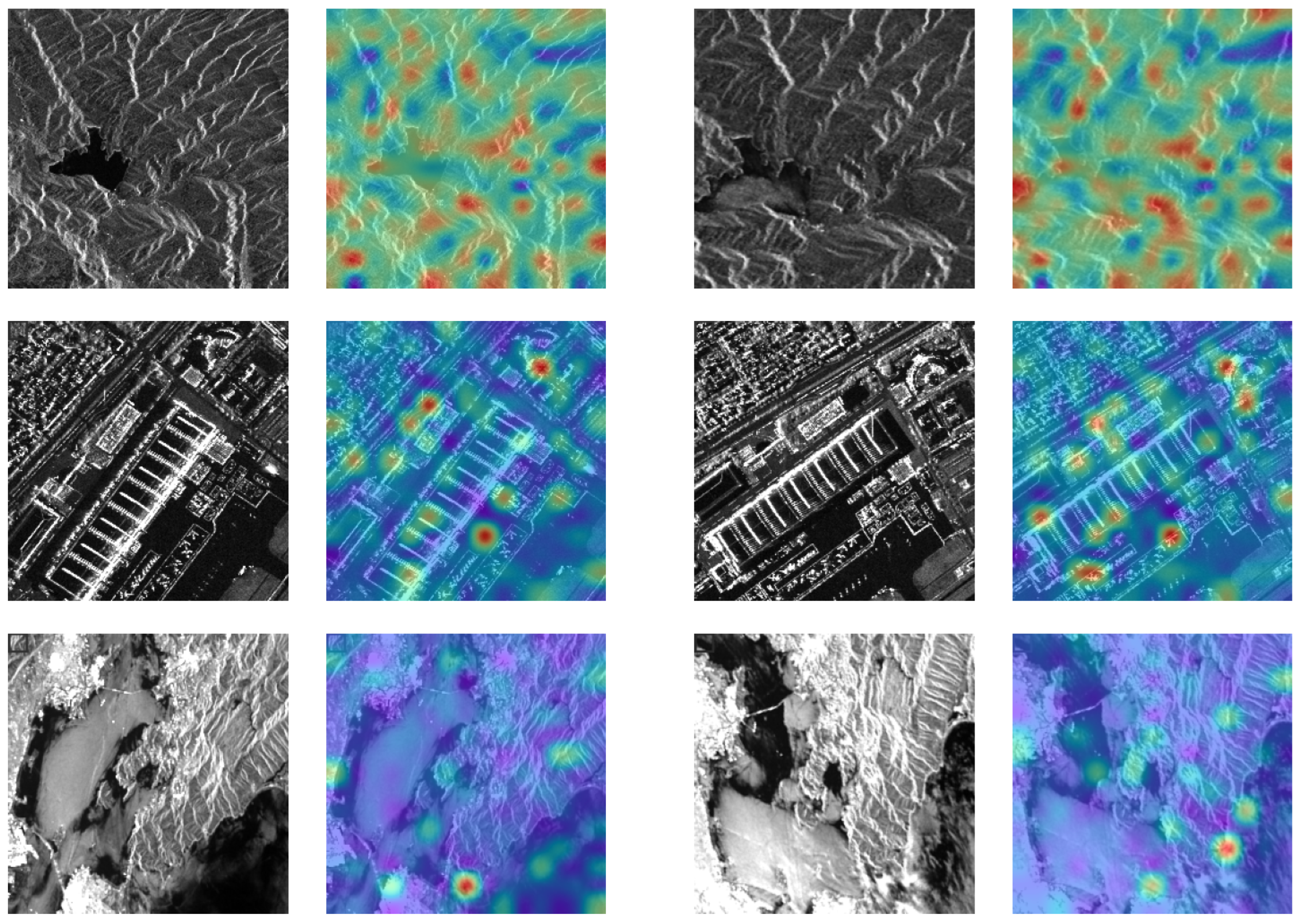
The visualization results of the test dataset samples are presented in Figure 19. These figures showcase the outcomes of attention maps, wherein each spatial location within the connectivity map encompasses all similarity scores between a feature in the reference image and all features within the sensed image. To illustrate, if a filter’s central patch comprises predominantly zeros except for a peak located at the top-left corner, the filter responds positively to features within the reference image that correspond to the top-left corner of the sensed image. Likewise, when numerous spatial locations of a filter yield similar visual responses, the filter demonstrates heightened sensitivity to spatially co-located features within the reference image that align with the corresponding positions in the sensed image.

The figures exhibit several attention maps that validate the presumption that the layer has acquired the ability to replicate local neighborhood consensus. This is evident as certain filters exhibit strong responsiveness to spatially co-located features within the reference image that match consistent spatial positions in the sensed image.

4.3.5. Analysis of Failed Cases

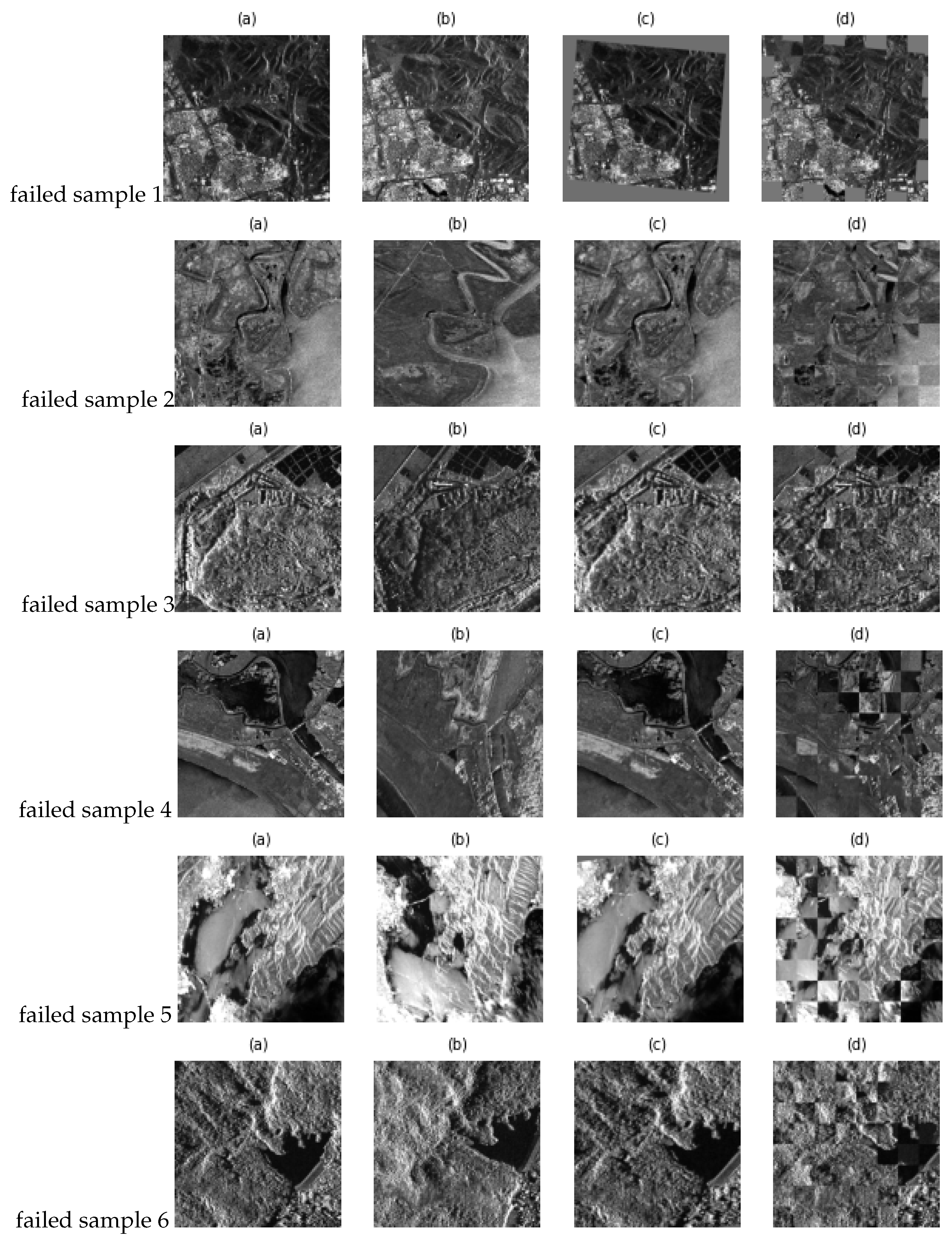
Figure 20 illustrates instances of failed registration. In the third column, the sensed image generated by the reinforcement learning framework of this paper is based on the reference image, i.e., the sensed image to be registered. The fourth column displays the outcomes of the registration using the method proposed in this paper. Variations in terrain features and imaging viewpoints between the sensed images obtained at different sampling times and the reference image pairs can lead to significant grayscale differences, as observed in failed sample 4, and different structural features, such as failed sample 3 and failed sample 6. In some cases, SAR images obtained from the same ground scene region may not appear intuitively identical, as demonstrated in rows 2 and 4 of the figure. While the reinforcement learning in this paper generates sensed images that partially reduce structural differences between them and the original reference images, it does not perform grayscale transformations on the sensed images.

The mosaic image of the sensed image and the reference image after the registration can exhibit pronounced grayscale misregistration at the splicing location, as seen in failed sample 5, or show insufficient smoothness in the splicing of line features and region features, as seen in failed sample 4. The registration scheme based on the entire image requires a certain level of grayscale and structural similarity between the sensed image and the reference image pairs to be registered. However, the reinforcement learning approach in this paper does not perform grayscale transformations on the SAR image during the transformation of the sensed image. Consequently, its applicability and scalability for registering SAR image pairs with substantial grayscale differences need to be enhanced.

Since this paper employs a self-learning method to generate training samples by applying various affine transformations to the training data, the feature differences between the sensed image and the reference image pairs that cannot be reflected by the affine transformations include significant geometric distortions, e.g., failed sample 3 and failed sample 6, and grayscale changes, e.g., failed sample 4. Such differences impact the correlation between image pairs, potentially leading to suboptimal performance of the registration method based on the correlation matching network presented in this paper. To address this challenge, a potential solution involves manually labeled matching labels and a machine learning network that performs grayscale transformations, image matching, and evaluation.

Furthermore, failed sample 1 highlights the significant challenge of dealing with complex and variable ground topographic features. In this scenario, the feature point pairs obtained by SAR-RL are sparse and unevenly distributed in the images to be registered, affecting the global registration performance of the image pairs. Some of the failure cases involve images with densely distributed point features and line features. This can be attributed to the fact that the SAR-RL in this paper is a global registration method, and the uniform distribution of weights for the globally densely distributed point features and line features can easily result in the failure of the registration.

5. Discussion

Registering SAR images of terrain undulating regions acquired under different imaging geometries presents a significant challenge due to inherent noise and geometric distortion in SAR images. The SAR-RL method presented in this paper adopts a global registration approach, but there are instances where registering SAR images of complex terrain regions encounters difficulties, particularly when the training dataset is generated through a self-learning scheme.

Future research endeavors will be directed towards enhancing the SAR-RL method. This will involve incorporating a priori knowledge of dataset distribution and optimizing training datasets by introducing diverse distribution patterns and supervision information. These efforts aim to enhance the accuracy and efficiency of the method across various datasets. Simultaneously, there is a consideration for adapting and deploying the trained neural networks to portable devices using TensorFlow Lite. Such an advancement would enable real-time applications by researchers and potentially even non-specialists.

Author Contributions

Conceptualization, Rong Zhou; methodology, Rong Zhou; software, Rong Zhou; validation, Rong Zhou; formal analysis, Rong Zhou; investigation, Rong Zhou and Gengke Wang; resources, Rong Zhou and Gengke Wang; data curation, Rong Zhou and Gengke Wang; writing—original draft preparation, Rong Zhou and Gengke Wang; writing—review and editing, Rong Zhou, Zhisheng Zhang. and Huaping Xu; visualization, Rong Zhou; supervision, Zhisheng Zhang; project administration, Rong Zhou; funding acquisition, Huaping Xu. All authors have read and agreed to the published version of the manuscript.

Funding

This research was funded by the National Natural Science Foundation of China grant number U2241202.

Data Availability Statement

Restrictions apply to the availability of the TerraSAR-X satellite images of the Zhuhai region in southern China, because datasets were purchased from [third party] by Professor Ze Yu from Beihang University. The source of other image data is contained within the article.

Acknowledgments

Thanks to Professor Jie Chen from Beihang University for providing a high-performance computer to product the training and test datasets. Thanks to Professor Ze Yu from Beihang University for providing TerraSAR-X satellite images of the Zhuhai region in southern China.

Conflicts of Interest

The authors declare no conflict of interest. The funders had no role in the design of the study; in the collection, analyses, or interpretation of data; in the writing of the manuscript; or in the decision to publish the results.

References

Gonçalves, H.; Gonçalves, J.A.; Corte-Real, L. Measures for an objective evaluation of the geometric correction process quality. IEEE Geoscience and Remote Sensing Letters 2009, 6, 292–296. [Google Scholar] [CrossRef]
Wang, S.; Quan, D.; Liang, X.; Ning, M.; Guo, Y.; Jiao, L. A deep learning framework for remote sensing image registration. ISPRS Journal of Photogrammetry and Remote Sensing 2018, 145, 148–164. [Google Scholar] [CrossRef]
Mao, S.; Yang, J.; Gou, S.; Jiao, L.; Xiong, T.; Xiong, L. Multi-Scale Fused SAR Image Registration Based on Deep Forest. Remote Sensing 2021, 13, 2227. [Google Scholar] [CrossRef]
Jaderberg, M.; Simonyan, K.; Zisserman, A.; others. Spatial transformer networks. Advances in neural information processing systems 2015, 28. [Google Scholar]
Schwegmann, C.P.; Kleynhans, W.; Salmon, B. The development of deep learning in synthetic aperture radar imagery. 2017 International Workshop on Remote Sensing with Intelligent Processing (RSIP). IEEE, 2017, pp. 1–2. [CrossRef]
Jianxu, M. Research on Three-Dimensional Imaging Processing Techniques for Synthetic Aperture Radar Interferometry (InSAR). PhD thesis, Hunan University, 2002.
Jie, R. Key Technology Research for Cartographic Applications of Multi-source Remote Sensing Data. PhD thesis, University of Chinese Academy of Sciences (Institute of Remote Sensing and Digital Earth, Chinese Academy of Sciences), 2017.
Yide, M.; Lian, L.; Yafu, W.; Ruolan, D. The Principles and Applications of Pulse-Coupled Neural Networks, 2006.
Del Frate, F.; Licciardi, G.; Pacifici, F.; Pratola, C.; Solimini, D. Pulse Coupled Neural Network for automatic features extraction from COSMO-Skymed and TerraSAR-X imagery. 2009 IEEE International Geoscience and Remote Sensing Symposium. IEEE, 2009, Vol. 3, pp. III–384. [CrossRef]
Zhao, C. SAR Image Registration Method based on SAR-SIFT and Deep Learning. Master’s thesis, Xidian University, 2017.
Hu, J.; Lu, J.; Tan, Y.P. Sharable and individual multi-view metric learning. IEEE transactions on pattern analysis and machine intelligence 2017, 40, 2281–2288. [Google Scholar] [CrossRef] [PubMed]
Fan, Y.; Wang, F.; Wang, H. A Transformer-Based Coarse-to-Fine Wide-Swath SAR Image Registration Method under Weak Texture Conditions. Remote Sensing 2022, 14, 1175. [Google Scholar] [CrossRef]
Quan, D.; Wang, S.; Gu, Y.; Lei, R.; Yang, B.; Wei, S.; Hou, B.; Jiao, L. Deep feature correlation learning for multi-modal remote sensing image registration. IEEE Transactions on Geoscience and Remote Sensing 2022, 60, 1–16. [Google Scholar] [CrossRef]
Li, L.; Han, L.; Ye, Y. Self-supervised keypoint detection and cross-fusion matching networks for multimodal remote sensing image registration. Remote Sensing 2022, 14, 3599. [Google Scholar] [CrossRef]
Blundell, C.; Uria, B.; Pritzel, A.; Li, Y.; Ruderman, A.; Leibo, J.Z.; Rae, J.; Wierstra, D.; Hassabis, D. Model-free episodic control. arXiv preprint arXiv:1606.04460 2016. [Google Scholar] [CrossRef]
Pritzel, A.; Uria, B.; Srinivasan, S.; Badia, A.P.; Vinyals, O.; Hassabis, D.; Wierstra, D.; Blundell, C. Neural episodic control. International Conference on Machine Learning. PMLR, 2017, pp. 2827–2836.
Savinov, N.; Raichuk, A.; Marinier, R.; Vincent, D.; Pollefeys, M.; Lillicrap, T.; Gelly, S. Episodic curiosity through reachability. arXiv preprint arXiv:1810.02274 2018. [Google Scholar] [CrossRef]
Lin, Z.; Zhao, T.; Yang, G.; Zhang, L. Episodic memory deep q-networks. arXiv preprint arXiv:1805.07603 2018. [Google Scholar] [CrossRef]
Hu, H.; Ye, J.; Zhu, G.; Ren, Z.; Zhang, C. Generalizable episodic memory for deep reinforcement learning. arXiv preprint arXiv:2103.06469 2021. [Google Scholar] [CrossRef]
Rocco, I.; Arandjelovic, R.; Sivic, J. Convolutional neural network architecture for geometric matching. Proceedings of the IEEE conference on computer vision and pattern recognition, 2017, pp. 6148–6157. [CrossRef]
Rong, Z.; Yuan, W.; Zhisheng, Z. Hierarchical Episodic Control. 2023. [Google Scholar] [CrossRef]
He, H.; Chen, M.; Chen, T.; Li, D. Matching of remote sensing images with complex background variations via Siamese convolutional neural network. Remote Sensing 2018, 10, 355. [Google Scholar] [CrossRef]

1	The original images were downloaded from: https://download.geoservice.dlr.de/supersites/files/

Figure 1. Image registration based on reinforcement learning.

Figure 2. Agent Network Structure.

Figure 3. Architecture of the correlation layer.

Figure 4. Self-learning.

Figure 5. Quick-look of the descending orbit right-looking SAR images acquired by TerraSAR-X satellite’s at diffrent periods in the Napa region, USA.

Figure 8. Options and Actions in testing process.

Figure 9. The checkerboard mosaicked image examples of registered images from test datasets.

Figure 10. Statistical analysis of RMSE values for 110 pairs of TerraSAR-X Napa 2014 images using SAR-SIFT.

Figure 11. Statistical analysis of RMSE values for 18 pairs of Sentinel-1A Napa 2014 images using SAR-SIFT.

Figure 12. Statistical analysis of RMSE values for 62 pairs of TerraSAR-X Zhuhai 2016 images using SAR-SIFT.

Figure 13. Examples of matching results based SIFT by re-registration and once-registration in TerraSAR-X Napa 2014 Dataset

Figure 14. Examples of matching results based SIFT by re-registration and once-registration in Sentinel-1A Napa 2014 Dataset

Figure 15. Examples of matching results based SIFT by re-registration and once-registration in TerraSAR-X Zhuhai 2016

Figure 16. Examples of matching results based SAR-SIFT by re-registration and once-registration in TerraSAR-X Napa 2014 Dataset

Figure 17. Examples of matching results based SAR-SIFT by re-registration and once-registration in Sentinel-1A Napa 2014 Dataset

Figure 18. Examples of matching results based SAR-SIFT by re-registration and once-registration in TerraSAR-X Zhuhai 2016

Figure 19. Visualization results of dataset test samples

Figure 20. failed registration samples

Table 1. Relationship between Normalized Root Mean Square Error and Options.

	$[0, 0.2)$	$[0.2, 0.4)$	$[0.4, 0.6)$	$[0.6, 0.8)$	$[0.8, 1)$	[1, )
TerraSAR-X Napa 2014	Option 0	Option 0	Option 0	-	Option 1	Option 1
Sentinel-1A Napa 2014	Option 0	-	-	-	Option 0	Option 1
TerraSAR-X Zhuhai 2016	Option 0	Option 0	-	Option 1	Option 1	Option 1

Table 2. Quantitative analysis of median results of metrics for re-registration , SAR-SIFT and DL-WangS.

TerraSAR-X Napa 2014 dataset
	$N_{r e d}$	$R M S E_{a l l}$	$R M S E_{L o o}$	$P_{q u a r d}$	$B P P (1.0)$	$S_{k e w}$	$S_{c a t}$	running time
SAR-SIFT	12	$0.7170$	$0.9021$	$0.0000$	$0.5000$	$0.4843$	$1.0000$	$28.4611$ s
DL-WangS	22	$0.3290$	$0.3977$	$0.0000$	$0.0498$	$0.3012$	$1.0000$	$9.5026$ s
Re-registration	7	$0.3257$	$0.4331$	$0.0000$	$0.0317$	$0.2943$	$0.9999$	-
Sentinel-1A Napa 2014 dataset
	$N_{r e d}$	$R M S E_{a l l}$	$R M S E_{L o o}$	$P_{q u a r d}$	$B P P (1.0)$	$S_{k e w}$	$S_{c a t}$	running time
SAR-SIFT	6	$0.8263$	$1.0324$	$0.6340$	$0.5000$	$0.0143$	$1.0000$	$17.3443$ s
DL-WangS	20	$0.3310$	$0.3449$	$0.1182$	$0.0023$	$0.1293$	$1.0000$	$9.2473$ s
Re-registration	4	$0.3714$	$0.4064$	$0.0931$	$0.0317$	$0.1169$	$0.9999$	-
TerraSAR-X Zhuhai 2016 dataset
	$N_{r e d}$	$R M S E_{a l l}$	$R M S E_{L o o}$	$P_{q u a r d}$	$B P P (1.0)$	$S_{k e w}$	$S_{c a t}$	running time
SAR-SIFT	23	$0.7669$	$0.8945$	$0.4045$	$0.7011$	$0.2349$	$0.9000$	$32.8332$ s
DL-WangS	30	$0.3591$	$0.4156$	$0.2812$	$0.0101$	$0.1058$	$0.9999$	$10.2314$ s
Re-registration	26	$0.3402$	$0.4911$	$0.1298$	$0.0061$	$0.011$	$1.0000$	-

Table 3. Quantitative analysis of mean results of metrics for re-registration , SAR-SIFT and DL-WangS.

TerraSAR-X Napa 2014 dataset
	$N_{r e d}$	$R M S E_{a l l}$	$R M S E_{L o o}$	$P_{q u a r d}$	$B P P (1.0)$	$S_{k e w}$	$S_{c a t}$	running time
SAR-SIFT	13	$0.8007$	$0.9451$	$0.0001$	$0.4201$	$0.3801$	$0.9997$	$32.1185$ s
DL-WangS	20	$0.2912$	$0.3071$	$0.0000$	$0.0032$	$0.2189$	$0.9999$	$9.8215$ s
Re-registration	10	$0.3092$	$0.3471$	$0.0000$	$0.0712$	$0.1324$	$0.9995$	-
Sentinel-1A Napa 2014 dataset
	$N_{r e d}$	$R M S E_{a l l}$	$R M S E_{L o o}$	$P_{q u a r d}$	$B P P (1.0)$	$S_{k e w}$	$S_{c a t}$	running time
SAR-SIFT	6	$0.8019$	$0.9733$	$0.5215$	$0.5991$	$0.1021$	$0.9999$	$22.4352$ s
DL-WangS	18	$0.2431$	$0.3130$	$0.1572$	$0.0169$	$0.0035$	$0.9999$	$9.0089$ s
Re-registration	6	$0.3119$	$0.4204$	$0.1874$	$0.0245$	$0.0097$	$0.9999$	-
TerraSAR-X Zhuhai 2016 dataset
	$N_{r e d}$	$R M S E_{a l l}$	$R M S E_{L o o}$	$P_{q u a r d}$	$B P P (1.0)$	$S_{k e w}$	$S_{c a t}$	running time
SAR-SIFT	20	$0.7395$	$0.862$	$0.4121$	$0.2422$	$0.2911$	$0.9333$	$30.9462$ s
DL-WangS	30	$0.3292$	$0.2213$	$0.3119$	$0.0102$	$0.051$	$1.0000$	$10.1931$ s
Re-registration	25	$0.3371$	$0.24324$	$0.2454$	$0.0014$	$0.068$	$1.0000$	-

Disclaimer/Publisher’s Note: The statements, opinions and data contained in all publications are solely those of the individual author(s) and contributor(s) and not of MDPI and/or the editor(s). MDPI and/or the editor(s) disclaim responsibility for any injury to people or property resulting from any ideas, methods, instructions or products referred to in the content.

© 2023 by the authors. Licensee MDPI, Basel, Switzerland. This article is an open access article distributed under the terms and conditions of the Creative Commons Attribution (CC BY) license (http://creativecommons.org/licenses/by/4.0/).

Copyright: This open access article is published under a Creative Commons CC BY 4.0 license, which permit the free download, distribution, and reuse, provided that the author and preprint are cited in any reuse.

MDPI Initiatives

Important Links

Choose an area of interest and we will send you notifications of new preprints at your preferred frequency.

Disclaimer

A Sub-second Method for SAR Image Registration Based on Hierarchical Episodic Control

Abstract

1. Introduction

2. Related Work

2.1. Deep Learning

2.2. Reinforcement Learning

3. Deep Reinforcement Learning-Based SAR Image Registration

3.1. SAR-RL

3.2. Model

3.2.1. Transformer

3.2.2. Correlation Layer

3.3. Option Episodic Memory

3.4. Self-Learning

4. Experiments

4.1. Dataset

4.2. Option Analysis

4.3. SAR Image Registration Results Analysis

4.3.1. Once-Registration and Re-registration

4.3.2. Qualitative Evaluation Results

4.3.3. Quantitative Evaluation Results

4.3.4. Data Visualization

4.3.5. Analysis of Failed Cases

5. Discussion

Author Contributions

Funding

Data Availability Statement

Acknowledgments

Conflicts of Interest

References

MDPI Initiatives

Important Links

Subscribe