Study of Nanoparticles by Dynamic Light Scattering: Processing Challenges

Vadim Annenkov

doi:10.20944/preprints202308.1929.v1

Submitted:

28 August 2023

Posted:

29 August 2023

You are already at the latest version

Abstract

Nanoparticles are of great importance for various scientific and technological applications, drug discovery, ecology, molecular biology, etc. Size is a basic characteristic of any particle, and dynamic light scattering is beyond competition when measuring particle size in dispersions ranging from nanometers to micrometers. Unfortunately, this method has a serious problem in processing and interpreting experimental data. Instrument noise and polydispersity of the sample lead to the situation when one initial autocorrelation function corresponds to several different particle size distributions. Sometimes these different solutions of the inverse task can be found by changing parameters in the software. Sometimes the scientist cannot be suspicious of possible other solutions, having one result from the program. In this article I demonstrate the problem on model and experimental data using three known programs: CONTIN, the Malvern Zetasizer and DynaLS. I also present my own free program Autocor, which allows to test our own hypotheses about the modality and shape of the particle size distribution by optimizing the parameters of our own models with a small number of degrees of freedom.

Keywords:

dynamic light scattering

;

autocorrelation function

;

inverse task

;

particle size distribution

Subject:

Chemistry and Materials Science - Polymers and Plastics

1. Introduction

Nanoparticles are widely present in almost every aspect of our lives. Individual macromolecules, macromolecular and supramolecular associates, including biomolecules, are nanoparticles. Inorganic clusters, such as aluminum-based compounds, are important in the design of antiperspirants and cements [1,2]. Viruses 100-200 nm in size are typical nanoparticles. Size is an important characteristic of nanoparticles and dynamic light scattering (DLS) is the "workhorse" of chemists, biologists and other specialists working with polymer solutions or nanoparticle dispersions. Unfortunately, progress in hardware development cannot solve the problems of interpreting the data obtained. The DLS method (see some details in Appendix A) begins with obtaining an autocorrelation function (g₁(q,t), ACF):

g_{1} (q, t) = \sum_{i = 1}^{n} I_{i} e x p (- t / τ_{i})

(1)

where q is magnitude of the scattering vector, t is the delay time, τ_i and I_i are the relaxation time and scattering intensity for a particle correspondingly.

The analysis of the experimental DLS data consists in finding the set of values I_i - τ_i that allows reconstructing the experimental ACF with the best statistical quality. Equation (1) is a special case of the Fredholm integral equation, which is the basis of many instrumental applications [3]. The main difficulty in solving such inverse tasks is that different solutions may give comparable fits to experimental data. A number of algorithms were developed in this area [4,5] (and references in this articles) and equipment manufacturers provide their own closed software. Nevertheless, the scientist is often left alone with the DLS instrument without a chance to compare different statistically similar solutions.

I have developed a free program, Autocor, in which the user can choose the model of particle size distribution (uniform, logarithmic Gaussian or Lorentz distribution) and the number of peaks. The program optimizes the peak position, intensity and dispersion similar to the Box centroid method [6], which gives a chance to find the global minimum of the sum of squares of residuals. This approach gives more power and responsibility to the scientist, who can test different models taking into account data from other methods and prior knowledge. In this article I compare Autocor and three known programs: CONTIN [4], Malvern Zetasizer software [7] and DynaLS that is distributed with the Photocor instrument [8].

2. Materials and Methods

I used the following programs:

2.1. CONTIN

CONTIN is the most well-known free software for processing DLS and other data [4,9]. This program was developed more than fifty years ago but it is still a powerful tool applied with such instruments as Bl-200SM Research Goniometer System from Brookhaven Instruments and Malvern Zetasizer (as payable additional software) [10,11]. The CONTIN program [4] was downloaded as FORTRAN file [12] and compiled with free Open Watcom compiler for Windows, Version 2.0 beta Nov 1 2017 21:42:29 (64-bit) [13]. Source and executable files, as well as the Microsoft Excel file for CONTIN results processing, are placed in the Data repository, folder "CONTIN".

2.2. Malvern Zetasizer Software

Malvern Zetasizer Software 7.11 has been applied to Malvern Zetasizer Nano-ZS data processing. This program does not allow the processing of arbitrary data, so it was not tested with model data. The free version of Malvern Zetasizer Software 7.11 was downloaded from the manufacturer's website [7].

2.3. DynaLS

The third program tested was DynaLS v2.8 (Alango Ltd., Israel). This program is part of the Photocor instrument software [8], but can be used by itself to process any ACF data.

2.4. Autocor

A free program Autocor have been developed by me. This program, unlike the three others, is based on the user's hypothesis about the number of peaks in the size distribution and the nature of these peaks (homogeneous, Gaussian or Lorentz distributions). The program optimizes the parameters of the model similar to the Box centroid method [6]. Briefly, a number of points (centroid) are created randomly in the definition area. Each point is characterized by peak position (relaxation time τ), peak intensity, and dispersion (in Gaussian or Lorentz models). A grid of τ with logarithmic distribution in the interval τ, where some scattering intensity is probable, is taken. τ - I curve, the calculated ACF and sum of squares of residuals (optimized parameter) are calculated for each centroid point. The optimized parameter is calculated for all points. The center of the centroid is calculated without the worst point. The coordinates of the worst point are reflected from the center with coefficient α, and it is the new point instead of the worst. If the new point is not better than the previous one, the coefficient α decreases or the worst point changes to the best one. These procedures continue until the centroid is folded into a single point with the necessary accuracy. Peak positions (relaxation time τ), peak intensities and dispersion (in Gauss or Lorentz models) are optimized separately. Size of the τ grid and other optimization parameters are tunable. The program generates a report in CSV (comma-separated values) format including particle size distribution when the corresponding parameters (laser wavelength, temperature, viscosity and refractive index) are set.

The source files and the program description can be found in folder "Autocor" in the Data repository (https://data.mendeley.com/datasets/jdbggcc627/2).

The Autocor program is written on C language with CodeLite 17.0.0 shell [14] and was compiled with TDM-GCC-64 10.3.0 release C compiler [15]. The code was also tested on HPC-cluster «Akademik V.M. Matrosov» (https://hpc.icc.ru), operating system CentOS Linux x86_64, GNU C compiler. The program code is free and open under Creative Commons Attribution 4.0 International Public License [16]. Briefly, anyone may copy, distribute, and modify the material for non-commercial purposes only. Any publication using this software must reference this article, and any changes to the code must be clearly described

3.1. Processing of model data

Model particle size distribution curves were constructed using Gaussian (lognormal) distributions. Instrumental noise was added as a random additive to the ACF, which decays with increasing delay time, since instrumental noise is more likely to occur at short values of t. The size distribution data were converted to ACF, and the ACF data were processed using the tested programs. The relaxation time was obtained and transformed into particle size, which was compared with the initial particle size distribution. Calculated ACF curves were compared with initial ACFs and the sum of squares of residuals (s₀) was calculated:

s_{0} = \sqrt{(\sum_{i = 1}^{N} e_{i}^{2}) / (N - 2)},

(2)

where

e_{i} = g_{2 i} - {\hat{g}}_{2 i}

,

{\hat{g}}_{2 i}

is calculated ACF value and N – number of points in ACF.

In the case of a model or experimental ACF containing some random noise, the autocorrelation coefficient was calculated as:

ρ = |\frac{\sum_{i = 2}^{n} e_{i} \times e_{i - 1}}{\sum_{i = 1}^{n} e_{i}^{2}} \times \frac{n}{n - 1}|,

(3)

where e_i is residual value for point i, n – number of ACF points [17]. Lower value of ρ is the evidence of a better quality of the model because of lower autocorrelation of the residuals.

3. Results and discussion

3.1. Processing of model data

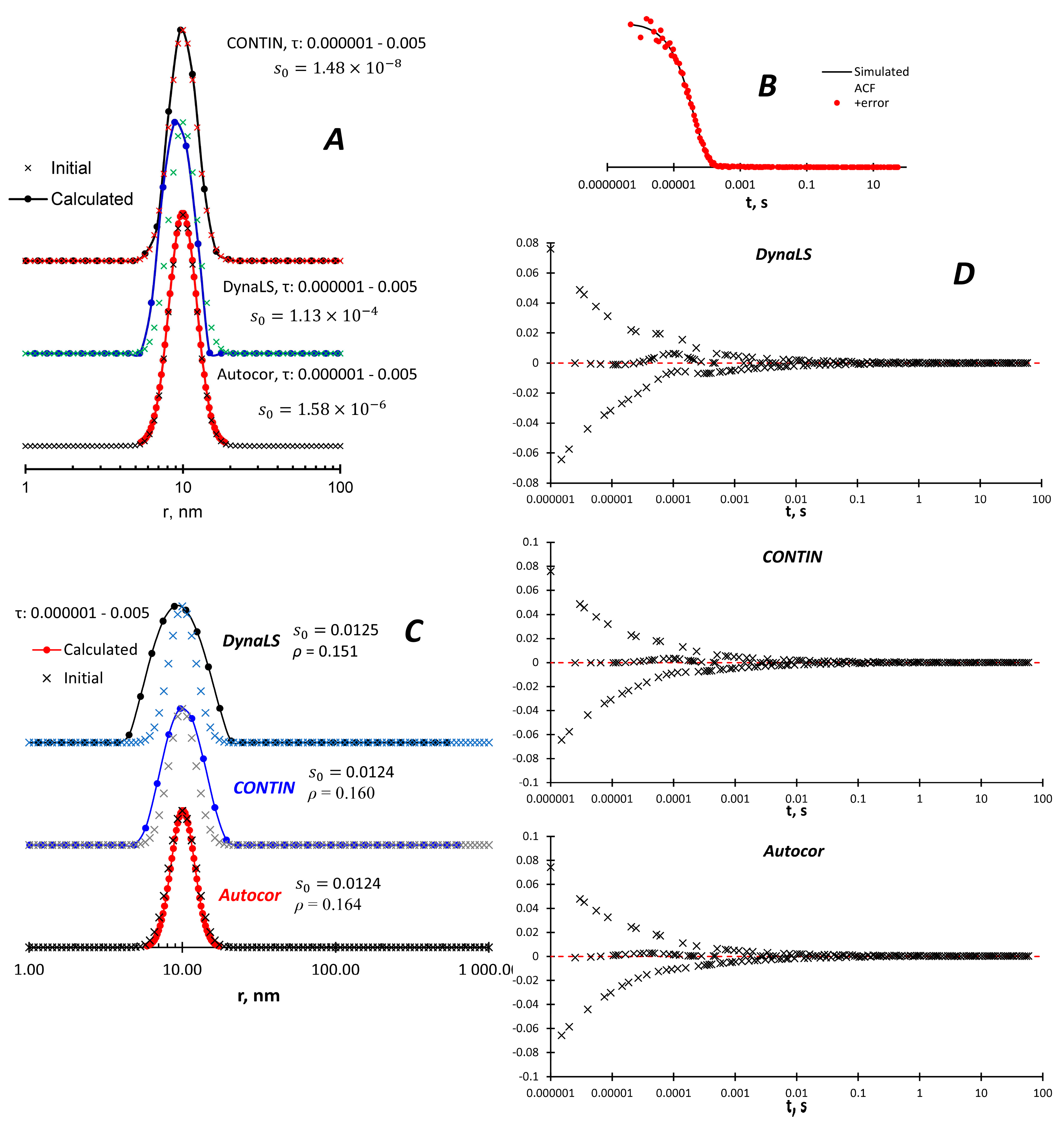
The simulated monomodal curves are adequately reproduced by all three methods (Figure 1A). In order to better simulate real data, random noise was added to the ACF, mostly at short delay times where hardware noise is more likely (Figure 1B). All methods found the same maximum size distribution (Figure 1C) with very close values of s₀ and ρ, as well as the residual distribution (Figure 1D). Autocor almost perfectly reproduces the original size distribution, CONTIN and especially DynaLS give broader peaks.

DLS gives the average radius of the particles, but often this method is used to answer the question: how many modes are in the size distribution? This information is needed to understand - can static light scattering (SLS) be used to measure the radius of gyration and molecular weight in the case of polymers? The intensity of scattered light increases in proportion to the radius to the sixth degree (for spherical particles) [18]. Thus, if we have two kinds of particles that differ significantly in radius, the SLS data will preferably reflect large particles which could be the minor fraction.

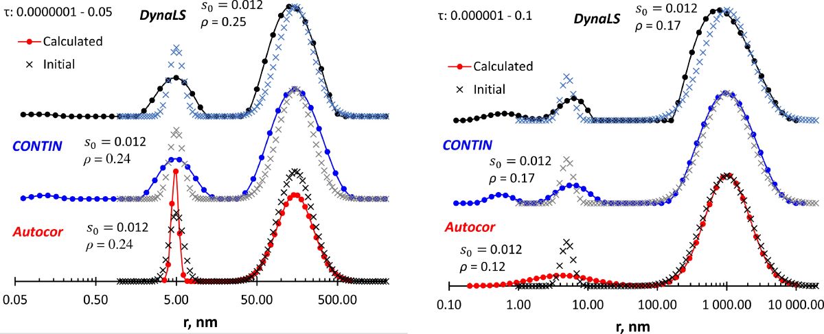
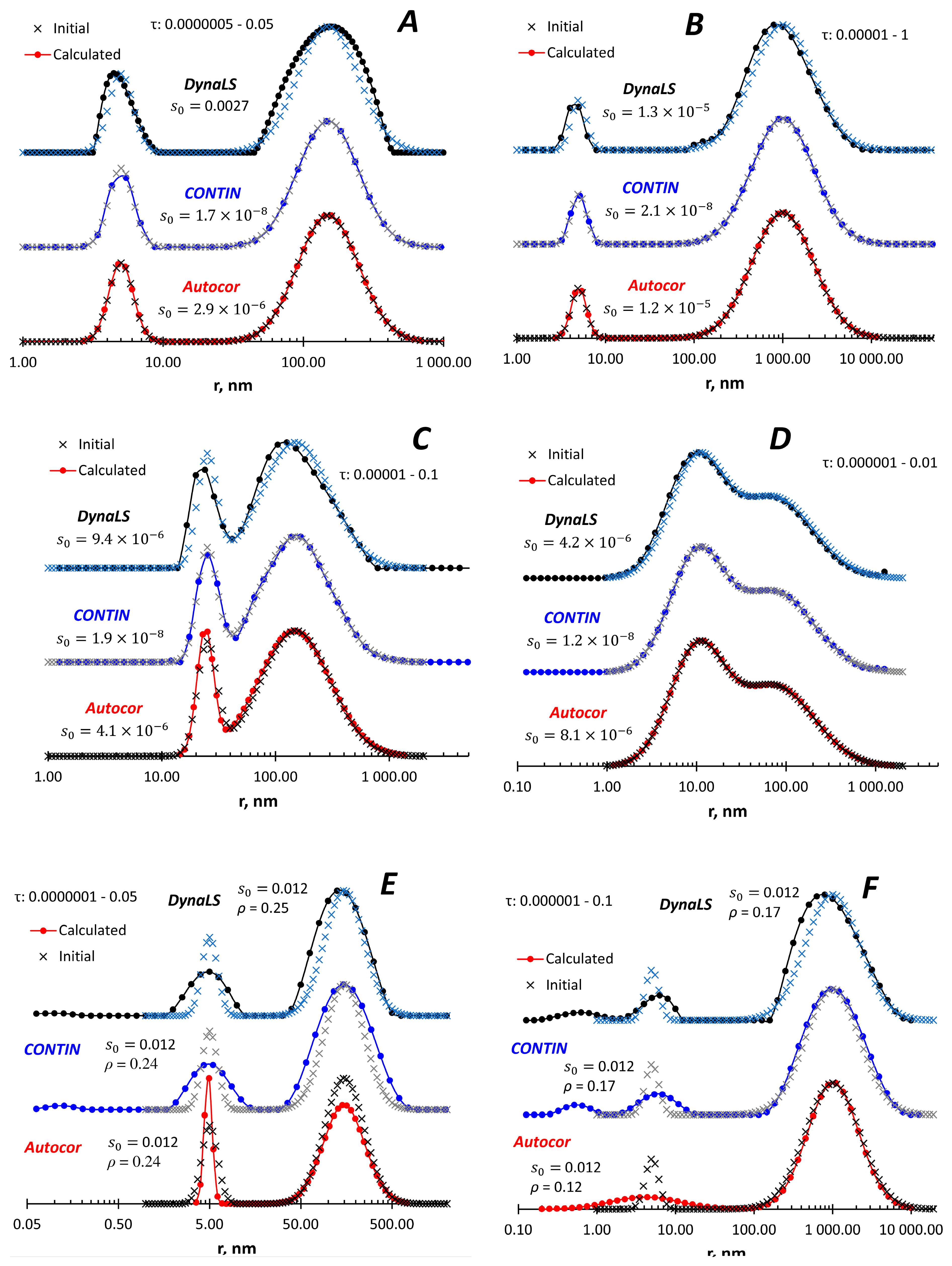
I have simulated four bimodal distributions, which differ in the distance between the peaks and the relative intensity of the peaks. Like the monomodal distribution, all three programs adequately reproduce the size distribution (Figure 2A-D). In the case of two isolated peaks after adding random noise to the ACF after adding random noise to the ACF (Figure 2E), all programs satisfactorily reproduced the original size distribution. When the peaks are more distant from each other and the low-size peak is less intense (Extended Data Figure 2F), all programs reproduce the large-size peak, but expand the low-size peak, especially Autocor. DynaLS and CONTIN show an artifact peak below 1 nm.

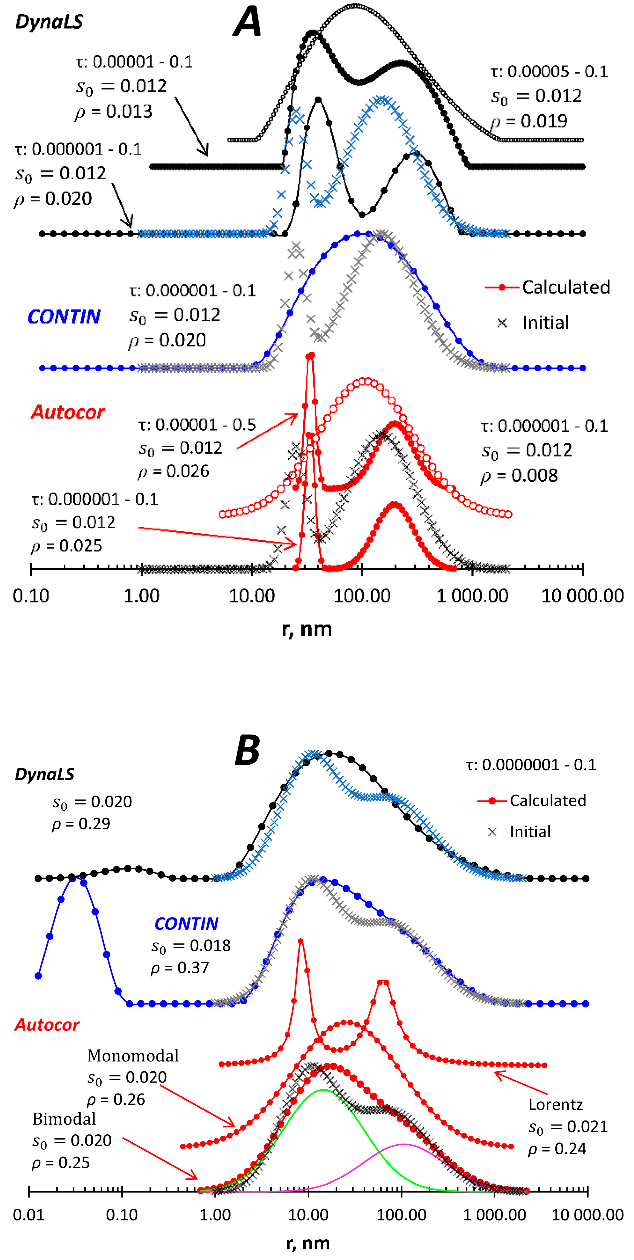
Figure 3 show closely located peaks. We see that CONTIN does not resolve the peaks in both cases, and changing the calculation parameters (τ interval, number of grid points) had no positive effect (data not shown). In the case of visible peaks (Figure 3a), DynaLS gives different results depending on the τ interval and shows one asymmetric peak when the initial size distribution looks like a peak with a shoulder (Figure 3b). The bimodal lognormal model in Autocor shows both peaks in Figure 3a regardless of the τ interval, but it should be noted that the monomodal lognormal model also satisfies the input data with a similar fitting result. Two peaks in Figure 3b can be detected with Autocor when the bimodal Lorentz model is applied. The lognormal model gives an asymmetric peak, which consists of two peaks easily obtained from the program output. And as in Figure 3a, the monomodal lognormal model also fits the input data.

3.2. Processing of experimental data

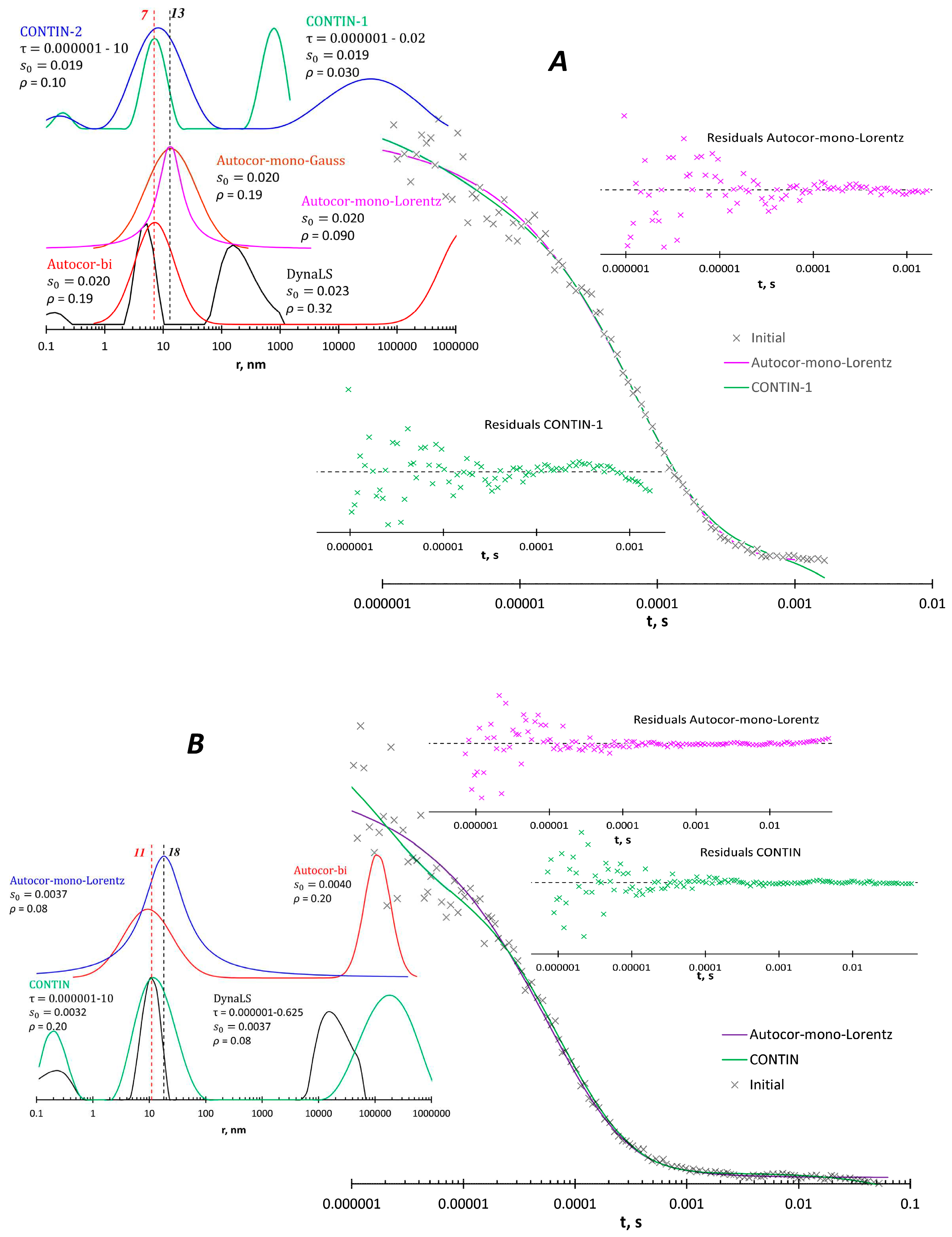
Water solution of poly(N-vinyl formamide) (PVFA) was studied with Photocor instrument (Figure 4). A 109 kDa fraction obtained according to [19] was used. PVFA is a hydrophilic non-ionizable polymer that has no reason to associate in an aqueous medium. Processing of the ACF with CONTIN and DynaLS software shows artifact peaks below 1 nm and peaks at 10 or more ηm, which are also difficult to attribute to any physical objects. These programs show peaks between 100 and 1000 nm at 90^o scattering angle. The Autocor software within the bimodal model shows peaks near 10 nm and above 10 ηm. Other programs also show a peak near 10 nm, so this particle size is reliable. What is interesting, Autocor in the monomodal Lorentz model gives a peak at 13-18 nm with statistical parameters comparable to the description of the size distribution by several peaks.

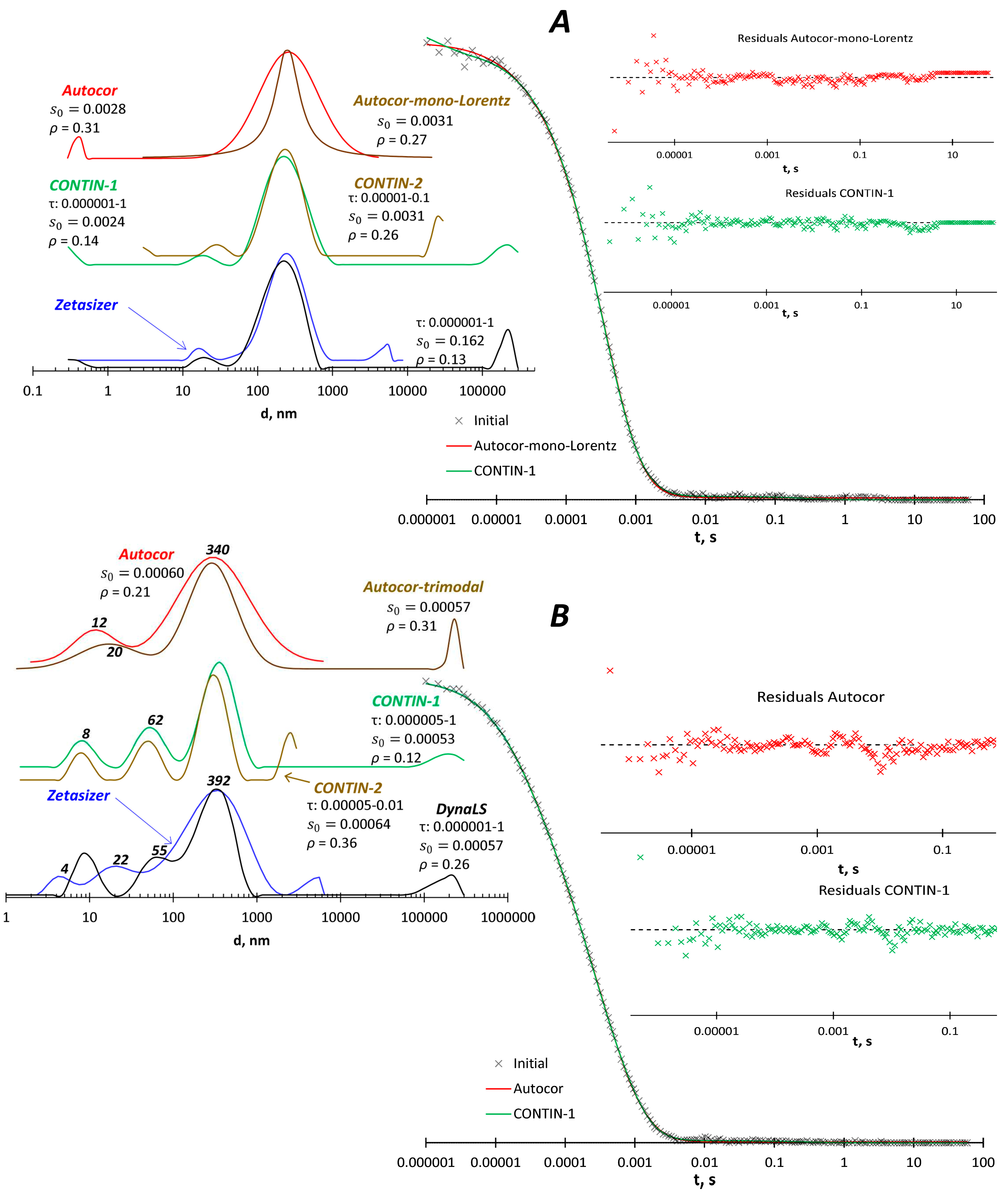
Malvern Zetasizer machine was applied to measure size of particles in aqueous solutions of two polymers: co(acrylic acid – vinylamine), sample PV20-13g from [20] and polymer P11 with grafted amine groups from [21]. In the case of PV20-13g copolymer (Figure 5A), the Zetasizer software shows a trimodal curve with peaks at 16, 250 and 550 nm. DynaLS and CONTIN give the same large peak at 250 nm and a small peak at 15-30 nm, as well as some artifacts below 1 nm and above 100 µm. The Autocor program in the bimodal model gives a peak at 250 nm and an artifact below 1 nm; moreover, the monomodal model with the Lorenz distribution shows a narrower peak at 250 nm with an adequate fitting, except for the region above 1 s, which is not informative for this sample. Thus, the presence of 15-30 nm particles in this solution is questionable and should be verified by further studies, e.g., at different pH and ionic strength values, which may reduce the ability of macromolecules to associate.

The Zetasizer software shows four peaks at 4, 22, 392and 5500 nm for P11 polymer (Figure 5B). DynaLS and CONTIN show peaks of 8, 55-62, 330-390 nm and artifact above 10-100 µm. The bimodal model in Autocor gives peaks of 12 and 340 nm, and the fit is close to the CONTIN results. The trimodal model in Autocor adds a peak above 100 µm and does not show particles in the 50-60 nm size.

5. Conclusions

Thus, the processing of simulated and experimental ACF using different programs confirms the presence of significantly different solutions for the same input data. Moreover, by changing the calculation parameters, such as the interval τ of the solution, we have different solutions for the same program. The situation becomes critical when we have to decide on the modality of the particle size distribution, for example, before experiments on static light scattering or when analyzing compositions for injections into the blood. The examples given in this article show that in some cases DLS data can be interpreted using relatively simple models with a small number of degrees of freedom (one or two lognormal or Lorentzian peaks). The Autocor program presented here is the tool that allows researchers to analyze DLS data with these simple models and optimize the model parameters with a high probability of finding a global optimum. This approach is an alternative to user-independent algorithms and can be useful when DLS data are ambiguous and other information (electron microscopy, SEC, etc.) is available.

Funding

This research was funded by the Russian Science Foundation, grant number 22-15-00268.

Data Availability Statement

The Autocor code, instructions and calculation data are available from the Digital Commons Data repository (https://data.mendeley.com/datasets/jdbggcc627/2).

Acknowledgments

The author wish to thank the Irkutsk Supercomputer Center of SB RAS for providing the access to HPC-cluster "Akademik V.M. Matrosov". I am extremely grateful to Dr. Vladimir Aseev, who introduced me to DLS and drew my attention to ambiguity of results obtained with DLS.

Conflicts of Interest

The funders had no role in the design of the study; in the collection, analyses, or interpretation of data; in the writing of the manuscript; or in the decision to publish the results.

Appendix A

A brief description of the DLS theory

The DLS method begins with obtaining an autocorrelation function (ACF) [22]:

g₂(q,t) = <i(0)i(t)>/<i(∞)>²,

(1)

where i is scattering intensity at various times: initial, i(0), at delay time

\to \infty

and at delay time t. Angle brackets < > denote the average value over many repetitions. q is magnitude of the scattering vector:

q = 4πn₀/λ∙sin(Θ/2),

(2)

where n₀ is the solvent refractive index, λ is the laser wavelength and Θ is the scattering angle.

The g₂ (or g₂ – 1) values are the raw data obtained from DLS experiments. DLS data processing deals with the function g₁(q,t) from the equation:

g₂(q,t) = 1 + β[g₁(q,t)]²,

(3)

where β is called "intercept", it is value of (g₂(q,t) -1) at t = 0. g₁(q,t) is connected with relaxation time τ:

g_{1} (q, t) = e x p (- t / τ),

(4)

and 1/τ = D_tq², where D_t is the translation diffusion coefficient which allows to calculate hydrodynamic radius (r_h) of the particle according to the Stokes-Einstein equation:

r_h = k_BT/(6πηD_t),

(5)

where k_B is the Boltzmann constant, T is temperature and η is viscosity of the solvent.

These equations allow us to find r_h in the case of monodisperse particles. Real systems consist of a mixture of different particles and g₁(q,t) is a sum of many functions:

g_{1} (q, t) = \sum_{i = 1}^{n} I_{i} e x p (- t / τ_{i})

(6)

where I_i is scattering intensity from the corresponding particles.

The analysis of the experimental DLS data consists in finding the set of values I_i - τ_i that allows reconstructing the experimental ACF with the best statistical quality. The particle sizes are obtained from the values of τ using equation (5).

References

Dawn, A.; Wireko, F.C.; Shauchuk, A.; Morgan, J.L.L.; Webber, J.T.; Jones, S.D.; Swaile, D.; Kumari, H. Structure–function correlations in the mechanism of action of key antiperspirant agents containing Al(III) and ZAG salts. ACS Appl. Mater. Interfaces 2022, 14, 11597–11609. [CrossRef]
Cerro-Prada, E.; Vázquez-Gallo, M.J.; Alonso-Trigueros, J.; Romera-Zarza, A.L. Nanoscale agent based modelling for nanostructure development of cement. In: Nanotechnology in Construction, 3; Bittnar, Z., Bartos, M.P.J., Němeček, J., Šmilauer, V., Zeman, J., Eds.; Springer: Berlin, Heidelberg, 2009; pp 175–180. [CrossRef]
Gear, C.W.; Vu, T. Smooth numerical solutions of ordinary differential equations. In: Numerical Treatment of Inverse Problems in Differential and Integral Equations. Progress in Scientific Computing, Deuflhard, P., Hairer, E., Eds.; Birkhäuser Boston, 1983; 2, pp. 2-12. [CrossRef]
Provencher, S.W. CONTIN: a general purpose constrained regularization program for inverting noisy linear algebraic and integral equations. Comput. Phys. Commun. 1982, 27, 229-242. [CrossRef]
Wang, Q.; Shen, J.; Thomas, J.C.; Wang, M.; Li, W.; Wang, Y Particle size distribution recovery from non-Gaussian intensity autocorrelation functions obtained from dynamic light scattering at ultra-low particle concentrations. Powder Technol. 2023, 413, 118033. [CrossRef]
Box, M.J. A new method of constrained optimization and a comparison with other method. Comput. J. 1965, 8, 42-52. [CrossRef]
Malvern Panalytical Ltd, Download page for the Zetasizer software. https://www.malvernpanalytical.com/en/support/product-support/zetasizer-range/zetasizer-nano-range/zetasizer-nano-zs#software, accessed: August, 2023.
LLC "Fotokor", Description of Dynals software. https://www.photocor.ru/products/dynals, accessed: August, 2023.
Provencher, S.W. A constrained regularization method for inverting data represented by linear algebraic or integral equations. Comput. Phys. Commun. 1982, 27, 213-227. [CrossRef]
Brookhaven Instruments, Description of BI-200SM Research Goniometer System. https://www.brookhaveninstruments.com/product/bi-200sm-research-goniometer/, accessed: August, 2023.
U. Nobbmann, Advanced research software features for the Zetasizer Nano. https://www.materials-talks.com/advanced-research-software-features-for-the-zetasizer-nano/, accessed: August, 2023.
S.W. Provencher, The CONTIN page. https://s-provencher.com/contin.shtml, accessed: August, 2023.
Open Watcom, Current-build. https://github.com/open-watcom/open-watcom-v2/releases/tag/Current-build, accessed: August, 2023.
CodeLite, An open source, free, cross platform IDE. https://codelite.org/, accessed: August, 2023.
Eubank, J.M. Tdm-gcc, GCC compiler. https://jmeubank.github.io/tdm-gcc/articles/2021-05/10.3.0-release, accessed: August, 2023.
Creative Commons, Attribution-NonCommercial 4.0 International lisence. https://creativecommons.org/licenses/by-nc/4.0/, accessed: August, 2023.
Borghers, E. & Wessa, P. Statistics - Econometrics – Forecasting. (Chicago Univ. Press, Office for Research Development and Education, 2004. https://www.xycoon.com/lsserialcorrelation.htm.
Chong, C.S.; Colbow, K. Light scattering and turbidity measurements on lipid vesicles. Biochim. Biophys Acta – Biomembr. 1976, 436, 260-282. [CrossRef]
Pavlov, G.M.; Korneeva, E.; Ebel, C.; Gavrilova, I.I.; Nesterova, N.A.; Panarin, E.F Hydrodynamic behavior, molecular mass, and conformational parameters of poly(vinylformamide) molecules. Polym. Sci. Ser. A 2004, 46, 1063-1067. https://www.elibrary.ru/item.asp?id=13464968. Text in Russian: https://elibrary.ru/download/elibrary_17370946_19152657.PDF.
Danilovtseva, E.N.; Palshin, V.A.; Strelova, M.S.; Lopatina, I.N.; Kaneva, E.V.; Zakharova, N.V.; Annenkov, V.V. Functional polymers for modeling the formation of biogenic calcium carbonate and the design of new materials. Polym. Adv. Technol. 2022, 33, 2984-3001. [CrossRef]
Danilovtseva, E.N.; Maheswari, K.U.; Pal'shin, V.A.; Annenkov V V. Polymeric amines and ampholytes derived from poly(acryloyl chloride): synthesis, influence on silicic acid condensation and interaction with nucleic acid. Polymers 2017, 9, 624. [CrossRef]
Burchard, W. Solution Properties of Branched Macromolecules. In: Branched Polymers II. Advances in Polymer Science, Roovers, J.; Ed.; Springe: Berlin, Heidelberg, 1999; V. 143 pp. 113-194. [CrossRef]

Figure 1. Simulated size distribution data and calculated curves for monomodal size distribution. A – initial data; B - simulated ACF after adding random noise; C - simulated and calculated curves after adding random noise to ACF curve; D - residuals after processing monomodal data with addition of noise. Calculation details and files are in folders "Mono_NoNoise" and "Mono_Noise" in the Data repository. τ (s) - values of the parameters used in the programs.

Figure 2. Simulated size distribution data and calculated curves for bimodal size distribution. A-D – initial data; E and F - simulated and calculated curves after adding random noise to ACF curve. Calculation details and files are in folders "Bi-XX NoNoise" and "Bi-XX Noise" in the Data repository. τ (s) - values of the parameters used in the programs.

Figure 3. Simulated size distribution data and calculated curves for bimodal size distribution after adding random noise to ACF curve. The initial peaks are at 25 and 150 nm (A) and 10 and 75 nm (B). Calculation details and files are in folders "Bi-3 Noise" and "Bi-4 Noise" in the Data repository. τ (s) - values of the parameters used in the programs.

Figure 4. Size distribution curves and fitting data for PVFA 1 g/L water solution at 20^oC. Laser wavelength 637 nm, scattering angles 90^o (A) and 120^o (B). Calculation details and files are in folder "Photocor" in the Data repository.

Figure 5. Size distribution curves and fitting data for co(acrylic acid – vinylamine) copolymer PV20-13g (A) and polymer P11 with grafted amine groups (B) in 1 g/L water solution at 20^oC. Laser wavelength 633 nm, scattering angle 173^o. Calculation details and files are in folder "Zetasizer" in the Data repository.

Disclaimer/Publisher’s Note: The statements, opinions and data contained in all publications are solely those of the individual author(s) and contributor(s) and not of MDPI and/or the editor(s). MDPI and/or the editor(s) disclaim responsibility for any injury to people or property resulting from any ideas, methods, instructions or products referred to in the content.

© 2023 by the authors. Licensee MDPI, Basel, Switzerland. This article is an open access article distributed under the terms and conditions of the Creative Commons Attribution (CC BY) license (http://creativecommons.org/licenses/by/4.0/).

Copyright: This open access article is published under a Creative Commons CC BY 4.0 license, which permit the free download, distribution, and reuse, provided that the author and preprint are cited in any reuse.

Study of Nanoparticles by Dynamic Light Scattering: Processing Challenges

Abstract

Keywords:

Subject:

1. Introduction

2. Materials and Methods

2.1. CONTIN

2.2. Malvern Zetasizer Software

2.3. DynaLS

2.4. Autocor

3.1. Processing of model data

3. Results and discussion

3.1. Processing of model data

3.2. Processing of experimental data

5. Conclusions

Funding

Data Availability Statement

Acknowledgments

Conflicts of Interest

Appendix A

A brief description of the DLS theory

References

MDPI Initiatives

Important Links

Subscribe