Preprint
Article

Ship Roll Prediction and Parameter Identification under Unknown Ocean Disturbances

Altmetrics

Downloads

137

Views

62

Comments

0

Submitted:

29 August 2023

Posted:

29 August 2023

You are already at the latest version

Alerts
Abstract
This paper investigates the roll parameter estimation of periodic disturbances where the amplitude, frequency, offset, and phase are hardly recognized in real practice. The key problem is to make an estimation that could eliminate the unknown disturbance parameters. An adaptive mechanism applies these four parameters to the globally exponential convergence using linear second-order filters and parameter estimation errors. Then, a backstepping controller is employed to make an exponential convergence to zero of the state variables. Moreover, reservoir computing is used to forecast chaotic roll motions to support predictability using Lyapunov exponents and the Poincaré map. Numerical simulations are demonstrated to validate the dynamical behaviors and efficacy of the proposed control scheme with machine learning.
Keywords: 
Subject: Engineering  -   Marine Engineering

1. Introduction

Estimating the sinusoidal signal is a significant problem for the control system. It is essential to identify the parameters of unknown periodical excitations in tracking and rejection control [1-2]. For example, estimating the frequencies of unknown disturbances in practice is difficult because the waves acting on a ship are nonstationary and unknown in advance [1]. Under maneuvering conditions, it could hardly measure the exact amounts of time-varying disturbances for a ship, such as waves, winds, currents, ice-covered waters, green waters, etc. To realize the safe voyage of a nonlinear vessel in unexpected sea situations, this paper investigates the parameter estimation of unknown disturbances and the suppression of chaotic roll motions with its prediction.
It is known that a periodic excitation consists of the sum of frequency, amplitude, bias (offset), and phase (randomness). The word periodic is still careful since it is close to approximately periodic, including perfect condition [3]. As for the real-time processing of chaotic motion in nonlinear systems, a potential solution based on Fourier analysis is deemed one of the unwelcome methods owing to the maximization of the periodogram [4]. Beyond the perspective of signal processing only, further study is needed to converge the parameter estimation related to the tracking performance of adaptive mechanisms [5]. The effect of nonlinear plants on parameter convergence is well explained in [6].
A similar work [4] identified the full parameters using a fifth-order estimator, showing the complexity and computational cost. The frequency and other parameter estimation techniques are separated in the present paper. Other parameter estimations of amplitude, bias, and phase are treated using the simple update law without any observers, as in [2, 7]. To design the disturbance rejection control, precise frequency estimation will be guaranteed with finite-time convergence like [1]. As for the problem of periodic disturbance cancellation, readers may refer to [8].
To achieve the stability and robustness of a nonlinear system [5], this paper implements linear second-order filters and parameter estimation errors to converge the global parameter estimation without a higher-order estimator. Such a filter operation [9] overcomes the infinitely increasing auxiliary vector [10]. Then, a backstepping control will be designed to suppress the chaotic roll motions of the nonlinear system under regular disturbances.
Chaos is aperiodic, long-term motion in a deterministic system [11]. Even slight initial conditions (IC) changes result in various outcomes [12]. From a positive viewpoint, the sensitiveness of a chaotic dynamical system has merit because, without the whole reconstruction of a system, it shows a different periodic orbit using a light adjustment of parameters [13]. However, controlling the nonperiodic behaviors of a chaotic system is not a trivial issue in the real world.
Recently, a simple or complex system under a veil of chaos has been studied with machine learning (ML) techniques, which contribute to predicting dynamic behaviors [14]. Notably, echo state networks (ESN, [15]), which are termed reservoir computing (RC, [16]), are efficient and easy to apply to black box modeling of dynamical systems [17]. As it is known, RC is a recurrent neural network (RNN)-based framework [18] that enables the readout to extract the desired output using a linear mapping [19]. The sensitivity of a chaotic system challenges long-term prediction [12], which only works if the initial uncertainty is not quickly multiplied by the evolution law [20]. However, RC is preferable for long-term prediction because it remembers past values and handles external disturbances, where all the past elements are implicitly contained in a state vector [18]. Moreover, this paper briefly starts to predict the chaotic roll motions before their manipulation and employs the Lyapunov exponents and the Poincaré map.
The remainder of the paper is organized as follows: A prediction scheme with RC, control synthesis for chaotic roll regulation using backstepping, estimation of frequency, and other parameters will be studied in Section 2. Some numerical simulations verify the proposed schemes in Section 3. The dynamical theory will be used to explore the uncontrolled chaotic roll responses using the bifurcation diagram, Poincaré map, and Lyapunov exponents (LEs). Finally, final remarks are given along with the following research directions in Section 4.

2. Materials and Methods

2.1. Prediction of chaotic roll motions using RC

One may experience walking around Lotus Pond, where the green leaves are naturally situated in a reservoir. In contrast to conventional RNN, only the readout weight is trained; input weight ( W i n ), feedback weight ( W f b ), and adjacency matrix ( W r e s ) are fixed and chosen randomly. In some simple applications where feedback response is not required, W f b can be omitted [21]. Based on similar effects on reservoirs, W i n , and W f b are primarily constructed similarly. Both input and feedback responses can be used for generating output [22]. For a reservoir with N neurons, the structure of a general ESN, having N reservoir states r N , I inputs u i n I , and O outputs y o u t O , is illustrated in Figure 1 [21]. The linear mapping input-output at a perceptron is presented in Figure 1.
According to [22, 23], the complete form of the update equation for reservoir state vector r(n) is defined as follows:
r ˜ ( n ) = tanh ( W i n [ b i n u i n ( n ) ] + W r e s r ( n ) + W f b y o u t ( n 1 ) )
r ( n ) = ( 1 α ) r ( n 1 ) + α r ˜ ( n )
where b i n is the bias of the reservoir’s input; u i n is the input fed to the reservoir at the sample n t h ; W i n is the input weight matrix from input to the reservoir; W r e s is the adjacency matrix describing the connection of the nodes in the reservoir; W f b is the feedback weight matrix from the output back to the reservoir, α is the leaking rate ( 0 α 1 ); f ( x ) = tanh ( x ) is the activation function. The weighted sum of the input states is then fed through an activation function to give the final output. The most basic activation function is the step function. However, smooth (sigmoid) functions are mostly preferred, such as hyperbolic tangent functions tanh ( x ) . Equations (1) and (2) indicate that the reservoir state r ( n ) will be updated based on the current input u i n and the feedback from the previous sample y o u t ( n 1 ) . The feedback term can be omitted in some tasks where the feedback state is unnecessary. The output state y o u t of the reservoir at the sample is achieved from a linear relationship of the reservoir state and input state as below [22,23]
y o u t ( n ) = W o u t r ( n )
where W o u t is the weight matrix from the reservoir to the output. In the training procedure, the input data is the reference data (teacher data). The actual output of the reservoir would be replaced by the desired output [22]. Within a training duration of T samples, all input and output data will be collected into matrices Y ( N y × T ) and X ( N x × T ) , by concatenating T columns Y ( n ) = y r e f ( n ) and r ( n ) = [ b o u t , u r e f ( n ) , r ( n ) ] T . Regarding equation (3), the linear relation between Y and X is defined as
Y = W o u t X
At the end of the training phase, the trained weight matrix W o u t can be computed analytically using Ridge regression.
W o u t = Y X T ( X X T + ν I ) 1
where ν is a parameter added to avoid overfitting. After the training phase, the output weight W o u t is computed and can be used for continuous computation. The actual output of the iteration can be reapplied as input for the next iteration. The teacher data is now unnecessary because the reservoir computer can keep on generating prediction data. As presented in equation (3), the actual output of the reservoir can be obtained.

2.2. Control synthesis for chaotic roll suppression using backstepping algorithm.

The idea of backstepping is to recursively design a controller by considering some of the state variables as “virtual controls” and creating intermediate control laws for them [24]. This method is one of the proper nonlinear controllers for regulating the desired ship motions [25,26]. By adding the actuation input u to a ship model [27,28], the complete control system represents a forced rolling system with active control input by
x ¨ + b 1 x ˙ + b 2 x ˙ | x ˙ | x + k x 3 = F c o s ( Ω t ) + u ( t )
where the periodic excitation F cos ( Ω t ) is given as a time-varying disturbance d ( t ) . In fact, an active controller is essential to achieve a satisfactory anti-rolling effect because roll motions may result in the phenomenon of resonance or parametric instability [29,30]. With selecting the state variables as x = x 1 and x ˙ = x 2 , the governing equation (6) can be rewritten into the state-space representation as follows:
x ˙ = A x + f ( x , t ) + B u + B 1 d
where state vector ( x ), system matrices ( A , B , B 1 ), and nonlinear term ( f ) are described by
x = [ x 1 x 2 ] , A = [ 0 1 1 b 1 ] , B = B 1 = [ 0 1 ] , f ( x , t ) = [ 0 b 2 x 2 | x 2 | k x 1 3 ]
The two state variables x 1 and x 2 are rewritten in the state-space representation form:
{ x ˙ 1 = x 2 x ˙ 2 = x 1 b 1 x 2 b 2 x 2 | x 2 | k x 1 3 + d + u
From the first equation in (9), x 2 is considered a virtual control input for x 1 . To make x 1 exponentially converge to zero, the desired value for x 2 is chosen at x 2 d = γ 1 x 1 where γ 1 is a positive constant. Consequently, x 2 x 2 d would yield the solution x 1 x 1 d = x 1 ( 0 ) e γ 1 t . Declare z 2 = x 2 x 2 d = x 2 + γ 1 x 1 as tracking error of state x 2 and define a Positive Definite (P.D, [31]) Lyapunov function as]
V 1 = 1 2 x 1 2 + 1 2 z 2 2
Then the derivative of V 1 is given as
V ˙ 1 = x 1 x ˙ 1 + z 2 z ˙ 2 = γ 1 x 1 2 + z 2 ( 2 x 1 + γ 1 x 2 b 1 x 2 b 2 x 2 | x 2 | k x 1 3 + d + u )
As z 2 should be asymptotically stable, V ˙ 1 is expected to be a Negative Definite (N.D) function. In case the disturbance d is well-defined, the control input u can be chosen as
u ( t ) = 2 x 1 γ 1 x 2 + b 1 x 2 + b 2 x 2 | x 2 | + k x 1 3 d γ 2 z 2
where γ 2 is a positive constant, resulting in a P.D function V ˙ 1 = γ 1 x 1 2 γ 2 z 2 2 . However, the amplitude and frequency of disturbance are hardly recognized, meaning that the control input u cannot be defined as (12). In fact, u is dependent on the estimated value d ^ instead of d , so the controller in (12) should be rewritten as
u ( t ) = 2 x 1 γ 1 x 2 + b 1 x 2 + b 2 x 2 | x 2 | + k x 1 3 d ^ γ 2 z 2
which would yield
V ˙ 1 = γ 1 x 1 2 γ 2 z 2 2 + z 2 ( d d ^ )
The critical problem is to make an estimation d ^ that could eliminate the term z 2 ( d d ^ ) . In general, four crucial features must be determined to completely define a sinusoidal signal, including offset, amplitude, frequency, and phase. Without loss of generality, assuming that d ^ ( t ) = F ^ o + a ^ cos ( Ω ^ t ) + b ^ sin ( Ω ^ t ) where F ^ o is the estimate offset, Ω ^ is the estimate frequency, F ^ = a ^ 2 + b ^ 2 is the estimate amplitude and ψ ^ = arctan ( b ^ / a ^ ) is the estimate phase, the following subsections will present an adaptive mechanism to update those components.

2.3. Frequency estimation

Let us introduce a second-order filter for disturbance d as shown below
ξ ( s ) = λ 0 s 2 + λ 1 s + λ 2 d ( s )
where λ 0 , λ 1 , λ 2 are positive constants that make Λ ( s ) = s 2 + λ 1 s + λ 2 a Hurwitz polynomial [2]. Neglecting the IC, it is simple to obtain the relation:
ξ ( t ) = Ω 2 ξ ˙ ( t ) = Θ ξ ˙ ( t )
By choosing the updated law [1]
{ Ω ^ = | Θ ^ | Θ ^ = χ + γ 3 ζ ˙ ζ ¨ χ ˙ = γ 3 ζ ˙ 2 Θ ^ γ 3 ζ ¨ 2
With a positive constant γ 3 , the estimate error Ω ˜ = Ω Ω ^ is guaranteed to converge to zero as explained below
Ω ˜ · = Ω ˙ Ω ^ · = χ ˙ γ 3 ξ ¨ 2 γ 3 ξ ˙ ξ = ( γ 3 ξ ˙ 2 Θ ^ γ 3 ξ ¨ 2 ) γ 3 ξ ¨ 2 γ 3 ξ ˙ ( Θ ξ ˙ ) = γ 3 ξ ˙ 2 Θ ˜
With a P.D Lyapunov function V 2 = 1 2 Θ ˜ T Γ 1 Θ ˜ where Γ 1 is a symmetric P.D matrix, using the result in (18) the following can be obtained
V ˙ 2 = Θ ˜ T Γ 1 Θ ˙ = Θ ˜ T Γ 1 ( γ 3 ξ ˙ 2 Θ ˜ ) = γ 3 ξ ˙ 2 V 2 0
It is clear from (19) that V ˙ 2 is a non-increasing function and hence V 2 is bounded. According to Barbalat’s Lemma, V 2 0 as t , which also leads to Ω ˜ 0 . Consequently, the updated law in (17) is proven to estimate the frequency Ω ^ Ω for the sinusoidal signal.

2.4. Estimation of offset, amplitudes, and phase

To estimate the rest of the parameters, the disturbance d will be reformed as below
d ( t ) = θ T φ ( t )
where θ = [ F o a b ] T is vector of unknown constants and φ ( t ) = [ 1 cos ( Ω t ) sin ( Ω t ) ] T is the regression vector. Replacing into (14) gives
V ˙ 1 = γ 1 x 1 2 γ 2 z 2 2 + z 2 ( θ T φ θ ^ T φ ) = γ 1 x 1 2 γ 2 z 2 2 + z 2 θ ˜ T φ
where θ ˜ = θ θ ^ is the estimated error. With a P.D Lyapunov function V 3 = V 1 + 1 2 θ ˜ T Γ 2 1 θ ˜ where Γ 2 is a symmetric P.D matrix, the derivative V ˙ 3 is given as
V ˙ 3 = V ˙ 1 + θ ˜ T Γ 2 1 θ ˜ · = γ 1 x 1 2 γ 2 z 2 2 + z 2 θ ˜ T φ θ ˜ T Γ 2 1 θ ^ · = γ 1 x 1 2 γ 2 z 2 2 + θ ˜ T ( φ z 2 Γ 2 1 θ ^ · )
To make V ˙ 3 an N.D function, the update law should be chosen as
θ ^ · = Γ 2 φ z 2
Finally, with the chosen update law, V ˙ 3 = γ 1 x 1 2 γ 2 z 2 2 is a non-increasing function. V 1 and V 3 are bounded, hence x 1 0 and θ ^ θ as t . To sum up, the necessary parameters for estimating sinusoidal disturbances and controllers have been explained. In the next section, some simulation results will be illustrated to show the system's dynamic behavior under backstepping control with adaptive mechanisms as well as the estimation process to formulate the external disturbance.

3. Simulation results

In this section, finding the chaos using dynamical theory, its prediction via RC, stabilization, and parametric identification of unknown periodic disturbances are discussed in sequence. Numerical simulations are performed to reveal the effectiveness of the proposed mechanism. The main parameters of the chosen model from a marine vessel [28], which shows strong nonlinear characteristics such as chaos or limit cycles under periodic disturbances, are given in Table 1. For the whole simulation in this section, the IC of the roll dynamics is [ ϕ 0 ϕ ˙ 0 ] = [0.5 (rad) 0.2 (rad/s)].

3.1. Dynamical analysis of chaotic roll motions

At first, the chaotic roll motions are briefly analyzed before parametric estimation and stabilization. The bifurcation diagram easily recognizes the chaos roll motions, representing the qualitatively sudden change as a smoothly varied parameter.
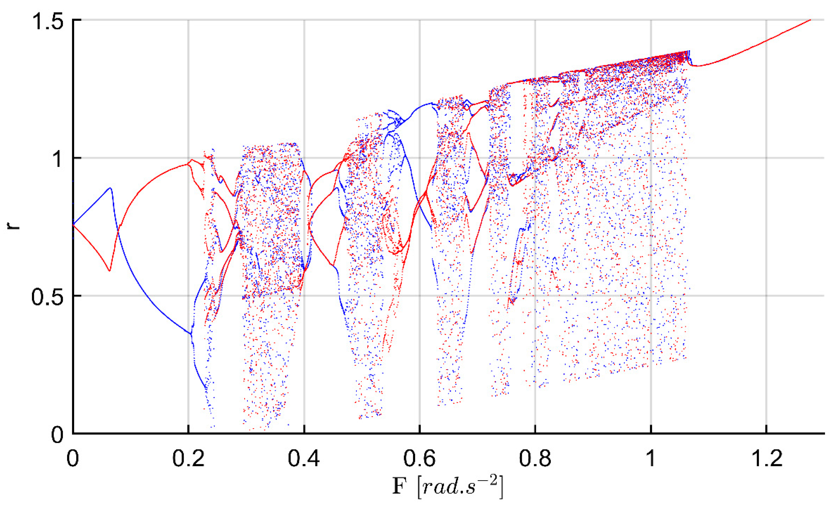
Figure 2 shows the stable and unstable roll motions based on the second iterative method, where r = ( x 1 2 + x 2 2 ) is the distance from the origin in the Poincaré map [32]. Unstable regions are more dominant as the forcing amplitude reaches 1. The ramp-up (blue line) and ramp-down parts (red line) enable checking the bistable region. Period-doubling routes to chaos and period-undoubling routes to single branches are clearly observed when the F increases [33]. With a slight increase in forcing amplitude, the periodic windows [11], which are stable regions, can be seen among the chaotic clouds of dots.
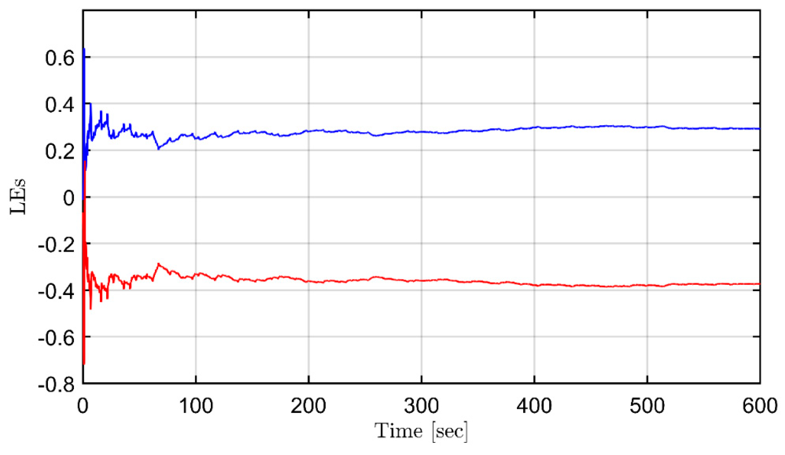
Figure 3 shows the Lyapunov exponents (LEs) of the uncontrolled system. The stretching and contracting of attractors are well defined by LEs, whose positive values signify chaos [11,34]. LE measures the mean rate of exponential divergence of nearby trajectories, which gives information on the growth rate of IC [20]. Positive LEs show that a roll system is sensitive to IC and trajectories will diverge within time evolution, while negative LEs indicate a convergence tendency. The larger the exponent, the more unstable the system. Particularly, a negative LE indicates that the system is stable [35]. Negative LEs are characteristics of dissipative systems such that the roll system exhibits asymptotic stability; the more negative the exponent, the greater the stability [36].
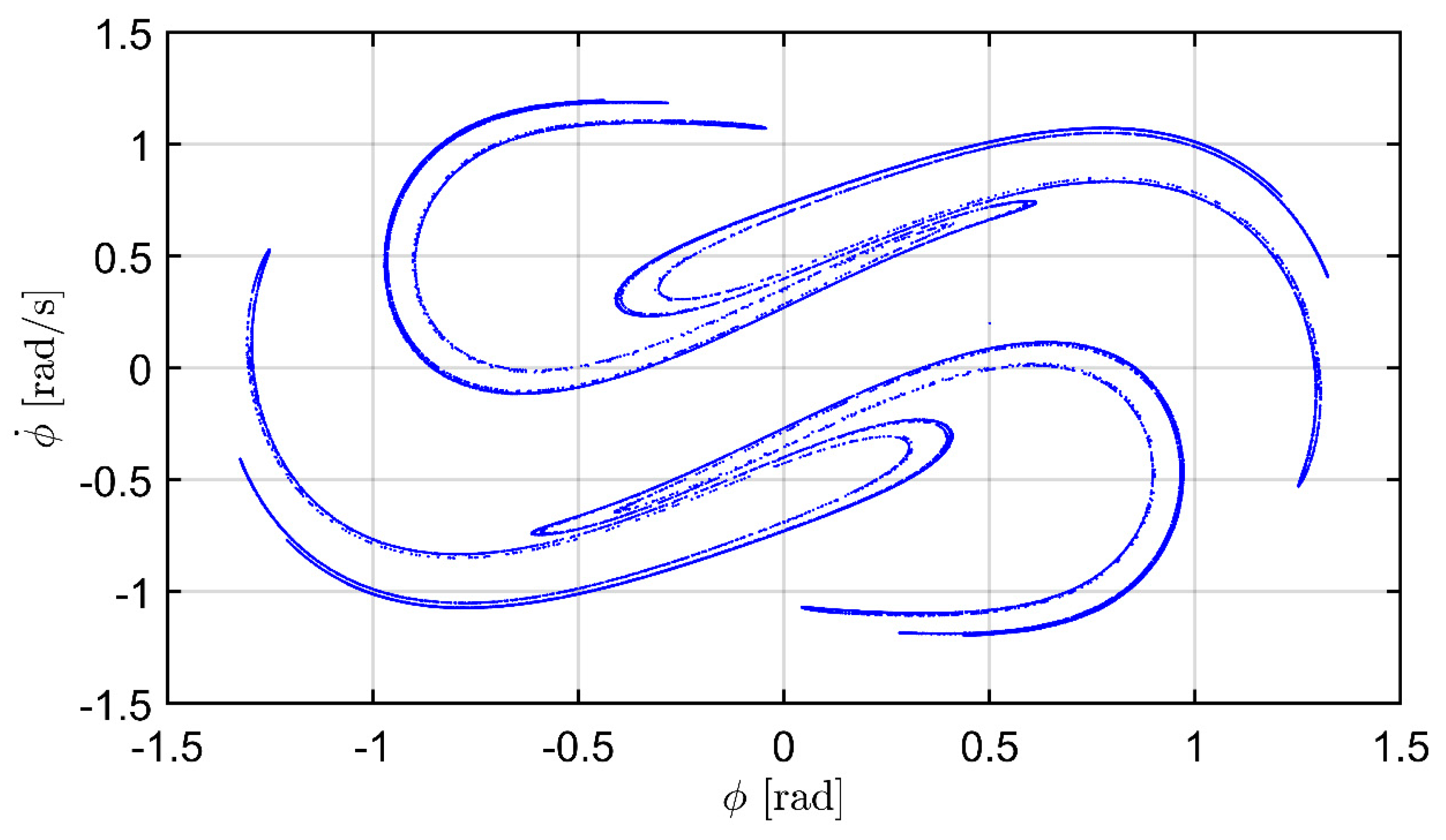
It appears to be nonperiodic, as seen in Figure 4, where the Poincaré section shows the uncontrolled roll of a deterministic system that has no random or noisy inputs [11]. The main parameters are adopted in a marine model [28], whereas the obscure values of IC are set to be changed only. The Poincaré map reduces the n-dimensional flow to a n 1 dimensional map [34]. All trajectories of an n-dimensional system starting on the n 1 dimensional surface of a section flow through it [11]. Such reduced dimensionality makes it possible to preserve periodic and quasi-periodic orbits [37]. To make an autonomous flow in a torus, a third value θ = Ω t can be considered from the equation (6) without control action. A trajectory flowing around a torus with period ( T = 2 π / Ω ) leads to the Poincaré mapping of a θ = θ 0 plane [32]. Picking up a cross-section of roll angle and rate, the Poincaré map is mainly varied according to the strength of the forcing function. The manifolds become tangent and intersect transversely when the F increases [38]. If a trajectory in the phase plane intersects itself repeatedly, then a strange attractor and fractals may be observed in the chaotic roll dynamics [39].

3.2. Prediction of chaotic roll motions using RC

Secondly, the chaotic roll motions are predicted via RC. Such an ESN algorithm is used to forecast the reference data of roll angle and roll rate for the training and prediction processes of the reservoir. After initializing input weight ( W i n ) and feedback weight ( W f b ) are fixed, the predicted process is performed from the computation of the trained reservoir. The elements of weights are withdrawn with the equal possibility in [ σ , σ ] , where σ means a hyper-parameter to adjust the performance [21]. The main parameter for prediction via RC is listed in Table 2. For example, the spectral radius and leaking rate, which relate to magnitude of the largest eigenvalue value of weight and performance, are set as ρ = 0.75, α = 0.08. The adjustment of the leaking rate ( α ) indicates the level of dependence of the network on past information. The lower α , the more dependent it is on past information [22,23]. The input range [ σ , σ ] indicates the dispersion level of components in weight matrices ( W i n , W f b ). As the α increases, the wider it spreads on the weight matrices. The author decides that α should not be too low because it will inflict an amplitude value on input and feedback responses.
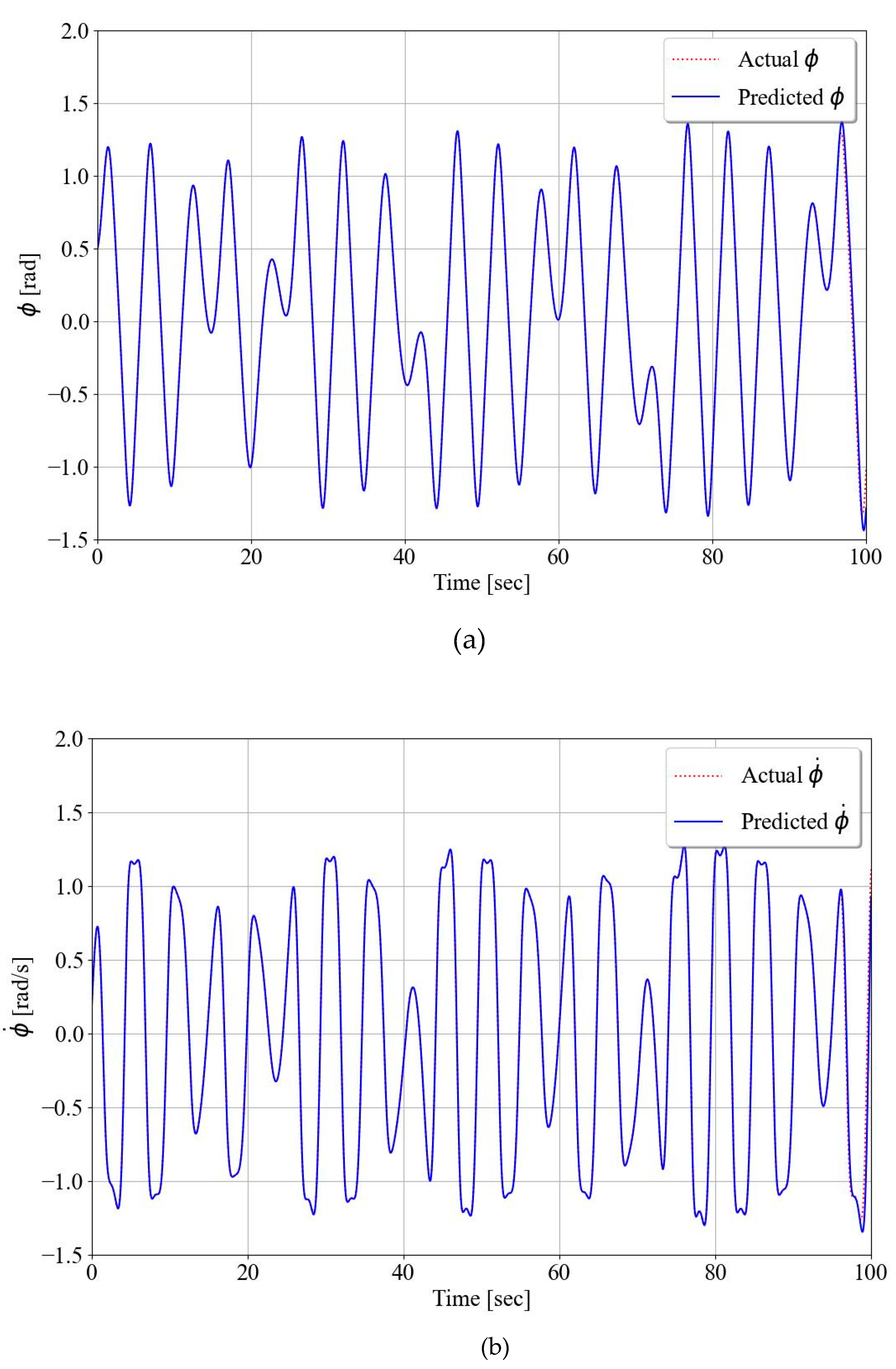
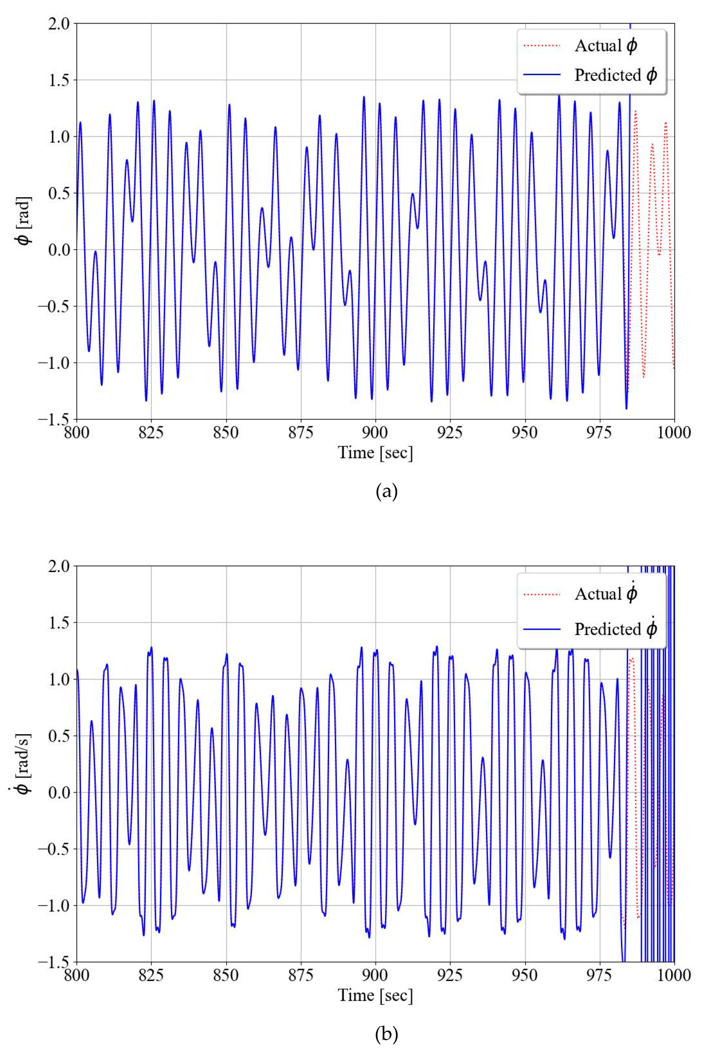
Figure 5 and Figure 6 show the results of chaos roll prediction, in which the roll angle and rate are trained until 95 and 980 seconds, respectively. Until the training time, the predicted values almost coincided with the actual behaviors in both Figs. 5 and 6. As for the short range of prediction, the values of MSE (mean-square error) for roll angle and rate are calculated as 0.0158 and 0.04169, respectively, as seen in Figure 5. To compare with the results of the uncontrolled chaotic roll angle in [28], we trained until 980 seconds in the case of Figure 6. As a result of the mention in the Introduction part, the RC process seems to be suitable even for long-term prediction of future states, even though the LEs show a lack of predictability [20].

3.3. Parametric identification of periodic disturbances

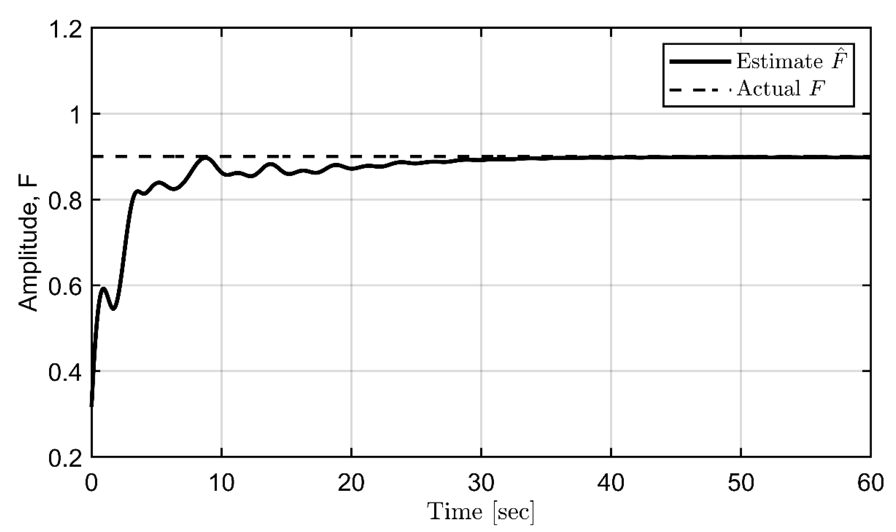
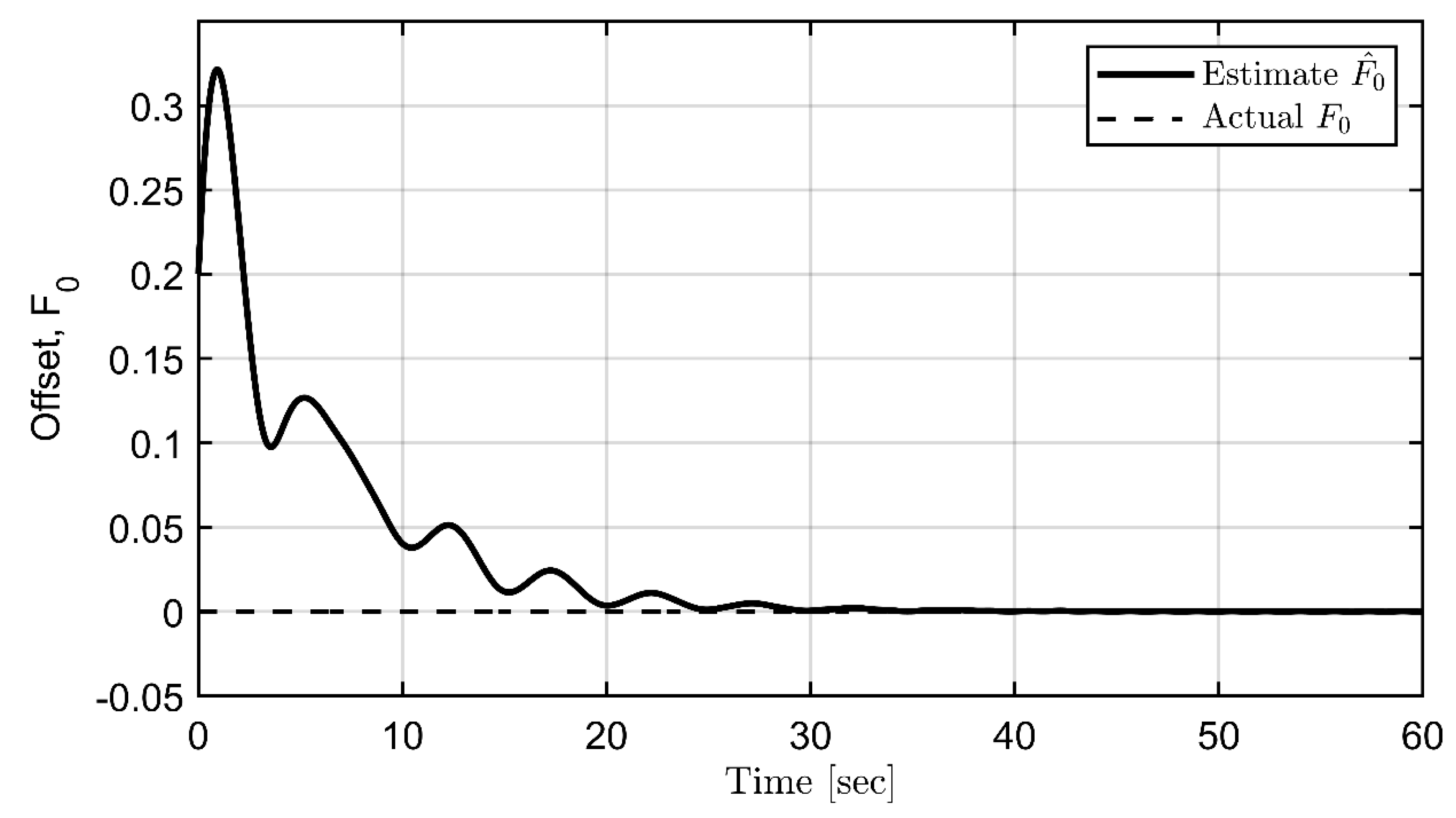
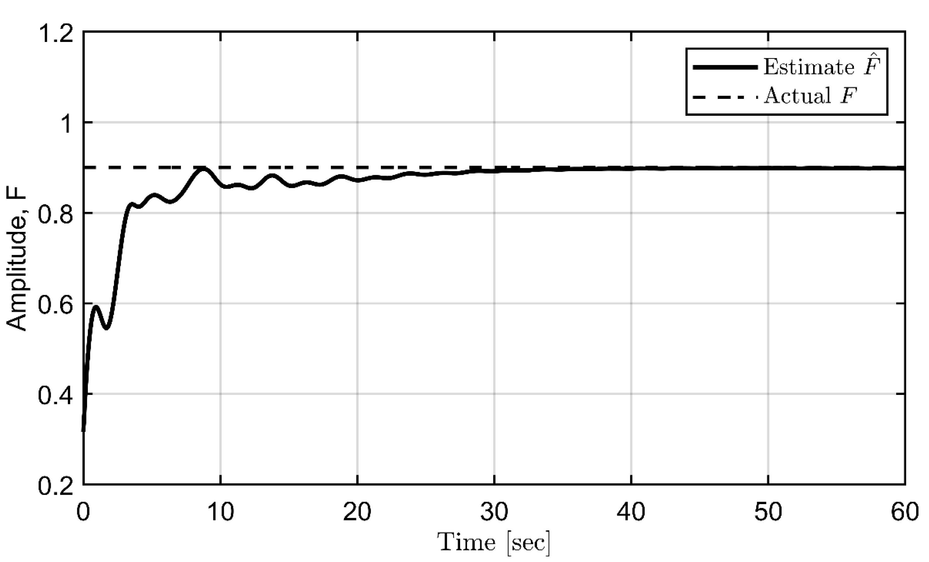
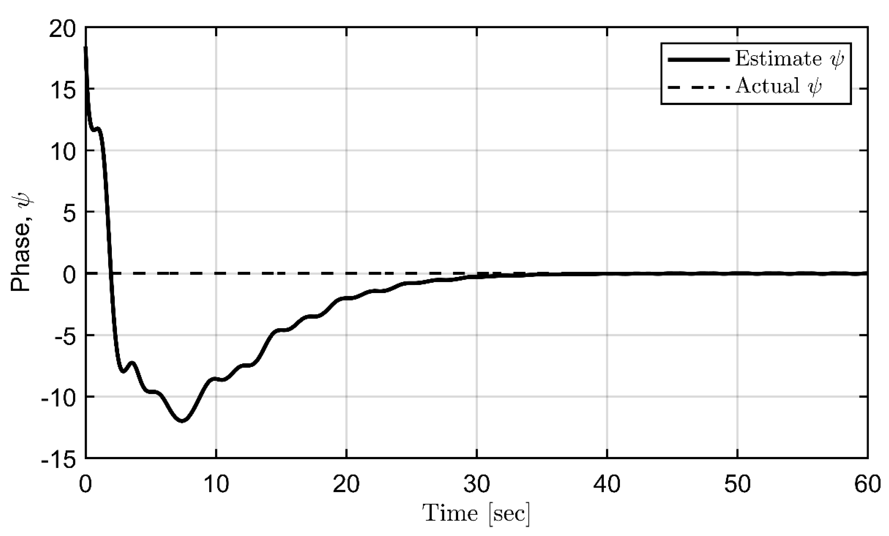
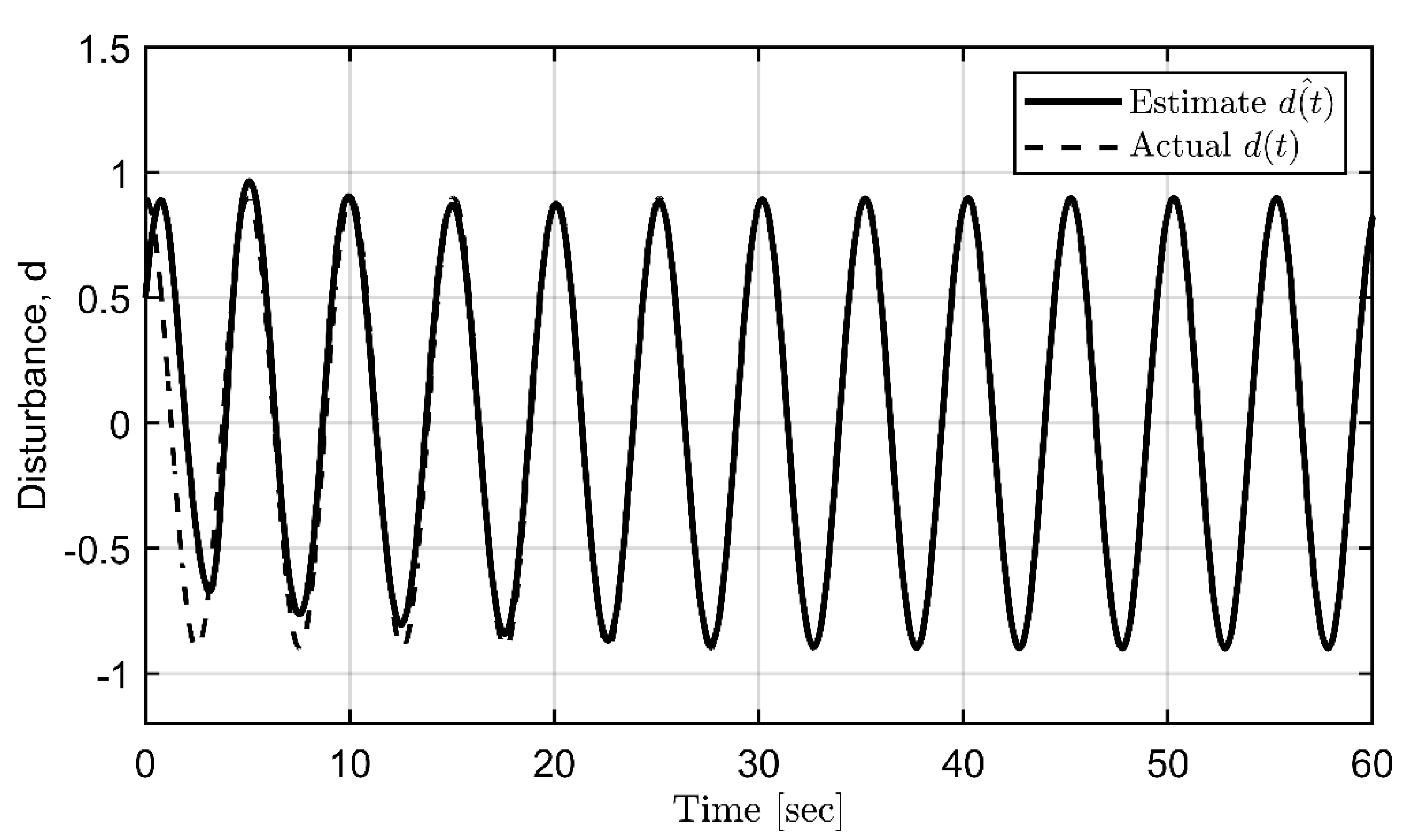
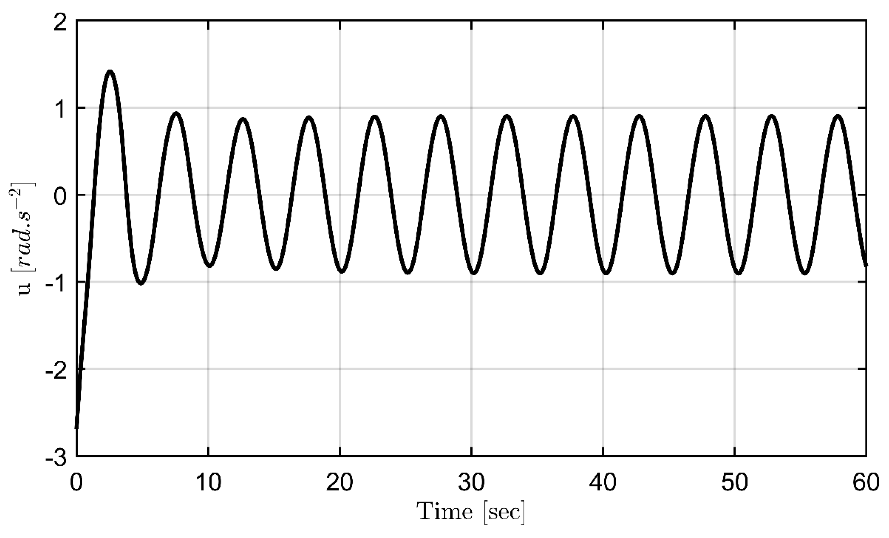
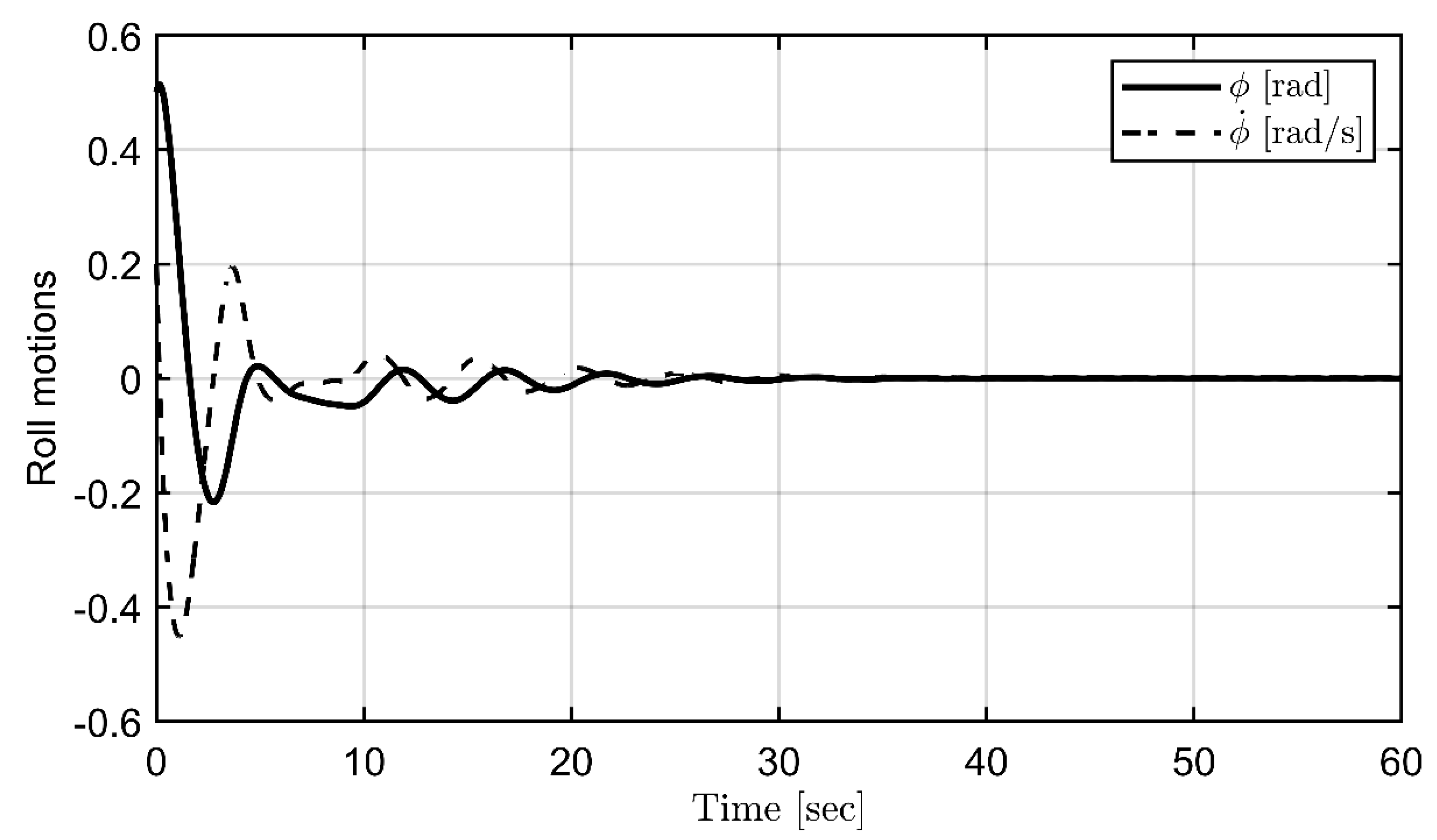
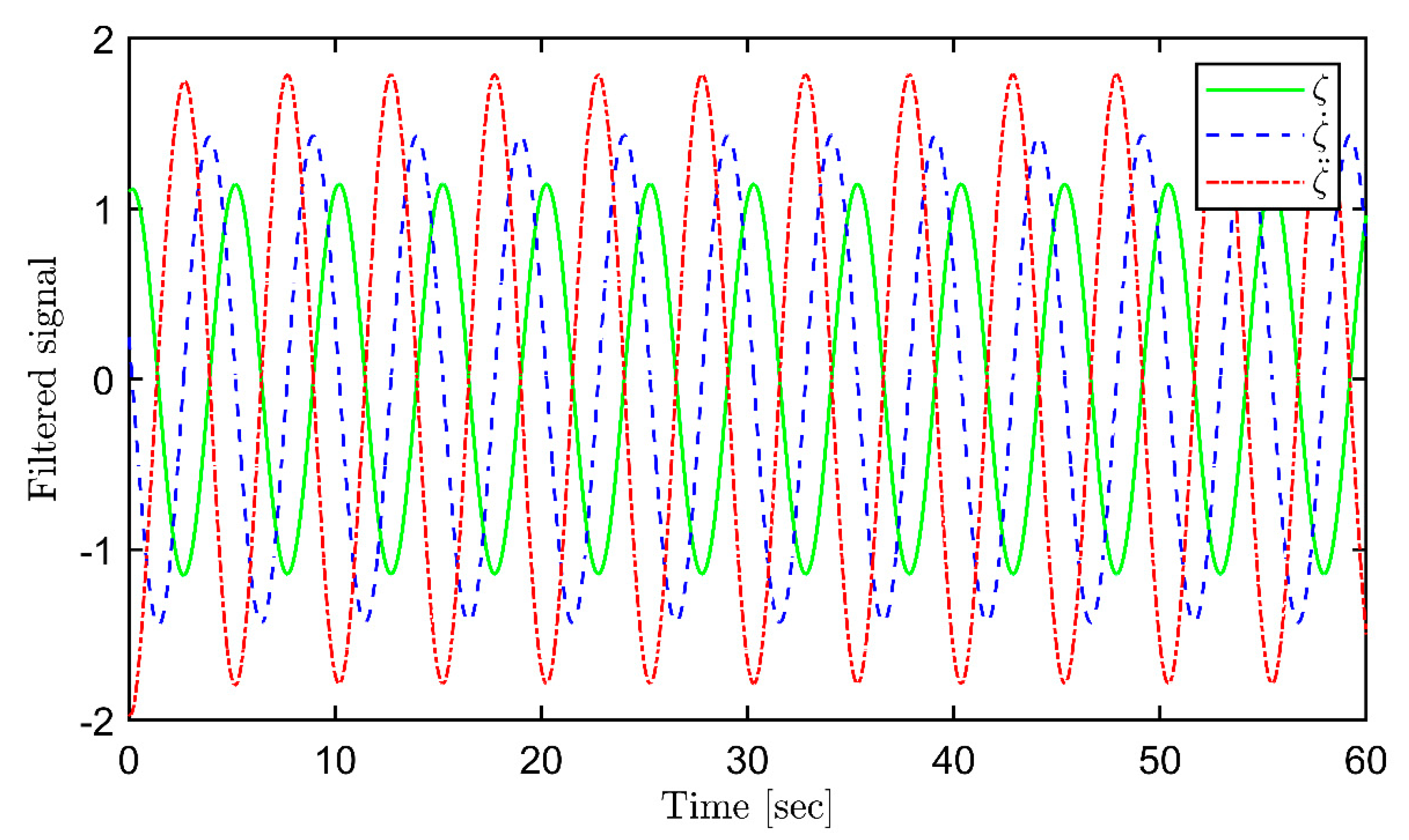
Finally, the simulations for the proposed backstepping control are conducted. The filter and controller design parameters are set as ( λ 0 , λ 1 , λ 2 , γ 1 , γ 2 , γ 3 ) = (0.15, 2, 8, 5, 5, 2.5). The update rate matrix is chosen as Γ 2 = d i a g ( 2 , 1.2 , 1.2 ) and the IC is ( F ^ o ( 0 ) , a ^ ( 0 ) , b ^ ( 0 ) , Ω ^ ( 0 ) ) = (0.2, 0.3, 0.1, 0). Figure 7, Figure 8, Figure 9 and Figure 10 demonstrate the estimation process for the frequency, offset, amplitude, and phase, respectively. In contrast, Figure 11 verifies a combination of the above results to form a complete estimation for the sinusoidal disturbance. All parameters of periodic disturbances can be precisely estimated. Suppression of roll angle and rate is achieved using the backstepping control, as seen in Figure 12 and 13. Finally, filtered signals are illustrated in Figure 14, according to the updated law in equation (17).

4. Conclusions

In this paper, parameter estimation and stabilization of unknown periodic disturbances are performed based on the adaptive mechanism without any observers. All parameters, such as frequency, offset, amplitude, and phase, were precisely estimated. The linear second-order filters and parameter estimation errors were used to achieve global exponential convergence. This paper has a limitation of slow convergence in transient performance; however, it sows less oscillation due to the second-order filtered signals as in [2,7]. So, more proper values should be set to make a tradeoff between fast convergence speed and transient performance. Also, the backstepping method was used to regulate the chaos roll angle and rate in the case of severe disturbances to marine vessels. Moreover, the RC process revealed its predictive performance of the long-term chaos behaviors; thus, it may help to support the lack of predictability of LEs [20]. To make a safe and robust system in the real world, it should be considered an adversarial attack based on adaptive control and the RL method [40] in the subsequent work.

Author Contributions

Conceptualization, S.S.Y.; methodology, L.N.B.L.; software, L.N.B.L.; validation, S.S.Y.; formal analysis, L.N.B.L.; investigation, B.D.H.P.; resources, S.D.L.; data curation, B.D.H.P.; Visualization, B.D.H.P.; writing—original draft preparation, S.D.L; writing—review and editing, H.S.K.; supervision, S.S.Y.; project administration, H.S.K.; Funding acquisition, H.S.K.; All authors have read and agreed to the published version of the manuscript.

Funding

This research was supported by the Korea Institute of Marine Science & Technology Promotion (KIMST) funded by the Ministry of Oceans and Fisheries, Korea (20220573).

Institutional Review Board Statement

Not applicable.

Informed Consent Statement

Not applicable.

Data Availability Statement

Not applicable

Conflicts of Interest

The authors declare no conflict of interest.

References

  1. Pyrkin, A.A.; Bobtsov, A.A.; Kolyubin, S.A.; Vedyakov, A.A. Precise frequency estimator for noised periodical signals. 2012 IEEE International Conference on Control Applications 2012, 92–97. [Google Scholar] [CrossRef]
  2. Na, J.; Yang, J.; Wu, X.; Guo, Y. Adaptive Parameter Identification of Sinusoidal Signals. IFAC Conference on Intelligent Control and Automation Science ICONS 2013, 46, 624–629. [Google Scholar] [CrossRef]
  3. Quinn, B.G.; Hannan, E.J. The Estimation and Tracking of Frequency: Cambridge Univ. Press: Cambridge, U.K, 2001. [CrossRef]
  4. Hou, M. Parameter identification of sinusoids. IEEE Transactions on Automatic Control 2012, 57, 467–472. [Google Scholar] [CrossRef]
  5. Slotine, J.J.E.; Li, W. Applied nonlinear control; Prentice Hall Englewood Cliffs: NJ, 1991. [Google Scholar]
  6. Lin, J.-S.; Kanellakopoulos, I. Nonlinearities enhance parameter convergence in output-feedback systems. IEEE Trans. Autom. Control. 1998, 43, 204–222. [Google Scholar] [CrossRef]
  7. Na, J.; Yang, J.; Wu, X.; Guo, Y. Robust adaptive parameter estimation of sinusoidal signals. Automatica 2015, 53, 376–384. [Google Scholar] [CrossRef]
  8. Yilmaz, C.T.; Basturk, H.I. Output feedback control for unknown LTI systems driven by unknown periodic disturbances. Automatica 2018, 99, 112–119. [Google Scholar] [CrossRef]
  9. Na, J.; Mahyuddin, M.N.; Herrmann, G.; Ren, X.; Barber, P. Robust adaptive finite-time parameter estimation and control for robotic systems. Int. J. Robust Nonlinear Control. 2014, 25, 3045–3071. [Google Scholar] [CrossRef]
  10. Adetola, V.; Guay, M. Performance Improvement in Adaptive Control of Linearly Parameterized Nonlinear Systems $ $. IEEE Trans. Autom. Control 2010, 55, 2182–2186. [Google Scholar] [CrossRef]
  11. Strogatz, S. H. Nonlinear Dynamics and Chaos: With Applications to Physics, Biology, Chemistry, and Engineering; CRC Press, 2018. [Google Scholar]
  12. Jiménez-Casas. ; Castro, M.; Villanueva-Pesqueira, M. The Role of Elasticity on Chaotic Dynamics: Insights from Mechanics, Immunology, Ecology, and Rheology. Mathematics 2023, 11, 3099. [Google Scholar] [CrossRef]
  13. Ott, E.; Grebogi, C.; Yorke, J.A. Controlling chaos. Phys. Rev. Lett. 1990, 64, 1196–1199. [Google Scholar] [CrossRef]
  14. Y. Tang, J. Y. Tang, J. Kurths, W. Lin, E. Ott, L. Kocarev. Introduction to Focus Issue: When machine learning meets complex systems: Networks, chaos, and nonlinear dynamics. Chaos 2020, 30, 063151. [Google Scholar] [CrossRef] [PubMed]
  15. Jaeger, H. , 2001. The echo state approach to analyzing and training recurrent neural networks., Tech. rep., GDM 148, German national resource center for information technology.
  16. Lukoševičius, M.; Jaeger, H. Reservoir computing approaches to recurrent neural network training. Comput. Sci. Rev. 2009, 3, 127–149. [Google Scholar] [CrossRef]
  17. Jaeger, H.; Haas, H. Harnessing Nonlinearity: Predicting Chaotic Systems and Saving Energy in Wireless Communication. Science 2004, 304, 78–80. [Google Scholar] [CrossRef] [PubMed]
  18. LeCun, Y.; Bengio, Y.; Hinton, G. Deep learning. Nature 2015, 521, 436–444. [Google Scholar] [CrossRef]
  19. Ferreira, A.A.; Ludermir, T.B.; de Aquino, R.R. An approach to reservoir computing design and training. Expert Syst. Appl. 2013, 40, 4172–4182. [Google Scholar] [CrossRef]
  20. Boffetta, G.; Cencini, M.; Falcioni, M.; Vulpiani, A. Predictability: a way to characterize complexity. Phys. Rep. 2002, 356, 367–474. [Google Scholar] [CrossRef]
  21. Long, L.N.B.; Cuong, T.N.; Kim, H.-S.; You, S.-S. Sustainability and robust decision-support strategy for multi-echelon supply chain system against disruptions. Int. J. Logist. Res. Appl. 2023, 1–31, Available at SSRN: https://ssrn.com/abstract=4020779. Int. J. Logist. Res. Appl. 4020; 31. [Google Scholar] [CrossRef]
  22. Lukoševičius, M. A Practical Guide to Applying Echo State Networks. In: Montavon, G., Orr, G.B., Müller, KR. (eds) Neural Networks: Tricks of the Trade. Lecture Notes in Computer Science, vol 7700. Springer, Berlin, Heidelberg. 2012. [Google Scholar] [CrossRef]
  23. Herbert Jaeger, 2007. Echo state network. Scholarpedia, 2(9):2330. http://www.scholarpedia.org/article/Echo_state_network.
  24. Zhou, J.; Wen, C. Adaptive Backstepping Control. In: Adaptive Backstepping Control of Uncertain Systems. Lecture Notes in Control and Information Sciences, vol 372. Springer, Berlin, Heidelberg. 2008; 31. [Google Scholar] [CrossRef]
  25. Lee, S.-D.; Song, Y.-S.; Kim, D.-H.; Kang, M.-R. Path following Control of an Underactuated Catamaran for Recovery Maneuvers. Sensors 2022, 22, 2233. [Google Scholar] [CrossRef]
  26. Jeong, G.-S.; Lee, S.-J. Autonomous surveillance maneuvers for marine vessels in specially designated waters with a focus on the consecutive port and starboard turning cases. J. Korean Soc. Mar. Eng. 2022, 46, 237–247. [Google Scholar] [CrossRef]
  27. Lee, S.-D.; You, S.-S. Dynamical Rolling Analysis of a Vessel in Regular Beam Seas. J. Korean Soc. Mar. Environ. Saf. 2018, 24, 325–331. [Google Scholar] [CrossRef]
  28. Lee, S.-D.; Phuc, B.D.H.; Xu, X.; You, S.-S. Roll suppression of marine vessels using adaptive super-twisting sliding mode control synthesis. Ocean Eng. 2019, 195, 106724. [Google Scholar] [CrossRef]
  29. Lee, S.-D.; You, S.-S.; Xu, X.; Cuong, T.N. Active control synthesis of nonlinear pitch-roll motions for marine vessels. Ocean Eng. 2021, 221, 108537. [Google Scholar] [CrossRef]
  30. Lee, S.D., You, Sam-Sang, Long, Le Ngoc Bao, Phuc, Bui Duc Hong. 2022. Active control for parametric instability and resonance of container ship model. available at SSRN: https://ssrn.com/abstract=4239145. 4239.
  31. P.A. Ioannou, J. P.A. Ioannou, J. Sun, 1996. Robust adaptive control, Upper saddle river, NJ: Prentice hall. 78.
  32. Lynch, S. Poincaré Maps and Nonautonomous Systems in the Plane. In: Dynamical Systems with Applications using MATLAB®. Birkhäuser, Cham. 2014. [Google Scholar] [CrossRef]
  33. Lynch, S. Electromagnetic Waves and Optical Resonators. In: Dynamical Systems with Applications using MATLAB®. Birkhäuser, Cham. 2014. [Google Scholar] [CrossRef]
  34. Ott, E. Chaos in Dynamical Systems. (2nd ed.). Cambridge: Cambridge University Press. 2002. [Google Scholar] [CrossRef]
  35. Dey, K.K.; Sekh, G.A. Effects of Random Excitations on the Dynamical Response of Duffing Systems. J. Stat. Phys. 2021, 182, 1–14. [Google Scholar] [CrossRef]
  36. BenSaïda, A. A practical test for noisy chaotic dynamics. SoftwareX 2015, 3-4, 1–5. [Google Scholar] [CrossRef]
  37. Bramburger, J.J.; Kutz, J.N. Poincaré maps for multiscale physics discovery and nonlinear Floquet theory. Phys. D: Nonlinear Phenom. 2020, 408, 132479. [Google Scholar] [CrossRef]
  38. Guckenheimer, J.; Holmes, P. An Introduction to Chaos: Four Examples. 1983, 66–116, In: nonlinear oscillations, dynamical systems, and bifurcations of vector fields. Applied Mathematical Sciences, vol 42. Springer, New York, NY. [CrossRef]
  39. Grebogi Celso, Ott Edward, Yorke James A. Chaos, strange attractors, and fractal basin boundaries in nonlinear dynamics". Science 1987, 238, 632–638. [CrossRef]
  40. Annaswamy, A.M. Adaptive Control and Intersections with Reinforcement Learning. Annu. Rev. Control. Robot. Auton. Syst. 2023, 6, 65–93. [Google Scholar] [CrossRef]
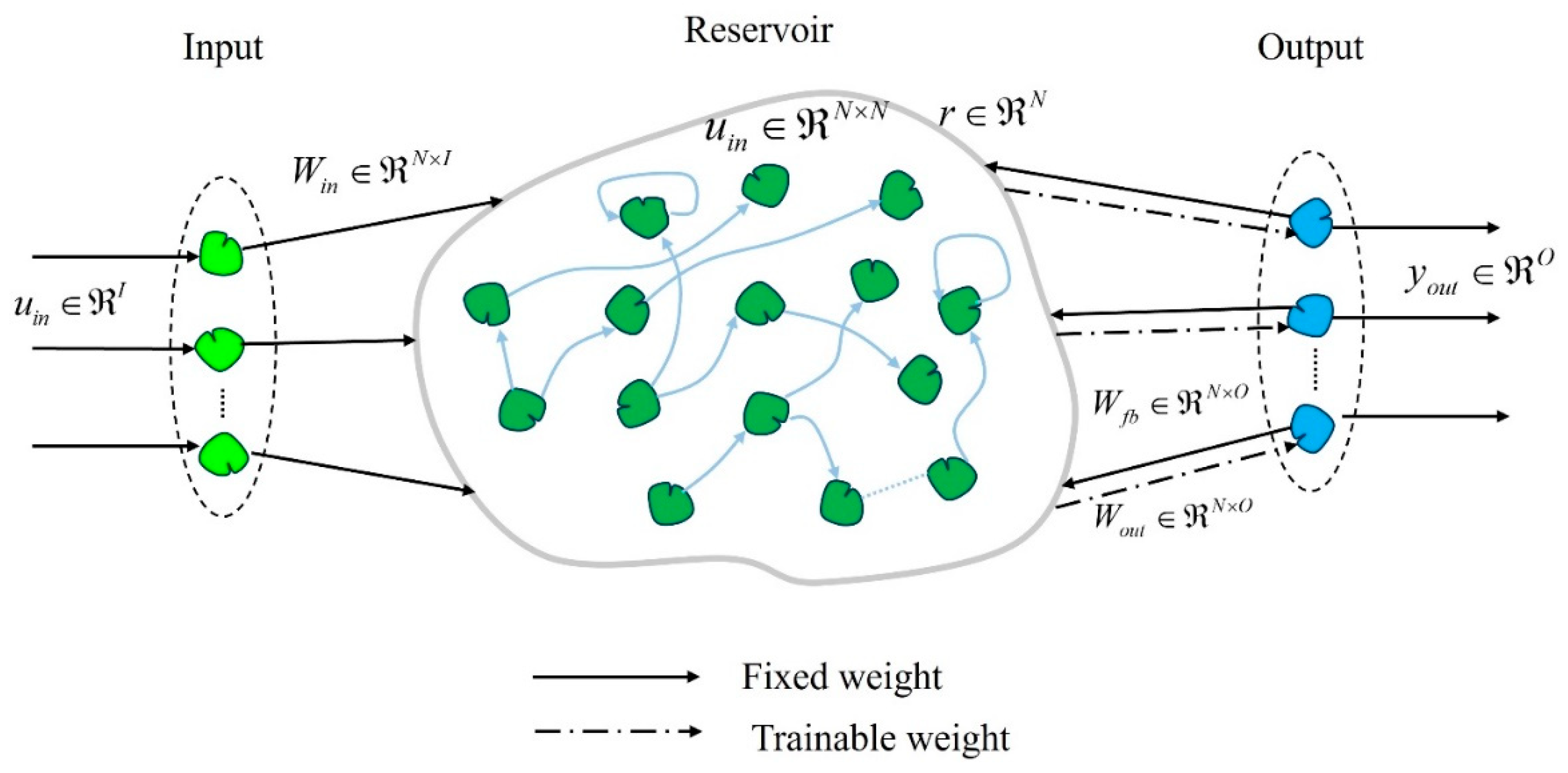
Figure 1. Generic structure of RC framework [21].
Preprints 83575 g001
Figure 2. Bifurcation diagram using the second iterative method.
Preprints 83575 g002
Figure 3. Lyapunov exponents of the uncontrolled system with IC [0.5 (rad) 0.2(rad/s)].
Preprints 83575 g003
Figure 4. Poincaré section of the uncontrolled system with IC [0.5 (rad) 0.2(rad/s)].
Preprints 83575 g004
Figure 5. Prediction of roll angle (a) and roll rate (b) for 100 seconds. Training until 95 seconds.
Preprints 83575 g005
Figure 6. Prediction of roll angle (a) and roll rate (b) for 1000 seconds. Training until 980 seconds.
Preprints 83575 g006
Figure 7. Estimated frequency.
Preprints 83575 g007
Figure 8. Estimated offset.
Preprints 83575 g008
Figure 9. Estimated amplitude.
Preprints 83575 g009
Figure 10. Estimated phase.
Preprints 83575 g010
Figure 11. Complete estimation for disturbances.
Preprints 83575 g011
Figure 12. Control input activity.
Preprints 83575 g012
Figure 13. Controlled roll motions.
Preprints 83575 g013
Figure 14. Filtered signals.
Preprints 83575 g014
Table 1. Details of a chaotic marine model.
Parameters Value
Non - dimensional   value   ( b 1 ) 0.081
Non - dimensional   value   ( b 2 ) 0.419
Non - dimensional   value   ( k 2 ) 1.746
Table 2. Main parameters of prediction via RC [21].
Parameters Value
Leaking rate ( α ) 0.08
Spectral radius ( ρ ) 0.75
Range of input ( σ ) 0.5
Disclaimer/Publisher’s Note: The statements, opinions and data contained in all publications are solely those of the individual author(s) and contributor(s) and not of MDPI and/or the editor(s). MDPI and/or the editor(s) disclaim responsibility for any injury to people or property resulting from any ideas, methods, instructions or products referred to in the content.
Copyright: This open access article is published under a Creative Commons CC BY 4.0 license, which permit the free download, distribution, and reuse, provided that the author and preprint are cited in any reuse.
Prerpints.org logo

Preprints.org is a free preprint server supported by MDPI in Basel, Switzerland.

Subscribe

© 2024 MDPI (Basel, Switzerland) unless otherwise stated