Preprint

Article

Multivariate Analysis for Prediction of Splitting Tensile Strength in Concrete Paving Blocks

Altmetrics

Downloads

Views

Comments

A peer-reviewed article of this preprint also exists.

Vinicio Ramiro Benalcázar-Rojas^*

Wilman Jenny Yambay-Vallejo^*,

Erick Patricio Herrera-Granda^*

Vinicio Ramiro Benalcázar-Rojas^*

Wilman Jenny Yambay-Vallejo^*,

Erick Patricio Herrera-Granda^*

This version is not peer-reviewed

Submitted:

29 August 2023

Posted:

31 August 2023

You are already at the latest version

Alerts

Abstract

Paving blocks are concrete pieces placed in exposed places to the weather, which are sub-jected to loads and wear. Hence, quality control in the manufacture of paving blocks is es-sential to guarantee the properties and durability of the product in construction projects. In Ecuador, the requirements are described in the Ecuadorian technical standard "NTE INEN 3040", and tensile splitting strength is a fundamental requirement to guarantee product quality. It is analyzed using quality control measurements such as dimensions, the weight of the fresh paving block in the vibro-compacted process, and the percentage of water absorption in order to know how the variables influence and manage to predict the tensile splitting strength to avoid product non-conformity in advance, having a timely and better control of the manufacturing process. The data was obtained from a company that can produce 30 000 units per day of rectangular paving blocks with 6 cm thickness. Mul-tivariate models such as multiple linear regression, regression trees, random forests and neural networks are performed to predict the tensile splitting strength variable through two groups of predictors; the first group is the thickness mm, width mm, length mm, mass of fresh paving block g and percentage of water absorption %. The second group of pre-dictor variables is the density of the fresh paving block kg/m3 and the percentage of water absorption %. It is concluded that the multiple linear regression method performs better in predicting the first group of predictor variables with a mean square error (MSE) of 0.110086, followed by the neural network without hidden layers resulting in an MSE of 0.112198. The best method for the second set of predictors was the neural network with-out hidden layers with a mean square error ( MSE ) of 0.112402, closely followed by the multiple linear regression model with an MSE of 0.115044.

Keywords:

Subject: Engineering - Industrial and Manufacturing Engineering

1. Introduction

Concrete is a mixture of water, cement, and aggregates with or without additives, whose hardening action allows it to be used in multiple applications; the standard defines it [1] as a material composed of a binding component with embedded particles and aggregates. One of its uses is manufacturing moulded pieces with defined dimensions called paving blocks, which are intended to be used generally in streets, parking lots, sidewalks, and parks. The batch-type paving blocks manufacturing process involves mixing, vibro-compacting, curing and palletizing. In process control and continuous improvement, a company with high production volumes in Quito -Ecuador, has quality controls with specialists in raw materials, intermediate goods and finished goods for each batch of 30 000 paving blocks. The vibro-compacting machine compacts the mixture that enters the mould and uses a tamper that shapes the fresh paving blocks, for which the dimensions, the weight of the vibro-compacted paving block and the water absorption test are means of controlling the product.

The tensile splitting strength test described in the standard [2], previously called “essai brésilien”, appeared in Brazil during the Second World War, being its scope and utility in concrete cylinders. The determination of the resistance to compression in concrete paving blocks is described in the norm [3] of the Servicio Ecuatoriano de Normalización; however, this norm was replaced by the norm [1] that indicates the test methods and requirements for concrete paving blocks, where the compressive strength test is omitted occupying the tensile splitting strength test. The standard [1] is based on the Spanish standard UNE EN 1338:2004. The article described by [4] indicates how the paving blocks break on-site in their daily use, not by compression but by fracture (splitting); for this reason, the tensile splitting strength test is recommended to measure its ability to resist stresses.

The tensile splitting strength is the variable with the most significant attention for customers and the commercial area since it indicates the breaking point of the material and its useful life on site. The test is carried out 28 days after its manufacture, which is why the problem arises in ignoring this characteristic at the initial age of the paving block when it is manufactured and the need to predict the tensile splitting strength in advance to avoid nonconforming paving blocks due to limited vision regarding this property. Consequently, knowing how the tensile splitting strength (called dependent or response variable) depends on the control variables in the vibro-compacting process and water absorption test (called explanatory, independent or predictors variables) will allow us to perform the prediction with an acceptable error statistically, making models and checking the structural assumptions defined in the literature.

This article aims to predict the tensile splitting strength through the quality control variables of the vibro-compacting process and the water absorption test of paving blocks. A statistical sampling is carried out to infer 30 000 units of the rectangular paving block with 6 cm of thickness (study population) representing a production batch. Specific objectives include identifying the main multivariate techniques based on the case study, implementing multivariate models in various configurations and methodologies to predict the response variable, comparing their benefits and limitations, and determining the best model to predict tensile splitting strength.

In order to carry out the correct statistical analysis for the prediction of a continuous dependent variable using multiple continuous explanatory variables, a set of hypotheses must be verified and inferred to the study population, carrying out adequate sampling, processing of the database using an analysis of atypical data, modelling and verification of assumptions.

Related work

The related studies for the prediction of tensile splitting strength are diverse due to the different areas of interest and possibilities, such as the study carried out by [5], which relates the tensile splitting strength with each of the variables through simple linear regression (the compressive strength, W/B ratio (water/binder) and the age of the concrete). Considering the criteria and formulas of the bibliographic review where tensile splitting strength is related to compression and the different prediction methods are compared. As the compressive strength increases, the tensile splitting strength also increases, observing that the water/binder ratio and age influence the strength development. It was concluded that tensile splitting strength is a function of parameters such as compressive strength, water/binder ratio, and age in different simple linear regression models. Equations were proposed for the prediction giving a non-linear relationship where tensile splitting strength increases more slowly than compression.

In Turkey, the study by [6] indicates that abrasion resistance with Bohme testing and split strength are two of the most important properties for determining the quality of concrete paving blocks. These properties are related to dry bulk specific gravity and the ultrasonic pulse velocity with the “PUNDIT” equipment that measures the time of passage of ultrasound waves when passing through the thickness of the paving stone. Samples are taken from seven paving block manufacturers. It is verified that there is a greater dependence of split strength with the dry bulk specific gravity using a logarithmic transformation giving a determination coefficient of 0.59 with significant coefficients.

An investigation is carried out by [7] in Hong Kong where different mixtures are prepared, the first with 100% recycled concrete aggregate, the second incorporating crushed tile, the third incorporating crushed tile and glass, the fourth crushed brick and tile in different proportions, the fifth used crushed tile, brick and glass, the sixth mix incorporate crushed brick, glass, tile and wood chips. The paving block mould was 20 cm x 10 cm x 6 cm. The results mainly concluded that the compressive strength increases with the increase in density, the water absorption decreases with increasing density, the compressive strength increases with the aggregate/cement ratio, and the contamination level in the aggregate can be a maximum of 10%.

The study that was carried out by [4] explains the water absorption test and additionally indicates that the compression test described in Standard NS 6717:1986, which is carried out in the laboratory, does not represent the real behaviour in the paving blocks in real conditions of use, and it is caused by splitting stresses. For this reason, it is more advisable to carry out the tensile splitting strength described in the BS EN 1338 standard, which generates a fracture by dividing the paving block into two parts. Compressive and tensile splitting strengths are also related, establishing dependency equations between these variables.

The investigation carried out by [8] to predict the tensile splitting strength in concrete indicates that the compressive strength and tensile strength are essential characterization indices of the concrete, indicating that generally, the compressive strength is much lower than the tensile strength, the study proposes an alternative method to predict the tensile splitting strength by compressive strength using a novel method called GEP which is a gene expression programming technique for developing programs and is based on constantly adapting tree structures.

The article written by [9] is based on the realization of different mixtures with different amounts of rubber and water/cement ratios determining the density of the concrete according to the BS 6717 standard, simple linear and logarithmic regressions are created relating the density with the percentage of rubber, in the same way for the compressive strength and the study concludes that an increase in the content of rubber produces a reduction in resistance and density. It is worth mentioning that, in the results table, the lowest compressive strength occurs in cases where density is lower. In the same way, the highest compressive strength is observed in cases where density is higher for the same ratio of water/cement.

The different regression methods were studied by [10], such as neural networks and gene expression programming to predict splitting tensile strength and water absorption using predictor variables such as the amount of cement, amount of ZnO2 nanoparticles, type of aggregate, content of water, amount of superplasticizer, age and cured type and number of test attempts with various types of concrete including ZnO2 nanoparticles. The training and validation data are separated to perform two models with different design parameters. The determination coefficients for the relationship between predicted values and values of the validation set are: a) For the two neural network models, the prediction of splitting tensile strength are 0.9209 and 0.9249 and for water absorption, 0.9479 and 0.9652. b) For the two models using gene programming, the prediction of splitting tensile strength is 0.9093 and 0.9412, and for water absorption is 0.9313 and 0.9459.

The prediction by multiple linear regression of the compressive strength can be seen in the study carried out by [11], where it is indicated that incorporating rubber from vehicular transport tires in the paving block mixture and replacing it with a certain percentage of aggregate, the compressive and traction strength decreases. It was also indicated that a good water/cement ratio (W/C) significantly improves the properties of concrete, and models derived from experimental results were established to predict the density and compressive strength of paving blocks. The density was calculated using the BS 1881 standard, and the compressive strength was calculated by the failure load by the area. The density decreased with increasing rubber in the mix; the compressive strength increased as the amount of rubber increased. Multiple regression analysis is carried out in the SPSS program version 16, establishing the water/cement ratio and the amount of rubber as independent variables. The model made for the prediction of compressive strength indicates a determination of coefficient R² = 0.992, so 99.2% of the variation in compressive strength can be explained by the independent variables.

The research led by [12] used 200 x100x100 paving blocks manufactured by vibro-compaction; the objective was to determine the changes in density using the DIN12390-7 standard, absorption, freezing–thawing resistance and tensile splitting strength of paving blocks on the pallet. The values of the coefficients of variation are 1.4% for density, 15.6% for tensile strength, for freezing–thawing resistance is 3.7%, for abrasion resistance it is 2.7%. It is indicated that the changes at the ends of the tray were attributable to the uneven distribution of the compaction and filling of the mixture in the vibro-compacting machine, making the density higher in the centre and lower at the ends. Likewise, when the density is lower at the ends, the product’s resistance is lower.

The authors [13] delved into preparing concrete mixes with different water/cement ratios in cubes, subjecting them to different curing methods, sorptivity test, the height of permeability, water absorption and compressive strength were measured. It resulted in curing in an environment with a relative humidity of 90% +-5% 20+-3 degrees Celsius the most minor absorption. The authors indicated no clear relationship between compressive strength and water absorption.

The relationship of different physical and mechanical properties of concrete paving blocks for 112 samples in Albania was carried out by [14], where it is described as physical variables: the water absorption, porosity and specific gravity according to the BS EN 1338:2003 standard, and as mechanical variables: compressive strength and tensile splitting strength. The regressions of the variables were carried out, where it was found that the most robust correlation coefficients are: a) correlation between the water absorption and the tensile splitting strength, b) the compressive strength and the water absorption, c) porosity and compressive strength, d) porosity and tensile splitting strength. Additionally, it is indicated that water absorption is a physical property that can be easily determined, has a high correlation with performance parameters, and can also be used as a rapid quality control parameter.

In the investigation carried out by [15], several concrete mixtures with different densities and water/cement ratios were elaborated in order to be able to relate them with the resistance at 28 days of age. The increase in the density of the concrete increased the compressive strength with an exponential behaviour and a coefficient of determination greater than 0.9.

The study described by [16]incorporates tea waste ash with different proportions to replace cement, giving us a lower density and compression with a higher proportion of ash. It can be seen in the graphs of this study that the first two mixtures with the minor cement replacement give us the highest compressive strength, and these same samples are the ones with the highest density.

In Indonesia, the study carried out by [17]uses different ratios of NaOH/Na2SiO3 and fly ash as a substitute for cement in order to predict the performance of paving blocks, higher Na2SiO3 content results in lower percentage absorption and higher endurance.

In another investigation carried out in Indonesia, different mixtures were elaborated to study the behaviour of the paving blocks, [18] details that two groups were compared; the first group incorporates only sand and the second gravel (stone). It was indicated that a high-quality paving block has a high compressive strength and low water absorption percentage. The results show that the resistance of the paving block only with sand gives greater resistance.

In the study carried out by [19], 40 types of methods for data analysis are summarized and discussed with an approach to pavement engineering for prediction and classification of variables; the models include linear and non-linear regression, logistic regression, count data model, survival analysis, stochastic processes, time series, significance tests, design of experiments, neural networks, decision trees, ensemble learning, support vector machines, instance-based learning, discriminant analysis, principle component analysis, factor analysis, cluster analysis, structural equation modelling, Bayesian, reinforcement learning. They delved into the data analysis, explaining in detail the definition of each one, being the regression models understandable and easy to interpret as linear and non-linear equations, logistic regression, survival analysis and stochastic processes, giving the coefficients of regression a quantitative meaning. Supervised machine learning models: artificial neural networks, decision trees, support vector machine, and k-nearest neighbours give the ability to predict and classify large volumes of data.

A comparison of performance measures is carried out in the study carried out by [20] in China for the prediction of resistance in high-performance concrete, dividing the database into training and validation to apply the machine learning methods: Random Forest (RF), Support Vector Regression (SVR) and the XGBoost algorithm. Giving us the lowest mean square error with the XGBoost method, the prediction results ranged from 20 MPa to 70 MPa, taking as input variables the use of cement, age, coarse aggregate, fine aggregate, water reduction, fly ash and mineral powder. The coefficient of determination of the three models was above 0.9.

The elaboration of different mixtures incorporating wheat straw fibres with and without treatment with sodium silicate was studied by [21], whose results of the properties in the concrete paving blocks allowed to conclude that the untreated mixtures increased the percentage of water absorption and decreased the compressive strength and tensile splitting strength. In this study, it can be seen from the graphs that the mixture with the lowest compressive strength and tensile splitting strength is the one with the highest percentage of water absorption.

The artificial neural network, decision trees and random forest methods for predicting tensile splitting strength were described in the study by [22], where concrete is used as a recycled aggregate, obtaining the database divided into training and validation. The input variables were the amount of water, cement, superplasticizer, fine aggregate, coarse aggregate, residual coarse aggregate, density, and water absorption. The random forest method showed a higher coefficient of determination when relating the predicted values and the validation base; additionally, it gave lower error values than the other methods.

2. Materials and methods

The paving blocks of the present investigation were obtained from a factory that produces 30 000 units per day in Quito - Ecuador; the paving block model is rectangular with nominal dimensions of length 200 mm, 100 mm in width and 60 mm in thickness. The research has a quantitative approach since all the variables to be analyzed are continuous quantitative.

As a first point, the sample size is estimated using the G* Power software for multiple linear regression of 5 predictors, using a medium range effect size of 0.0363, which allowed estimating a sample size of 300 paving stones, with which an estimated power of the test of 0.9502764 was obtained. On production day, the paving blocks for the population of 30 000 units are sampled as the pieces come out of the vibro-compacting machine, the measurements of the length, width, thickness and mass of the fresh paving block are taken, the paving blocks are marked to guarantee traceability and carry out the absorption and resistance test according to the NTE INEN 3040 standard. The database consists of rows representing the analysis individuals of the sampled and numbered paving blocks; the columns represent the analysis variables.

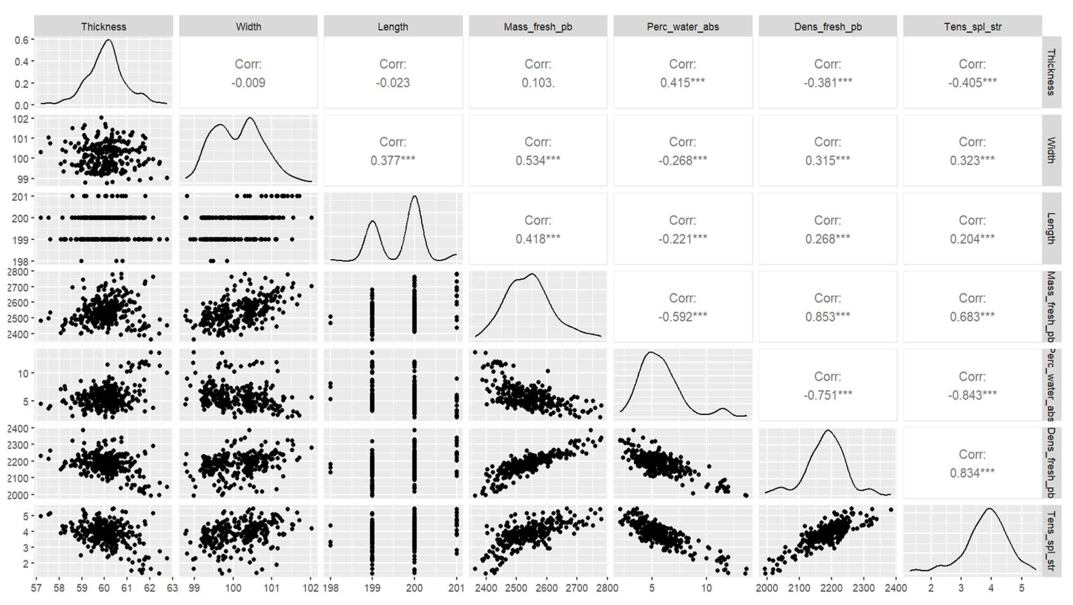
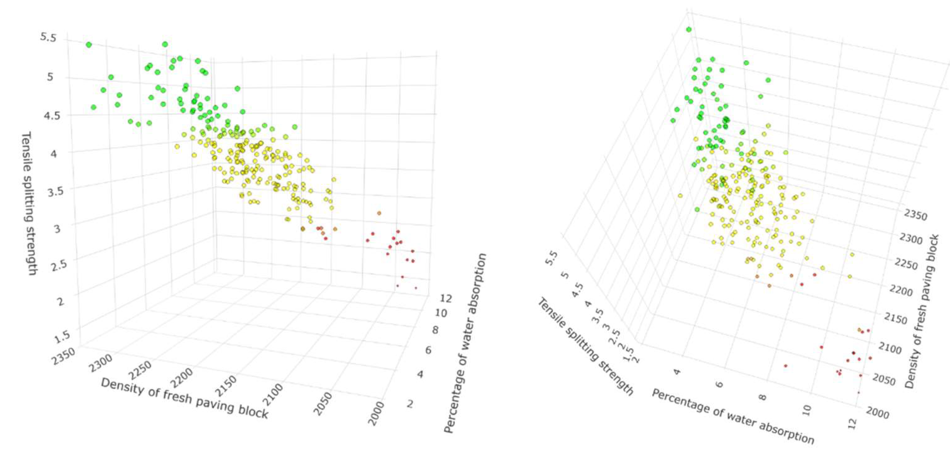
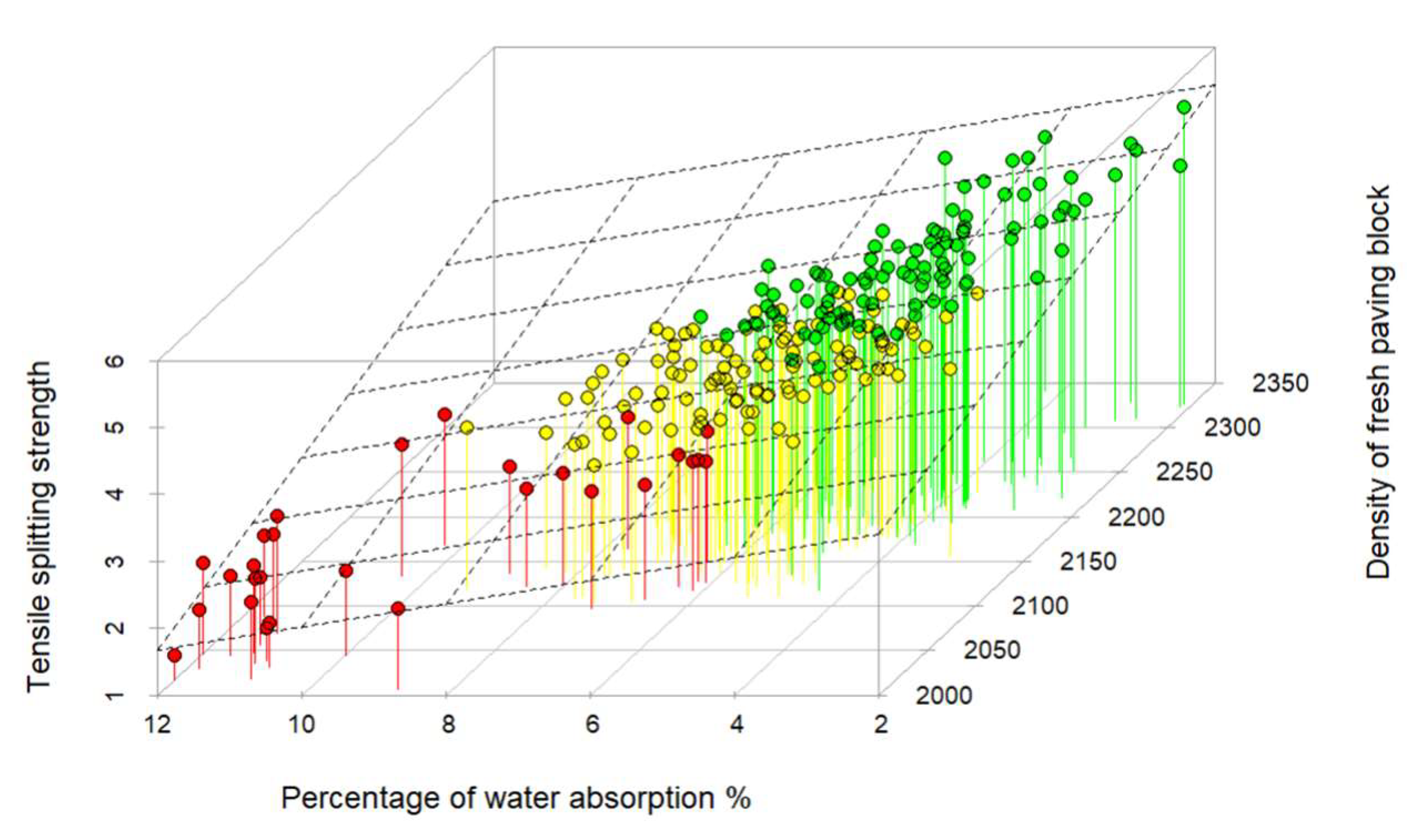
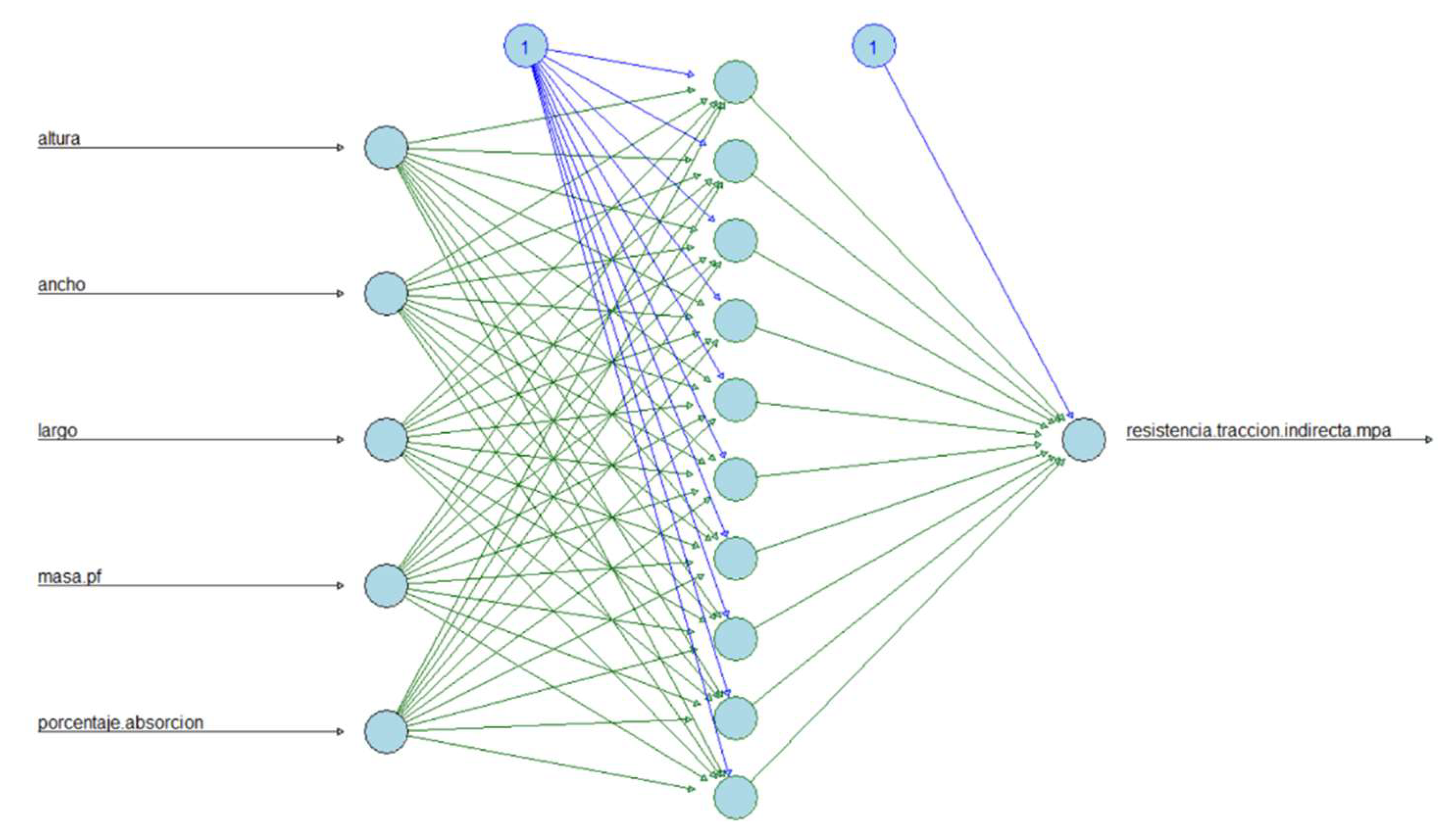
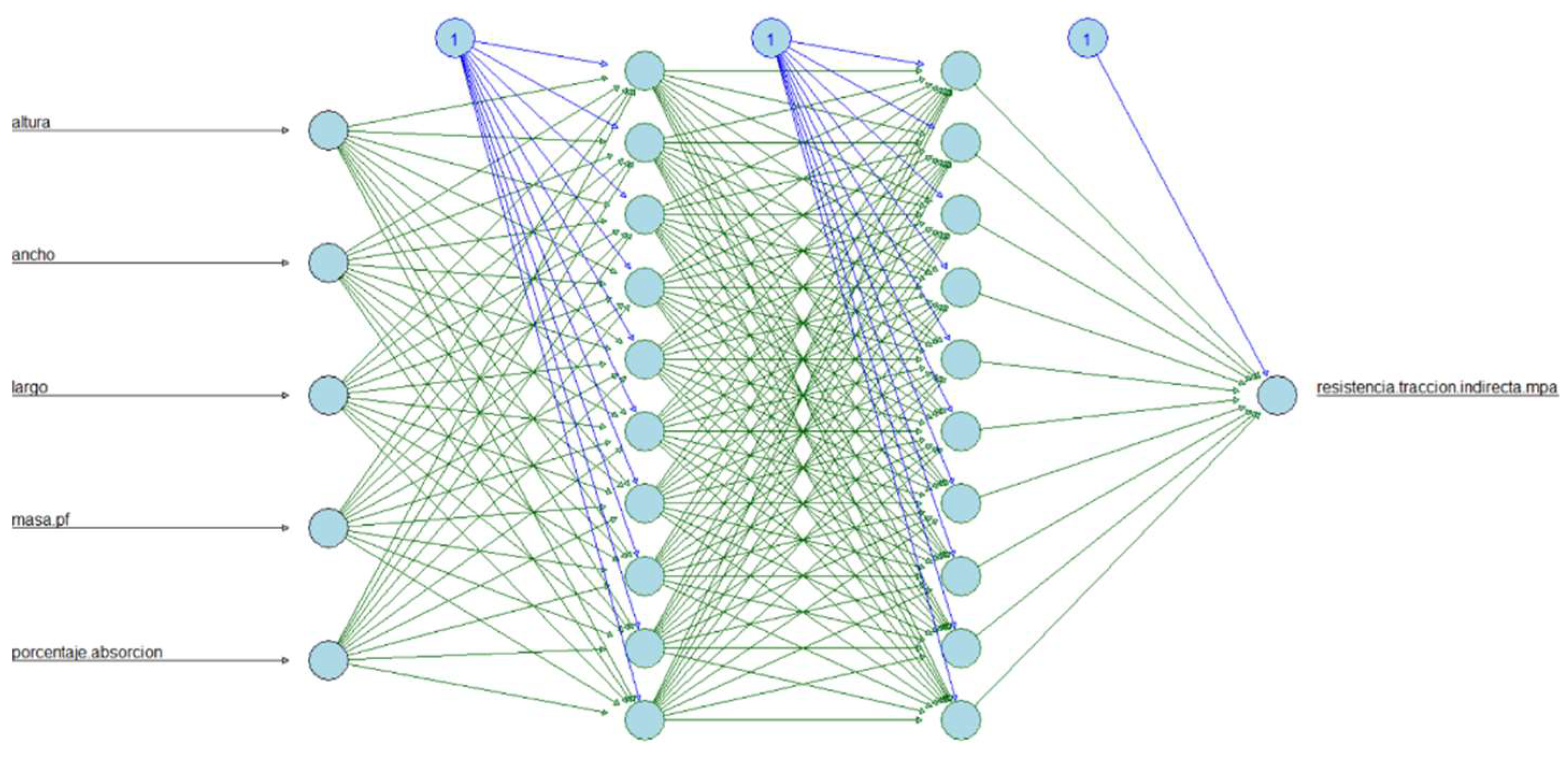
The variables that enter the models of multivariate techniques, also called input, predictor or independent, are: length mm, width mm, height mm, the mass of the fresh paving blocks (piece fresh from the vibro-compacting process) expressed in grams and the percentage of absorption based on the NTE INEN 3040 standard. Additionally, since the dimensional variables of the paving blocks and the mass of the fresh product can be reformulated into a new variable called the density of the fresh product expressed in units of (kg/m³), it was taken into account this variable together with the percentage of water absorption to make the prediction and compare the multivariate methods.

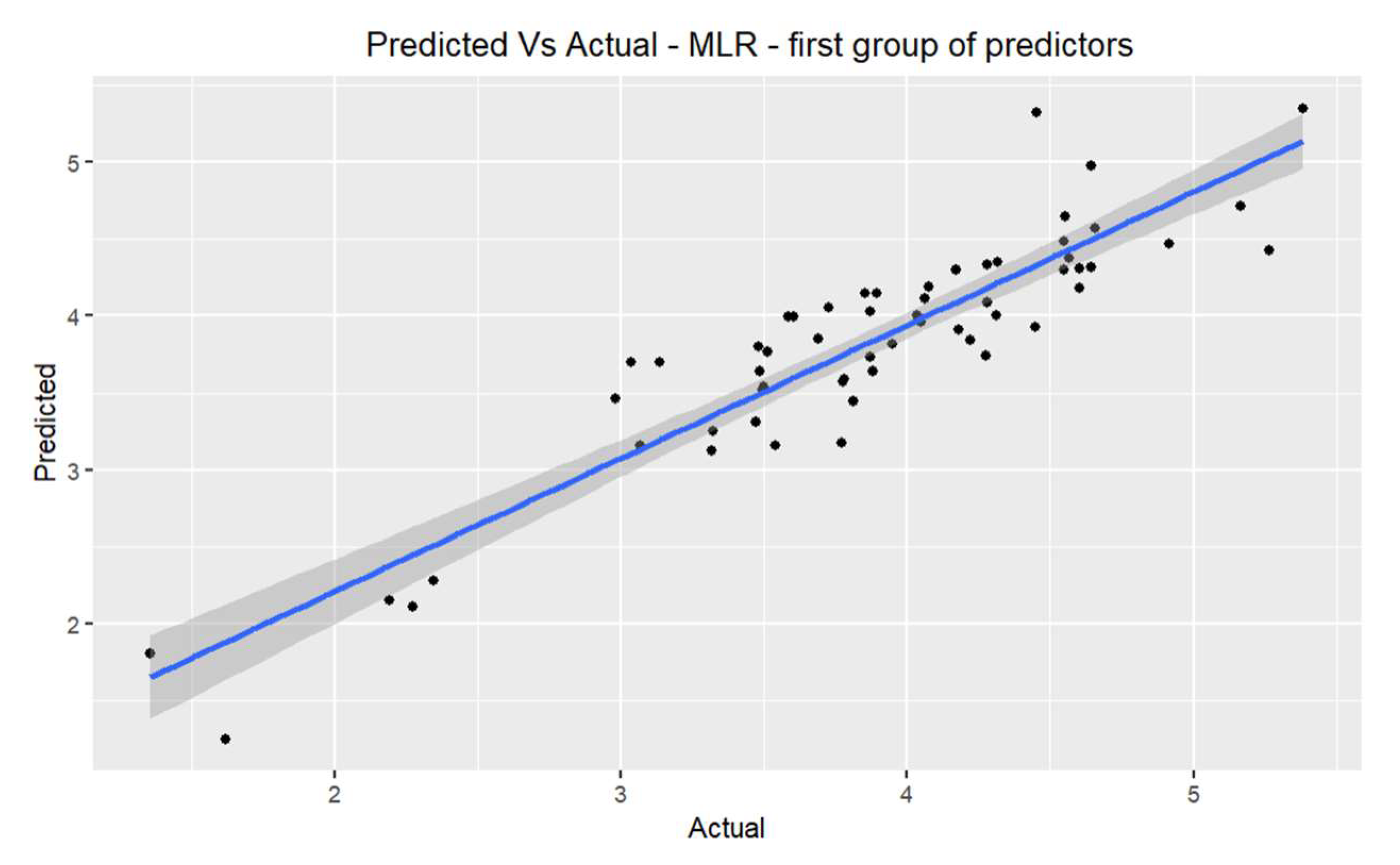
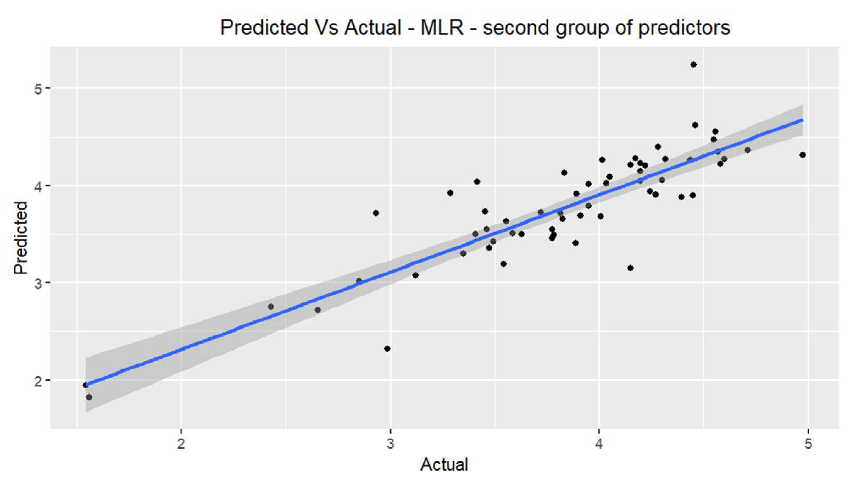
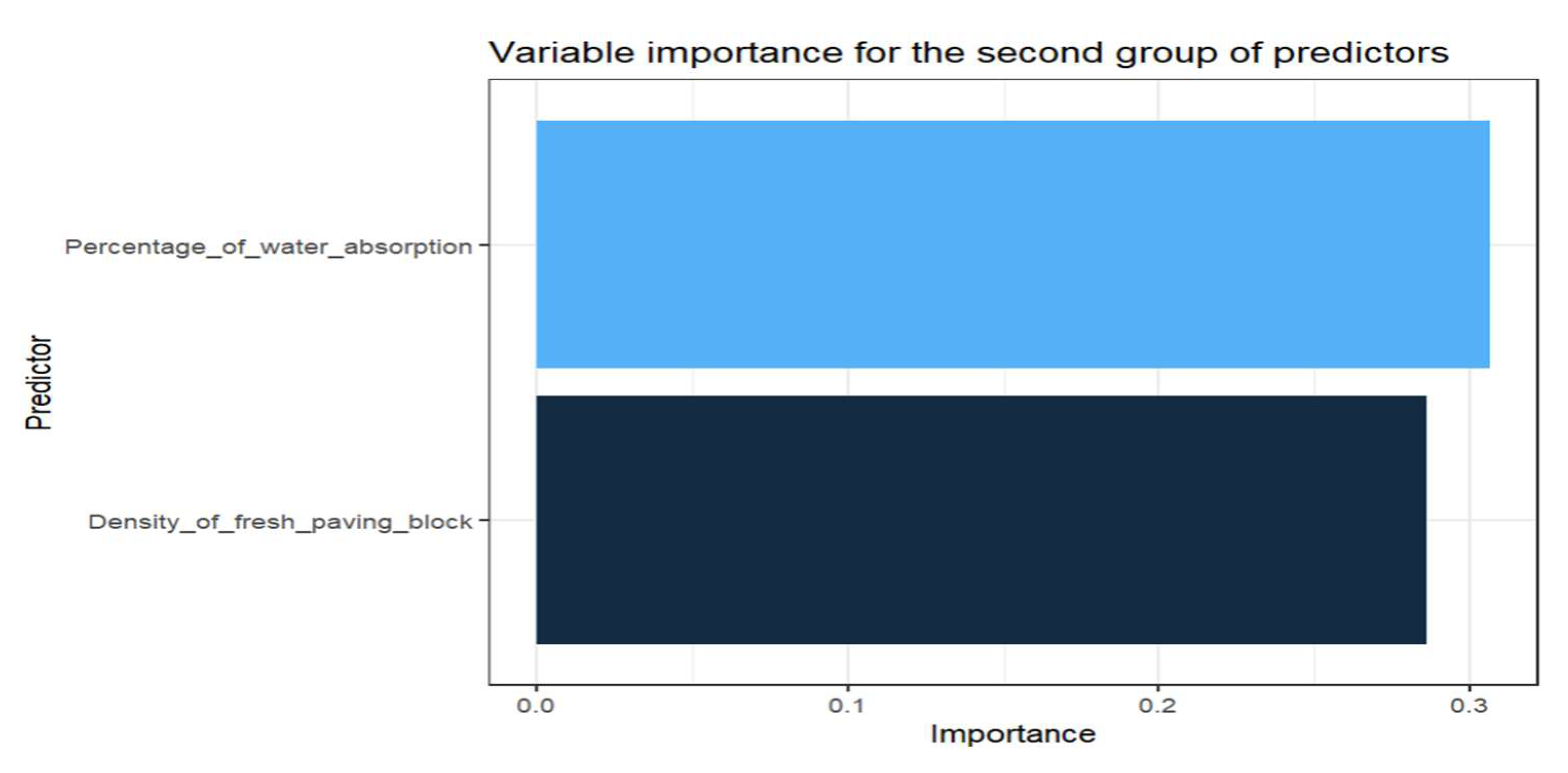
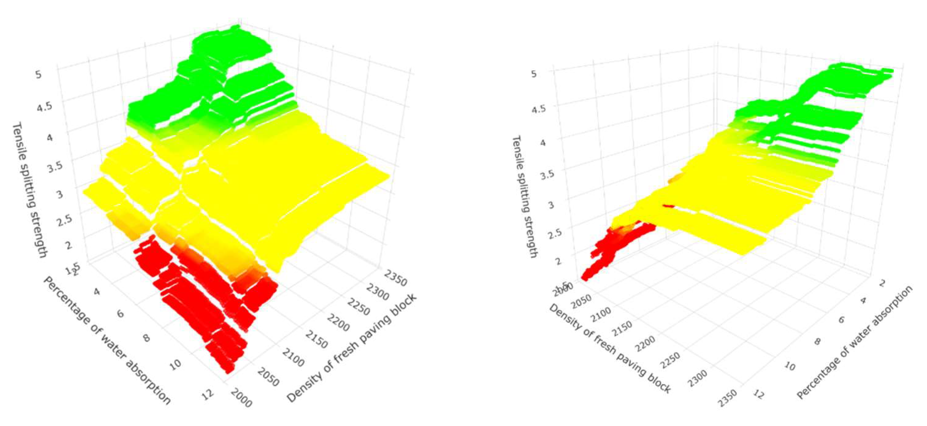
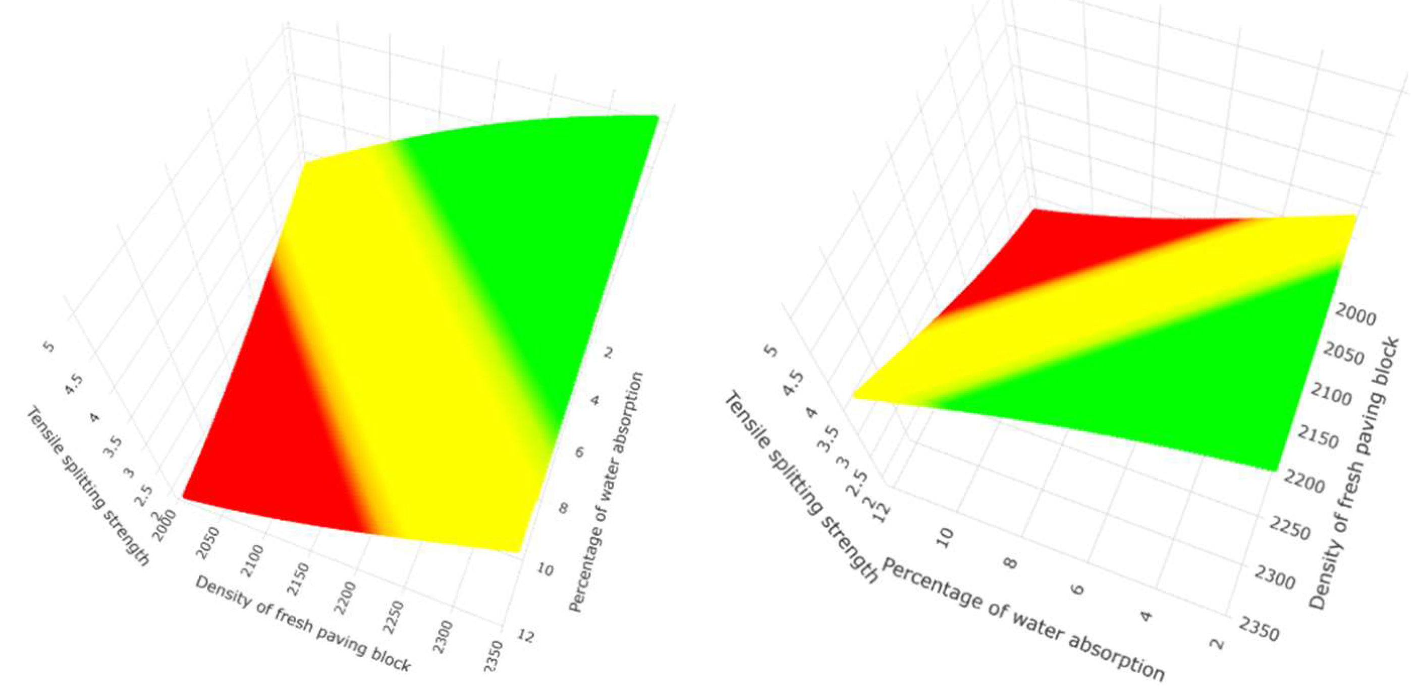
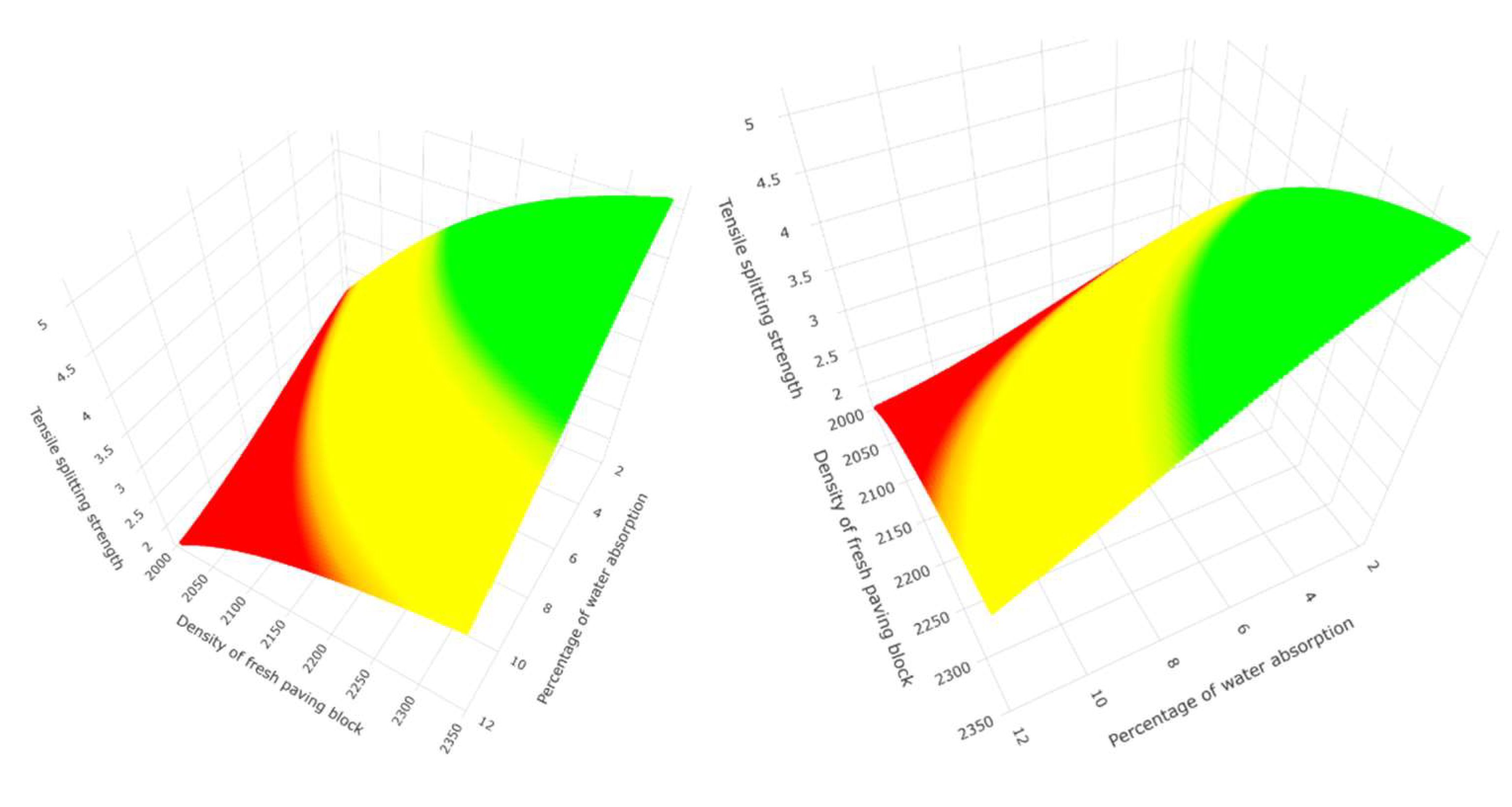
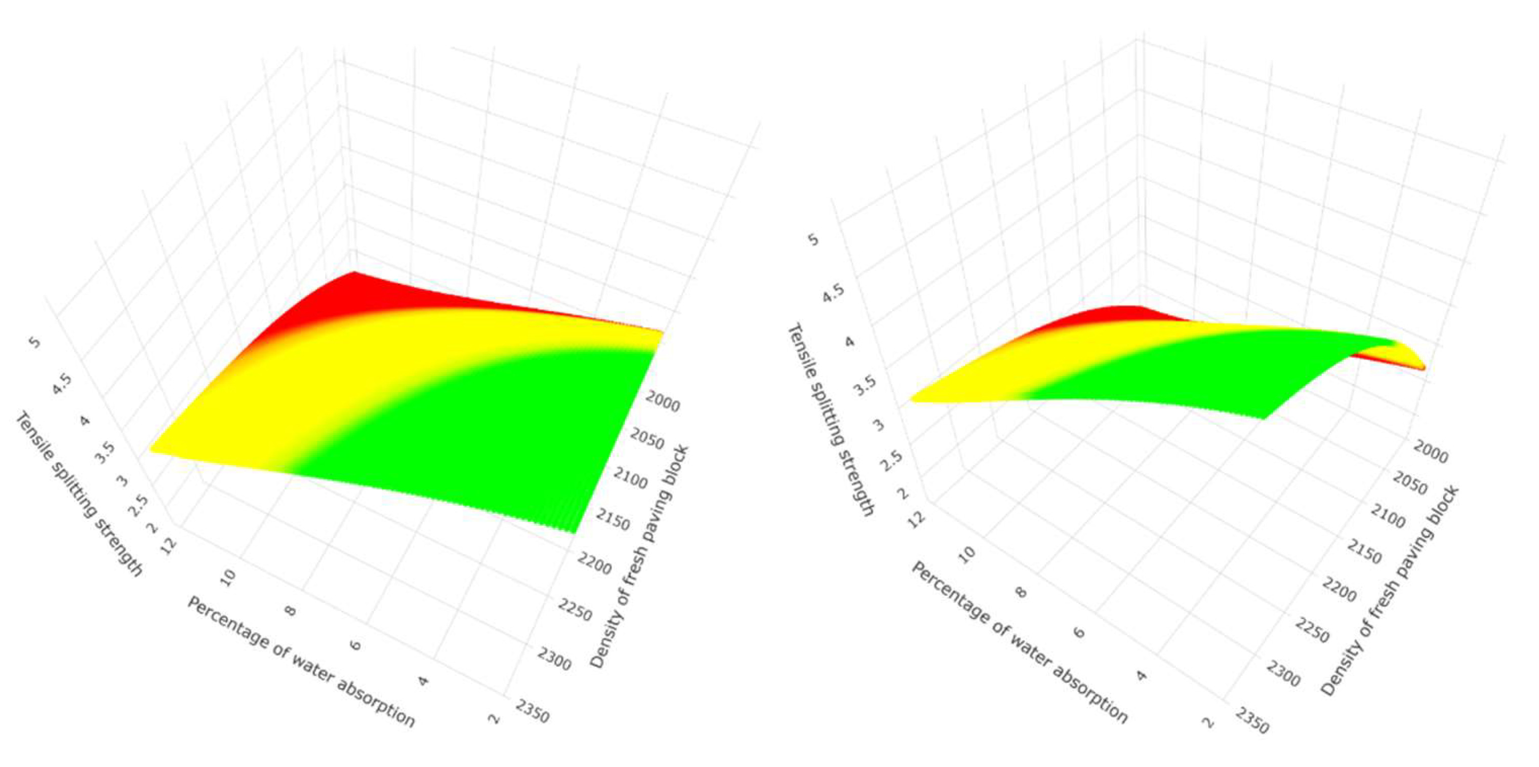
The response variable, also called dependent or output, is the indirect tensile strength in megapascals (MPa), which will depend on the predictor variables, which are grouped into: First group of predictor variables (5): Length, width, thickness, mass of the fresh product and absorption water percentage. The second group of predictor variables (2): Density of the fresh paving block and percentage of water absorption.

Water absorption. The water absorption test is carried out by reference to the NTE INEN 3040 (2016) standard, which indicates that to determine the absorption rate, the paving block must be submerged in potable water at 20 ±5 ^o C minimum for three days and then clean the surface excess water with a moistened cloth, weigh the moistened paving block to a constant mass. In the same way, an oven is used to find the mass of the dry paving block, and it is placed for a minimum period of 3 days at 105 ±5 ^o C until constant mass. The calculation is made by the difference between the saturated and dry mass divided by the dry mass. This would correspond to the percentage of the maximum mass of water that the paving block has absorbed from the dry state to the saturated state. The calculation formula is as follows:

W_{a} = \frac{M_{1} - M_{2}}{M_{2}}

(1)

M_{1}

is the mass of the specimen saturated with water, expressed in grams.

M_{2}

is the final mass of the dry specimen, expressed in grams.

Fresh paving block weight (mass). It is the mass of the paving block expressed in grams taken just after it leaves the mould in the vibro-compaction process.

Thickness (height), length and width of the paving block. The height of the paving block, or thickness, is the distance between the lower and upper face. In practice, the height variation is given by the vertical mobility of the mechanical parts in the vibro-compacting, where the plate of tamping compresses the mixture into the mould. The width and length of the paving blocks are taken from one end to the other.

Tensile splitting strength. The tensile splitting strength test is carried out using a hydraulic press, giving the measured load at failure in newtons, and the strength is calculated by applying the following formula indicated in the standard NTE INEN 3040 (2016) :

T = 0,637 * k * \frac{P}{S}

(2)

Where T is the paving block strength in MPa, P is the measured load at failure in Newtons, and S is the area of failure plane in mm² that results from the multiplication of the measured failure length and the thickness at the failure plane of the paving block, and k=0.87 for a thickness of 60 mm.

Mahalanobis Distance. The importance of identifying outlier data in a database is that these can distort the statistical analysis, and therefore the distance to the centroid and the shape are taken into account; the Mahalanobis distance takes these two premises into account [23]. The study by [24] indicates that in the multivariate field with Gaussian data, the Mahalanobis distance follows a chi-square distribution, where p means degrees of freedom and represents the number of variables. The Mahalanobis distance measures the amount of the standard deviation of an observation or individual from the mean of a distribution, considering correlations for multivariate analysis. The Mahalanobis distance transforms to a Euclidean distance when covariance matrix is the identity matrix [25]. A multivariate normal distribution is defined as:

f (X) = {(\frac{1}{2 π})}^{p / 2} * {|Σ|}^{- 1 / 2} * e x p \{- \frac{1}{2} {(x - μ)}^{T} Σ^{- 1} (x - μ)\}

(3)

Where

Σ

is the covariance matrix,

μ

the mean vector, if X is a vector with p variables, which follows a multivariate normal distribution

X ~ N_{p} (μ, Σ

), then the mahalanobis distance square

D^{2}

follows a chi-squared distribution with p degrees of freedom

D^{2} ~ X_{p}^{2}

. Mahalanobis represents the distance between each data point and its centre of mass and is defined by the following formula:

D^{2} = {(X - μ)}^{T} Σ^{- 1} (X - μ)

(4)

Simple linear regression. Simple linear regression allows one to relate two variables: variable Y, called response or dependent, and variable X, predictor or explanatory. The regression of the two random variables is given by the expected value of Y when X takes a specific value (X=x). If we consider linear regression with intercept

β_{0}

, slope

β_{1}

e_{i}

that represents the random error of

Y_{i}

, [26] explains that the residuals

\hat{e_{i}}

are

y_{i} - {\hat{y}}_{i}

where

{\hat{y}}_{i}

is the fitted value of y.

Y_{i} = E (Y| X = x) + e_{i} = β_{0} + β_{1} x + e_{i}

(5)

The popular method for obtaining

β_{1}

β_{0}

is RSS ordinary least squares to minimize the difference between the observed and predicted values. The minimization is done by differentiating RSS concerning the coefficients

b_{0}

and

b_{1}

and setting it equal to 0.

R S S = \sum_{i = 1}^{n} {\hat{e}}_{i}^{2} = \sum_{i = 1}^{n} {(y_{i} - b_{0} + b_{1} x_{i})}^{2}

(6)

The structural assumptions of the regression model are the linearity that explains that Y depends on x through linear regression, the homoscedasticity indicates that the variance of the errors when X=x must be common, better explained as

V a r (e| X = x) = σ^{2}

, the normality assumption indicates that the errors must follow a normal distribution with 0 mean and variance

σ^{2}

and finally the independence of the errors. The inference of the linear regression under the previous assumptions

{\hat{β}}_{1}

follows a normal distribution with mean

β_{1}

and variance

(σ^{2} / S X X)

where

S X X = \sum_{i = 1}^{n} {(x_{i} - \bar{x})}^{2}

; if we consider

σ^{2}

unknown, then the test statistic follows a distribution of T-student with n-2 degrees of freedom, where

H_{o}

β_{1} = 0

is the null hypothesis and

H_{a}

β_{1} \neq 0

is the alternative hypothesis. T is described by the expression:

T = \frac{{\hat{β}}_{1} - β_{1}}{s / \sqrt{S X X}} ~ t_{n - 2}

(7)

Similarly, for

β_{0}

, the T statistic follows a T-student distribution with n-2 degrees of freedom, where the null hypothesis is

H_{o}

β_{0} = 0

and the alternative hypothesis is

H_{a}

β_{0} \neq 0

T = \frac{{\hat{β}}_{0} - β_{0}}{s / \sqrt{\frac{1}{n} + \frac{{\bar{x}}^{2}}{S X X}}} ~ t_{n - 2}

(8)

The analysis of variance allows decomposing the variability by analyzing the mean of Y, the predicted and observed points; the total variability is separated into the sum of the variability explained by the model plus the unexplained variability or error. The total sum of squares is SST = SYY =

\sum_{i}^{n} {(y_{i} - \bar{y})}^{2} a n d S S T = S S r e g +

R S S

, where

S S r e g

is the sum of squares of the regression (

S S r e g)

\sum_{i}^{n} {({\hat{y}}_{i} - \bar{y})}^{2}

and

R S S

is the sum of squares of the residuals

R S S

\sum_{i}^{n} {(y_{i} - {\hat{y}}_{i})}^{2}

y_{i} - \bar{y} = (y_{i} - {\hat{y}}_{i}) + ({\hat{y}}_{i} - \bar{y})

(9)

S S T = S S r e g + R S S

(10)

The F statistic follows an F distribution with 1 and n-2 degrees of freedom, where the null hypothesis is

H_{o}

β_{1} = 0

and the alternative hypothesis is

H_{a} : β_{1} \neq 0

. It can be seen that if the null hypothesis is rejected, then Y depends on X.

F = \frac{S S r e g / 1}{\frac{R S S}{(n - 2)}} ~ F_{1, n - 2}

(11)

The coefficient of determination in linear regression is given by:

R^{2} = \frac{S S r e g}{S S T}

(12)

Multiple Linear Regression (MLR). According to [26], the response variable (Y) in MLR is predicted and related to multiple explanatory or predictor variables, where the expectation of Y when each variable X takes a specific value is represented as:

E (Y| X_{1} = x_{1}, X_{2} = x_{2}, . ., X_{p} = x_{p}) = β_{0} + β_{1} x_{1} + \dots + β_{p} x_{p}

(13)

Y_{i} = β_{0} + β_{1} x_{1 i} + \dots + β_{p} x_{p i} + e_{i}

(14)

The sum of squares for the multivariate case is:

R S S = \sum_{i = 1}^{n} {\hat{e}}_{i}^{2} = \sum_{i = 1}^{n} {(y_{i} - {\hat{y}}_{i})}^{2} = \sum_{i = 1}^{n} {(y_{i} - b_{0} + b_{1} x_{1 i} + \dots + b_{p} x_{p i})}^{2}

(15)

Multiple linear regression is denoted as:

Y = X β + e

(16)

Each term expressed in vectors and matrices indicates the following:

Y = (\begin{matrix} y_{1} \\ \begin{matrix} y_{2} \\ ⋮ \end{matrix} \\ y_{n} \end{matrix}), X = (\begin{matrix} \begin{matrix} \begin{matrix} 1 & x_{11} & \dots \end{matrix} \\ \begin{matrix} \begin{matrix} 1 & x_{21} & \dots \end{matrix} \\ \begin{matrix} \begin{matrix} ⋮ & ⋮ & ⋮ \end{matrix} \\ \begin{matrix} 1 & x_{n 1} & \dots \end{matrix} \end{matrix} \end{matrix} \end{matrix} & \begin{matrix} x_{1 p} \\ x_{2 p} \\ \begin{matrix} ⋮ \\ x_{n p} \end{matrix} \end{matrix} \end{matrix}), β = (\begin{matrix} β_{1} \\ \begin{matrix} β_{2} \\ ⋮ \end{matrix} \\ β_{p} \end{matrix}), e = (\begin{matrix} e_{1} \\ \begin{matrix} e_{2} \\ ⋮ \end{matrix} \\ e_{p} \end{matrix})

The estimated coefficients of each term can be calculated by linear algebra calculus, where the term

X {(X^{T} X)}^{- 1} X^{T}

is defined as Hat Matrix (H) and the residual maker matrix as M, which is equal to

I_{n} - H

where

I_{n}

is the identity matrix, the projection

\hat{Y}

is equal a

H * Y

so in the regression hyperplane,

\hat{Y}

is a transformation of Y.

\hat{β} = {(X^{T} X)}^{- 1} X^{T} Y

(17)

If the errors follow normal distribution with constant variance, then the T statistic follows a student’s t distribution with n-p-1 degrees of freedom and is given by:

T_{i} = \frac{{\hat{β}}_{i} - β_{i}}{s e ({\hat{β}}_{i})} ~ t_{n - p - 1}

(18)

The term

s e (\hat{β})

is the estimated standard deviation of

{\hat{β}}_{i}

where the null hypothesis indicates that

H_{o}

β_{i} = 0

and the alternative hypothesis is

H_{a}

β_{i} \neq 0

. In the analysis of variance in the multivariate case, as in the case of simple linear regression, the total variability is equal to the variability explained by the model plus the unexplained variability or error. The F statistic follows an F distribution with p and n-p-1 degrees of freedom where the null hypothesis is Ho:

β_{1} = β_{2} = β_{3} = \dots = β_{p} = 0

and the alternative hypothesis indicates that

H_{a}

a t l e a s t s o m e o f t h e β_{i} \neq 0

F = \frac{S S r e g / p}{\frac{R S S}{(n - p - 1)}} ~ F_{p, n - p - 1}

(19)

Adding the number of predictors increases

R^{2}

, so

R_{a d j}^{2}

is used.

R_{a d j}^{2} = 1 - \frac{R S S / (n - p - 1)}{S S T / (n - p)}

(20)

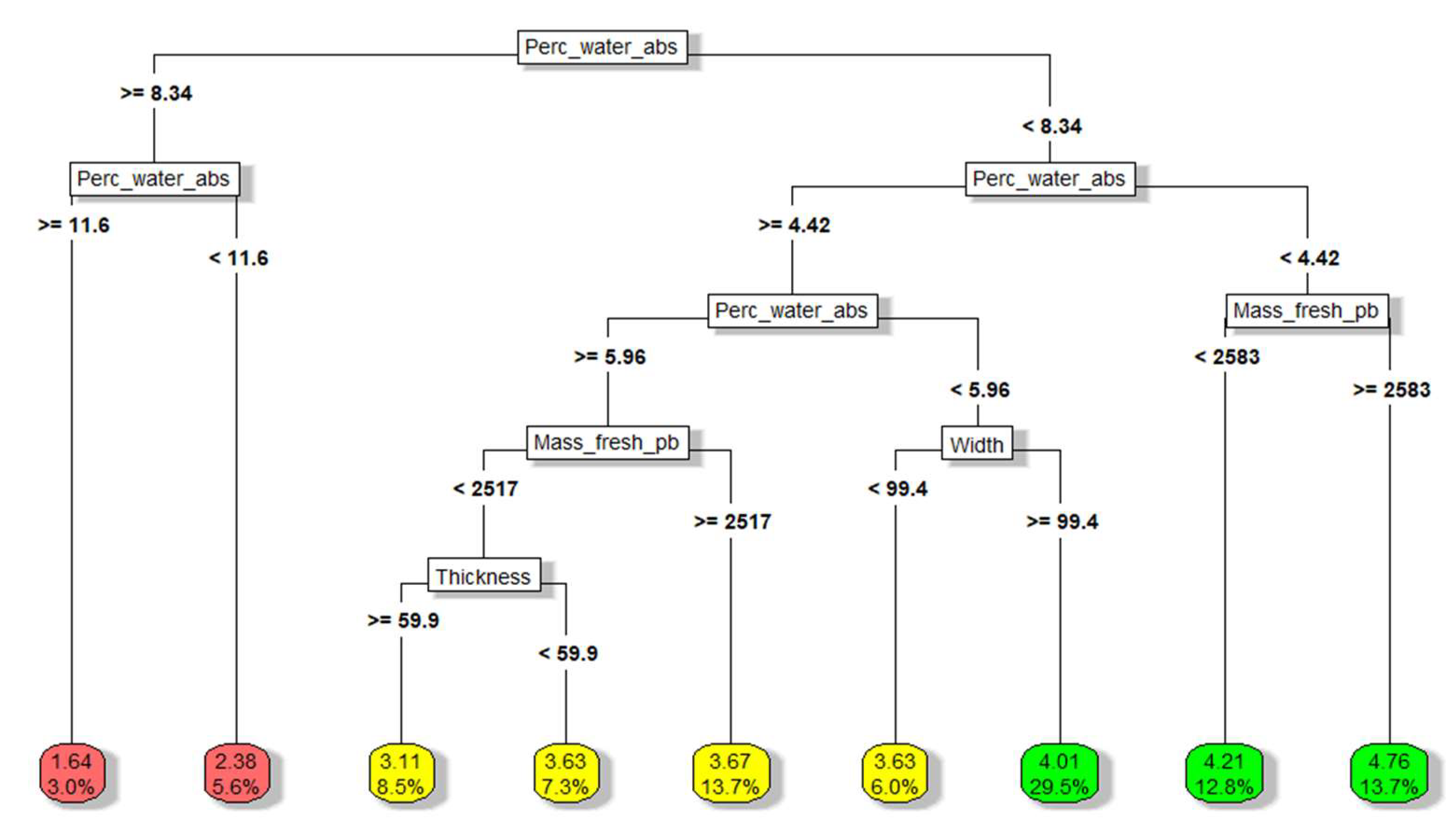
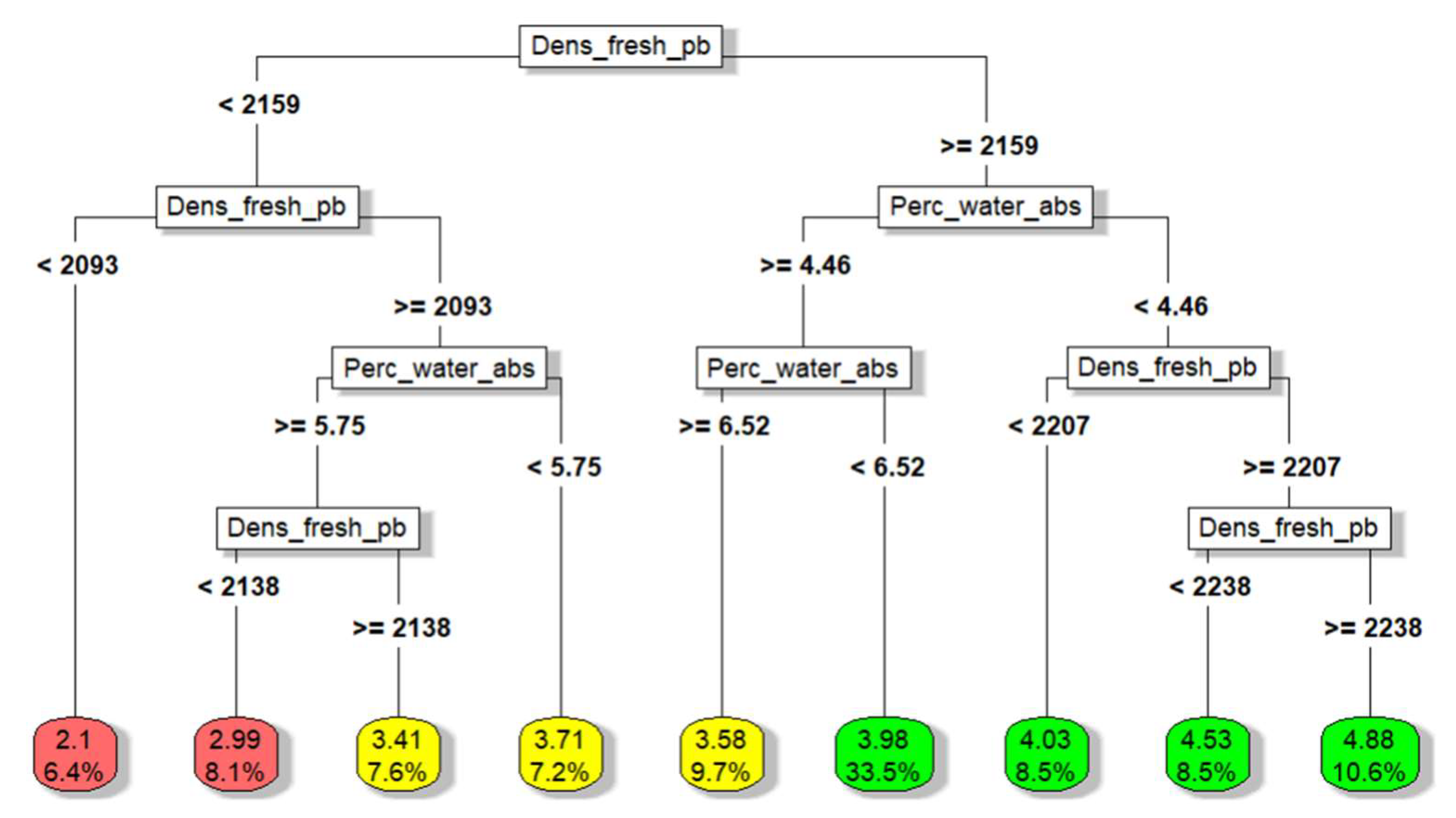
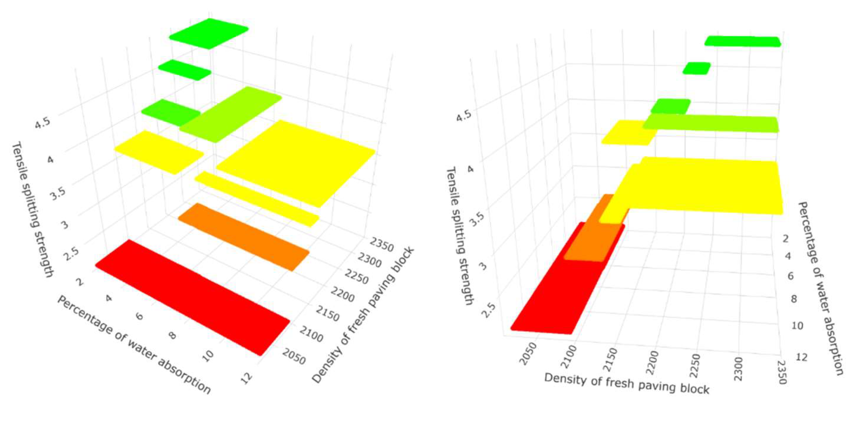
Regression trees. A decision tree is an algorithm in machine learning that can be used in regression and classification; that is a white box where they are intuitive and easy to interpret. For the regression case, the tree, instead of predicting a class, predicts a value that is the average value across the training instances of the node. Instead of minimizing impurity, the regression tree minimizes the mean squared error MSE [27]. The cost function for regression is:

J (k, t_{k}) = \frac{m_{l e f t}}{m} {M S E}_{l e f t} + \frac{m_{r i g h t}}{m} {M S E}_{r i g h t}

(21)

Where m is the number of instances to the left or right, MSE is the mean square error.

M S E = \sum_{i ϵ n o d e} {({\hat{y}}_{n o d e} - y^{(i)})}^{2}

(22)

{\hat{y}}_{n o d e} = \frac{1}{m_{n o d e}} \sum_{i ϵ n o d e} y^{(i)}

(23)

The limits on the decision trees are perpendicular to the axis (orthogonal) and are sensitive to variations in training. The regression trees, according to [28], generate divisions of the database into more homogeneous groups, with a set of “if” and “then” conditions being easily interpretable with different predictors. A disadvantage that could occur is instability with minor changes in the data. The oldest and most widely used technique is CART by [29], whose methodology is to find the predictor and the dividing value of the base whose squared error is the smallest.

S S E = \sum_{i ϵ S 1} {(y_{i} - {\bar{y}}_{1})}^{2} + \sum_{i ϵ S 2} {(y_{i} - {\bar{y}}_{2})}^{2}

(24)

{\bar{y}}_{1}

represents the subgroup mean

S_{1}

{\bar{y}}_{2}

represents the subgroup mean

S_{2}

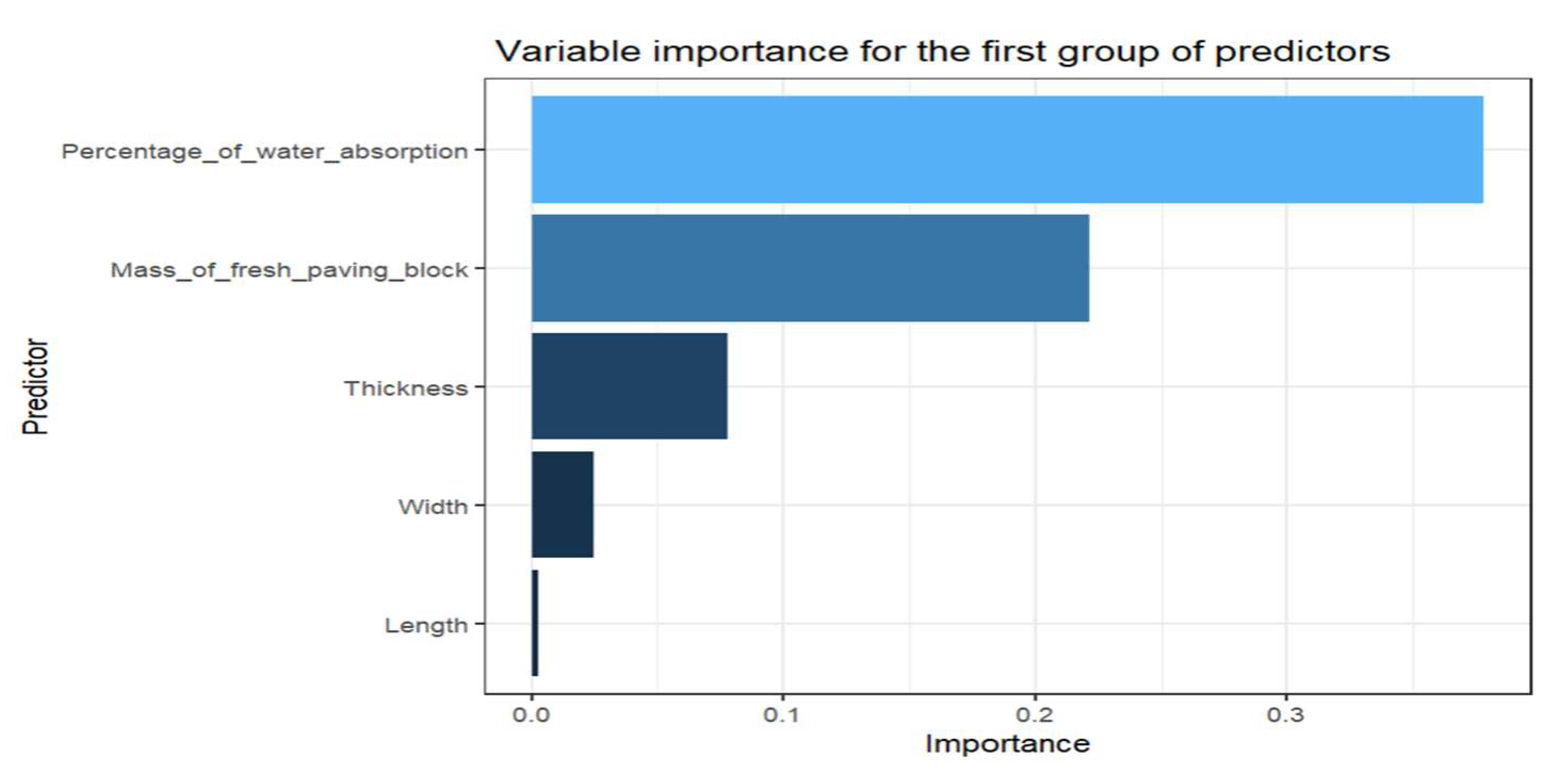
, the division process continues within the sets

S_{1}

and

S_{2}

up to a stopping criterion. The predictor’s relative importance can be calculated using SSE, where the predictors higher up the tree or more frequent are the most important.

Random forests. In the research by [30], an algorithm called the random forest allows for predicting and reducing overfitting. The procedure consists of choosing the number of tree models to be built from 1 to m, obtaining an initial sample, and then training the tree model for each division; the predictors are randomly selected, the best one is chosen, and finally, the stopping criteria are used. Each tree model generates a prediction, and the m predictions are averaged to generate the final prediction. By randomly choosing the k variables in each division, their correlation decreases. Random forests are computationally more efficient tree by tree, and the predictors’ importance can also be seen through the permutation or impurity methodology. According to [28], the tree bagging procedure reduces the prediction variance. The ensemble method is the algorithm that analyzes the predictions as a whole, obtaining the predictions of each individual tree with different random subsets. [27]. Analyzing the predictions together will yield better results than just one prediction. Random forests are trained by bagging with max_samples.

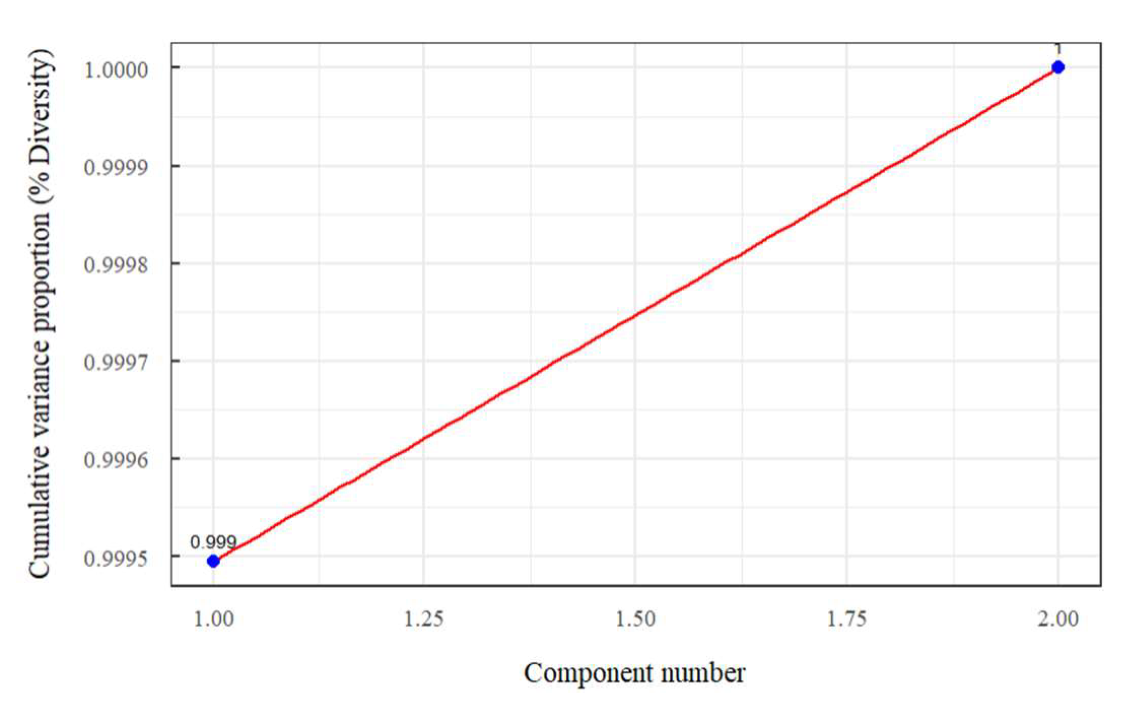
Principal component analysis. It is a dimension reduction technique that occupies the orthogonal transformation so that a group of correlated n-dimensional variables can maintain their variability information in other uncorrelated k-dimensional ones. The general process consists first of data standardisation so that the base has a mean of zero and a variance of one. The covariance matrix, correlation matrix, eigenvectors and eigenvalues are calculated. The first eigenvectors representing the most significant variability are chosen [31]. Research carried out by [32] indicates that this technique was developed by Karl Pearson and Harold Hotelling independently. The technique linearly transforms multivariate data into a new uncorrelated set of variables. The eigenvectors are vectors that do not change position when a data transformation occurs and represent the axis of maximum variance called the principal component.

According to [33], Principal components are commonly defined as the matrix multiplication between the eigenvectors of the correlation matrix (A) and the standardized variables (

X^{*}

z = A^{T} X^{*}

(25)

The principal components calculated by covariance have a drawback, and it is the sensitivity to the units of measurement, for which it is done using the correlation matrix with the standardized variables since each variable has a different unit of measurement. Also, the sizes of the variances of the principal components have the same implications in correlation matrices as in covariance matrices. One of the properties of the principal components using the correlation matrix is that they do not depend on the absolute values of the correlation.

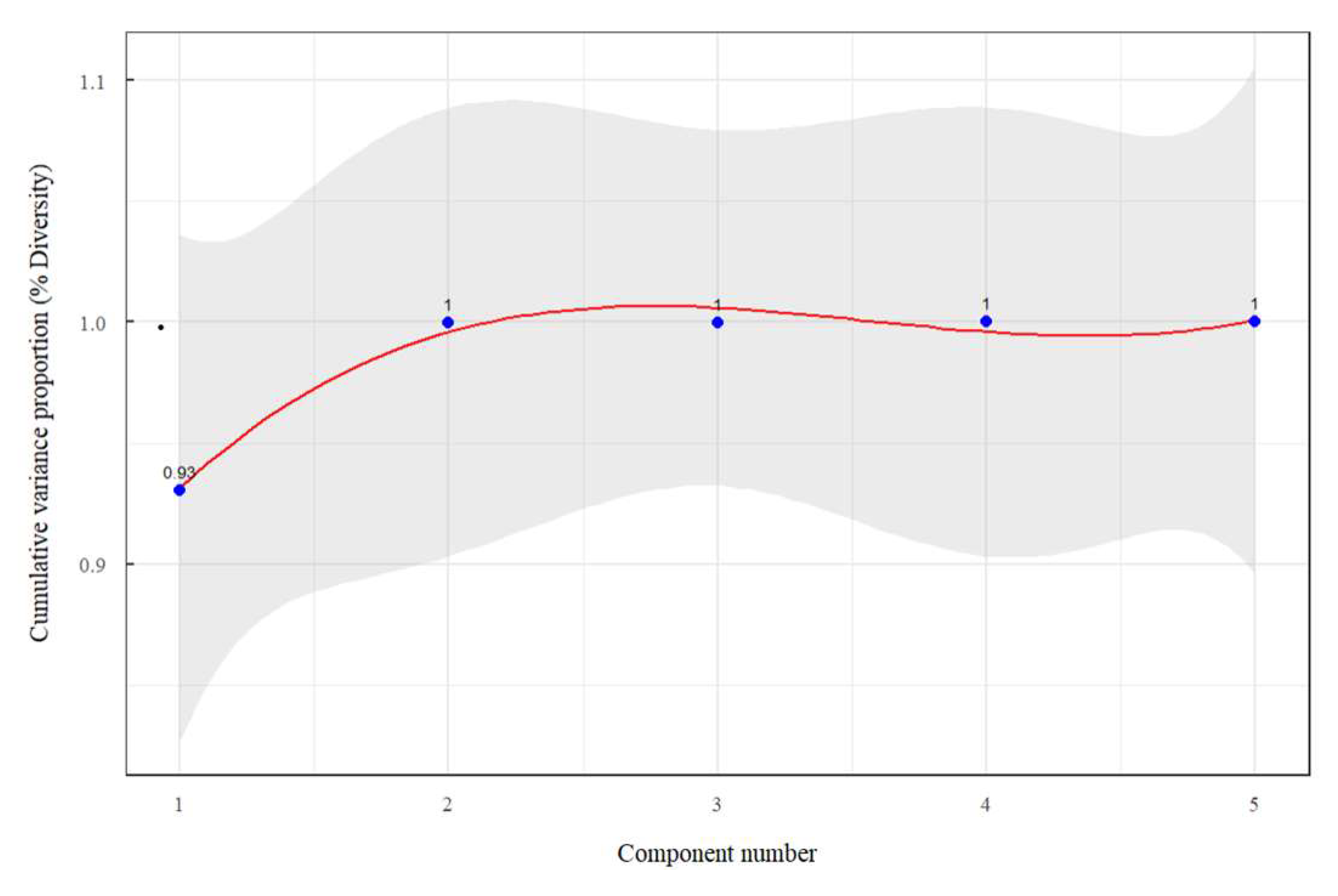
According to studies, [34] principal component analysis can determine the number of hidden layers in artificial neural networks, which represents sufficient variability for statistical analysis. On the other hand, the study by [35] lets to know the number of hidden layers in neural networks through principal component analysis to predict a continuous variable, giving good results through quality measures with optimal performance.

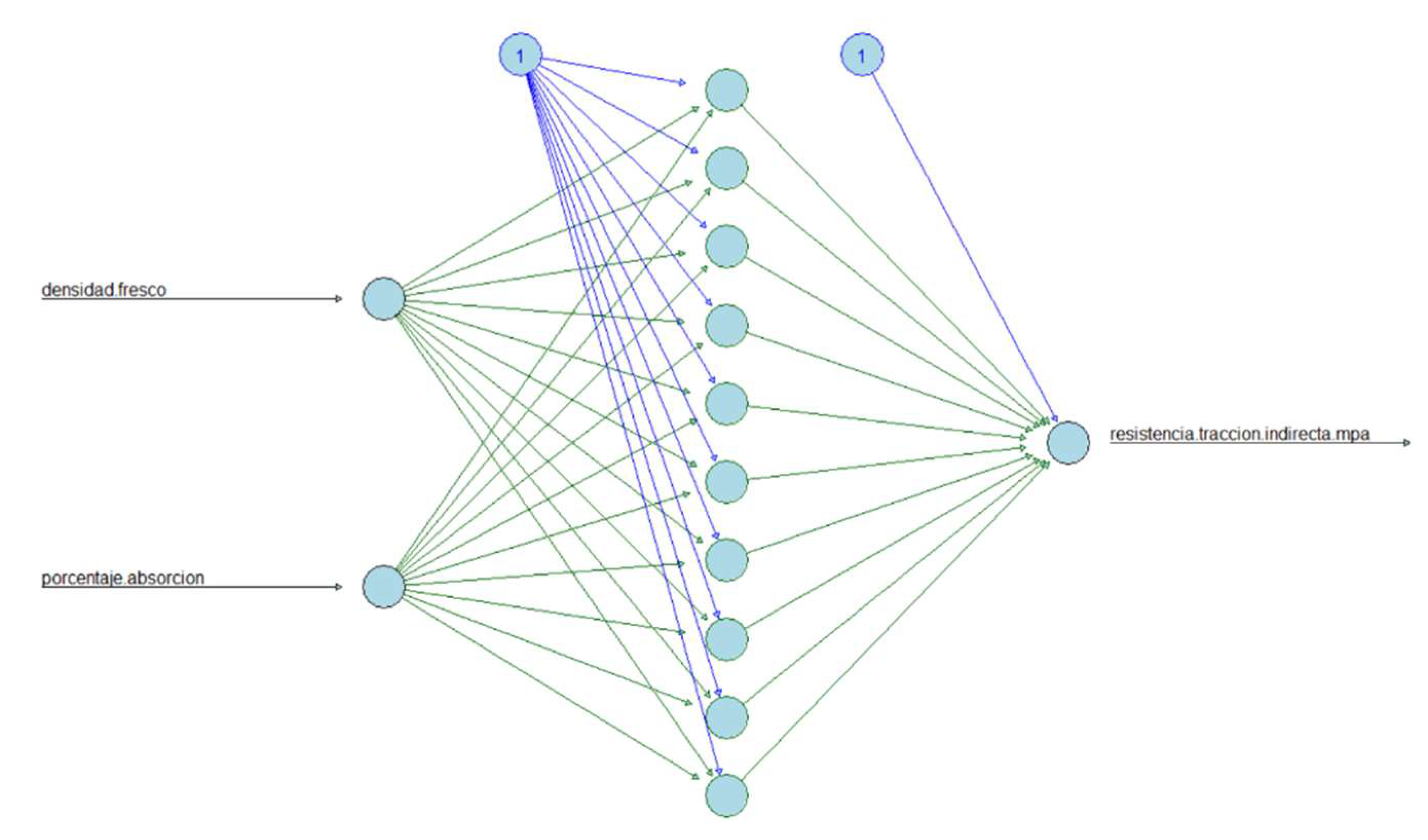
Artificial neural networks. Neural networks were inspired by the biological capacity of the brain, being so influential in machine learning to tackle tasks as complex as classifying millions of images, voice recognition, and beating world champions in mental sports. They were implemented in 1943 by McCulloch and Walter Pitts. In neural networks, the perceptron is a different neuron called threshold logic unit where the inputs are numbers just like the outputs, and each connection has a weight [27].

A fully connected layer has the following outputs

h_{W, b} (X)

, where X is the input matrix (instance rows and feature columns), W is the weight matrix (rows per input neurons and columns per artificial neuron), b is the polarization vector (connection weights of the bias neuron and the artificial neurons),

\emptyset

is the activation function.

h_{W, b} (X) = \emptyset (X W + b)

(26)

Learning has a rule: the perceptron connections are strengthened when the error is reduced, receiving one instance at a time and making the predictions. Perceptron learning is done by

{w_{i, j}}^{(n e x t s t e p)}

{w_{i, j}}^{(n e x t s t e p)} = w_{i, j} + η (y_{j} - {\hat{y}}_{j}) x_{i}

(27)

Where

w_{i, j}

is the weight of the connection between the input and output of the neurons,

x_{i}

is the input value of the instance,

{\hat{y}}_{j}

is the output value of the instance,

y_{j}

is the target output value, and

η

is the learning rate. The perceptron convergence theorem tells us that the algorithm converges to a solution if the instances are linearly separable. The multilayer perceptron, MLP, has an input layer (lower layer), hidden layers, and an output layer (upper layer).

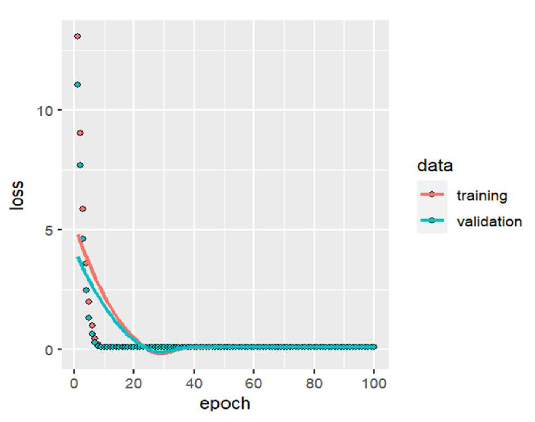
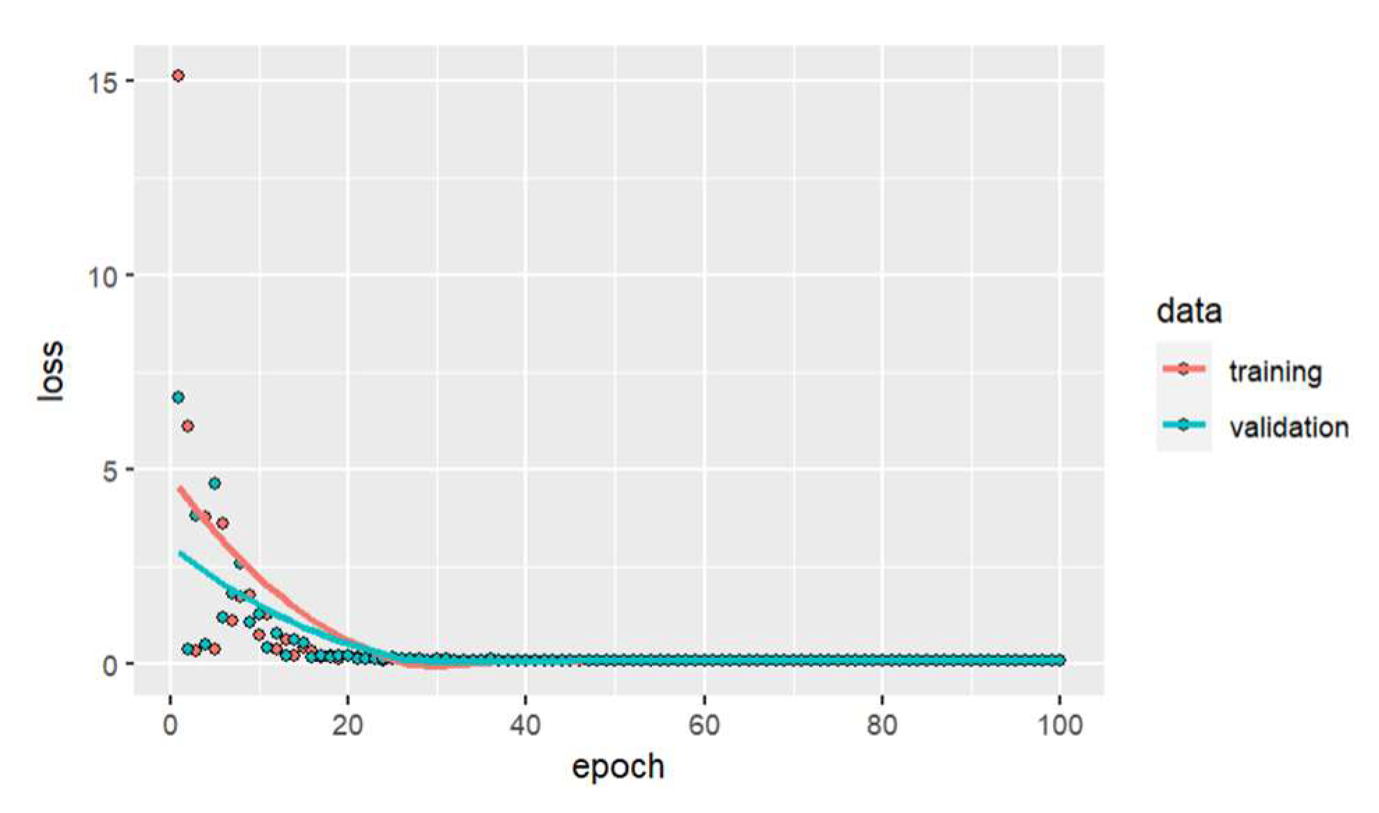
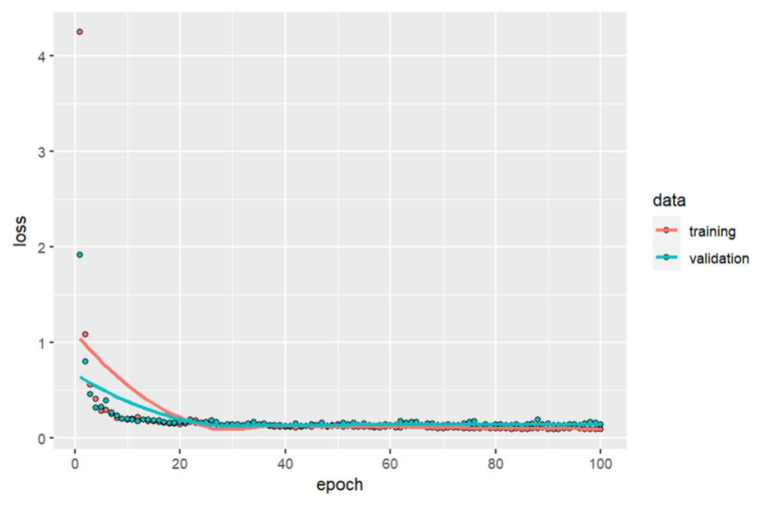
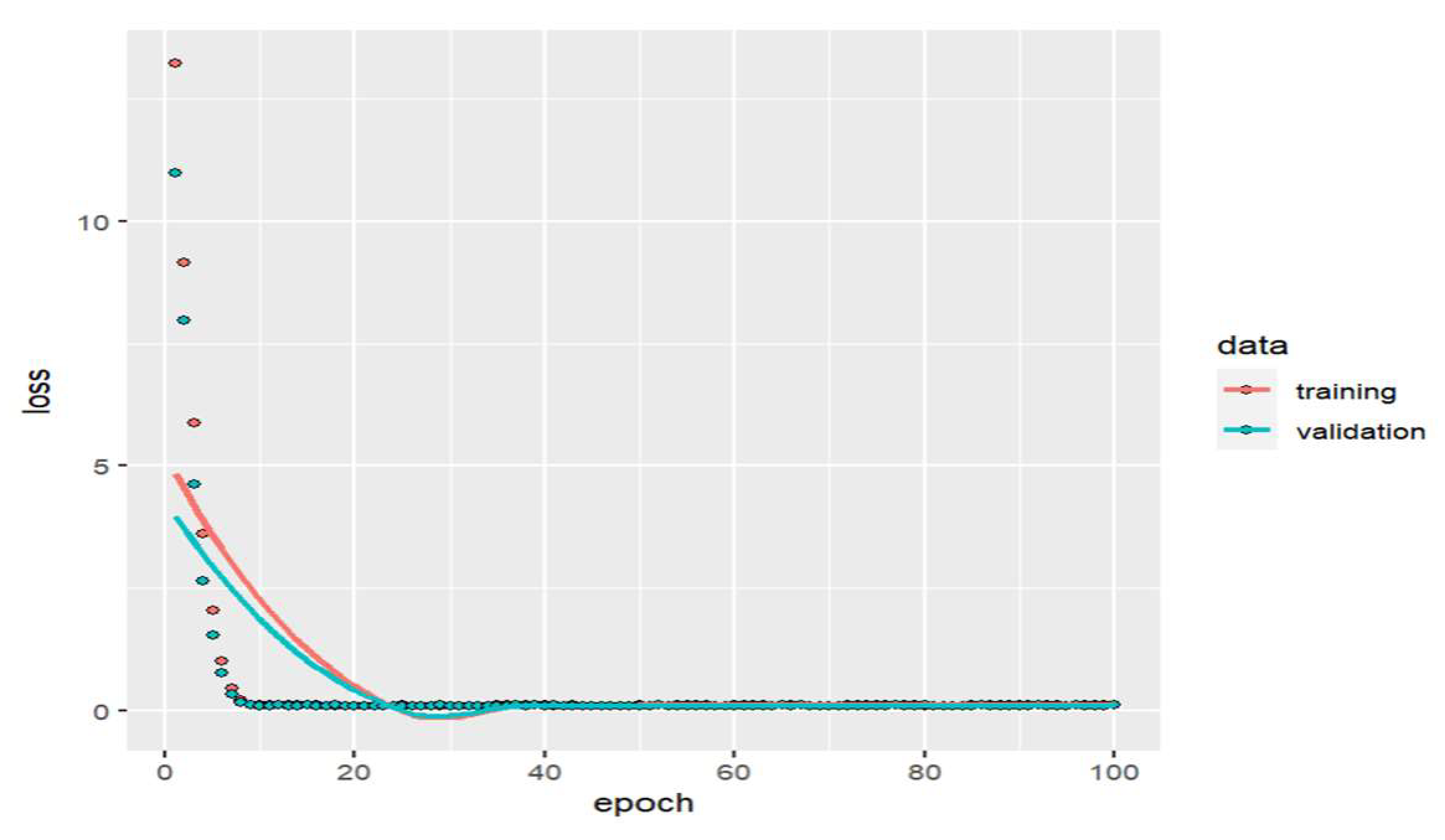
If the artificial neural network (ANN) has more than one hidden layer, it is called a DNN deep neural network. In 1986 in the article written by Rumelhart, Hinton and Williams, an algorithm called gradient descent was created to calculate the gradients automatically with one pass forward and another pass backwards; the process is repeated until converging to the solution. The procedure is to get a small group of instances and train it several times, creating an epoch. The small group goes through the input layer, hidden layers, and the output layer with a step forward, preserving the intermediate results and measuring the output error. The contribution of each connection to the error is calculated by applying the chain rule making it precise. It is returned to the input layer with the same rule, and the contribution to the connections’ error is measured; finally, the gradient descent is performed by adjusting the weights to reduce the error. If there is one output neuron, only one value will be predicted. According to [36], the sigmoid neuron has weights and a bias occupying the sigmoid function defined as

σ (z)

, where

z = w x + b

and the bias (b) is the introduced bias.

σ (z) = \frac{1}{1 + e^{- z}}

(28)

b = \frac{1}{1 + e^{- \sum_{j} w_{j} x_{j} - b}}

(29)

Considering the cost function to evaluate the model and quantify how well the objective is achieved, we have:

C (w, b) = \frac{1}{2 n} \sum_{x} {‖y (x) - a‖}^{2}

(30)

Where

w

represents the weights of the network, b are all the biases, n is the total training inputs, a is the vector of outputs when inputting an x, y(x) is the output desired, x sums over the training inputs, and C is the cost function. As the cost function approaches 0, as y(x) approaches the output a, gradient descent allows minimization of the cost function where it

∆ C

can be written as:

∆ C \approx \nabla C ∆ v

(31)

\nabla C

is the gradient vector and relates the changes of C to changing

v

, so

∆ v

is the vector of changes in position, and m is the number of variables.

\nabla C \equiv {(\frac{\partial C}{\partial v_{1}}, \dots, \frac{\partial C}{\partial v_{m}})}^{T}

(32)

Gradient descent repeatedly computes

\nabla C

looking like small steps in the direction C decreases the most. The backpropagation algorithm gives information on how to change the weights and biases in the behaviour of the neural network. The notation to use is l for the l-th layer , k is the k-th neuron of the l-th layer minus one ( l - 1 ), j is the j-th neuron of the l-th layer ,

w_{j k}^{l}

is the weight of the connection of the l- th layer for the j- th neuron and k- th neuron of the layer (l-1),

b_{j}^{l}

is the bias of the j -th neuron for the l -th layer,

a_{j}^{l}

is the activation of the l- th layer for the j -th neuron.

a_{j}^{l} = σ (\sum_{k} w_{j k}^{l} a_{k}^{l - 1} + b_{j}^{l})

(33)

z_{j}^{l} = \sum_{k} w_{j k}^{l} a_{k}^{l - 1} + b_{j}^{l}

(34)

In matrix and vector notation it is expressed as follows, where

w^{l}

is the weight matrix for the l-th layer,

b^{l}

is the bias vector for the l- th layer,

a^{l}

is the activation vector for the l- th layer,

{σ (v)}_{j}

{σ (v}_{j})

is the function that is applied to each element of the vector v,

z^{l}

is the weighted input to the neurons of the l-th layer.

a^{l} = σ (w^{l} a^{l - 1} + b^{l}) = σ (z^{l})

(35)

z^{l} = w^{l} a^{l - 1} + b^{l}

(36)

C = \frac{1}{2 n} \sum_{x} {‖y (x) - a^{L} (x)‖}^{2}

(37)

The desired output is expressed as y(x), n is the number of training instances or examples, and

a^{L} = a^{L} (x)

is the output vector of activations when x is entered. Hadamard product is used ⊙, for denotes the multiplication of the elements of two vectors; the error in the j-th neuron, in the output layer, is:

δ_{j}^{L} = \frac{\partial C}{\partial a_{j}^{L}} σ^{'} (z_{j}^{L})

(38)

A weight will learn slowly if the output neuron is saturated or if the input neuron has low activation. The rate of change of cost concerning bias is

\partial C / \partial b_{j}^{l}

, and the rate of change of cost concerning weight is

\partial C / {\partial C \partial w}_{j k}^{l}

giving the summary backpropagation equations:

δ^{L} = \nabla_{a} C ⊙ σ^{'} (z^{L})

(39)

δ^{l} = ({(w^{l + 1})}^{T} δ^{l + 1}) ⊙ σ^{'} (z^{l})

(40)

\frac{\partial C}{\partial b_{j}^{l}} = δ_{j}^{l}

(41)

\frac{\partial C}{\partial w_{j k}^{l}} = a_{k}^{l - 1} δ_{j}^{l}

(42)

The backpropagation algorithm consists first in establishing the corresponding activation in the input layer, second we calculate

z^{l} = w^{l} a^{l - 1} + b^{l}

, and

a^{l} = σ (z_{l})

, third we calculate the output error by calculating the vector

δ^{L} = \nabla_{a} C ⊙ σ^{'} (z^{L})

, fourth we calculate the backpropagation error

δ^{l} = ({(w^{l + 1})}^{T} δ^{l + 1}) ⊙ σ^{'} (z^{l})

and lastly the gradient of the cost function It will be for the weights

\partial C / \partial w_{j k}^{l} = a_{k}^{l - 1} δ_{j}^{l}

and the bias is

\partial C / \partial b_{j}^{l} = δ_{j}^{l}

. An intuitive way to see the rate of change of C concerning the weights in the network is:

\frac{\partial C}{\partial w_{j k}^{l}} = \sum_{m n p \dots q} \frac{\partial C}{\partial a_{m}^{L}} \frac{\partial a_{m}^{L}}{\partial a_{n}^{L - 1}} \frac{\partial a_{n}^{L - 1}}{\partial a_{p}^{L - 2}} \dots \frac{\partial a_{q}^{l + 1}}{\partial a_{j}^{l}} \frac{\partial a_{j}^{l}}{\partial w_{j k}^{l}}

(43)

3. Results

The database is obtained from measurements on 300 sample paving blocks, where the models consider two groups of predictor variables, the first group of 5 variables (length, width, thickness, mass of the fresh paving block and water absorption percentage) and the second group with two variables (density of the fresh paving block and percentage of absorption). The tensile splitting strength is the response variable, and as the first point in the data processing, an analysis of missing data is carried out, resulting in the database being complete; therefore, it does not require any imputation method. Outliers are determined by Mahalanobis distances that represent the distance between each data point to its centre of mass. For the first group of predictor variables, the square of the distance is calculated following a chi-square distribution with 6 degrees of freedom. The data belonging to the area under the curve of 99.9% of the distribution are preserved, evidencing seven records outside that represent 2.3% of the total database, which must be excluded for the analysis resulting that the database of analysis is made up of 293 records that enter the multivariate regression analysis of the first group of predictors. Similarly, for the multivariate regression analysis for the second group of predictors with 3 degrees of freedom, four records outside 99.9% of the distribution were detected, which are excluded and represent 1.3% of the total database, so the analysis database is 296 records for the second group of predictor variables. 80% of the database was separated for training records and 20% for validation of the models.

Table 1. Descriptive statistics of the variables.

Variables	Measures	Histogram, density function and box plot
Thickness, mm	Mean: __________________ 60.08 Standard deviation:_______ 0.85 Range: _________________ 5.56 Coefficient of variation: ___ 1.41 %
Width, mm	Mean:__________________ 100.13 Standard deviation:_______ 0.63 Range: _________________ 3.26 Coefficient of variation: ___ 0.63 %
Length, mm	Mean:__________________ 199.68 Standard deviation:_______ 0.60 Range: _________________ 3.00 Coefficient of variation: ___ 0.30%
Mass of fresh paving block, g	Mean: __________________ 2541.55 Standard deviation: _______ 77.19 Range: _________________ 416.60 Coefficient of variation: ____ 3.04 %
Density of fresh paving block, kg/ ^m3	Mean:___________________ 2181.57 Standard deviation:________ 61.53 Range: __________________ 391.69 Coefficient of variation:_____ 2.82 %
Percentage of water absorption, %	Mean: ___________________ 5.81 Standard deviation: ________ 2.05 Range: __________________ 11.52 Coefficient of variation: _____ 35.20%
Tensile splitting strength, MPa	Mean: ___________________ 3.82 Standard deviation:_________ 0.74 Range: ___________________ 4.16 Coefficient of variation: _____ 19.42 %

The following graph shows us the dot plot of all the variables that can be related two by two and the correlation coefficient that measures the intensity of the linear relationship of the two variables, which is positively higher with values close to 1 (direct relationship) or negatively (inverse relationship), diagonal graphs show the density function that indicates the probability that the variable takes the values in a specific interval.

Figure 1. Density function of the variables and correlation coefficient between variables.

The variables are plotted in 3 dimensions, where the variable (y) is the tensile splitting strength that is also represented through colour in order to be able to distinguish the location of the points in the graph; the points in green indicate a high tensile, followed by the yellow and red dots.

Figure 2. Dot plot of the variables in 3 dimensions: On the left, the tensile splitting strength, length and width. The tensile splitting strength, thickness and mass of the fresh paving block are on the right.

Figure 3. Three-dimensional dot plot for the variables: Tensile splitting strength, density of fresh paving block, and percentage of water absorption at different angles.

3.1. Multiple Linear Regression (MLR)

3.1.1. Multiple linear regression model for the first group of predictors (thickness, width, length, mass of fresh paving block and percentage of water absorption)

The multiple linear regression model for the first group of predictors shows us a non-significant value pvalue of 0.22736 in the T-test of the coefficient of the width variable. Therefore the null hypothesis is not rejected

β_{i (w i d t h)} = 0

, and there is no statistical evidence to affirm that

β_{i (w i d t h)} \neq 0

. The following model is carried out with the variables (thickness, length, mass of fresh paving block and the percentage of water absorption), giving rise to significant results (pvalue<0.05) in all the T-tests of the coefficients for a confidence level of 95% the null hypothesis is rejected

β_{i} = 0

, there being significant statistical evidence to affirm that

β_{i} \neq 0

, so the predictor variables do influence the response variable. The resulting adjusted coefficient of determination is 0.7974. In the F test, the p-value is much less than 0.05, so for a confidence level of 95%, the null hypothesis is rejected, there being significant evidence to affirm that

a t l e a s t s o m e o f t h e β_{i} \neq 0

, obtaining a mean square error of 0.110086. The structural assumptions are verified, and the model can be seen as follows:

\begin{array}{l} T e n s i l e s p l i t t i n g s t r e n g t h = & (29.911784) + \\ (- 0.244570) T h i c k n e s s + \\ (- 0.108435) L e n g t h + \\ (0.004428) M a s s_o f_f r e s h_p a v i n g_b l o c k + \\ (- 0.174059) P e r c e n t a g e_o f_w a t e r_a b s o r p t i o n \end{array}

(44)

Figure 4. Prediction of the observations vs their actual value from the evaluation database for the first group of predictors in MLR.

3.1.2. Multiple linear regression model for the second group of predictors (density of fresh paving block and percentage of water absorption)

When carrying out the model with the predictors of the density of the fresh paving block and the percentage of water absorption, a p-value of less than 0.05 is evidenced for the two variables in the T-test of the coefficients, for a confidence level of 95% the null hypothesis is rejected,

β_{i} = 0

existing significant statistical evidence to affirm that

β_{i} \neq 0

. In the F test, the p-value is less than 0.05, so for a confidence level of 95%, the null hypothesis is rejected,

β_{1} = β_{2} = β_{3} = \dots = β_{p} = 0

there being significant evidence to affirm that

a t l e a s t s o m e o f t h e β_{i} \neq 0

, the adjusted coefficient of determination is 0.7897 and results in a mean square error of 0.115044.

The verification of the structural assumptions is carried out by statistical tests on the residuals. Linearity, homoscedasticity and normality are verified, having a low variance inflation factor. The 3D graph of the tensile splitting strength prediction model is presented using the predictor variables, the density of the fresh paving block and the percentage of water absorption.

The model can be seen as follows:

\begin{array}{l} T e n s i l e s p l i t t i n g s t r e n g t h = & (- 7.9314769) + \\ (0.0058441) D e n s i t y_o f_f r e s h_p a v i n g_b l o c k + \\ (- 0.1741685) P e r c e n t a g e_o f_w a t e r_a b s o r p t i o n \end{array}

(45)

Figure 5. Three-dimensional representation of the plane of the multiple linear regression model for predicting tensile splitting strength with the predictor variables density of the fresh paving block and percentage of water absorption.

Figure 6. Prediction of the observations vs their actual value from the evaluation database for the second group of predictors in MLR.

3.2. Regression trees

3.2.1. Regression tree model for the first group of predictors (thickness, width, length, mass of the fresh paving block and percentage of water absorption.

A regression tree is created to be treated by cross-validation and find the optimal size of terminal nodes to reduce the validation error, resulting in 10 terminal nodes. The resulting mean squared error is 0.165174, and the following diagram shows the tree splits and their model conditions according to the predictor variables.

Figure 7. Representation of the regression tree for the first group of predictors (thickness, width, length, mass of the fresh paving block and percentage of water absorption).

3.2.2. Regression tree model for the second group of predictors (density of fresh paving block and absorption percentage).

The regression tree model to predict the tensile splitting strength through the variables density of the fresh paving block and percentage of water absorption is carried out through cross-validation where it is found that the optimal size to minimize the error is 8 terminal nodes. The resulting mean square error is 0.139050. Graph 8 shows the architecture of the regression tree with the divisions according to the conditions of the model, which makes the path to follow intuitive according to the input values of the predictor variables. Graph 9 shows the model’s planar projection (regression surface) in three dimensions to predict the Tensile splitting strength through the predictor variables.

Figure 8. Representation of the regression tree for the second group of predictors (density of the fresh paving block and percentage of water absorption).

Figure 9. Three-dimensional planar representation of the regression tree model for the second group of predictors (density of the fresh paving block and percentage of water absorption).

3.3. Random forest

3.3.1. Random forest model for the first group of predictors (thickness, width, length, mass of the fresh paving block and percentage of water absorption.

The random forest model is created with the predictor variables of the first group (thickness, width, length, mass of the fresh paving block and percentage of water absorption). The resulting optimal hyperparameters using the cross-validation method are 278 for the number of trees, and the number of predictor variables randomly chosen for each division is 4. The result of the model performance gives a mean square error of 0.115392. The importance of the predictors by permutation can be seen in the following graph.

Figure 10. Variable importance for random forest model for the first group of predictors.

3.3.2. Random forest model for the second group of predictors (density of the fresh paving block and percentage of water absorption).

For the prediction with the variable density and percentage of water absorption, an optimal number of trees of 144 is obtained by cross-validation, two predictors as the number of variables for each division, and the resulting performance of the model gives a mean square error of 0.125097. The importance of each predictor is displayed below:

Figure 11. Variable importance for random forest model for the second group of predictors.

Figure 12. Three-dimensional representation at different angles for predicting the tensile splitting strength response variable using the random forest for the second group of predictor variables.

3.4. Neural networks

3.4.1. regression using neural networks for the first group of predictors (thickness, width, length, mass of the fresh paving block and percentage of water absorption

An artificial neural network model without hidden layers is made, with a normalized layer to be able to eliminate drawbacks regarding the units of measurement of the variables in different scales; an output neuron is taken into consideration since the variable to be predicted (Tensile splitting strength ) is continuous, it is trained with 100 epochs, the learning rate is 0.1 for each learning stage taking into account the gradient descent. For the neural network with no hidden layer, the model performance or loss is a mean square error of 0.112198 using the ELU (Exponential Linear Unit) activation function. Figure 13 shows the neural network training calculating the loss for different epochs. Principal component analysis is applied to specify the number of optimal hidden layers in the neural network. Figure 14 shows that the cumulative variance proportion reaches 0.9999 with two principal components. So two hidden layers are needed to explain 99.99% of the variability.

Figure 13. Training the artificial neural network with no hidden layer for the first group of predictors.

Figure 14. Cumulative variance proportion according to the number of principal components for the first group of predictors.

For the first hidden layer, the number of neurons is determined by iterating from 2 to 10 neurons, calculating the mean square error (loss), which is lower with ten neurons. The training process stabilizes with 40 epochs, which can be evidenced in graph 15, whose result of the model for one hidden layer of 10 neurons through the ELU activation function gives a mean square error of 0.114271; the structure of the model can be seen in graph 16. For the second hidden layer, the optimal number of neurons is defined by iterating the results of the mean square error with the activation function ELU; the optimal number of neurons is ten, and the training process is visualized in graph 17, which gives us a mean square error is 0.156214 whose architecture is visualized in graph 18.

Figure 15. Training of the artificial neural network for one hidden layer with ten neurons for the first group of predictors.

Figure 16. Architecture of the artificial neural network for one hidden layer with ten neurons for the first group of predictors.

Figure 17. Training of the artificial neural network for two hidden layers for the first group of predictors.

Figure 18. Architecture of the artificial neural network for two hidden layers for the first group of predictors.

3.4.2. regression using neural networks for the second group of predictors (density of the fresh paving blocks and percentage of water absorption)

The neural network model without hidden layers, only with the normalization layer and one output neuron, using an ELU activation function, is trained with 100 epochs giving a mean square error performance of 0.112402. Using principal component analysis, it is determined that one hidden layer explains 99.9% of the variability, and the number of neurons is determined by iteration from 2 to 10 using the ELU activation function. The model’s performance results in a mean square error of 0.116783 with ten neurons for one hidden layer. Table 2 shows each model performance using the mean square error for the two groups of predictors.

Figure 19. Training of the artificial neural network without hidden layers for the second group of predictors.

Figure 20. Three-dimensional representation at different angles of the non-linear prediction of the tensile splitting strength response variable using artificial neural networks for the second group of predictor variables without hidden layers.

Figure 21. Cumulative variance proportion according to the number of principal components for the second group of predictors.

Figure 22. Architecture of artificial neural network for the prediction of the Tensile splitting strength for the second group of predictors (Density of the fresh paving block and Percentage of water absorption).

Figure 23. Three-dimensional representation at different angles of the non-linear prediction of tensile splitting strength response variable using artificial neural networks for the second group of predictor variables with one hidden layer of 10 neurons.

4. Discussion

Based on the results and literature, it can be noted that regression trees are not a robust technique from the data for the prediction of tensile splitting strength. However, the neural network allows non-linear behaviours to be learned, and based on the study carried out, quality can be guaranteed in terms of tensile splitting strength knowing the explanatory variables in the production process, which is a contribution compared to related works in those that relate the components of the mixture, or a predictor variable which explains in a limited way the population behaviour of the tensile splitting strength.

Tensile splitting strength prediction using neural networks was studied by [22], resulting in a mean square error of 0.141; neural network models should be compared with different layers and number of neurons for better modelling explaining the activation function used; Table 2 indicates a mean square error of 0.112198 for the neural network model without layers analyzed in the first group of predictors.

The graphs presented in this research are a contribution to the understanding of the prediction method used and the behaviour of the data, as in Figure 5, where the prediction of the response variable tensile splitting strength forms a plane whose value point moves three-dimensionally according to equation number 45, where the predictor variables create the projected dimension through linear behaviour, which is very characteristic of multiple linear regression. Figure 9 allows us to graphically understand in 3 dimensions the conditions of the second group of predictor variables in the regression tree, where each rung predicts the tensile splitting strength—the prediction using random forest es represented in Figure 12 with an optimal number of 144 trees. Figure 20 and Figure 23 show the non-linear behaviour for the prediction using artificial neural networks for the second group of predictor variables.

It is observed in equation 44 for the first group of predictors that the variable with the most significant influence for the prediction in MLR is the thickness followed by the percentage of water absorption; for random forests, the importance is shown in Figure 10 in the first place the percentage of water absorption followed by the mass of the fresh paving block, the thickness, width and length. For the second group of predictors, equation 45 indicates a more significant influence on the percentage of water absorption, showing this importance in Figure 11, followed by the density of the fresh paving block.

It is evident in Figure 1 that the density of the fresh paving block and the percentage of water absorption has a high correlation with the tensile splitting strength and indicates that the behaviour of the data is linear for the prediction, which can be distinguished in the Figure 3 and Figure 5 that shows the three-dimensional representation with its projection plane using multiple linear regression, and can be confirmed in Figure 14 and Figure 21, where it can be seen that one principal component explains more than 90% of the accumulated variance in the data set for the two groups of predictors.

5. Conclusions

The study proposes different models to predict the tensile splitting strength through the explanatory variables in the concrete paving block production process and the percentage of water absorption in a company in Quito-Ecuador. The first group of predictor variables are thickness, width, length, mass of the fresh paving block, and percentage of water absorption. The second group of predictor variables are the density of the fresh paving block and the percentage of water absorption. The R programming language is used to carry out descriptive and inferential statistical analysis, multivariate models and three-dimensional graphs, with the advantage and freedom that programming generates to deepen the investigation allowing one to understand the behaviour of the data and models. Additionally, Python is used with the Anaconda distribution to use the Keras and TensorFlow packages with the articulate library.

Figure 10 and Figure 11 show the importance of the predictors for each group; the variable with the most significant importance for the prediction is the absorption percentage, which directly influences the quality of the manufactured paving block.

The study allowed it to know the capacity of the developed models, errors and their practical advantages, concluding that the multiple linear regression makes it easier to apply the values in the equation to obtain the punctual prediction with simple calculations; the regression tree allowed to follow a path specific conditional according to the values of predictors, while random forests require the use of software for their application, and neural networks, having greater flexibility to learn behaviours such as non-linear ones, require software due to its high predictive capacity.

Table 2 shows that the best model to predict the tensile splitting strength in the first group of predictors is multiple linear regression with a mean square error (MSE) of 0.110086 and an adjusted coefficient of determination of 0.7974, followed by the neural network without hidden layers with an MSE of 0.112198. The best model for the second group of predictors is the neural network without hidden layers with a mean square error (MSE) of 0.112402, followed by multiple linear regression with an MSE of 0.115044 and an adjusted coefficient of determination of 0.7897. Therefore, it is concluded that it is possible to predict the tensile splitting strength through the predictor variables of the first and second group, allowing to know in advance the results inferred to the population from the production process and with the water absorption test to guarantee the quality of tensile splitting strength of the paving block.

References

NTE INEN 3040, “Adoquines de hormigón. Requisitos y métodos de ensayo,” Apr. 2016.
ASTM C496, “Method for Splitting Tensile Strength of Cylindrical Concrete Specimens,” 2002.
INEN 1485, “DETERMINACIÓN DE LA RESISTENCIA A LA COMPRESIÓN,” 1986.
P. Purwanto and Y. Priastiwi, “TESTING OF CONCRETE PAVING BLOCKS THE BS EN 1338:2003 BRITISH AND EUROPEAN STANDARD CODE,” Teknik, vol. 29, Jan. 2008. https://doi.org/10.14710/teknik.v29i2.1936.
M. F. M. Zain, H. B. Mahmud, A. Ilham, and M. Faizal, “Prediction of splitting tensile strength of high-performance concrete,” Cem Concr Res, vol. 32, no. 8, pp. 1251–1258, Aug. 2002. [CrossRef]
T. Haktanir and K. Arı, “Splitting strength and abrasion resistance of concrete paving blocks as a function of dry bulk specific gravity and ultrasonic pulse velocity,” Materiales De Construccion - MATER CONSTR, vol. 55, pp. 5–12, Jun. 2005. [CrossRef]
C.-S. Poon and D. Chan, “Effects of contaminants on the properties of concrete paving blocks prepared with recycled concrete aggregates”, Constr Build Mater, vol. 21, no. 1, pp. 164–175, 2007. [CrossRef]
M. Saridemir, “Empirical modeling of splitting tensile strength from cylinder compressive strength of concrete by genetic programming,” Expert Syst Appl, vol. 38, no. 11, pp. 14257–14268, Oct. 2011. [CrossRef]
T.-C. Ling, “Prediction of density and compressive strength for rubberized concrete blocks,” Constr Build Mater, vol. 25, no. 11, pp. 4303–4306, 2011. [CrossRef]
Nazari and T. Azimzadegan, “Prediction the effects of ZnO2 nanoparticles on splitting tensile strength and water absorption of high strength concrete,” Materials Research, vol. 15, no. 3, pp. 440–454, 2012. [CrossRef]
E. A. Ohemeng and P. P. K. Yalley, “Models for predicting the density and compressive strength of rubberized concrete pavement blocks,” Constr Build Mater, vol. 47, pp. 656–661, Oct. 2013. [CrossRef]
G. Skripkiunas, G. Girskas, J. Malaiškienė, and E. Šemelis, “Variation Of Characteristics Of Vibropressed Concrete Pavement Blocks,” Construction Science, vol. 15, Nov. 2014. [CrossRef]
S. P. Zhang and L. Zong, “Evaluation of relationship between water absorption and durability of concrete materials,” Advances in Materials Science and Engineering, vol. 2014, 2014. [CrossRef]
F. Dervishi and E. Luga, Relation between Physical and Mechanical Properties of Concrete Paving Blocks. 2015.
S. H. Wong, P. N. Shek, A. Saggaff, M. M. Tahir, and Y. H. Lee, “Compressive strength prediction of lightweight foamed concrete with various densities,” in IOP Conference Series: Materials Science and Engineering, 2019. [CrossRef]
M. A. Caronge, A. T. Lando, I. Djamaluddin, M. W. Tjaronge, and D. Runtulalo, “Development of eco-friendly paving block incorporating co-burning palm oil-processed tea waste ash,” in IOP Conference Series: Earth and Environmental Science, Institute of Physics Publishing, 2020. [CrossRef]
J. Jonbi and M. A. Fulazzaky, “Modeling the water absorption and compressive strength of geopolymer paving block: An empirical approach,” Measurement (Lond), vol. 158, 2020. [CrossRef]
S. W. Mudjanarko, E. Julianto, D. Harmanto, and F. Pratama Wiwoho, “Addition of Gravel in the Manufacture of Paving Block with Water Absorption Capability,” in IOP Conference Series: Earth and Environmental Science, 2020. [CrossRef]
Q. Dong, X. Chen, S. Dong, and F. Ni, “Data Analysis in Pavement Engineering: An Overview,” IEEE Transactions on Intelligent Transportation Systems, vol. PP, pp. 1–20, Oct. 2021. [CrossRef]
Y. Liu, “High-Performance Concrete Strength Prediction Based on Machine Learning,” Comput Intell Neurosci, vol. 2022, 2022. [CrossRef]
M. J. Al-Kheetan, “Properties of lightweight pedestrian paving blocks incorporating wheat straw: Micro-to macro-scale investigation,” Results in Engineering, vol. 16, 2022. [CrossRef]
M. N. Amin et al., “Split Tensile Strength Prediction of Recycled Aggregate-Based Sustainable Concrete Using Artificial Intelligence Methods,” Materials, vol. 15, no. 12, 2022. [CrossRef]
E. Cabana, R. E. Lillo, and H. Laniado, “Multivariate outlier detection based on a robust Mahalanobis distance with shrinkage estimators,” Statistical Papers, vol. 62, no. 4, pp. 1583–1609, 2021. [CrossRef]
R. Gnanadesikan and J. R. Kettenring, “Robust Estimates, Residuals, and Outlier Detection with Multiresponse Data,” Biometrics, vol. 28, no. 1, pp. 81–124, 1972. [CrossRef]
H. Ghorbani, “MAHALANOBIS DISTANCE AND ITS APPLICATION FOR DETECTING MULTIVARIATE OUTLIERS,” Facta Universitatis Series Mathematics and Informatics, vol. 34, p. 583, Oct. 2019.
S. Sheather, “A Modern Approach to Regression with R,” Jan. 2009. doi: 10.1007/978-1-4614-6849-3.
Geron, Hands-On Machine Learning with Scikit-Learn, Keras, and TensorFlow: Concepts, Tools, and Techniques to Build Intelligent Systems, 2nd ed. O’Reilly Media, Inc., 2019.
M. Kuhn and K. Johnson, Applied Predictive Modeling. 2013. [CrossRef]
Breiman L, Friedman JH, Olshen RA, and Stone CJ, Classification and regression trees. 1984.
Breiman L, Random forests. Machine Learning. 2001.
G. T. Reddy et al., “Analysis of Dimensionality Reduction Techniques on Big Data,” IEEE Access, vol. 8, pp. 54776–54788, 2020. [CrossRef]
H. Robert Frost, “Eigenvectors from Eigenvalues Sparse Principal Component Analysis,” Journal of Computational and Graphical Statistics, vol. 31, no. 2, pp. 486–501, 2022. [CrossRef]
Jolliffe I.T., Principal Component Analysis, Second Edition. 2002.
M. Ibnu Choldun R., J. Santoso, and K. Surendro, “Determining the number of hidden layers in neural network by using principal component analysis,” in Advances in Intelligent Systems and Computing, 2020, pp. 490–500. [CrossRef]
M. I. C. Rachmatullah, J. Santoso, and K. Surendro, “Determining the number of hidden layer and hidden neuron of neural network for wind speed prediction,” PeerJ Comput Sci, vol. 7, pp. 1–19, 2021. [CrossRef]
M. Mielsen, Neural Networks and Deep Learning. 2019.

Table 2. Performance of models for each group of predictors using the mean square error (MSE).

MODEL	MSE (thickness, length, width,mass of the fresh paving block andpercentage of water absorption)	MSE (Density of the fresh paving block and percentage of water absorption)
Multiple Linear Regression	0.110086	0.115044
Regression tree	0.165174	0.139050
Random forest	0.115392	0.125097
Neural network (without layers)	0.112198	0.112402
Neural network (1 layer)	0.114271	0.116783
Neural network (2 layers)	0.156214	NA

Disclaimer/Publisher’s Note: The statements, opinions and data contained in all publications are solely those of the individual author(s) and contributor(s) and not of MDPI and/or the editor(s). MDPI and/or the editor(s) disclaim responsibility for any injury to people or property resulting from any ideas, methods, instructions or products referred to in the content.

© 2023 by the authors. Licensee MDPI, Basel, Switzerland. This article is an open access article distributed under the terms and conditions of the Creative Commons Attribution (CC BY) license (http://creativecommons.org/licenses/by/4.0/).

Copyright: This open access article is published under a Creative Commons CC BY 4.0 license, which permit the free download, distribution, and reuse, provided that the author and preprint are cited in any reuse.

MDPI Initiatives

Important Links

Choose an area of interest and we will send you notifications of new preprints at your preferred frequency.

Disclaimer

Multivariate Analysis for Prediction of Splitting Tensile Strength in Concrete Paving Blocks

Abstract

1. Introduction

Related work

2. Materials and methods

3. Results

3.1. Multiple Linear Regression (MLR)

3.1.1. Multiple linear regression model for the first group of predictors (thickness, width, length, mass of fresh paving block and percentage of water absorption)

3.1.2. Multiple linear regression model for the second group of predictors (density of fresh paving block and percentage of water absorption)

3.2. Regression trees

3.2.1. Regression tree model for the first group of predictors (thickness, width, length, mass of the fresh paving block and percentage of water absorption.

3.2.2. Regression tree model for the second group of predictors (density of fresh paving block and absorption percentage).

3.3. Random forest

3.3.1. Random forest model for the first group of predictors (thickness, width, length, mass of the fresh paving block and percentage of water absorption.

3.3.2. Random forest model for the second group of predictors (density of the fresh paving block and percentage of water absorption).

3.4. Neural networks

3.4.1. regression using neural networks for the first group of predictors (thickness, width, length, mass of the fresh paving block and percentage of water absorption

3.4.2. regression using neural networks for the second group of predictors (density of the fresh paving blocks and percentage of water absorption)

4. Discussion

5. Conclusions

References

MDPI Initiatives

Important Links

Subscribe