Determination of the Characteristics of Non-stationary Random Processes by Non-parametric Methods of Solution Theory

Preprint

Article

Determination of the Characteristics of Non-stationary Random Processes by Non-parametric Methods of Solution Theory

Altmetrics

Downloads

Views

Comments

A peer-reviewed article of this preprint also exists.

Bulat-Batyr Yesmagambetov^*

This version is not peer-reviewed

Submitted:

01 September 2023

Posted:

05 September 2023

You are already at the latest version

Alerts

Abstract

This article is devoted to methods of processing random processes. Of particular relevance is the task of processing broadband non-stationary random processes. The processing of random processes is usually related to the assessment of their probabilistic characteristics. Very often, a non-stationary broadband random process is represented by a single implementation in a priori uncertainty about the type of distribution function. Such random processes occur in information and measuring communication systems in which information is transmitted at a real time pace (for example, radio telemetry systems of spacecraft). The use of methods of traditional mathematical statistics, for example, maximum likelihood methods to determine probability characteristics, in this case is not possible. The article discusses a method of processing non-stationary broadband random processes based on the use of non-parametric methods of decision theory. An algorithm for dividing the observation interval into stationary intervals using non-parametric Kendall statistics is considered, as well as methods for estimating probabilistic characteristics on the stationary interval using ordinal statistics. The article presents the results of statistical modeling using the Mathcad program.

Keywords:

Subject: Computer Science and Mathematics - Computational Mathematics

1. Introduction

As is known [1], there are no universal estimates of statistical characteristics suitable for a wide class of random processes. So, the commonly used maximum likelihood estimate of the mean

{\tilde{m}}_{0} = \frac{1}{N} \sum_{i = 1}^{N} x_{i}

and the variance

\tilde{D} = \frac{1}{N} \sum_{i = 1}^{N} {(x_{i} - {\tilde{m}}_{0})}^{2}

are optimal for Gaussian distribution of random numbers and ineffective for uniformly distributed numbers, as well as in the presence of a correlation between the samples of a Gaussian distribution of a stationary random process, and even more so with an arbitrary distribution of a random process.

Thus, a priori knowledge of the type of distribution function of the measured random process is necessary as a condition for correctly selecting estimates of statistical characteristics [2]. This is all the more important when you consider that when processing information, very often, you have to deal with the only implementation of a non-stationary random process. However, in practice, a priori information about the measured process is often absent, which practically eliminates the possibility of using conventional parametric methods for statistical processing purposes [3,4].

Most known methods of estimating the probabilistic characteristics of random processes require the presence of stationary properties when processing. In practice, such a requirement may not be met because a significant part of the measurement data is related to non-stationary random processes [5,6,7].

In conditions of a priori uncertainty about the distribution function and its parameters, non-parametric methods of statistical decision theory can be used to process a non-stationary random process. In this case, the structure of the measured non-stationary random process can be represented by the following model of the form

y (t) = X (t) + F (t),

(1)

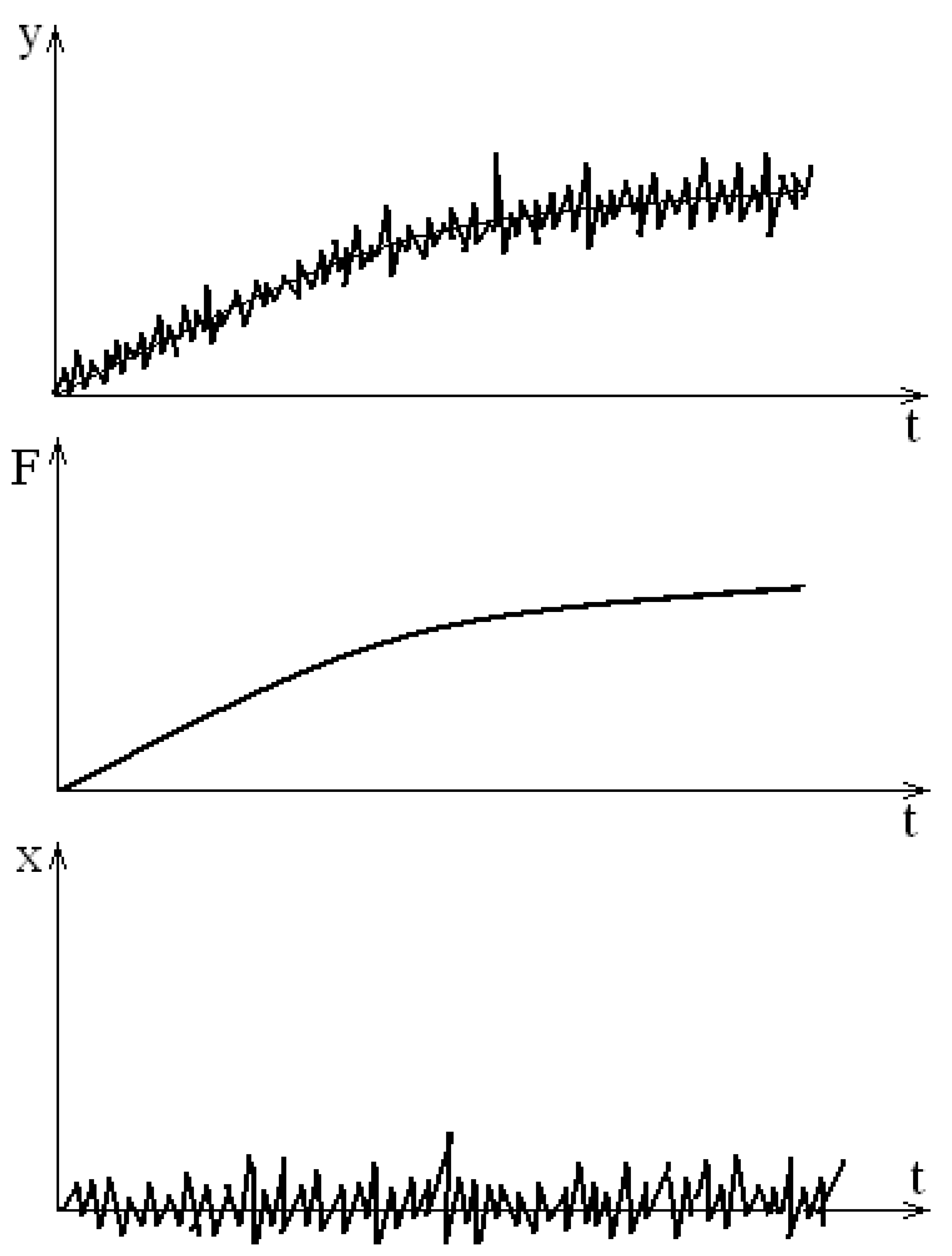
where F (t) is the non-stationary average of the measured random process, X (t) is the stationary random process (Figure 1).

To obtain an estimate of F (t), various methods of optimal filtering (for example, a Kalman-Bewsey filter) can be used. However, to build a filtering algorithm, a priori knowledge of the distribution function type and spectral density of the process is necessary. In addition, filtration methods do not allow obtaining estimates of other probabilistic characteristics of the stationary component. Such a setting of the task may be sufficient in cases where only information about the average value F (t) is needed, but for the purposes of complete processing, it is necessary to obtain information about the component of the process X (t).

In such cases, it is possible to construct algorithms for estimating the probabilistic characteristics of a non-stationary random process using non-parametric statistics.

It is known [8,9] that non-parametric statistics call some function of a random variable with an unknown probability distribution. This function itself has a known distribution, the properties of which in some way characterize the properties of an unknown distribution of the original random variable. Knowing the distribution of non-parametric statistics, you can use it to formulate and test different hypotheses about the properties of unknown distributions (for example, their symmetry, stationary, and so on).

2. Material and methods

Consider the most common non-parametric statistics.

Let Y = {y₁, y₂,…………y_n} - be a vector of sample values from the process y (t), obtained by sampling it in time in an interval of ∆t, with ∆t > τ_k, where τ_k is the correlation interval of the process. Let us determine the sign function of observations in the form

s i g n \begin{matrix}  \end{matrix} y = \frac{y}{| y |} = {\frac{1}{- 1} \begin{matrix} , \\ , \end{matrix} \begin{matrix}  \end{matrix} \begin{matrix} y \geq 0 \\ y < 0 \end{matrix}

(2)

Let's introduce a unit jump function or a positive sign vector

u (y) = {\begin{matrix} 1 \\ 0 \end{matrix} \begin{matrix} , \\ , \end{matrix} \begin{matrix}  \end{matrix} \begin{matrix} y \geq 0 \\ y < 0 \end{matrix}

(3)

related to the sign function by the relation

2u(y) = sign y + 1.

Functions (2) and (3) are called sign statistics or elementary inversions, and the vector

\bar{U} (y) = {u_{1} (y), u_{2} (y), \dots, u_{n} (y)},

composed of sign statistics called a sign vector.

The distribution of sign statistics is binomial with parameter

n

equal to the sample size:

P_{n} (u = i) = C_{i}^{n} p^{i} q^{n - i} .

(4)

The mean and variance of sign statistics are defined as

M_{u} = n p

D_{u} = n p q

, respectively. The parameter P of this distribution is the probability of sign statistics appearing in a single test.

If you rearrange the

\bar{Y}

sample items in ascending order

\bar{Y} = {y^{(1)}, y^{(2)}, \dots \dots y^{(n)}},

(5)

where y^(k) ≤ y^(j) for k < j, then we get a vector called the vector of ordinal statistics, and its elements y^(k) are ordinal statistics. When replacing the elements of the sample y^(k) with their ranks R_k, where R_k = К is the ordinal number of the element y^(k) in the ranked series, we obtain the vector

\bar{R} (\bar{y}) = {R_{1,} R_{2,} \dots, R_{n}}

, called the rank vector. If you need to have both information about the rank R of the sample value and its ordinal number

i

in the original sample, then you can enter the designation

R_{i}

, which means that R is the rank of the

i

-th observation in the sample. It is believed that

n

is known and fixed.

Let's consider the nature of specific problems solved using non-parametric methods. First of all, this task of estimating unknown distributions, which differs from the problem of approximating an unknown distribution by known functions, considered in ordinary statistics. In a non-parametric formulation, this problem can be formulated as an estimate of the difference between an unknown distribution and a given class of distributions. If it is necessary to specify these differences, the task of estimating the parameters of distributions is formulated. In this case, not the parameter itself is evaluated, but the parameter of difference between distributions within a given non-parametric class. Another category of non-parametric problems is testing non-parametric hypotheses. In any nonparametric hypothesis testing problem consisting of two competing hypotheses, the alternative is always nonparametric, and the null hypothesis can be either simple or nonparametric. The difference between hypotheses is not related to a specific type of distribution function, since one of the hypotheses has a class of unknown distributions. The essence of the procedure is that based on the original sample, it is necessary to attach an algorithm, the result of which will be a decision on the truth of one of the hypotheses.

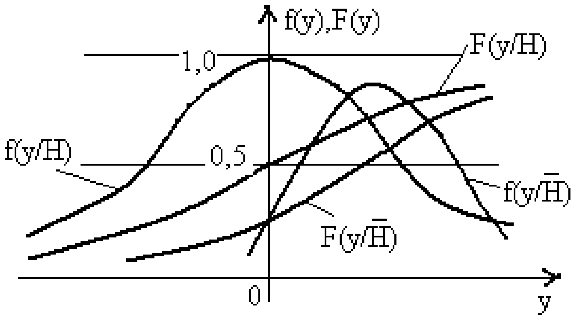
Consider, for example, the procedure for generating decision rules to test the symmetry hypothesis of the distribution of some random variable

y

(Figure 2), using sign statistics (3) for this.

Let's enter the character counter function into consideration

Z = \sum_{i = 1}^{n} u_{i} (y_{i}),

which has a binomial distribution according to formula (3).

As can be seen from Figure 1 for symmetrical distribution P = 0.5, and for asymmetrical distribution P ≠ 0.5.

Let's introduce the main hypothesis about the symmetry of the distribution

H: f(y) = f(-y), or P = 0.5

and an alternative hypothesis - about its asymmetry

\bar{H} f (y) \neq f (- y), or P \neq 0.5

Given that with sample volumes of

n

> 20, the binomial distribution is well approximated by the Gaussian distribution, the decisive rule on the Neumann-Pearson criterion can be written as follows: if Z > C₁ is true to the alternative hypothesis; if Z < C₁ is true to the basic hypothesis. At the same time,

C_{1}

is the threshold of the decisive rule:

C_{1} = \frac{Z_{α}}{2} \sqrt{n} + \frac{n}{2} - 1 .

(6)

The value of the threshold of the decisive rule is selected from the following condition, which can be found in [10,11]

α = 1 - F [\frac{C_{1} + 1 - \frac{n}{2}}{\frac{\sqrt{n}}{2}}] .

(7)

Here

α

is a Gaussian distribution parameter called the significance level (in literary sources this parameter is often called the probability of error of the first kind, or the "probability of false alarm"), and

n

- as already noted, is the sample size.

Such a decisive rule is unbiased only for a P > 0.5. At P < 0.5, the decisive rule Z < C2 turns out to be unbiased, where the threshold

C_{2} = \frac{Z_{1 - α}}{2} \sqrt{n} + \frac{n}{2} - 1 .

(8)

In this case, the probabilities of error of the second kind (signal skipping) is determined from the following relationships:

β_{1} = F [\frac{Z_{α / 2} - \sqrt{n} (p - 0.5)}{\sqrt{p q}}];

(9)

β_{2} = F [\frac{Z_{1 - α / 2} - \sqrt{n} (p - 0.5)}{\sqrt{p q}}],

(10)

which are described in [1,12].

With small volumes of observations (n < 20), the value of the

α

significance level can be determined according to the Bernoulli distribution

α = P (y > C_{1} | H) = \sum_{m = C_{1}}^{n} {C_{n}}^{m} {0.5}^{m} {0.5}^{n - m},

(11)

where the value of the С₁ threshold is determined. Error amount of the second kind in this case will be determined from the relation

β_{1} = P (y > C_{1} | \bar{H}) = \sum_{m = 0}^{m = C_{1}} {C_{n}}^{m} p^{m} {(1 - p)}^{n - m},

if the distribution parameter P > 0.5. In the same case, when P < 0.5, the amount of the error of the second kind should be defined as

β_{2} = P (y > C_{2} | \bar{H}) = \sum_{m = C_{2}}^{n} {C_{n}}^{m} p^{m} {(1 - p)}^{n - m} .

(13)

Percentage points as well as distributions of various modifications of variable (11) can be found in works [1,13].

3. Theory/Calculation

Let's consider the possibility of using non-parametric methods of decision theory to estimate the probabilistic characteristics of non-stationary random processes described by the model (1) (Figure 1). By probability characteristics we will mean the mean value, variance (standard deviation), distribution function and correlation function. Recall that a random process represented by a single implementation is considered in conditions of a priori uncertainty about the type of distribution function. To estimate the probabilistic characteristics of such a random process, it is advisable to first identify a non-stationary average F (t) (obtain an estimate of the average value), and then obtain estimates of other probabilistic characteristics of the component X (t).

To increase the accuracy of the separation of the non-stationary component of the random process, it is desirable to divide the entire observation interval into stationary intervals, the length and number of which are determined by the type of non-stationary component F (t) and the probabilistic characteristics of the stationary component X (t). To divide the observation interval into stationary intervals, we will use well-known in the literature Kendall's statistics [14]

T^{2} = \sum_{i = 1}^{n - 1} \sum_{k = i + 1}^{n} u (y_{i}, y_{k})

(14)

where:

u (y_{i}, y_{k}) = {\begin{matrix} 1 \\ 0 \end{matrix} \begin{matrix} , \\ , \end{matrix} \begin{matrix} y_{i} \geq y_{k} \\ y_{i} < y_{k} \end{matrix}

and are called sign statistics or elementary inversions. Here the

y_{i}

and

y_{k}

are values of the measured process obtained by sampling with a sampling interval of ∆t. The sampling interval in this case is selected based on the statistical independence of the two adjacent sample values

y_{i}

and

y_{i + 1}

that is, the

∆ t \geq τ_{k}

where

τ_{k}

- the random process correlation interval. The selection of the sampling interval is a separate task that needs to be solved.

Using Kendall statistics makes it quite easy to divide the time series of observations

y (t)

by the finite number of stationary intervals with a given probability

P = 1 - α

by parameters such as the average value

m [y (t)]

and variance

D [y (t)]

. Here α is the probability that the interval is not stationary. In Russian-language literary sources, α is commonly referred to as "the probability of a false alarm" or "the level of significance." The division procedure consists in calculating the current values

T^{2}

and the permissible limits

T_{m i n}^{2} [i; 1 - α / 2]

and

T_{m a x}^{2} [i; α / 2]

and in checking the stationarity condition by the Neumann-Pearson criterion [15,16,17]:

T_{m i n}^{2} < T_{i}^{2} \leq T_{m a x}^{2} .

(15)

The distribution of the Kendall variable for sample sizes

n > 10

differs little from the Gaussian distribution [14].

The values of the permissible limits of the decision rule thresholds can be determined from the relations

T_{m i n}^{2} = M [T^{2}] - x_{α / 2} \sqrt{D [T^{2}],}

(16)

T_{m a x}^{2} = M [T^{2}] + x_{α / 2} \sqrt{D [T^{2}],}

(17)

where

x_{α / 2}

is the percentage point of the Gaussian distribution.

Kendall's statistics are symmetrical about his mathematical expectation, since it is indifferent how elementary inversions are obtained: by fulfilling the inequality

y_{i} < y_{j}

y_{j} < y_{i}

with

j = i + 1, i + 2, i + 3 \dots .

This fact means that in many practical applications, a reverse procedure can be used, which gives tangible advantages in efficiency and other indicators.

The reversibility of the procedure can be used to divide time series into stationary intervals, at which the line of current values of

T^{2}

is sequentially reflected from permissible boundaries. In this case, it is necessary to constantly take into account the moments of transition of the sign function

u (y)

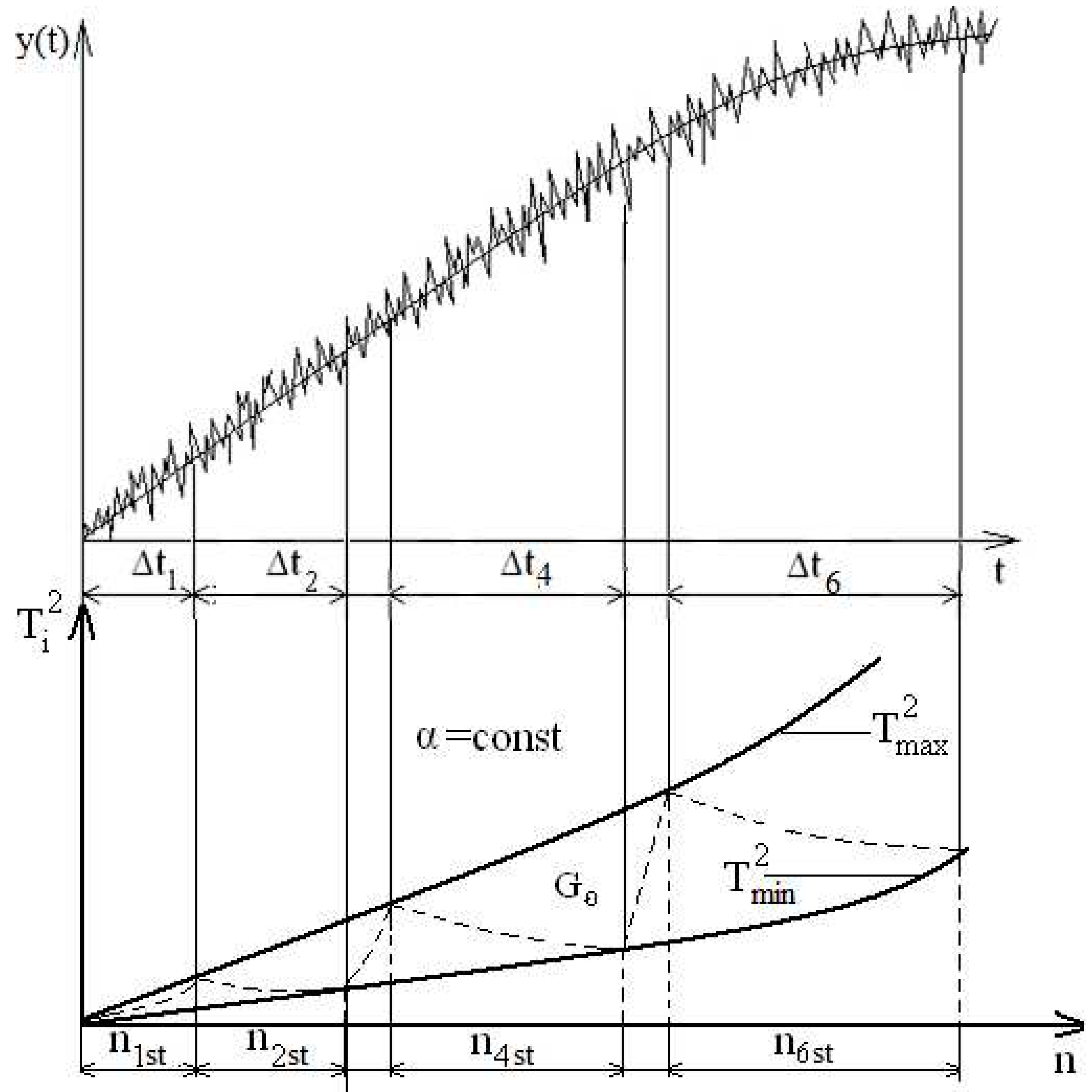
to the opposite value, that is, to fix the reflection points of total inversions from permissible boundaries. As in previous cases, non-stationary measurement data are divided into stationary at some intervals, the statistical characteristics of which are constant but not equal to each other. Consider the method of reflected inversions in more detail (Figure 3).

According to incoming samples

y_{1}, y_{2}, \dots y_{n}

of the measured series y (t) calculates the function

u (y_{i}, y_{j})

from which Kendall statistics are determined. Valid bounds

T_{m a x}^{2}

and

T_{m i n}^{2}

are defined for a given significance level

α

. As well as in above the described methods, comparison of

T_{i}^{2}

with

T_{m a x}^{2}

and

T_{m i n}^{2}

as a result of which there can be two outcomes is made:

1. Inequality (15) is performed and the process does not leave the field of stationary;

2. Inequality (15) is broken and the process leaves the field of stationary.

The point corresponding to the moment of crossing the line

T_{i}^{2}

from one of the permissible boundaries is fixed, and the sign function

u (y_{i}, y_{j})

is "flipped" to the opposite value, as a result of which an fracture point is formed on the line

T_{i}^{2}

and the calculation process is repeated. When the second of the permissible boundaries is reached, the function

u (y_{i}, y_{j})

is again flipped while fixing the fracture point on the line

T_{i}^{2}

. Thus, the line

T_{i}^{2}

is all the time inside the stationary area and consistently reflected from the permissible boundary lines.

After determination of stationary sections probabilistic characteristics of measured non-stationary random process are evaluated. Evaluation is carried out on each stationary site separately.

Simplification of estimates of probabilistic characteristics is possible when using ordinal statistics (OS) of a ranked series when ranking the data obtained on the stationarity interval, in decreasing or increasing order:

x_{(1)} \leq x_{(2)} \leq \dots \leq x_{(R)} \leq \dots \leq x_{(N)}

(18)

In a number of works [18,19], studies of errors in estimating probabilistic characteristics by ordinal statistics were carried out. However, these works were limited to the study of a stationary stochastic process, while obtaining estimates of probabilistic characteristics from samples of a non-stationary stochastic process is of particular interest.

Application of ordinal statisticians allows to use simple enough procedures for the average estimation, based on central ordinal statistics (COS) ranked beside [20,21].

{\tilde{m}}_{11} = x_{(c)}; {\tilde{m}}_{12} = x_{(c + 1)}; {\tilde{m}}_{21} = \frac{1}{2} (x_{(c - 1)} + x_{(c)});

{\tilde{m}}_{22} = \frac{1}{2} (x_{(c)} + x_{(c + 1)}); {\tilde{m}}_{2 j} = \frac{1}{2} (x_{(c)} + x_{(c + j)});

{\tilde{m}}_{31} = \frac{1}{3} (x_{(c - 1)} + x_{(c)} + x_{(c + 1)}) .

There are estimates based on the truncation ranked series

{\tilde{m}}_{41} = \frac{1}{N - 2} \sum_{i = 2}^{N - 2} x_{(i)}; {\tilde{m}}_{4 j} = \frac{1}{N - j} \sum_{i = j}^{N - j} x_{(i)};

And also using extreme ordinal statistics

{\tilde{m}}_{51} = \frac{1}{2} (x_{(N)} + x_{(1)}); {\tilde{m}}_{52} = \frac{1}{2} (x_{(N - 1)} + x_{(2)});

{\tilde{m}}_{j} = \frac{1}{2} (x_{(N - j + 1)} + x_{(j)}) .

The estimations using various combinations of enumerated estimations can be synthesised:

{\tilde{m}}_{61} = \frac{1}{2} (x_{(K 1)} + x_{(K 2)}),

where

K 1 = E [0.73 N]

K 2 = E [0.23 N]

;

{\tilde{m}}_{62} = \frac{1}{2} (x_{(K 1)} + x_{(K 2)}),

where

K 1 = E [0.75 N]

K 2 = E [0.25 N]

;

{\tilde{m}}_{71} = v_{1} \cdot x_{(K 1)}; {\tilde{m}}_{72} = v_{1} \cdot x_{(K 1)} + v_{2} \cdot x_{(K 2)};

{\tilde{m}}_{7 j} = v_{1} \cdot x_{(K 1)} + v_{2} \cdot x_{(K 2)} + … v_{j} \cdot x_{(K j)}, j < < N;

{\tilde{m}}_{81} = v_{12} \cdot x_{(K 1)} + v_{2} \cdot x_{(K 2)}

{\tilde{m}}_{82} = v_{12} \cdot (x_{(K 1)} + x_{(K 2)}) + v_{34} \cdot (x_{(K 3)} + x_{(K 4)});

{\tilde{m}}_{8 j} = v_{12} \cdot (x_{(K 1)} + x_{(K 2)}) + … v_{i j} \cdot (x_{(K i)} + x_{(K j)});

The most optimal procedure for estimating the mean is an estimate based on the central ordinal statistics (COS) of the ranked series [22,23,24]:

{\tilde{m}}_{11} = x_{(c)};

(19)

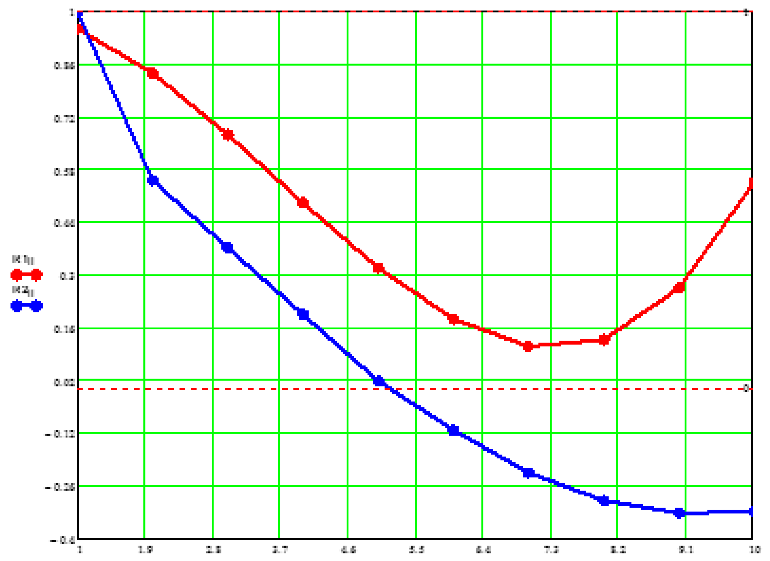
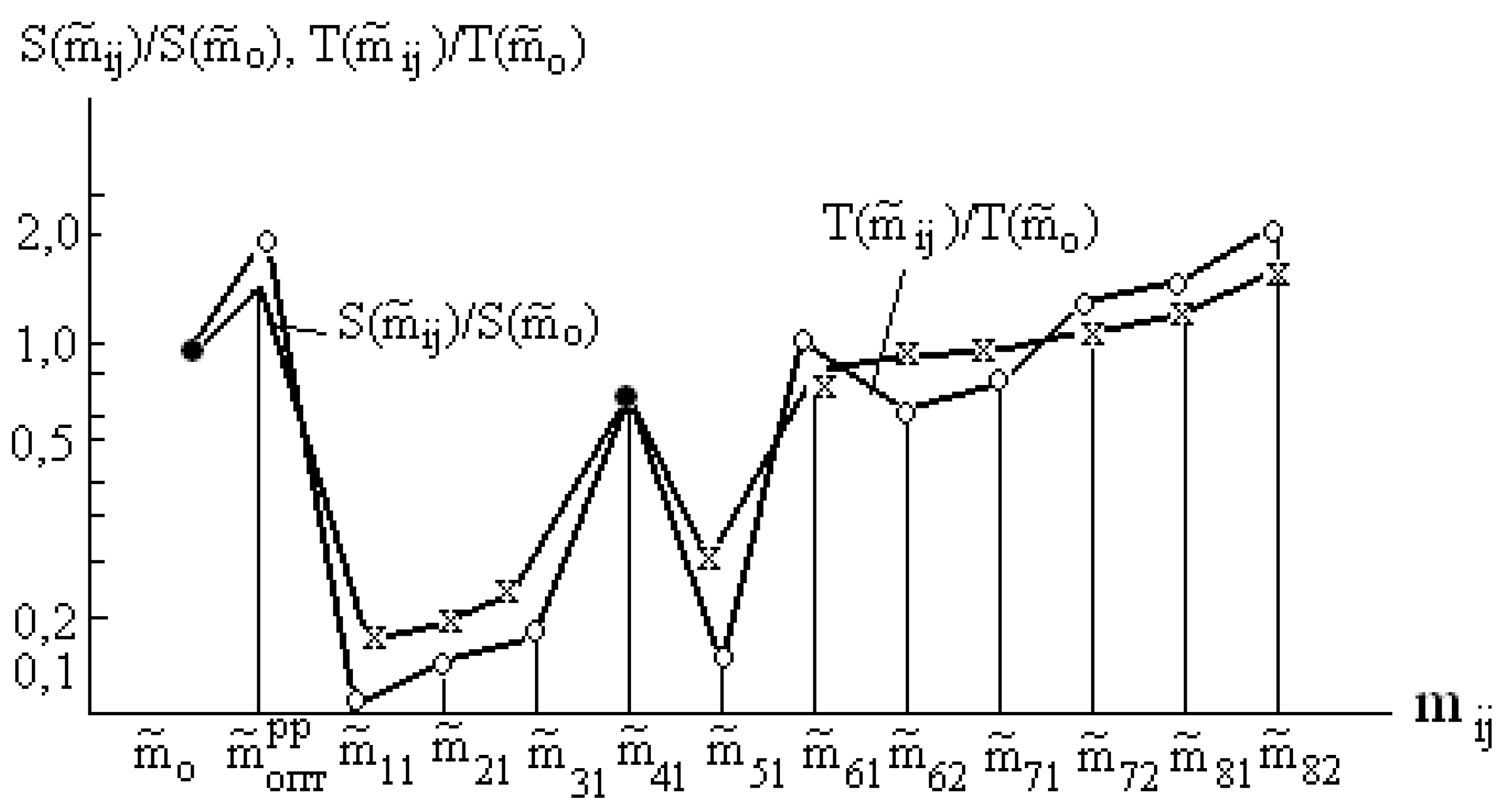
Obviously, that central ordinal statistics are most simple in implementation. On Figure 4 the comparative analysis of computing costs (memory size

S

and average calculation time

T

) of various modes of an estimation of the mean is shown (

S ({\tilde{m}}_{0})

and

T ({\tilde{m}}_{0})

- the memory size and the average calculation time when using the maximum likelihood estimate). The minimum costs, apparently, have estimations of an aspect

{\tilde{m}}_{11}

When measuring variance, it is advisable to use the same ranked series of ordinal statistics as when estimating the mean. At the same time, it is best to estimate not the variance of the process itself, but the standard deviation. To estimate the standard deviation in nonparametric statistics, there are used the simplest range functions span

W_{1} = x_{(N)} - x_{(1)}

and under the scope

W_{j} = x_{(n - j + 1)} - x_{(j)}

, using extreme order statistics ranked series:

\begin{array}{l} {\tilde{σ}}_{11} = ν (x_{(N)} - x_{(1)}), \\ {\tilde{σ}}_{12} = ν (x_{(N - 1)} - x_{(2)}) \end{array}

It is possible to use estimations also:

σ_{3 j} = ν (x_{(K 1)} - x_{(K 2)})

where for

σ_{31}

K 1 = E [0.75 N]

K 2 = E [0.25 N]

;

and for

σ_{32}

K 1 = E [0.73 N]

K 2 = E [0.25 N]

;

σ_{5} = ν (x_{(K 1)});

σ_{52} = v_{12} (x_{(K 1)} + x_{(K 2)}) + v_{34} (x_{(K 3)} + x_{(K 4)});

σ_{5 j} = v_{1} x_{(K 1)} + v_{2} x_{(K 2)} + … + v_{j} x_{(K j)} + …

As in the case of estimating the mean, the different combinations of central order statistics and extreme order statistics (EOS) are possible:

σ_{4 j} = ν (x_{(c + j)} - x_{(c - j)})

σ_{2 j} = ν (x_{(N - j + 1)} - x_{(c - j + 1)})

The coefficient

ν

can be assigned from a wide range, however, the most effective factor values are as follows:

ν = 1; ...1 / 2; ...1 / 3; ...1 / 4;

The optimal estimate of the variance is an estimate of the type

{\tilde{σ}}_{11} = ν (X_{(N)} - X_{(1)}) .

(20)

The optimal estimation conditions can be written in the following form [22,23,24]

{\tilde{σ}}_{o p t} = {\tilde{σ}}_{11} = ν (X_{(N)} - X_{(1)}), \{\begin{matrix} ν = \frac{1}{3}, N < 15 \\ ν = \frac{1}{4}, N \geq 15 \end{matrix}

(21)

The ranked series of ordinal statistics can be used to estimate the distribution function

F (x)

and the probability density function

f (x) .

In this case, it is enough to estimate one of them and indirectly obtain an estimate of the other, respectively by differentiating

F (x)

or integrating

f (x) .

With regard to the technique of transmission of telemetry data it is better assess the distribution function F(x) because of the greater complexity in the implementation of methods for estimating f(x) and better noise immunity transfer F(x) compared to f(x) because of the continuous increase in the ordinate F(x). Therefore, consideration of methods of estimating the distribution function be paid more attention.

The classic definition of the distribution function, as the probability of the event (x(t) < x) allows us to write the following relation

{\tilde{F}}_{0} (x) = Prob (x (t) < x) = \frac{N_{x}}{N} = \frac{1}{N} \sum c (x - x_{i}),

where - Prob(…) means probability, N - sample size,

N_{x}

- number of samples of the process x(t), not exceeding the value of x,

c (x - x_{i})

- the comparison function.

c (x - x_{i}) = {\begin{matrix} 1, \\ 0, \end{matrix} \begin{matrix} x \geq x_{i} \\ x < x_{i} \end{matrix}

Statistical relationship between the sample value and its rank allows us to write the following approximate value:

{\tilde{F}}_{1} (x) = {\tilde{F}}_{1} (x_{(R)}) = \frac{R}{N + 1} .

Modification of this method, based on fixation as quantile not order statistic x(R) of rank R, while a linear combination of Q of order statistics x(R) of rank R, while a linear combination of Q of order statistics

x_{(R)}^{Q} = \sum_{q = 1}^{Q} A_{q} x_{(q)}

allow to generate the following estimates

\begin{array}{l} {\tilde{F}}_{2} (\frac{1}{2} (x_{(R - 1)} + x_{(R)})) = \frac{R}{N + 1}; \\ {\tilde{F}}_{3} (\frac{1}{2} (x_{(R)} + x_{(R + 1)})) = \frac{R}{N + 1}; \\ {\tilde{F}}_{4} (\frac{1}{3} (x_{(R - 1)} + x_{(R)} + x_{(R + 1)})) = \frac{R}{N + 1} . \end{array}

At these estimations in the capacity of a quantile magnitude, average of two or three ordinal statisticians is fixed.

Other mode of the estimation of a cumulative distribution function is based on the evaluation of a nonparametric tolerant interval (L2 − L1) where L1 and L2 name 100

β

-percent independent of distribution F(x) tolerance limits at level

γ

and

Prob [(F_{(L 2)} - F_{(L 1)}) \geq β] = γ

If to suppose L1 = x (R), and L2 = x (S), where R < S the tolerant interval [x(R), x(S)] is equal to the sum of elementary shares from R-th to S-th, i.e.

\begin{array}{l} Prob [(F_{(x_{(R)} - x_{(S)})} \geq β] = γ = \frac{N!}{(S - R - 1)! (N - S + R)!} \times \int_{β}^{1} Z^{S - R - 1} {(1 - Z)}^{n - S - R} d z = \\ = 1 - I_{β} (S - R, N - S + R + 1) = \sum_{i = 1}^{S - R - 1} (\begin{matrix} N \\ i \end{matrix}) β^{i} {(1 - β)}^{N - i} . \end{array}

Thus

γ

is a function of arguments N, S-R and

β

. There is some minimum value Nmin to which in each specific case there matches quite certain combination R and S. It is possible to determine

\frac{1}{2} N (N - 1)

tolerant intervals with various level

γ

among which N/2 and N (N−1)/2 (depending on that even or odd N) will be symmetric. For security of symmetry of a rank should be connected a condition:

S = N - R + 1 .

Then for an estimation of cumulative distribution function F₅(x) in points x(R) and x(S) with a confidence coefficient

γ

is possible to accept the following magnitudes:

\begin{array}{l} F_{5} (x_{(R)}) = \frac{1 - β (R, S)}{2}, \\ F_{5} (x_{(S)}) = \frac{1 + β (R, S)}{2} . \end{array}

Thus, changing value R from 1 to N/2 and computing matching values S, it is possible to gain estimation F₅(x) in N points.

One more mode of nonparametric estimation F₆(x) can be generated from definition of a nonparametric confidence interval [

x_{(R)}

x_{(R + K)}

] for a quantile x_p level p. The Confidence level

γ

is determined from a relation:

γ = Prob ({\tilde{F}}_{6} (x_{(R)})) \leq p \leq F_{6} (x_{(R + K)}) = I_{p} (R, N - K + 1) - I_{p} (R + K, N - R - K + 1),

where

I_{p} (n, m)

– Prison’s incomplete Beta -function

I_{p} (n, m) = \frac{Г (n + m)}{Г (n) \cdot Г (m)} \int_{O}^{P} x^{n - 1} {(1 - x)}^{m - 1} d x .

And the probability [gamma] that the quantile х_р will appear between ordinal statistics

x_{(R)}

and

x_{(R + K)}

does not depend on an aspect of initial distribution F(x).

The statistical relationship between the sampled value and its rank allows to write the following approximate value [22,23]:

{\tilde{F}}_{1} = {\tilde{F}}_{1} (x_{(R)} = \frac{R}{N + 1},

(22)

where

R

is the rank or rank statistics (number in the ranked row) of the element

x_{(R)} .

A ranked series of ordinal statics can also be used to estimate the correlation function of a random process.

To evaluate the correlation function in real time, the most interesting are fairly simple rank and sign non-parametric methods of estimation [20], in particular, the methods of Spearman

ρ_{s p}

and Kendall

ρ_{k}

ρ_{s p} (j) = 1 - K_{s p} (N) \sum_{i = 1}^{N} P_{R}^{2} j);

(23)

ρ_{k} (j) = K_{k} (N) \sum_{i = 1}^{N - 1} R_{i} - 1 .

Here

P_{R}

is the difference between the elements

x_{i}

and

x_{(i + j)}

;

K_{s p} (N)

- Spearman constant (at

N = c o n s t

K_{s p} = 6 / (N^{3} - N)

);

R_{i}

- rank of the

i

-th element

x_{i}

;

K_{k}

(N)

- Kendall constant (at N = const,

K_{k}

4 / (N^{2} - N)

). The procedures for estimating the correlation function according to the above formulas allow a significant simplification due to the table setting of coefficients

K_{s p} (N)

and

K_{k}

(N)

and the value

P_{R}^{2} (j)

in the microcomputer ROM (at a fixed interval of local stationary).

4. Discussion and results

Analysis of errors in estimates of probability characteristics of a random process using the method of reflected inversions was carried out using the method of statistical modeling on PC using Mathcad.

Consider a random function with a Gaussian distribution.

A random process, white noise

x_{t}

is generated (a vector of N random numbers having a Gaussian distribution):

x_{t} = r n o r m (N, μ, σ) .

A signal (trend) of the form

F_{t} = 5 (1 - e^{(- 0.01 t)})

was superimposed on a random function.

As a result, a non-stationary random process of the form

y_{t} = x_{t} + F_{t}

was generated.

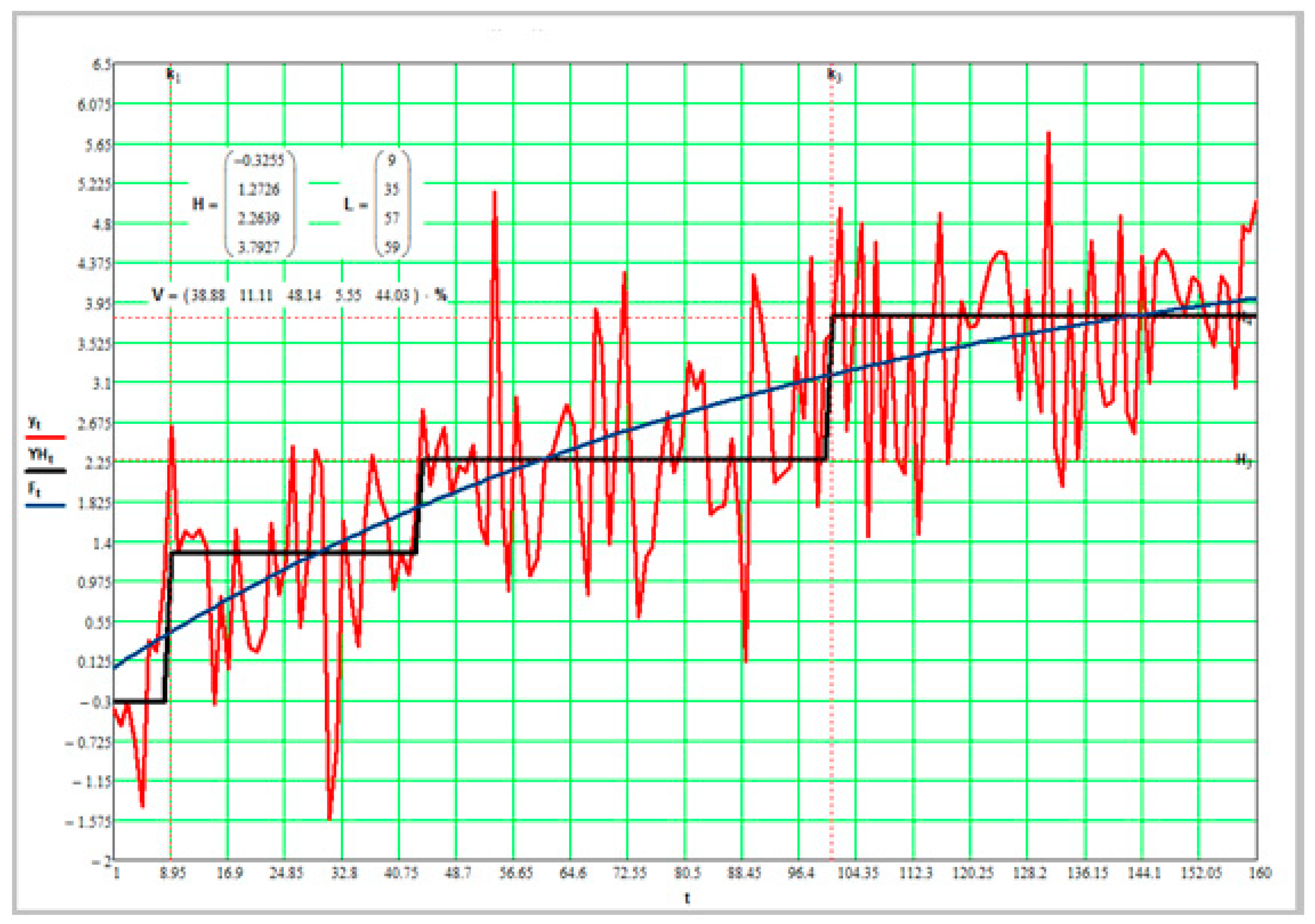
Figure 5 shows an example of a simulation.

In the figure, the simulated random process

y_{t}

is shown in red, the trend

F_{t}

- in blue, the average estimate calculated by the formula (19) - in black.

In the figure, we have four stationary sections with a length of 9 samples, 35 samples, 57 and 59 reports, respectively.

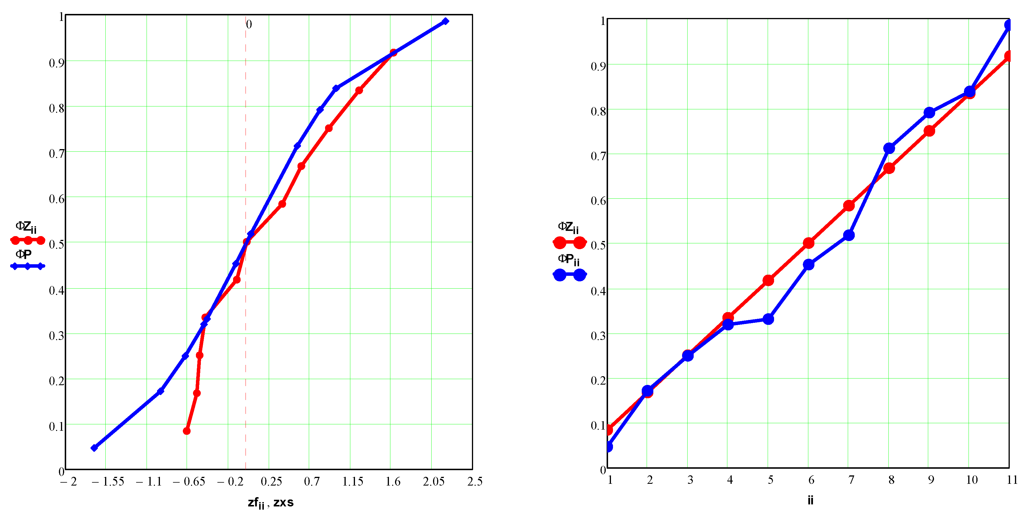
The estimation of the distribution function (red) and its comparison with the given one (blue) are shown in Figure 6.

Unfortunately, with this approach, it is not possible to obtain estimates of the correlation function, since obtaining the above estimates is associated with the requirement of statistical independence between the counts. Thus, an estimate of the correlation function must be obtained separately from estimates of other probabilistic characteristics of the random process.

To evaluate the correlation function, a random process with a correlation function of the following form was modeled:

R_{x} = σ^{2} \cdot e x p (- α |τ|) .

Figure 7 shows the estimate of the correlation function (red) compared to the given (blue). Correlation function was evaluated using formula (24).

Random functions with the following distribution function were also used for modeling:

rexp (N, r) - generates the vector N of random numbers that have an exponential distribution. r > 0 - distribution parameter (e.g. r = 0.9);

runif (N, a, b) - generates the vector N of random numbers having a uniform distribution in which b and a are boundary points of the interval. a < b. (e.g. a = -1, b = 1);

rt (N, d) - Student distribution, where N is the number of random numbers, d is the distribution parameter, d > 0.

The results of statistical modeling showed that the method is quite effective. Modeling was carried out for various types of trends: exponential, oscillatory, linear. Also, the parameters of the algorithms varied, such as the signal-to-noise ratio (the ratio of the trend amplitude to the dispersion of the random component), the sampling interval, the value of the α significance level. The error in the estimate of the average value, as a rule, does not exceed 7%, and the variance and distribution function - 10%. Errors in correlation function estimates do not exceed 18%, which is an acceptable result for data processing purposes, for example, in radio-telemetry systems of spacecraft [24,25,26].

Figure 7. Estimation of correlation function.

Thus, applying the best estimates of the form (19), (20), (22-24) allows the same ranked series of ordinal statistics to be used to estimate such different probabilistic characteristics of the random process as the mean, variance, distribution function and correlation function. This fact is very important, since it allows, firstly, to significantly reduce the computational cost of obtaining these estimates, and secondly, it allows you to obtain almost complete information about the measured process in one dimension.

Of particular interest is the formation of output streams of compressed data obtained in accordance with expression (19) and their connection to the communication channel. Some aspects of this problem are covered, for example, in [27].

5. Conclusions

This article discusses how to evaluate the probabilistic characteristics of transient broadband random processes. Very often, a feature of random processes is that they are represented by a single implementation under conditions of a priori uncertainty about the type of distribution function. Since the use of traditional methods of mathematical statistics to calculate the probabilistic characteristics of such random processes is not possible, the use of non-parametric methods of decision theory has been proposed. The essence of the proposed methods consists in using Kendall's nonparametric statistics to divide the entire measurement interval into stationary intervals, followed by calculating probability characteristics at each stationary interval. By probability characteristics we will mean the mean value, variance (standard deviation), distribution function and correlation function. To calculate probability characteristics, ordinal and rank statistics (19) - (24) of the ranked series are used, which are very easy to calculate. It is important to keep in mind that the same ranked series is used to calculate all probability characteristics (except the correlation function). This leads to a significant reduction in computational costs, since the ranking procedure is applied only once, and the entire set of necessary probabilistic characteristics is calculated.

The article presents the results of computer modeling. Analysis of errors in estimates of probability characteristics of a random process using the method of reflected inversions was carried out using the method of statistical modeling on PC using Mathcad. Random processes with various distribution functions, such as Gaussian distribution, exponential distribution, Student distribution, uniform distribution, were studied in the simulation. The function

F_{t} = 5 (1 - e^{(- 0.01 t)}

) was investigated as a trend. To evaluate the correlation function, a random process with a correlation function of the form

R_{x} = σ^{2} \cdot e x p (- α |τ|)

was modeled.

Funding

This research received no external funding.

Institutional Review Board Statement

Not applicable.

Informed Consent Statement

Not applicable.

Data Availability Statement

Not applicable.

Acknowledgments

The author of the article expresses sincere gratitude to the scientists and specialists of the departments “Radio-electronic systems and devices”, “Information systems and telecommunications” of N. Bauman Moscow State Technical University, whose consultations and advices were taken into account when performing scientific research, the results of which are presented in this article.

Abbreviations

The following abbreviations are used in this manuscript:

COS	central ordinal statistics
EOS	extreme order statistics

References

Francisco Colodro, Juana María Martínez-Heredia, José Luis Mora, Antonio Torralba. Correction of errors and harmonic distortion in pulse-width modulation of digital signals. International Journal of Electronics and Communications. Volume, 142, December 2021, 153991. [CrossRef]
Younes Naderi-Gavareshki, Hassan Khani, Ehsan Rahiminejad. Improved coded/uncoded monobit receiver for transmit-reference UWB communication systems: Performance evaluation and digital circuit design. International Journal of Electronics and Communications. Volume 127, December 2020, 153460. [CrossRef]
Salamon D. Compression of data, images and a sound. Moscow: Technosphere; 2004, 368p.
Ivanov V.G., Lomonosov U.B., Lyubarsky M.G. Analysis and classification of methods of compression of the information. Bulletin NTU KhPI. Thematic issue: Information science and modelling. No. 49. Kharkov; 2008, P. 78-86.
Luis Alberto Vasquez-Toledo, Berenice Borja-Benítez, Ricardo Marcelin-Jiménez, Enrique Rodríguez-Colina, José Alfredo Tirado-Mendez. Mathematical analysis of highly scalable cognitive radio systems using hybrid game and queuing theory. International Journal of Electronics and Communications. Volume 127, 2020; 153406. [CrossRef]
Ringo J. Mixed-Signal Electronics Technology for Space (MSETS). Defense Technical Information Center; 2006, Feb 16. [CrossRef]
Horan S. Compression of Telemetry. Lossless Compression Handbook. Communications, Networking and Multimedia. 2003, P.247–253. [CrossRef]
F.P. Tarasenko. Nonparametric statistics. Tomsk: Tomsk University Publishing House. 1976, 294 p.
Efromovich S. On shrinking minimax convergence in nonparametric statistics. Journal of Nonparametric Statistics. Informa UK Limited; 2014 Jul 3; Volume 26(3), P. 555–573. [CrossRef]
Belous A.I., Solodukha V.A., Shvedov S.V. Space electronics. Moscow: Technosphere. 2015, 488 p.
Means of collecting information. Collecting Information SS. Routledge; 2007, Jun 1; P.51–55. [CrossRef]
Functions of random variables. Probability Theory and Statistical Applications. De Gruyter; 2016 Jul 11; P. 73–82. [CrossRef]
B.R. Levin. Theoretical foundations of statistical radio engineering. Moscow: Soviet radio. 1968, 512 p.
Functions of random variables. Probability Theory and Statistical Applications. De Gruyter; 2016 Jul 11; P. 73–82. [CrossRef]
Borodin A.N. Random processes. Textbook. St. Petersburg: Lan. 2013, 640 p.
Hsiao C, Zhou Q. Incidental Parameters, Initial Conditions and Sample Size in Statistical Inference for Dynamic Panel Data Models. SSRN Electronic Journal. Elsevier BV; 2018, P. 53. [CrossRef]
Hajek J, Sidak Z, Sen P. Elementary theory of rank tests. Theory of Rank Tests. Elsevier. 1999, P. 35–93. [CrossRef]
Spagnolini U. Random Processes and Linear Systems. Statistical Signal Processing in Engineering. John Wiley & Sons, Ltd. 2017, Dec 15; P. 63–82. [CrossRef]
Ivanov VG, Lyubarskiy MG, Lomonosov JV. Compression of Text Image Based on Selection of Characters and Their Classification. Journal of Automation and Information Sciences [Internet]. Begell House, Volume 42(11). 2010, P. 46–57. [CrossRef]
G. David. Ordinal statistics. Moscow: Science. 1979, 336 p.
Manfred Stommel, Katherine J. Dontje. Nonparametric/Ordinal Statistics. Statistics for Advanced Practice Nurses and Health Professionals. Springer Publishing Company. 2014, 352 p. [CrossRef]
Yesmagambetov B.-B.S., Inkov A.M. Fast changing processes in radiotelemetry systems of space vehicles. Journal of Systems Engineering and Electronics. Vol. 26, No. 5. Beijing. 2015, p.941-945. [CrossRef]
Yesmagambetov B.-B.S. Statistical data processing in radio telemetry systems. Bulletin of N. Bauman Moscow State Technical University. Series of instrumentation. No. 1. Moscow. 2015, p. 13-21.
Nazarov A.V., Kozyrev G.I., Shitov I.B., et al. Modern telemetry in theory and practice. Training course. St. Petersburg: Science and technology. 2007, 679 p.
Krejcar O. Modern Telemetry. InTech. 2011 Oct 5; 600 p. [CrossRef]
Stacey D. Aeronautical Radio Communication Systems and Networks. John Wiley & Sons, Ltd. 2008 Feb 22, 350 p. [CrossRef]
B. Yesmagambetov, A. Mussabekov, N.Alymov, A.Apsemetov, M. Balabekova, K. Kayumov, K. Arystanbayev, A. Imanbayeva. Determination of Characteristics of Associative Storage Devices in Radio Telemetry Systems with Data Compression. Computation 2023, Volume 11, Issue 6, 111. Basel, June. [CrossRef]

Figure 1. Non-stationary random process model.

Figure 2. Testing the distribution symmetry hypothesis.

Figure 3. Division of observation interval into stationary intervals.

Figure 4. The comparative analysis of computing costs of an estimation.

Figure 5. Modeling a random process with a Gaussian distribution.

Figure 6. Estimation of distribution function.

Disclaimer/Publisher’s Note: The statements, opinions and data contained in all publications are solely those of the individual author(s) and contributor(s) and not of MDPI and/or the editor(s). MDPI and/or the editor(s) disclaim responsibility for any injury to people or property resulting from any ideas, methods, instructions or products referred to in the content.

© 2023 by the authors. Licensee MDPI, Basel, Switzerland. This article is an open access article distributed under the terms and conditions of the Creative Commons Attribution (CC BY) license (http://creativecommons.org/licenses/by/4.0/).

Copyright: This open access article is published under a Creative Commons CC BY 4.0 license, which permit the free download, distribution, and reuse, provided that the author and preprint are cited in any reuse.

MDPI Initiatives

Important Links

Choose an area of interest and we will send you notifications of new preprints at your preferred frequency.

Disclaimer

Determination of the Characteristics of Non-stationary Random Processes by Non-parametric Methods of Solution Theory

Abstract

1. Introduction

2. Material and methods

3. Theory/Calculation

4. Discussion and results

5. Conclusions

Funding

Institutional Review Board Statement

Informed Consent Statement

Data Availability Statement

Acknowledgments

Abbreviations

References

MDPI Initiatives

Important Links

Subscribe