CFD Analysis of Heat Transfer Enhancement for Twisted Tape Inserted in spirally Corrugated Tubes

Preprint

Article

CFD Analysis of Heat Transfer Enhancement for Twisted Tape Inserted in spirally Corrugated Tubes

Altmetrics

Downloads

101

Views

Comments

Mouhsine Benmbarek,

Samir Farid Moujaes^*

Mouhsine Benmbarek,

Samir Farid Moujaes^*

This version is not peer-reviewed

Submitted:

31 August 2023

Posted:

05 September 2023

You are already at the latest version

Alerts

Abstract

Abstract: In this study, a computational fluid dynamics (CFD) simulation was conducted to validate the CFD model with experimental data from Zimparov et.al (2012), which investigates the heat transfer performance in a spirally corrugated tube that has a twisted tape inserted. The heat transfer was then compared to a simple corrugated tube without the twisted tape and to a smooth tube with no corrugations and no twisted tape. This simulation is compared with a previous experimental study conducted by (Zimparov et al. 2012), which focuses on tubes with a height-to-diameter ratio e/Di > 0.04 and small relative pitches of the twisted tape, H/Di. The largest improvement was noticed in the tube with e/Di= 0.057 and ridge pitch-to-height ratio p/e=6.77 with a twisted tape of H/Di= 4.7. This tube is labeled 5035. Tube 5035 was found to have the most significant enhancement, hence the focus of the CFD simulation will be on this tube, and the simulation will range for Reynolds numbers, 3.5 x 103 < Re < 5.0 x 104. The focus of this simulation is the evaluation of heat transfer and friction factors; a metric was used to obtain an empirical representation of the tube’s performance. Keywords: Spirally corrugated tube; Twisted tape; Heat transfer enhancement; Friction factor; Nusselt number; Computational fluid dynamics (CFD); Star CCM+

Keywords:

Subject: Engineering - Mechanical Engineering

1. Introduction

The use and transfer of energy is necessary in our society today, but that does not come without drawbacks on our planet’s environment and our economy. Natural resources are decreasing, as is their cost to produce and transfer. Creating ways to maximize the energy transfer process is extremely valuable and one way to do so is to increase the performance of heat exchangers to reduce energy loss, costs, and materials [1]. One of the best methods to enhance heat transfer in heat exchangers is compound enhancement, which is when different enhancement techniques are used simultaneously. This particular field is promising for future development [2]. The heat transfer coefficient can be increased significantly using compound enhancement by inserting different devices into a modified tube [2]. The aim of this study is to create a CFD model that is reliable for future attempts at different geometries. Many researchers relied on experiments to develop these enhancements. Heat transfer is increased by corrugation in turbulent flow b increasing the turbulence level and breaking the boundary layer of the flow [3]. Many researchers started using computational methods since these have been developed over recent decades and different computational calculation methods were created. These new methods allow researchers in saving to save time and effort, as well as funds that would otherwise be needed to create experimental setups and structures [5]. Sparrow et al.(1983). [4] adopted a numerical simulation as early as the 1980s to simulate laminar flow in triangular corrugated tubes and study its heat transfer performance [5]. Rahman et.al (2013) used FLUENT to investigate the effect of a multi-start inner grooved tube on the flow of refrigerant R22. They found that the enhanced tube provided a higher heat transfer coefficient than smooth tubes. Rahimi et al. (2009) discusses an experimental and computational fluid dynamics (CFD) investigation on the heat transfer and friction factor characteristics of a tube with modified twisted tape inserts. The study aimed to investigate the effect of different modified twisted tape inserts on heat transfer enhancement and friction factor characteristics. The experimental setup involved a horizontal test section with a heated tube and a modified twisted tape insert. The modified twisted tapes were made of aluminum and had various modifications to the geometrical parameters, such as tape width, twist ratio, and cut angles. The heat transfer coefficient and friction factor were measured experimentally, and CFD simulations were also carried out to validate the experimental results, which showed that the modified twisted tape inserts significantly enhanced the heat transfer coefficient and friction factor compared to the plain tube. Furthermore, the CFD simulations agreed well with the experimental data. The study also investigated the effect of different flow rates on the heat transfer and friction factor characteristics. It was found that increasing the flow rate increased the heat transfer coefficient and friction factor for all the modified twisted tape inserts. In conclusion, the study showed that the modified twisted tape inserts can significantly enhance the heat transfer coefficient and friction factor of a tube. The results can be useful for the design of heat exchangers and other thermal systems where heat transfer enhancement is important [11].

Lou et al. (2011) conducted a simulation study of heat transfer tubes equipped with twisted-tape inserts, which are commonly used in heat exchangers to enhance heat transfer. The simulations were conducted using computational fluid dynamics (CFD) techniques to investigate the effects of different twisted-tape geometries on heat transfer and fluid flow characteristics. The study found that the twisted-tape inserts significantly enhanced the heat transfer rate in the tubes, with the best results achieved using tapes with a twist ratio of 5 and a width ratio of 0.156. Additionally, the twisted-tape inserts caused an increase in friction factor, which is a measure of the resistance to fluid flow. However, this increase was relatively small and considered a reasonable trade-off for the improved heat transfer performance. Overall, the study highlights the potential of twisted-tape inserts as an effective method for enhancing heat transfer in heat exchangers, and provides valuable insights into the optimal design of these inserts for different applications [12].

In this research, the CFD software STAR-CCM+ is used to develop a model to investigate the heat transfer improvement of spirally corrugated tubes with twisted tape inserts. A grid independency test is conducted to make sure that a reasonable grid density is chosen to produce accurate results and without using excessive CPU time. The results are then validated with the experimental data provided by Zimparov et.al [2].

2. Numerical Method and Procedure

2.1. Geometry and Grid Generation

Zimparov [2] investigates eight 1.2m long copper spirally corrugated tubes, and Table 1 represents the dimensionless parameters of the tubes. Figure 1 shows the different geometrical parameters of the corrugations and twisted tape. Tubes whose last digit ends with 0 are corrugated tubes (i.e 5030), 3;4;5 means that the tube has a twisted plate inserted with the following dimensions. t=0.8mm; 3 – H/Di=7.6; 4 – H/Di=5.7, and 5 – H/Di=4.7. The focus will on the tube 5035 because, during Zimparov’s experiment, it had the best performance enhancement, and then compare it against a smooth tube and tube 5030 . The smooth tube has a diameter of 16.0 mm with a wall thickness of 0.8 mm. The tube 5035 is 1.2m long and has a diameter of 13.51 cm, a wall thickness of 2.2mm, and the material is copper.

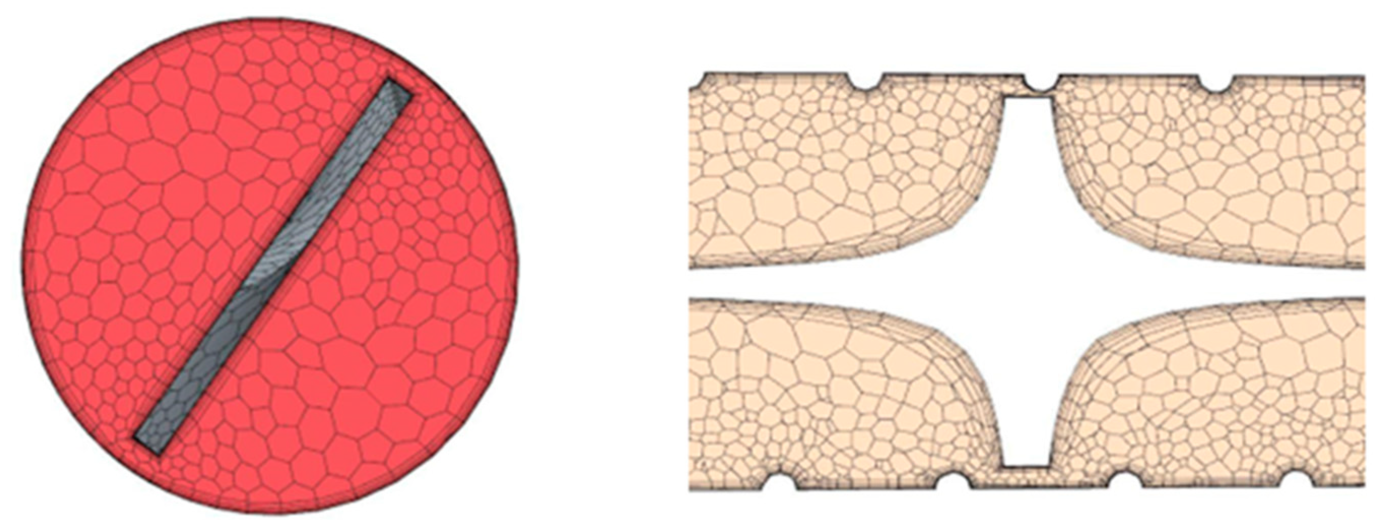
The geometry was modeled using SOLIDWORKS and then imported to STAR-CCM+ for simulation and analysis. A polyhedral mesh was used. Its main advantage is that each element has many adjacent cells, which helps reduce errors in gradients. Polyhedrons are also less susceptible to stretching than tetrahedrons, resulting in enhanced mesh quality and model numerical stability [6].

R1= 0.5s [1+0.25(t/s)2]-0.8

R2=0.5(e-s)[1+0.25(t/s)2]+0.8

A prism layer was also used to make the mesh finer at the walls of the tube and make the twisted tape capture the change of the temperature gradient. Figure 2 shows the prism layer with a total thickness of 10% of the mesh size. The mesh size is 3mm.It was found to be the best mesh supported by a grid independency study which will present later.

2.2. Governing Equations and Turbulence Model

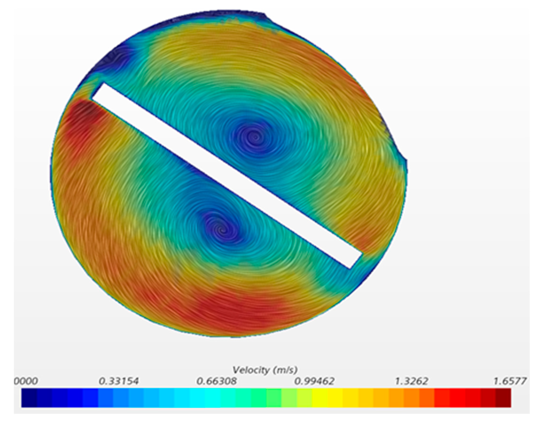
This study focuses on turbulent flow at a range of Reynolds number of 3.5 x 103 < Re < 5.0 x 104, and the twisted plate mixes the flow and adds turbulence as Figure 3 shows. The tubes are the same as the ones studied in Zimparov et.al (2012).

The governing equations of this simulation are the incompressible Reynolds averaged Navier-Stokes equations, the energy equation, and the steady 3-D form of the continuity [7].

Conservation of mass:

ρ \nabla \cdot \bar{V} = 0

(1)

Navier-Stokes equations:

ρ (\bar{u} \frac{\partial \bar{u}}{\partial x} + \bar{v} \frac{\partial \bar{u}}{\partial y} + \bar{w} \frac{\partial \bar{u}}{\partial z}) = ρ g_{x} - \frac{\partial \bar{p}}{\partial x} + μ [\frac{\partial^{} \bar{u' u'}}{{\partial x}^{}} + \frac{\partial^{} \bar{u' v'}}{{\partial y}^{}} + \frac{\partial^{} \bar{u' w'}}{{\partial z}^{}}] (x direction)

(2)

ρ (\bar{u} \frac{\partial \bar{v}}{\partial x} + \bar{v} \frac{\partial \bar{v}}{\partial y} + \bar{w} \frac{\partial \bar{v}}{\partial z}) = ρ g_{y} - \frac{\partial \bar{p}}{\partial y} + μ [\frac{\partial^{} \bar{v' u'}}{{\partial x}^{}} + \frac{\partial^{} \bar{v' v'}}{{\partial y}^{}} + \frac{\partial^{} \bar{v' w'}}{{\partial z}^{}}] (y direction)

(3)

ρ (\bar{u} \frac{\partial \bar{w}}{\partial x} + \bar{v} \frac{\partial \bar{w}}{\partial y} + \bar{w} \frac{\partial \bar{w}}{\partial z}) = ρ g_{z} - \frac{\partial \bar{p}}{\partial z} + μ [\frac{\partial^{} \bar{w' u'}}{{\partial x}^{}} + \frac{\partial^{} \bar{w' v'}}{{\partial y}^{}} + \frac{\partial^{} \bar{w' w'}}{{\partial z}^{}}] (z direction)

(4)

Conservation of Energy:

ρ c_{p} V . \nabla T = \nabla . k \nabla T + μ φ

(5)

Dissipation function:

φ = 2 [{(\frac{\partial u}{\partial x})}^{2} + {(\frac{\partial v}{\partial y})}^{2} + {(\frac{\partial w}{\partial z})}^{2}] + {(\frac{\partial u}{\partial y} + \frac{\partial v}{\partial x})}^{2} + {(\frac{\partial v}{\partial z} + \frac{\partial w}{\partial y})}^{2} + {(\frac{\partial w}{\partial x} + \frac{\partial u}{\partial z})}^{2}

(6)

The CFD model used is the k-ε model [1,8,9]. In the k–ε two equation model, the velocity and length scale of turbulence are defined with two additional partial-differential equations: one for the turbulent kinetic energy k, the other for the dissipation rate ε, and an algebraic demonstration for the eddy viscosity [1,8,9] is also given as in Eq. (9).

Kinetic energy Equation k:

ρ 〈u_{j}〉 \frac{\partial k}{{\partial x}_{j}} = 2 μ_{t} 〈s_{i j}〉 \frac{\partial 〈u_{i}〉}{{\partial x}_{j}} - ρ ε + \frac{\partial}{{\partial x}_{j}} ⌈(μ + \frac{μ_{t}}{σ_{k}}) \frac{\partial k}{{\partial x}_{j}}⌉

(7)

Dissipation rate equation ε:

ρ 〈u_{j}〉 \frac{\partial ε}{{\partial x}_{j}} = C_{ε 1} P_{k} \frac{ε}{k} - C_{ε 2} ρ \frac{ε^{2}}{k} + \frac{\partial}{{\partial x}_{j}} ⌈(μ + \frac{μ_{t}}{σ_{ε}}) \frac{\partial ε}{{\partial x}_{j}}⌉

(8)

Eddy Viscosity:

μ_{t} = C_{μ} ρ \frac{k^{2}}{ε}

(9)

The k and ε equations are solved with the mean Navier–Stokes equations. STAR-CCM+ offers a choice of eight different k–ε turbulence models. The constant variables of k–ε were suggested by STARCCM+ software as follows [1]: Cμ = 0.09, Cε1 = 1.44, Cε2 = 1.92, σk = 1.3 and σε = 1.

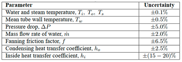
Table 2 provided by Zimparov et al. represents the errors of the measured parameters, which will be useful to validate the CFD model, as the goal is to check that the CFD results fall within those margins of errors. The CFD simulation will not be concerned by the steam temperature, as the wall temperature is enough to be used as a boundary condition.

2.3. Flow and Boundary Conditions

As mentioned earlier, the flow has a Reynolds number that ranges between 3.5 x 103 < Re < 5.0 x 104. The working fluid is water and the pipe walls are neglected, a temperature Tw is applied directly on the fluid according to Zimparov’s data.

The wall temperature ranged from 38 °C to 91.6 °C, the inlet temperature of the water ranged from 23.5 °C to 86.1 °C, and the inlet velocity of the water was calculated for each run from a given Re. A total of 16 runs were made for each tube. Table 3 and Table 4 show the boundary conditions for each experiment.

The water is considered incompressible, turbulent, three-dimensional, and at a steady state. A non-slip condition was considered for the walls, and the outlet pressure was the atmospheric pressure. The number of iterations needed to achieve convergence varied for each run as it got higher. As the Re number increased and the tube geometry changed, convergence ranged from 200 to 1500 iterations. Convergence was considered “achieved” when the energy equation residual reached 1E-4 and the flow was thermally fully developed.

2.4. Parameters and Metric Definitions

The three parameters of interest in investigating in this study are the Heat transfer coefficient and the friction factor. The inside heat transfer coefficient hi is represented as a function of Nu with the following relation:

N_{u} = \frac{h_{i} D ⅈ}{k}

(10)

While hi is:

h_{i} = \frac{\dot{Q}}{A_{i} Δ T_{m}}

(11)

Q ̇ is the heat transfer in (W) and it was an output from STAR-CCM+, then use Eq (11) to calculate hi.

Δ T_{m} = \frac{T_{0} - T_{i}}{l n (\frac{T w, m - T_{i}}{T w, m - T_{0}})}

(12)

The same equations (11,12,13) as Zimparov et.al [2] were used to maintain similarity. The accuracy of the temperature measurements was as follows: inlet and outlet water temperatures, steam temperature–0.1%, and mean tube wall temperature along the length –0.5%. The accuracy of the calculated heat transfer coefficients was estimated at 2.5% for the condensing heat transfer coefficient and at 15–20% for the inside heat transfer coefficient. All uncertainties of the measured quantities and calculated parameters are presented in Table 2 [1]. These uncertainties are used later to correlate between our CFD results and the experimental results.

The fanning friction factor is given by:

f = \frac{ρ π^{2} D ⅈ^5}{32 L} \frac{Δ P}{{\dot{m}}^{2}}

(13)

ΔP is the pressure drop. It was an output from STAR-CCM, then use Eq (13) to calculate f. Coefficient (η) is introduced to evaluate the gain in heat transfer against the energy loss due to the increased pressure drop caused by the tubes’ geometry (i.e., corrugations and twisted tape) [1].

η = \frac{\frac{N u}{N_{u s}}}{\frac{f}{f_{s}}}

(14)

Nu is the Nusselt number of a given tube and Nus is for the smooth tube. The same applies to the friction factor.

This ratios Nu/Nus and f/fs are a dimensionless representation of the heat transfer and friction factor, respectively, that allows for the comparison of both properties. Other papers have used a similar factor such as [13,14].

3. Results

3.1. Grid Independency Study

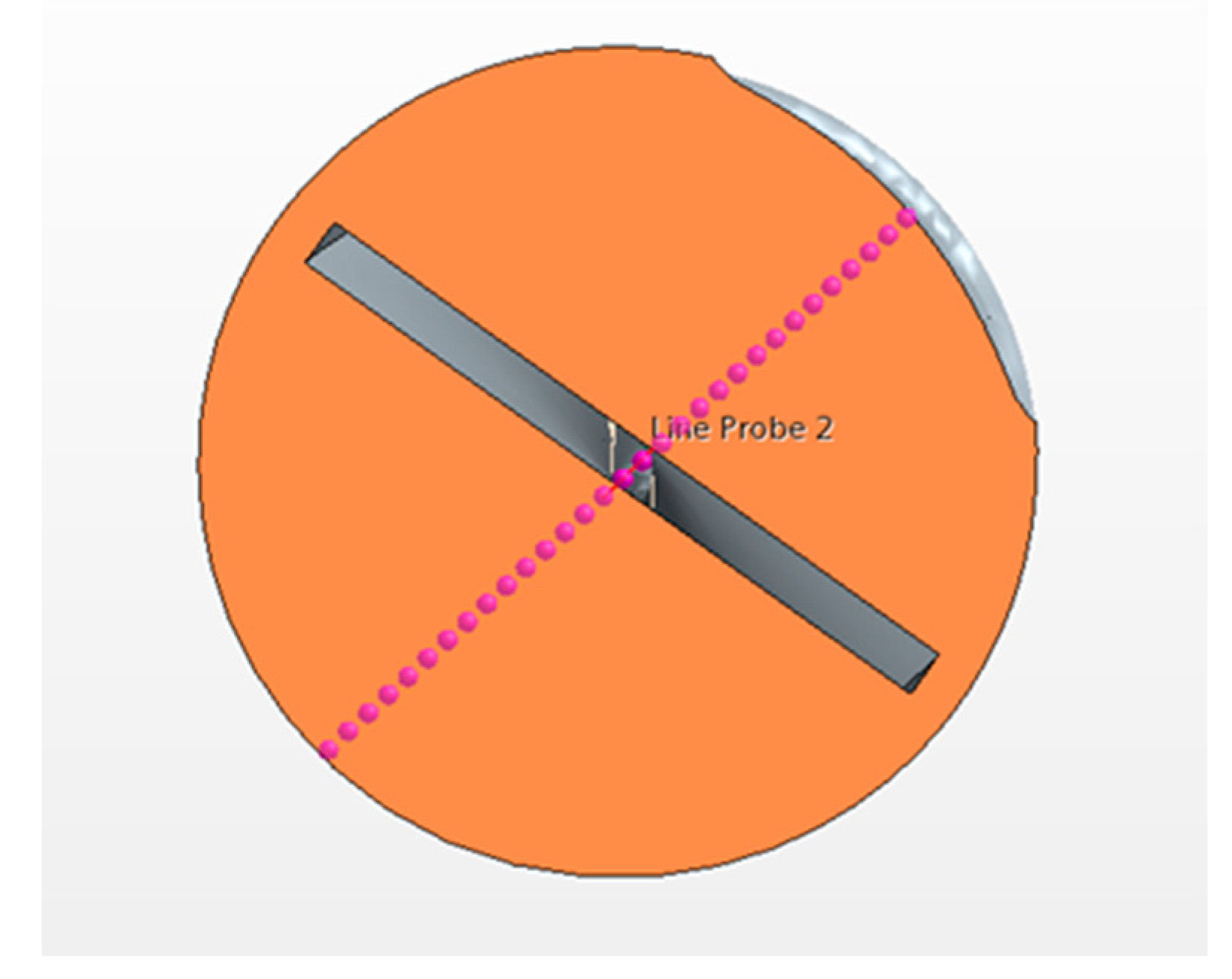
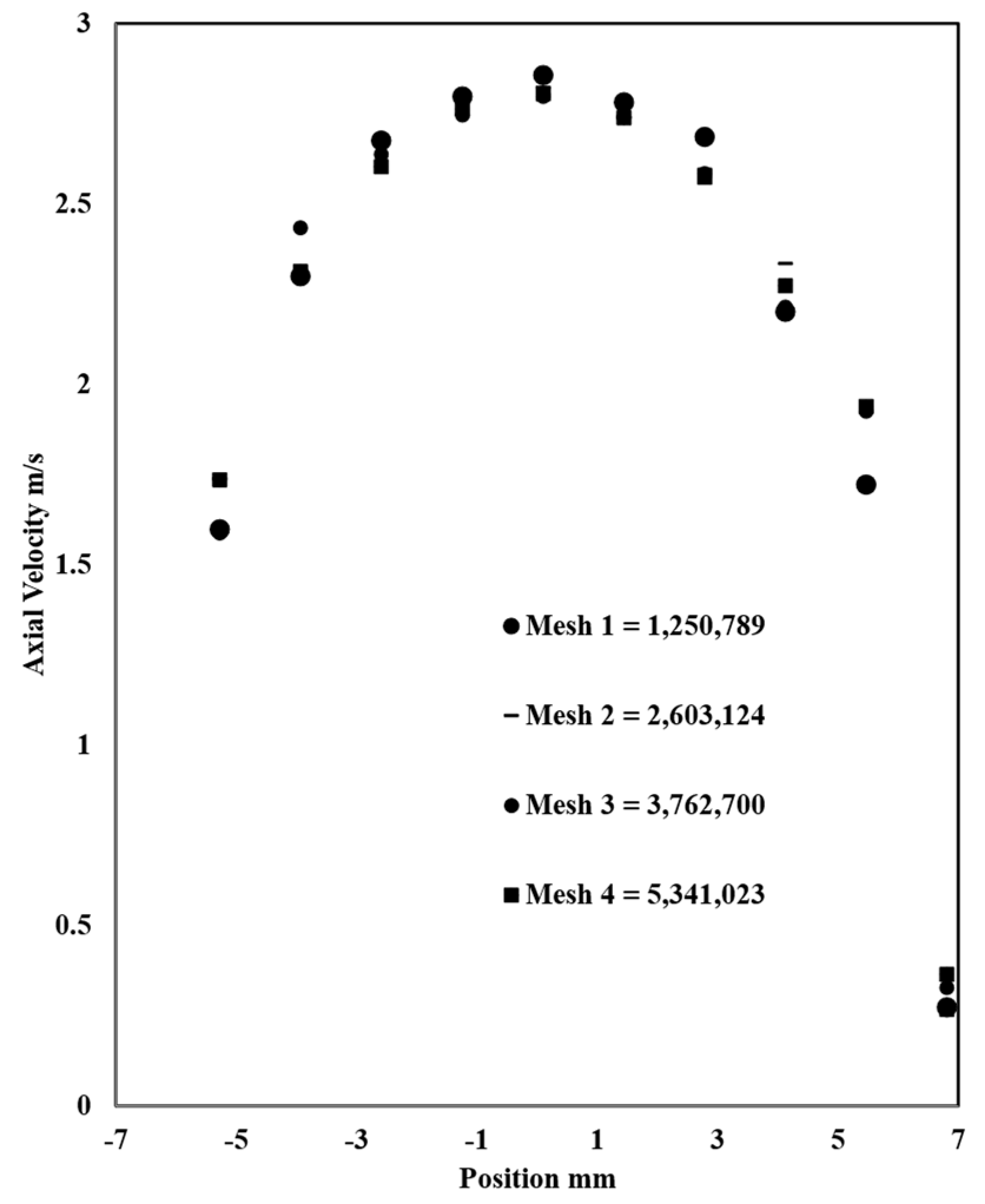
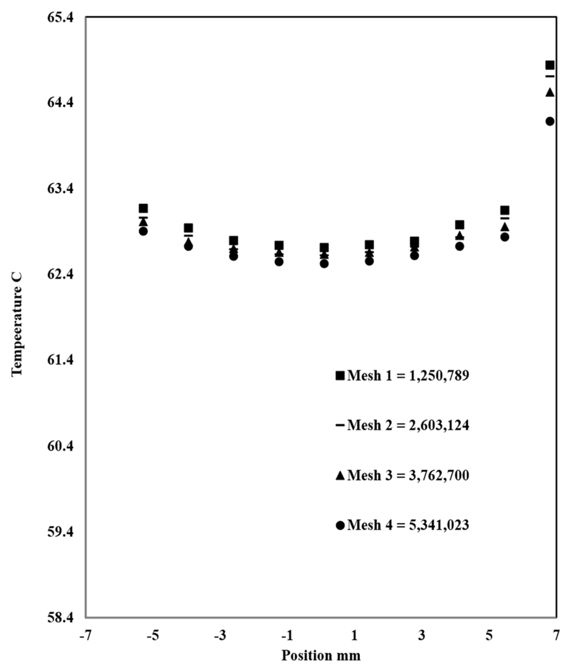
The grid independency study is done to achieve a 1–2% error between different mesh sizes, which will help to choose the right size that balances accuracy and computing time. Four grids were tested: grid 1: 1,250,789 elements; grid 2: 2,603,124 elements; grid 3: 3,762,700 elements; and grid 4: 5,341,023. The approach to choose the most optimal grid is done by comparing the heat transfer parameters; in this case, axial velocity and temperature along the outlet diameter for all the grids (Figure 4, Figure 5 and Figure 6). When the change in results becomes minimal as meshes becomes finer, then grid independency has been achieved and the grid with the smaller number of elements is chosen, after which the results do not change significantly. In this case, it is mesh 3.

3.2. Experimental Data and CFD Validation

To make sure the CFD model is correct, comparing the simulation results against experimental data [1] is necessary before conducting any further studies. The uncertainties from experimental measurement are represented by error bars (Table 2). The same boundary conditions from the experiment (Table 3 and Table 4) were used in the CFD simulation, courtesy of Dr. Zimparov. The Nusselt number, friction factor, and heat transfer coefficient were calculated from Eq 10, 11, and 13, while the pressure drop ΔP and heat transfer Q ̇ were obtained from the CFD results. In [1] the heat transfer coefficient was presented as Nu*Pr-0.4. The CFD validation is done by comparing key parameters (i.e., Heat Transfer coefficient, Friction factor and the Nusselt number). The purpose of this validation is to be able to use the same model parameters to confidently run other simulations with different geometries and expect reasonable accuracy.

Table 5 and Table 6 contain the experimental data obtained by Zimparov et al. (2012). This data will be compared to the CFD results to assess the numerical model’s accuracy.

3.3. Heat Transfer Coefficient

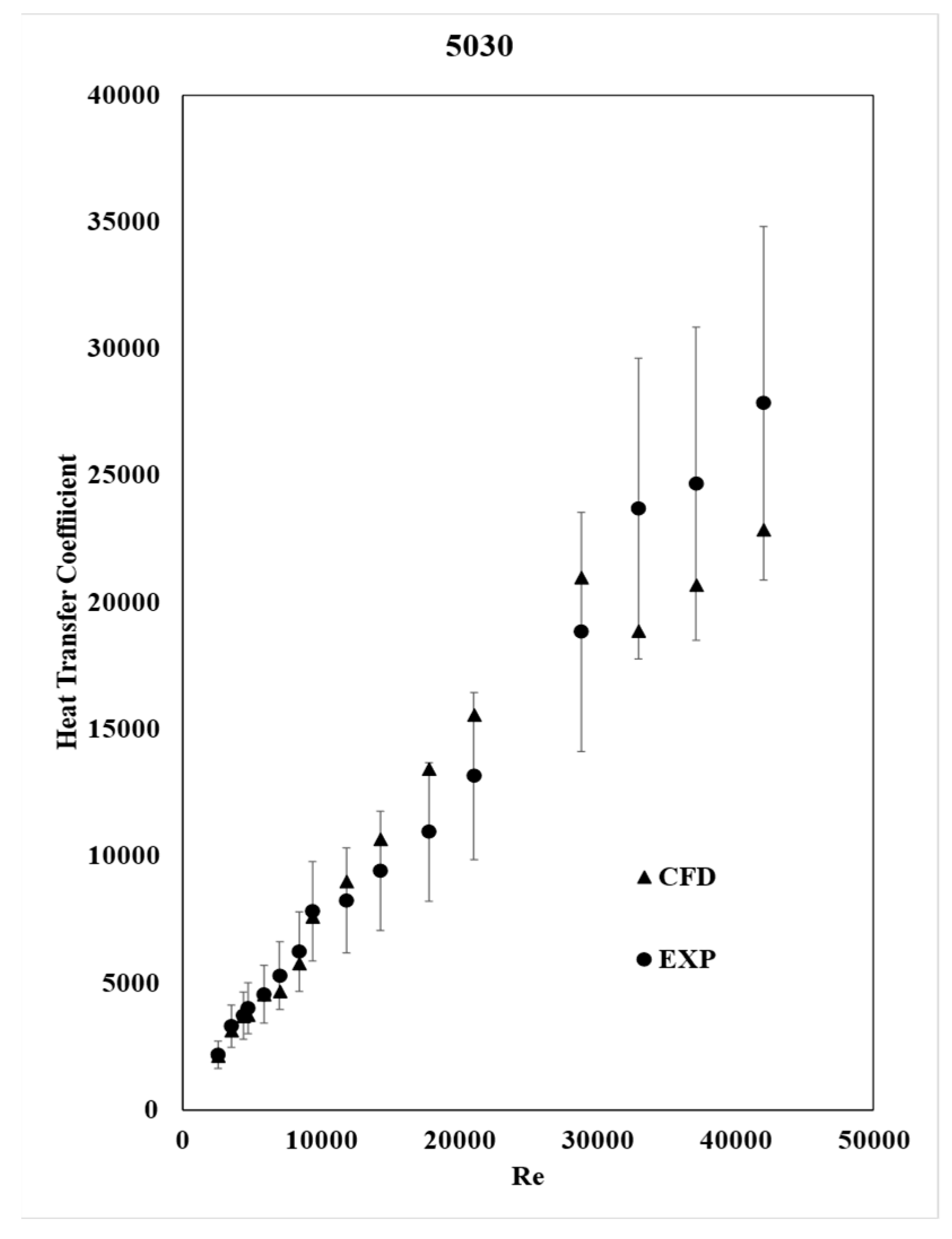
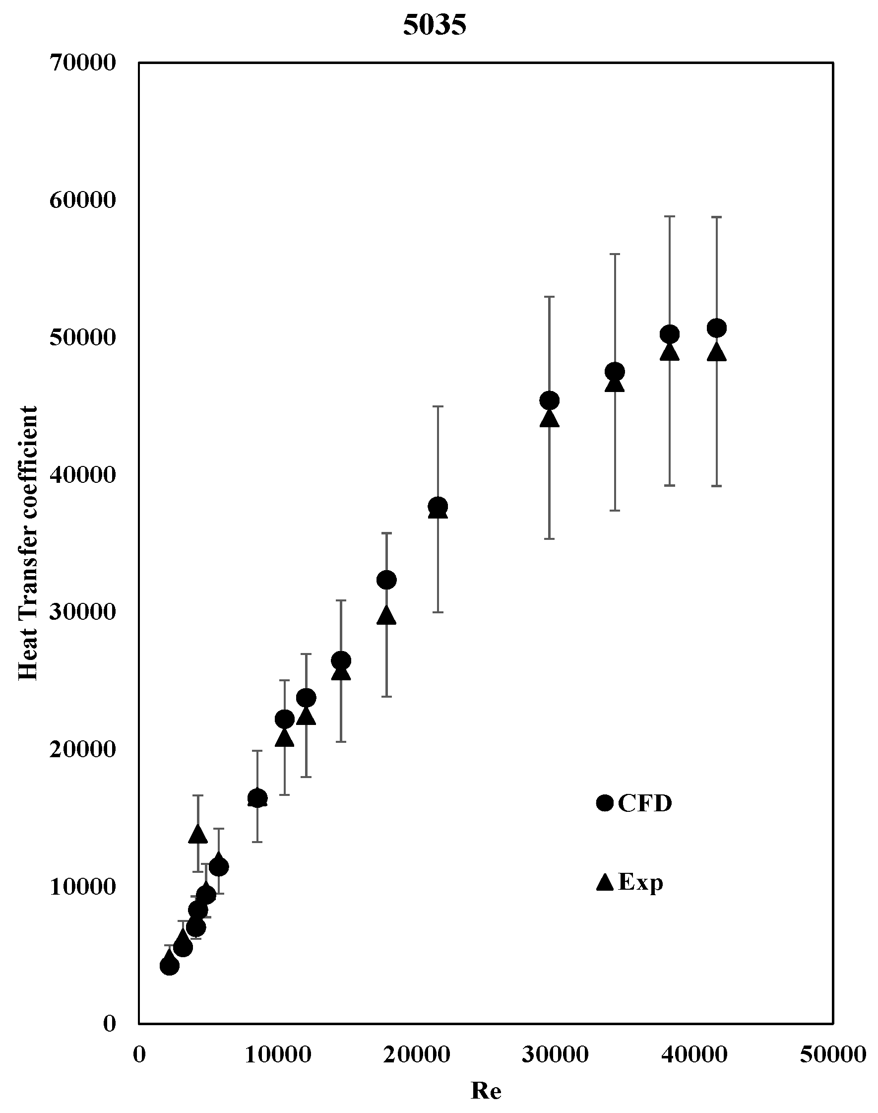
The heat transfer coefficient calculated is an average value on the inside walls of the tube. Figure 7 and Figure 8 show that the heat transfer coefficient increases with the Re number, and that the CFD results exhibit the same behavior as the experimental data.

The calculation was made by implementing equations 11 and 12 as a field function in STAR-CCM+, while the area and the heat transfer were calculated by the software automatically. As expected, the heat transfer is increased in tube 5035 due to the additional heat conduction provided by the plate insert.

The CFD results agree with the experimental ones and are within the error bars, indicating that the CFD model is accurate enough.

3.4. Friction Factor

The friction factor was also calculated by implementing equation 12 into the software, while the area, mass flow rate, and pressure drop were calculated automatically from STAR-CCM+.

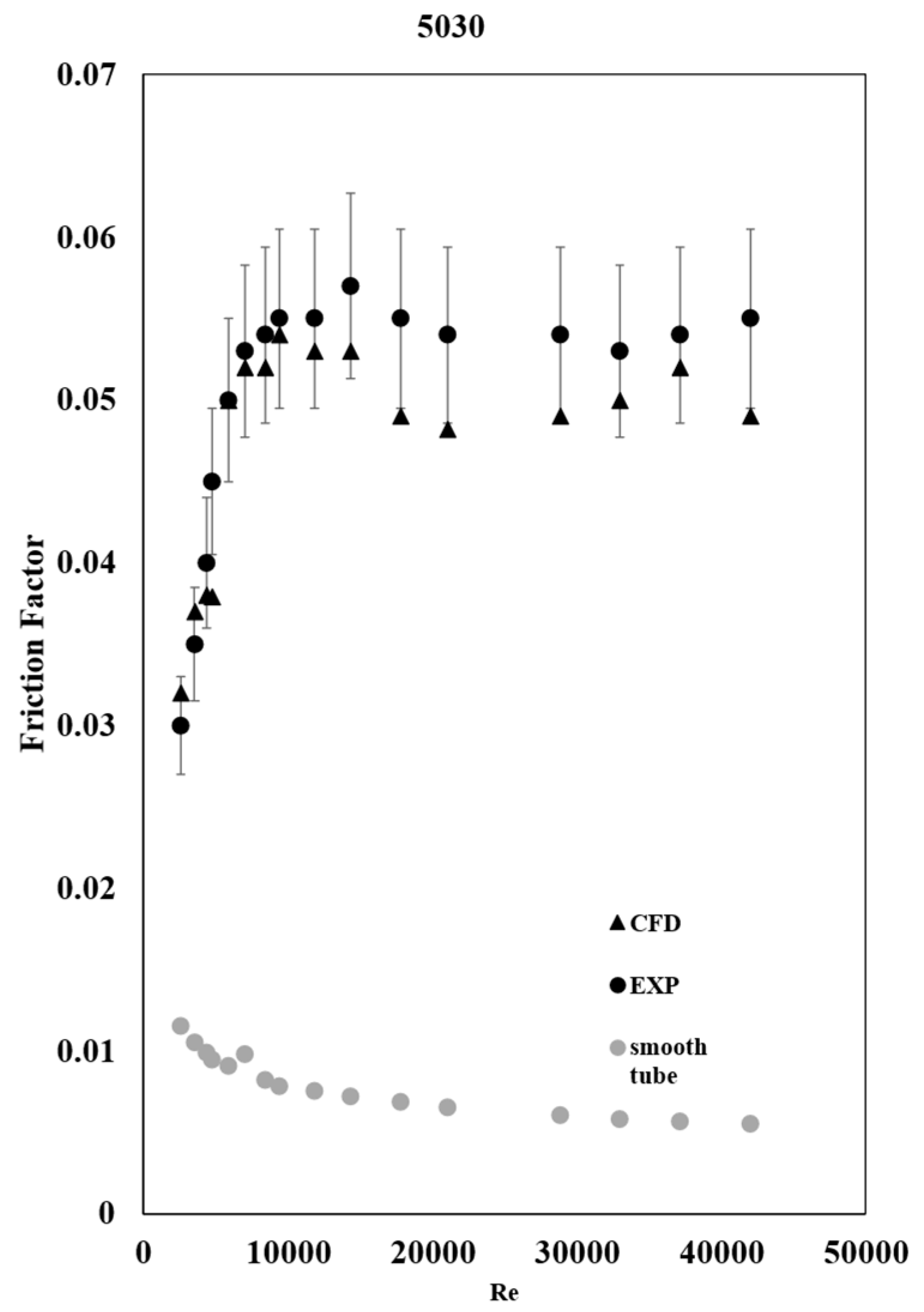
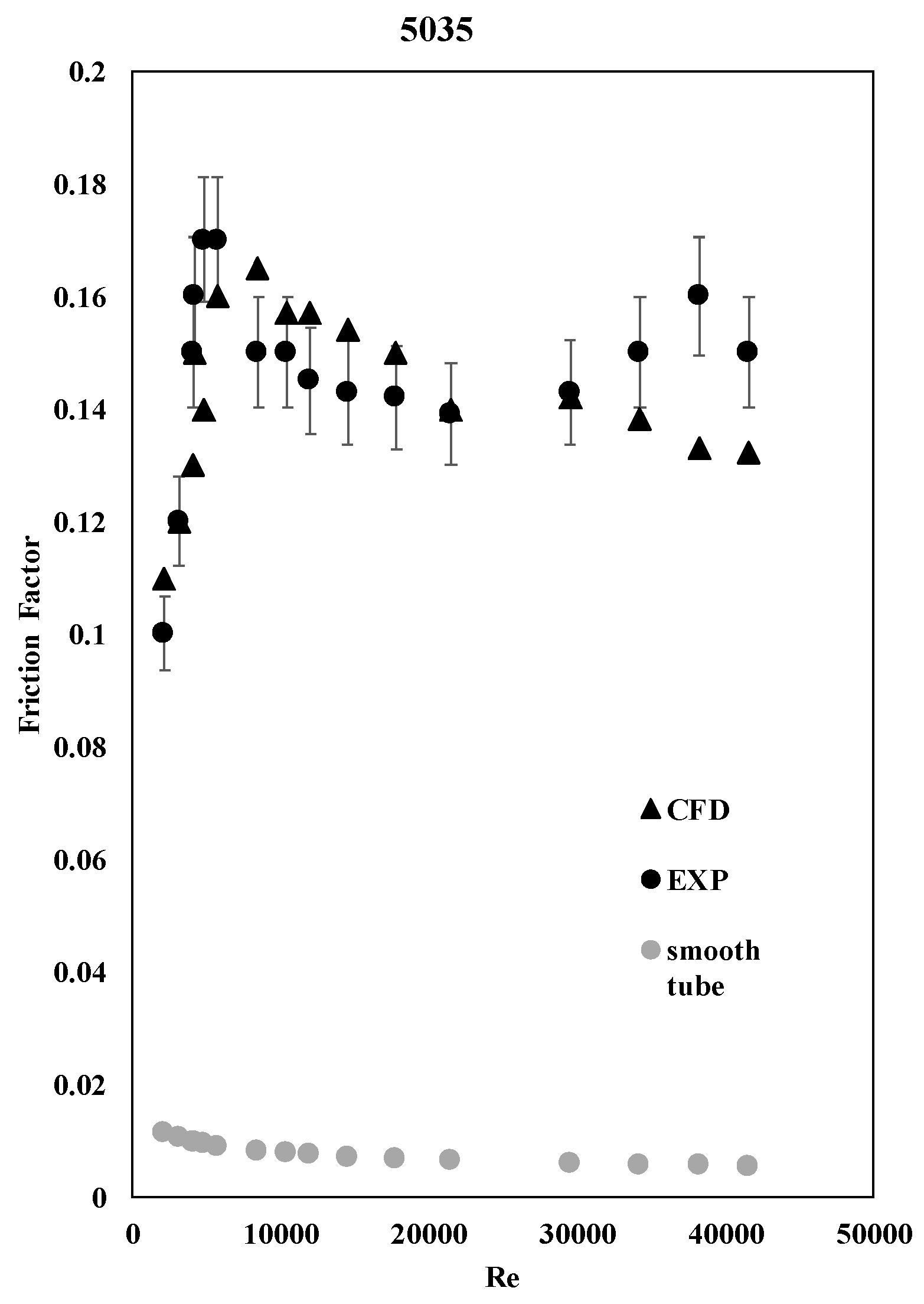
Here again, the CFD results agree with the experimental results as shown in Figure 9 and Figure 10 for tubes 5030 and 5035.

As expected, the friction factor increased substantially in tube 5035 due to the added friction by the twisted plate. This means that there is an increase in head loss, which will require more pumping power to get the water from one end to another.

3.5. Nusselt Number

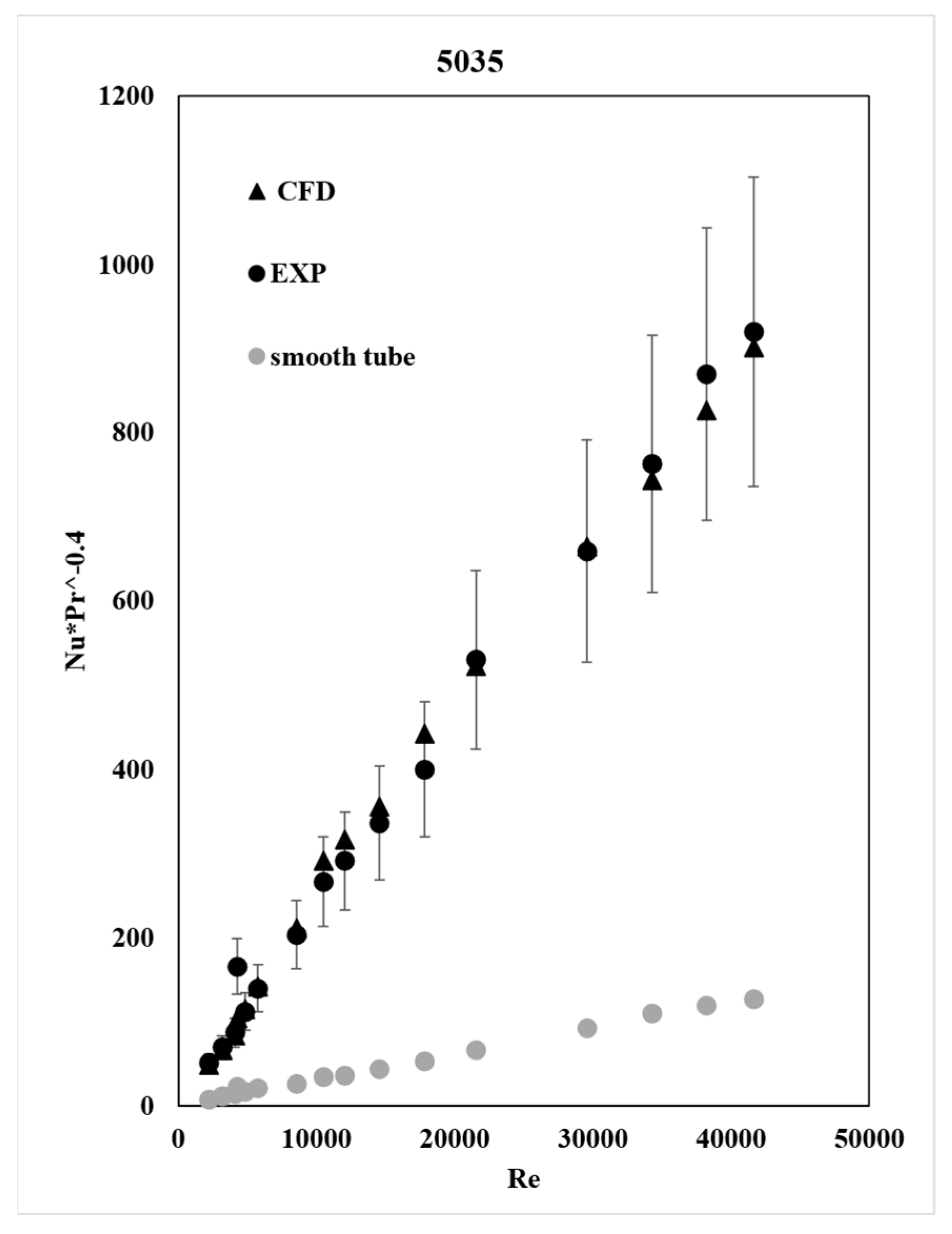
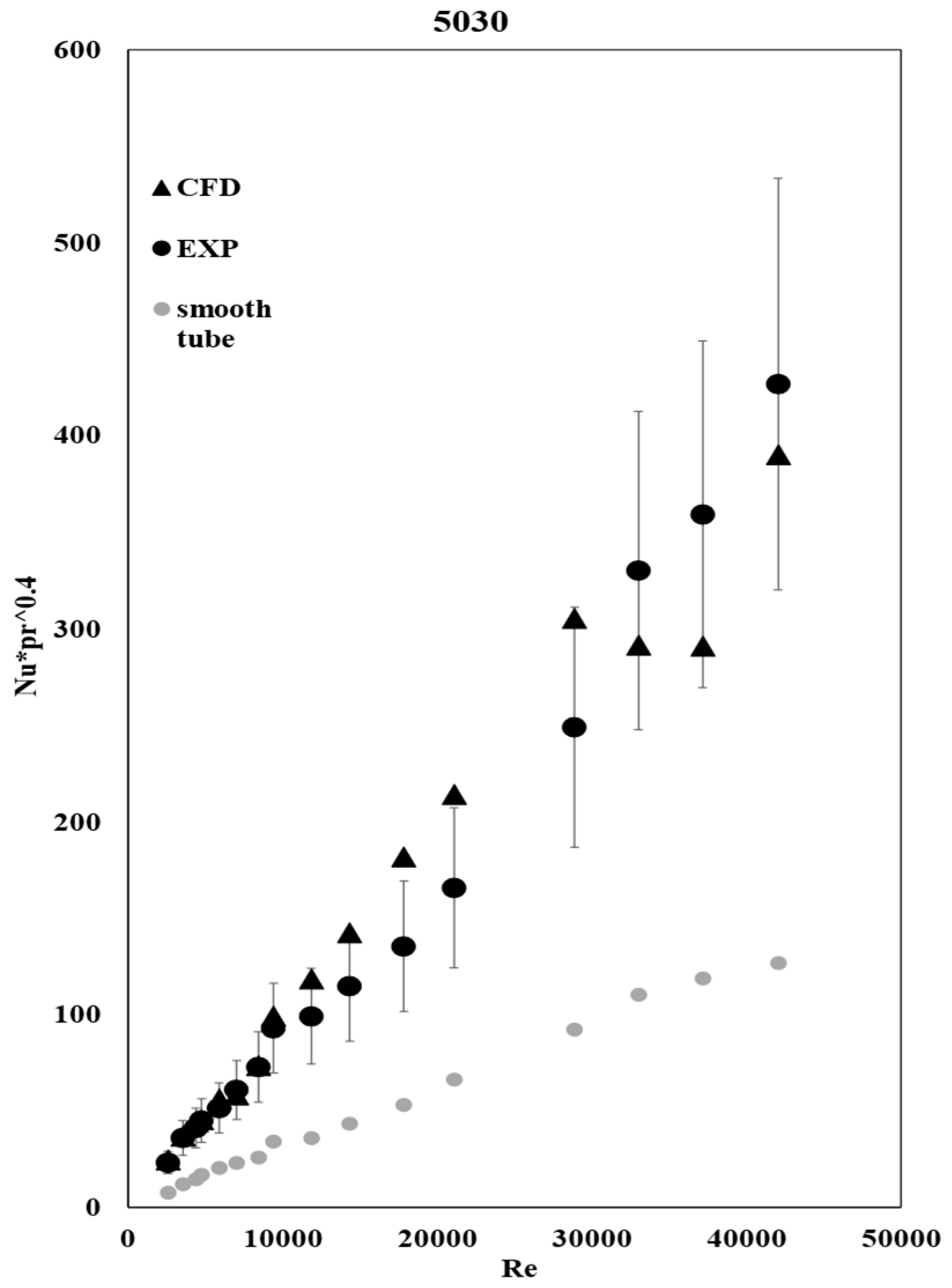
For both tubes 5030 and 5035, the Nusselt number kept increasing with Re as shown in Figure 11 and Figure 12. Zimparov et al. [2] represents the Nusselt number as NuPr-0.4, where Pr is the Prandtl number for water, and Nu is calculated using equation 10.

3.6. Turbulent Kinetic Energy

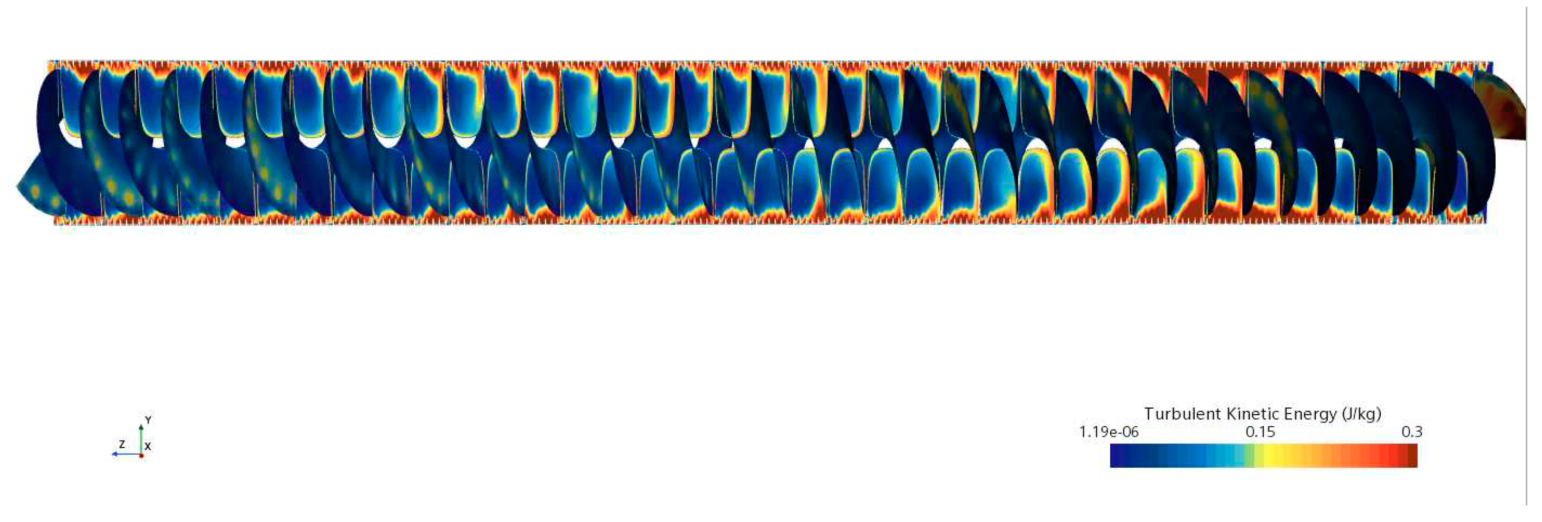
Figure 13 shows the turbulent kinetic energy on an axial plane through the tube’s axis and on the twisted tape’s walls. Figure 14 shows the Heat transfer coefficient on the wall of the tube.

A higher heat transfer coefficient is apparent in areas with high TKE. The turbulence introduced by the twisted tape promotes the heat transfer between the fluid and the wall. The CFD simulation proved useful in investigating the TKE, which could not have been done experimentally.

3.7. Thermal Performance

As mentioned in section 3.3, there was an increase in the amount of heat conducted by the twisted plate, but that comes with more friction caused by the plate’s geometry, which results in head loss as discussed in section 3.4.

Our goal is to increase the heat transfer without increasing the pressure drop to a level where it is no longer beneficial due to the required pumping power.

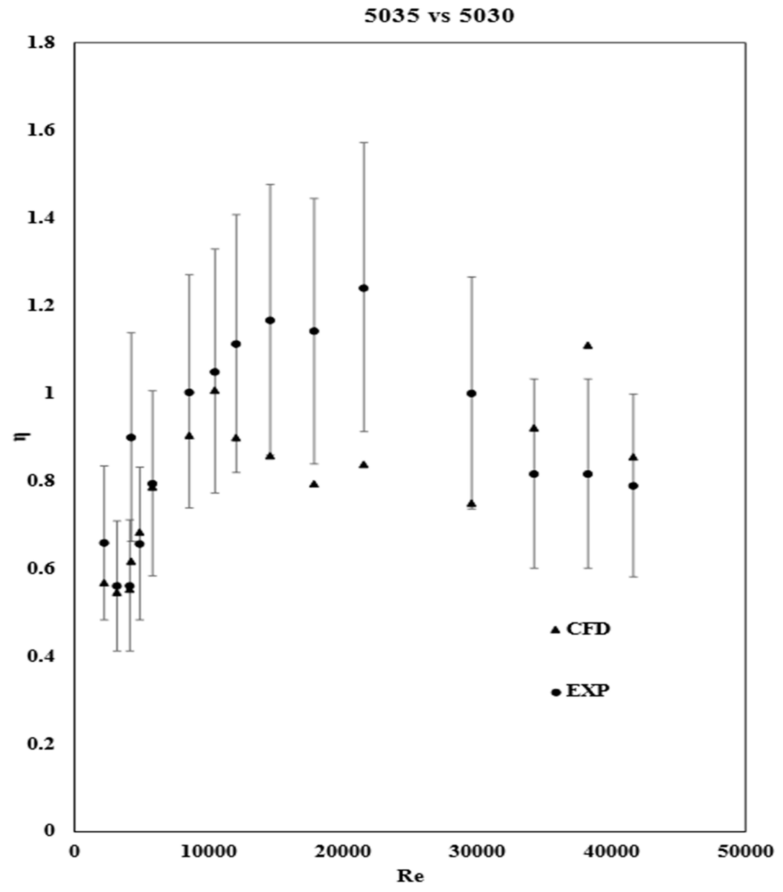
The enhancement factor (Eq.14) will allow us to evaluate the gain in heat transfer against the energy loss where Nu5/Nu0 is the ratio of the Nusselt number of tubes 5030 and 5035, and f5/f0 is the ratio for the fanning factor.

If η<1, that means that the friction factor is greater than the heat transfer, indicating that the tube’s design is not efficient for transferring heat without increasing the cost of energy consumption required for pumping.

On the other hand, if η ≥ 1, the tube design can be used for enhancement purposes.

The error bars represent the combined errors from the friction factor and the heat transfer coefficient, which is considered in the Nusselt number.

From Figure 15, the enhancement is beneficial when Re ranges from 10,000 to 28,000. Outside of this range, even though there is a greater heat transfer coefficient, the friction factor is high enough to require more energy to pump the water through the pipe, thus resulting in diminution of the η factor.

4. Conclusions

The enhancement in heat transfer is undeniable in tubes with a twisted insert, but according to this study’s CFD results, when the friction caused by the twisted plate is considered, the enhancement is optimal only for Re ranging from 10,000 to 28,000, where 39.6C< Ti <51.5C and 49.3C<Tw<91.8C. For higher Re, the Nusselt number increased significantly due to the elevated turbulence, and thus, an increased mixing of the flow in the transverse direction but with higher friction it requires more power to pump the flow.

The CFD model accurately predicted the experimental data, and the parameters used in the model are appropriate and can be replicated in similar simulations.

Figure 7 and Figure 8 show that the compound enhancement method has an undeniable positive effect on the heat transfer coefficient. Tube 5035 with both corrugations and the twisted insert had a heat transfer coefficient 2 to 3 times higher than tube 5030 with only corrugations at the same Re number range. A practical use of such heat exchangers can be in nuclear reactor cooling, automotive radiators, and other applications where tubular heat exchangers are used.

On the other hand, the pressure drop increased significantly as well. Figure 9 and Figure 10 show that tube 5035 experienced more than 2 times the pressure drop when compared to tube 5030 at the same Re number range.

For future research, the authors are planning to try a different geometry for the insert, which will hopefully perform better by decreasing the pressure drop while maintaining a high enough heat transfer coefficient.

References

S. Pirbastami, S.F. Moujaes, S.G. Mol Computational fluid dynamics simulation of heat enhancement in internally helical grooved tubes Int. Commun. Heat Mass Transf., 73 (2016), pp. 25-32,. [CrossRef]
Zimparov, Ventsislav & Petkov, Valentin & Bergles, Arthur. (2012). Performance characteristics of deep corrugated tubes with twisted-tape inserts. Journal of Enhanced Heat Transfer. 19. 1-11. [CrossRef]
P.G. Vicente, A. Garcıa Viedma, A. Experimental investigation on heat transfer and frictional characteristics of spirally corrugated tubes in turbulent flow at different Prandtl numbers Int. J. Heat Mass Transf., 47 (4) (2004), pp. 671-681. [CrossRef]
E.M. Sparrow, A.T. PrataNumerical solutions for laminar flow and heat transfer in a periodically converging-diverging tube, with experimental confirmation Numerical Heat Transfer, 6 (4) (1983), pp. 441-461. [CrossRef]
Peng Yang, Hongwei Zhang, Yongyu Zheng, Zhenjian Fang, Xueli Shi, Yingwen Liu, Investigation and optimization of heat transfer performance of a spirally corrugated tube using the Taguchi method,International Communications in Heat and Mass Transfer,Volume 127,2021,105577, ISSN 0735-1933,. [CrossRef]
Sosnowski, Marcin; Krzywanski, Jaroslaw; Grabowska, Karolina; Gnatowska, Renata. Polyhedral meshing in numerical analysis of conjugate heat transfer EPJ Web of Conferences; Les Ulis, Vol. 180, (2018). [CrossRef]
L.M. Jiji, Heat Convection, second ed. Springer, Germany, 2006 22–45.
STAR-CCM+ user manual, version 9.04.009. CD-Adapco, 2013.
O. Zikanov, Essential Computational Fluid Dynamics, first ed. Wiley, New York, 2010.
K. Ceylan, G. Kelbaliyev, The roughness effects on friction and heat transfer in the fully developed turbulent flow in pipes, Appl. Therm. Eng. 23 (2003) 557–570. [CrossRef]
Rahimi, M., Shabanian, S.R., Alsairafi, A.A., 2009. Experimental and CFD studies on heat transfer and friction factor characteristics of a tube equipped with modified twisted tape inserts. Chem. Eng. Process. Process Intensif. 48, 762–770. [CrossRef]
Lou, J.Z., Li, J.P., Dong, Y.J., Wang, M., 2011. Study on Simulation of Heat Transfer Tubes with Twisted-Tape Inserted. Appl. Mech. Mater. 66–68, 1342. [CrossRef]
Shaver, D.R., Carasik, L.B., Merzari, E., Salpeter, N., Blandford, E., 2019. Calculation of Friction Factors and Nusselt Numbers for Twisted Elliptical Tube Heat Exchangers Using Nek5000. J. Fluids Eng. Trans. ASME. [CrossRef]
Wu, C.-C., Chen, C.-K., Yang, Y.-T., Huang, K.-H., 2018. Numerical simulation of turbulent flow forced convection in a twisted elliptical tube. Int. J. Therm. Sci. 132, 199–208. [CrossRef]

Figure 1. (a,b). Pictures showing the geometrical parameters presented in Table 1 [2].

Figure 2. Volume mesh showing prism layer at the solid boundaries.

Figure 3. Scalar scene showing swirls created by the twisted plate.

Figure 4. Probe line along the outlet diameter for axial velocity and temperature results.

Figure 5. Axial velocity for four different meshes along the outlet diameter of the pipe.

Figure 6. Axial temperature for four different meshes along the outlet diameter of the pipe.

Figure 7. Comparison of Heat Transfer factor obtained from CFD simulation with experimental data [2] for tube 5030.

Figure 8. Comparison of Heat Transfer factor obtained from CFD simulation with experimental data [2] for tube 5035.

Figure 9. Comparison of friction factor obtained from CFD simulation with experimental data [2] for tube 5030.

Figure 10. Comparison of friction factor obtained from CFD simulation with experimental data [2] for tube 5035.

Figure 11. Comparison of Nusselt Number obtained from CFD simulation with experimental data [2] for tube 5035 and smooth tube.

Figure 12. Comparison of Nusselt number obtained from CFD simulation with experimental data [2] for tube 5030 and smooth tube.

Figure 13. Turbulent kinetic energy plot for tube 5035.

Figure 14. Heat Transfer coefficient plot for tube 5035.

Figure 15. Enhancement factor η comparing the performance of tube 5035 with 5030.

Table 1. Geometric parameters of tube 5030.

No	D_o mm	D_i mm	e mm	p mm	β deg	t mm	s mm	e/D_i	p/e	Β_*	Twisted tape
5030	15.31	13.51	0.767	5.19	83.0	1.836	0.371	0.057	6.77	0.922	N/A
5035	15.31	13.51	0.767	5.19	83.0	1.836	0.371	0.057	6.77	0.922	H/Di=4.7

Table 2. Uncertainties of measured and calculated parameters [2].

Table 3. Boundary Conditions for 5030 [2].

Run	Re	Vi (m/s)	Ti (C)	Tw (C)
1	2590	0.170482	26	43.1
2	3540	0.233013	28.4	43.4
3	4400	0.289621	30.9	43.3
4	4750	0.312659	32.6	44
5	5900	0.388356	34.8	45.4
6	7030	0.462736	36.5	45.9
7	8440	0.555546	38.6	49.3
8	9420	0.620053	40.8	52
9	11860	0.780661	43	52.7
10	14340	0.943902	45.4	53.8
11	17840	1.174283	47.9	54.9
12	21090	1.388207	50.4	56.5
13	28870	1.90031	58.4	64
14	33010	2.172818	67	74.4
15	37170	2.446641	76.4	83.6
16	42060	2.768516	86	91.6

Table 4. Boundary Conditions for 5035 [2].

Run	Re	Vi (m/s)	Ti (C)	Tw (C)
1	2220	0.146111	23.5	38
2	3180	0.209294	27.7	41
3	4110	0.270502	30	41.4
4	4850	0.319206	32.8	43.2
5	5760	0.379098	35	44.1
6	4260	0.280375	37.3	45
7	8540	0.562066	39.6	47.55
8	10500	0.691064	42.1	50.9
9	12050	0.793079	44.4	52.1
10	14560	0.958276	46.4	52.8
11	17840	1.174151	48.8	55.1
12	21540	1.417669	51.1	56.95
13	29570	1.946169	60.1	63.5
14	34280	2.256161	69.5	76.05
15	38240	2.516791	78.5	84.62
16	41620	2.739248	86.1	91.8

Table 5. Experimental results for 5035 [2].

5035
No	Re	pr	NuPr*-0.4	h W/(m².K)
1	2220	5.41	51.2	4760
2	3180	4.96	69.5	6240
3	4110	4.81	87.1	7730
4	4850	4.55	111.9	9700
5	5760	4.4	139.7	11850
6	4260	4.27	165.6	13850
7	8540	4.07	203.4	16550
8	10500	3.85	266.5	20840
9	12050	3.72	291	22440
10	14560	3.63	336.1	25690
11	17840	3.48	399.7	29770
12	21540	3.35	530.1	37470
13	29570	2.93	659.1	44130
14	34280	2.48	763.1	46710
15	38240	2.19	869.4	49000
16	41620	1.99	919.5	48960

Table 6. Experimental results for 5030 [2].

5030
No	Re	pr	NuPr*-0.4	h W/(m².K)
1	2220	5.22	23.3	2170
2	3180	4.96	36.1	3310
3	4110	4.81	41.3	3730
4	4850	4.66	45.1	4020
5	5760	4.48	51.6	4560
6	4260	4.35	60.9	5300
7	8540	4.15	72.9	6250
8	10500	3.93	93	7830
9	12050	3.83	99.1	8260
10	14560	3.7	114.8	9420
11	17840	3.57	135.4	10960
12	21540	3.43	165.7	13170
13	29570	2.98	248.8	18850
14	34280	2.57	330	23710
15	38240	3.25	359.2	24690
16	41620	2	426.6	27860

Disclaimer/Publisher’s Note: The statements, opinions and data contained in all publications are solely those of the individual author(s) and contributor(s) and not of MDPI and/or the editor(s). MDPI and/or the editor(s) disclaim responsibility for any injury to people or property resulting from any ideas, methods, instructions or products referred to in the content.

© 2023 by the authors. Licensee MDPI, Basel, Switzerland. This article is an open access article distributed under the terms and conditions of the Creative Commons Attribution (CC BY) license (http://creativecommons.org/licenses/by/4.0/).

Copyright: This open access article is published under a Creative Commons CC BY 4.0 license, which permit the free download, distribution, and reuse, provided that the author and preprint are cited in any reuse.

MDPI Initiatives

Important Links

Choose an area of interest and we will send you notifications of new preprints at your preferred frequency.

Disclaimer

CFD Analysis of Heat Transfer Enhancement for Twisted Tape Inserted in spirally Corrugated Tubes

Abstract

1. Introduction

2. Numerical Method and Procedure

2.1. Geometry and Grid Generation

2.2. Governing Equations and Turbulence Model

2.3. Flow and Boundary Conditions

2.4. Parameters and Metric Definitions

3. Results

3.1. Grid Independency Study

3.2. Experimental Data and CFD Validation

3.3. Heat Transfer Coefficient

3.4. Friction Factor

3.5. Nusselt Number

3.6. Turbulent Kinetic Energy

3.7. Thermal Performance

4. Conclusions

References

MDPI Initiatives

Important Links

Subscribe