Preprint
Article

PEIPNet: Parametric Efficient Image-Inpainting Network with Depthwise and Pointwise Convolution

Altmetrics

Downloads

92

Views

40

Comments

0

A peer-reviewed article of this preprint also exists.

This version is not peer-reviewed

Submitted:

31 August 2023

Posted:

05 September 2023

You are already at the latest version

Alerts
Abstract
Research on image-inpainting tasks has mainly focused on enhancing performance by augmenting various stages and modules. However, this trend does not consider the increase in the number of model parameters and operational memory, which increases the burden on computational resources. To solve this problem, we propose a Parametric Efficient Image InPainting Network (PEIPNet) for efficient and effective image-inpainting. Unlike other state-of-the-art methods, the proposed model has a one-stage inpainting framework in which depthwise and pointwise convolutions are adopted to reduce the number of parameters and computational costs. To generate semantically appealing results, we selected three unique components: spatially-adaptive denormalization (SPADE), dense dilated convolution module (DDCM), and efficient self-attention (ESA). The SPADE was adopted to conditionally normalize activations according to the mask to distinguish between damaged and undamaged regions. The DDCM was employed at every scale to overcome the gradient-vanishing obstacle and gradually fill-in pixels by capturing global information along the feature maps. The ESA was utilized to obtain clues from unmasked areas by extracting long-range information. In terms of efficiency, our model has the lowest operational memory compared with other state-of-the-art methods. Both qualitative and quantitative experiments demonstrate the generalized inpainting of our method on three public datasets: Paris StreetView, CelebA, and Places2.
Keywords: 
Subject: Computer Science and Mathematics  -   Artificial Intelligence and Machine Learning

1. Introduction

Image inpainting attempts to generate masked regions with visually satisfying image structures and regional features. This task has long been a major research area in computer vision. However, rapid changes have occurred in recent years with the emergence of deep learning. For example, traditional methods [1,2,3,4,5,6,7,8,9] only used known pixels for weighted replication or diffusion. However, deep learning-based approaches [10,11,12,13,14,15,16,17,18] continuously compress masked images into a dense latent space and fill-in the missing pixels by restoring high-level semantic information. The strength of deep learning-based methods is clearly demonstrated in large-hole inpainting tasks.
Various deep learning-based models have been introduced with the development of convolutional neural networks (CNNs) and generative adversarial networks (GANs) [19]. For instance, in accordance with the traditional concept, the methods [16,17,20,21,22] integrate a patch-matching algorithm into the latent space to effectively generate pixels and produce results that are visually pleasing. To address the limitations of vanilla convolution, partial convolution (PConv) and gated convolution (GConv) were proposed in [13,23], in which valid pixels were conditioned by the mask that acted as a prior. The framework of inpainting models also plays a key role in performance enhancement. Specifically, the methods [24,25,26,27] adopted a two-stage inpainting architecture in which the overall structural features of the masked regions were forecast in the first stage, while the final result was predicted in the second stage by adopting the output of the previous step as a constraint. Typically, the Edge Connect (EC) [24] recovers the missing edges in the first stage by piling up numerous residual blocks with dilated convolutional layers, which increases the receptive field of the model and extracts global features. In the second stage, the restored edge map is employed in texture synthesis and ensures the visual unity of the final result. However, these approaches often require separate training, in which the end-to-end training strategy cannot be applied and increases the training complexity. Moreover, because two distinct models are employed to form a generator, the number of parameters and model complexity also increase as the probability of having an overfitting problem increases. This increases the usage of the operational memory, which hinders the use of inpainting models on restricted computational resources.
To solve these problems, we proposed the Parametric Efficient Image InPainting Network (PEIPNet) with a one-stage inpainting framework. First, we adopted depthwise and pointwise convolutions instead of the vanilla convolution to minimize the number of model parameters, which was inspired by [28]. Second, we employed spatially-adaptive denormalization (SPADE) [29] to conditionally normalize the feature maps according to the mask. Third, we introduced a dense dilated convolution module (DDCM), inspired by [30], to gradually fill-in the missing regions at different scales and mitigate the gradient-vanishing problem. Finally, efficient self-attention (ESA) [31] was utilized to capture long-range information from unmasked areas to enhance the inpainting accuracy.
To the best of our knowledge, the proposed PEIPNet is the first method in the image-inpainting task that has less than one million model parameters but ensures high performance. The contributions of this study are summarized as follows:
  • An efficient one-stage inpainting framework with effective modules is proposed to reduce the number of model parameters and computational costs to mitigate the overfitting problem when trained on small datasets, with potential applications in various environments.
  • Qualitative and quantitative evaluations conducted on different public datasets demonstrate the excellent performance of our method compared with state-of-the-art models.

2. Related Works

2.1. Image Inpainting by Patch-Based Methods

Patch-based methods were first introduced for texture synthesis [1,3], and then adopted in [32] for image inpainting to fill-in masked areas at the image level. These approaches normally inspect and copy comparable patches from a database or uncontaminated background into missing regions according to the distance metrics between different patches, i.e., Euclidean distance and SIFT distance [33]. Bertalmio et al. [4] merged patch-based texture combination techniques with diffusion-based dispersion under image decomposition. PatchMatch [9] was proposed to search for similar matches between image patches. Therefore, patch-based designs for image inpainting can produce sharp outputs with similar contexts. However, generating semantically plausible images by a patch-based approach remains difficult because a high-level understanding of the images is required.

2.2. Image Inpainting by Deep Generative Methods

Generative models based on neural networks for image inpainting typically encode a damaged image into a latent feature. In the latent space, the masked areas are filled-in at the feature level, and the feature maps are decoded and restored into an image. In recent years, studies based on deep generative models have yielded promising results. The Context Encoder (CE) [10] is one of the first neural networks that adopted deep feature learning and adversarial training [19]. The CE can generate visually appealing outputs for semantic hole-filling. In terms of the loss function, a guidance loss was proposed in [16], which forced the feature maps produced in the decoder to become similar to those of the ground-truth images made in the encoder. The methods in [11,24] employed dilated convolution to increase the receptive field of the model and capture global features. A two-stage inpainting framework was utilized in [24,25,26,27] to fill-in the pixels with the constraints generated in the first stage. Instead of vanilla convolution, PConv [14] and GConv [23] were designed to eliminate the effects that are induced by placeholder values in the masked areas of an image. A contextual attention (CA) layer [18] was proposed to fill-in the lost pixels with similar patches from undistorted areas in high-level feature maps. With regard to the CA layer, Sagong et al. [21] introduced a novel parallel extended-decoder path with a modified CA module to reduce the computational cost. However, minimizing the capacity of the model to increase its efficiency and solve the overfitting problem remains a challenge.

2.3. Conditional Normalization

A normalization layer for feature extraction is commonly applied in deep neural networks to aid the training process.
For instance, batch normalization (BN) [34] normalizes the activation maps across batch and spatial dimensions that affect generative networks. Instance normalization (IN) [35] differs from BN because it normalizes the features only across spatial dimensions and enhances the outcomes of numerous generative tasks, such as style transformation. Layer normalization (LN) [36] normalizes activations across the channel and spatial dimensions, and helps train recurrent neural networks more stably. Group normalization (GN) [37] normalizes the features of grouped channels of an instance, which boosts the performance of specific vision tasks such as object detection.
Conditional normalization differs from a single set of affine parameters in the aforementioned normalization approaches. Conditional normalization methods typically utilize external information to learn multiple sets of affine parameters. Conditional IN [38], adaptive IN [39], conditional BN [40], and SPADE [29] were introduced in image synthesis tasks. In the image-inpainting task, region normalization (RN) [41] was introduced for spatial region-wise normalization to overcome the limitations of typical feature normalization methods without considering the impact of the corrupted areas of the input image during the normalization process.

2.4. Neural Networks with Lightweight Architecture

Lightweight neural networks have been introduced to allow model developers to select a small network that corresponds to resource restrictions, i.e., latency and size. In particular, many studies have been conducted on image classification tasks to reduce the model capacity. Depthwise separable convolution was adopted in [42] and MobileNets [28] to reduce the computations in the first few layers. In contrast, flattened networks [43] construct a network with fully factorized convolution and demonstrate the effectiveness of intensely factored models. Factorized convolution was employed in factorized networks [44] similar to that in topological conjunctions. Afterwards, Xception [45] scaled-up the depthwise separable convolution to exceed the performance of Inception-V3 [46]. SqueezeNet [47] is another remarkably small network that uses a bottleneck method to reduce the number of required parameters. Structured transform networks [48] and deep fried convnets [49] were proposed to reduce computational costs. However, none of these strategies have been applied in image-inpainting tasks to scale down the model capacity.

3. Methodology

In this section, we first introduce the architecture of the proposed method and then explain the various loss functions used for training.

3.1. Generator Architecture

Figure 1 shows the architecture of the proposed method, which employs an autoencoder framework. To minimize the number of model parameters, we introduced a combination of depthwise and pointwise convolutions, as in [28]. Depthwise and pointwise convolutions were employed sequentially at the encoder, and applied in the opposite order at the decoder. In both parts, depthwise convolutions with a kernel size of 3 × 3 were used to extract features and increase the receptive field. Pointwise convolutions with a kernel size of 1 × 1 were used to alter the number of channels. For all convolutional modules, spectral normalization [50] was used to stabilize the training process. SPADE [29] was chosen to conditionally normalize the masked and unmasked regions according to the semantic prior information. The SPADE framework is comprehensively analyzed in Section 3.1.1. Then, the LeakyReLU (LReLU) is used as the activation function with its hyperparameter set to 0.2.
Given a masked input image with a size of 256 × 256 × 3 , the encoder first expanded the number of channels to 48. The spatial size of the feature map was then downsampled by half using a depthwise convolutional module, while the number of channels was doubled to extract the feature map of size 128 × 128 × 96 . The encoder again applied the same operation, which induced the feature map to become 64 × 64 × 192 . At this point, the masked regions were still not filled with appropriate pixels. Hence, we proposed a DDCM to fill-in the missing areas and aggregate features with different receptive fields. The DDCM structure is thoroughly discussed in Section 3.1.2.
After passing through the encoder, the decoder was used to recover the resolution and generate the final output. The decoder first upsampled the input feature map using the nearest-neighbor interpolation with a scaling factor of two. To obtain the spatial information, the output was concatenated channel-wise with the feature map from the encoder, which has the same spatial size. Because the masked regions in the feature map from the encoder were not filled, we applied the DDCM to the feature map right before concatenation. Moreover, we employed ESA [31] to fully extract useful nonlocal information from the aggregated feature map. The design of ESA is described in Section 3.1.3. After ESA, the number of channels in the feature map was reduced from 288 to 96 using the pointwise and depthwise convolutional modules, which yielded the feature map of size 128 × 128 × 96 . The decoder used the same procedure to extract the feature map of size 256 × 256 × 48 . Finally, a pointwise convolutional module was employed to match the number of channels with the original input and produce the final result of size 256 × 256 × 3 .

3.1.1. Spatially-Adaptive Denormalization

SPADE [29] was introduced as a conditional normalization method for image-to-image translation tasks. SPADE uses a semantic segmentation mask as a prior to learn the mapping function that can transform an input segmentation mask into a realistic image.
The SPADE employed in our model used a binary mask M as the prior. Let M L H × W , where L is a set of integers [ 0 , 1 ] that denote the unmasked and masked regions, and H and W are the mask height and width, respectively. Assuming the features of the i-th layer of a CNN with a batch of N samples as f i , the number of channels in the layer as C i , the height and width of the feature map in the layer as H i and W i , respectively, the feature value at site ( n N , c C i , y H i , x W i ) is formulated as
γ c , y , x i ( [ M , M ] ) f n , c , y , x i μ c i σ c i β c , y , x i ( [ M , M ] ) ,
where [ M , M ] are the set of masks in which M denotes the inversion of binary mask M ; f n , c , y , x i is the feature at the site before normalization; μ c i and σ c i are the mean and standard deviation of the features in channel c, respectively; and ⊙ and ⊕ are the element-wise multiplication and addition, respectively. Nonparametric BN [34] was employed to compute μ c i and σ c i , which are expressed as
μ c i = 1 N H i W i n , y , x f n , c , y , x i
σ c i = 1 N H i W i n , y , x ( f n , c , y , x i μ c i ) 2 .
The parametric variables γ c , y , x i ( [ M , M ] ) , and β c , y , x i ( [ M , M ] ) in Equation 1 are the learned modulation parameters of the normalization layer. Compared with standard normalization layers, such as BN, the SPADE is well suited for the image-inpainting task because the modulation parameters adapt to the binary mask where masked and unmasked regions are given as the prior. A structural overview of the SPADE is shown in Figure 2.

3.1.2. Dense Dilated Convolution Module

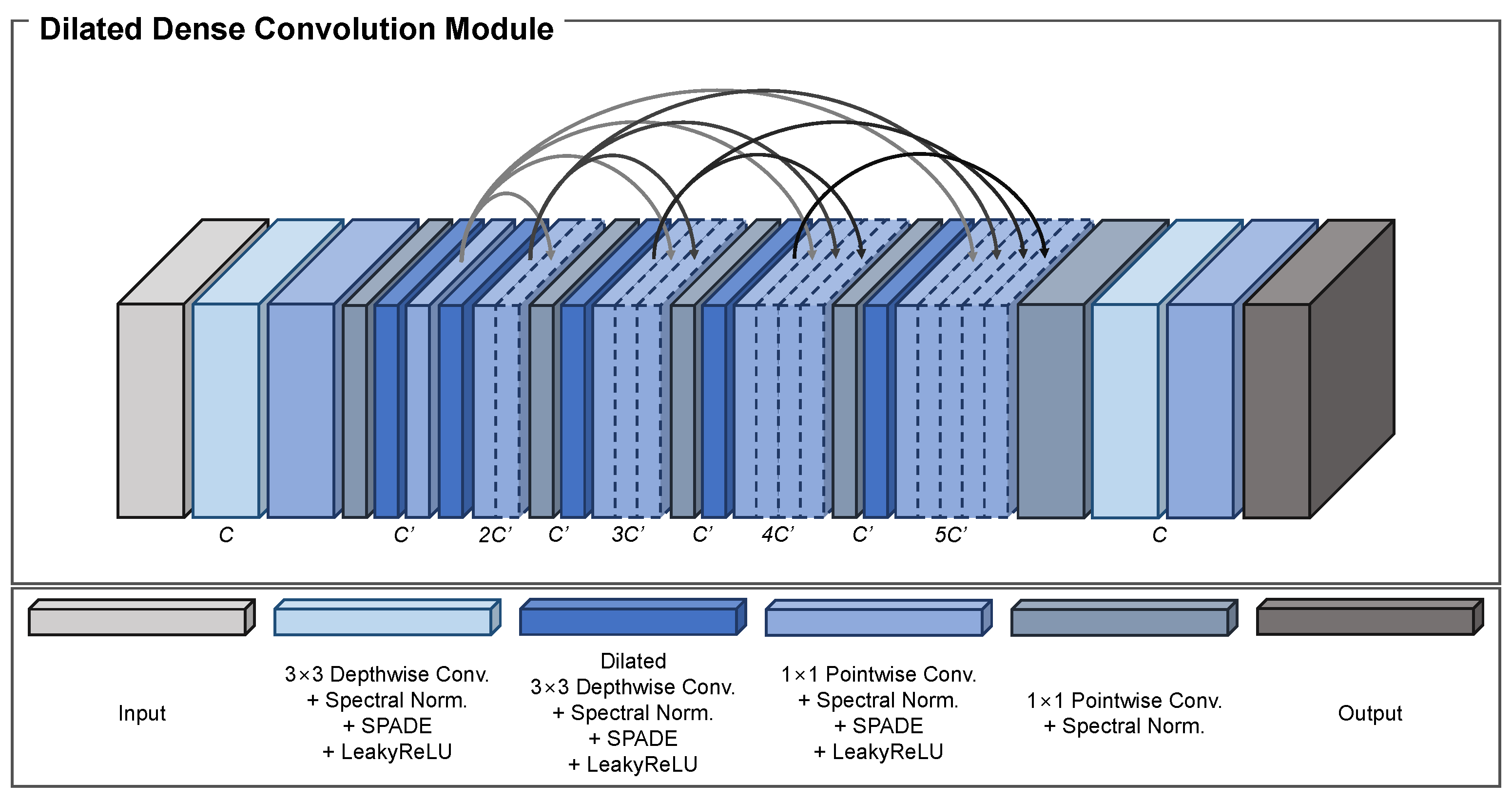
We propose the DDCM to fill-in the missing regions by combining various feature maps with different receptive fields in each stage. The main components of the DDCM are dense blocks [30] and dilated convolutional modules. We first explain the structure of the proposed DDCM and then present the reasons for suitability in image-inpainting tasks.
Given the input feature map F D D C M of size H × W × C that passes through depthwise and pointwise convolutional modules. To reduce the number of model parameters, a bottleneck layer with a pointwise convolutional layer reduces the number of channels to C to generate the feature map F D D C M 0 , which is expressed as
F D D C M 0 = B L P C D C ( F D D C M ) ,
where C = C 2 , and D C , P C , and B L denote the depthwise and pointwise convolutional module and bottleneck layer, respectively.
Then, a depthwise convolutional module with a dilation rate of two and a pointwise convolutional module were applied to obtain the feature map F D D C M 1 , which is formulated as
F D D C M 1 = P C D D C r = 2 ( F D D C M 0 ) ,
where D D C represents the dilated depthwise convolutional module with the subscript r denoting the dilation rate.
The same operation with a dilation rate of four was employed to extract the feature map F D D C M 2 , which is defined as
F D D C M 2 = P C D D C r = 4 ( F D D C M 1 ) .
Next, two feature maps, F D D C M 1 and F D D C M 2 , were concatenated channel-wise to produce [ F D D C M 1 , F D D C M 2 ] for feature aggregation. The combined feature map then went through the bottleneck layer to decrease the number of channels from 2 C to C . A depthwise convolutional module with a dilation rate of six and a pointwise convolutional module were applied to construct the feature map F D D C M 3 , which is expressed as
F D D C M 3 = P C D D C r = 6 B L ( [ F D D C M 1 , F D D C M 2 ] ) .
Using all the previous features, the same operation as in Equation 7 was applied to yield the feature maps F D D C M 4 and F D D C M 5 , which are formulated as
F D D C M 4 = P C D D C r = 8 B L ( [ F D D C M 1 , F D D C M 2 , F D D C M 3 ] )
F D D C M 5 = P C D D C r = 10 B L ( [ F D D C M 1 , F D D C M 2 , F D D C M 3 , F D D C M 4 ] ) .
Finally, all the extracted feature maps were combined into one feature map to utilize the effective information. This was then fed into the bottleneck layer to reduce the number of channels from 5 C to C. Depthwise and pointwise convolutional modules were applied to produce the final output F D D C M of size H × W × C , which is defined as
F D D C M = P C D C B L ( [ F D D C M 1 , F D D C M 2 , F D D C M 3 , F D D C M 4 , F D D C M 5 ] ) .
As the feature map was fed forward, the a dilation rate of the depthwise convolutional module increased by two. Increasing the dilation rate expanded the effective receptive field, which enabled the model to look over much larger areas of the feature map. This process is applicable to image-inpainting tasks because the network can fill-in the masked regions using various types of information from the entire feature map. A structural overview of the DDCM is shown in Figure 3.
The dense block was first introduced in [30] to mitigate the vanishing-gradient problem, enhance feature propagation, and stimulate the reuse of the feature map. For the DDCM, we employed the dense block for two main reasons.
The first reason is to help the model converge to a better minimum point. Because the DDCMs are located in the middle of the proposed method and skip the connections between the encoder and decoder, the gradient may vanish because of the deeply stacked convolutional modules. Hence, adding a dense block provides various paths to pass the gradient at the current location to the input, which eventually solves the gradient-vanishing problem.
The second reason is to gradually fill-in the missing areas in the feature map with the relevant pixels. Although the feature maps were extracted and downsampled to different scales, the missing areas were not provided with the appropriate values. Thus, the dense block was adopted to progressively generate pixels while inducing minimal artifacts. The feature maps at the front part of the DDCM (i.e., F D D C M 1 and F D D C M 2 ) were extracted using local information. Therefore, passing feature maps at every latter stage acted as the prior information, which helped the model continuously draw out features from local to global regions with an increased receptive field.
Thus, the DDCM is suitable for image-inpainting tasks for the aforementioned reasons. The effect of the DDCM is thoroughly analyzed in Section 4.7.

3.1.3. Efficient Self-Attention

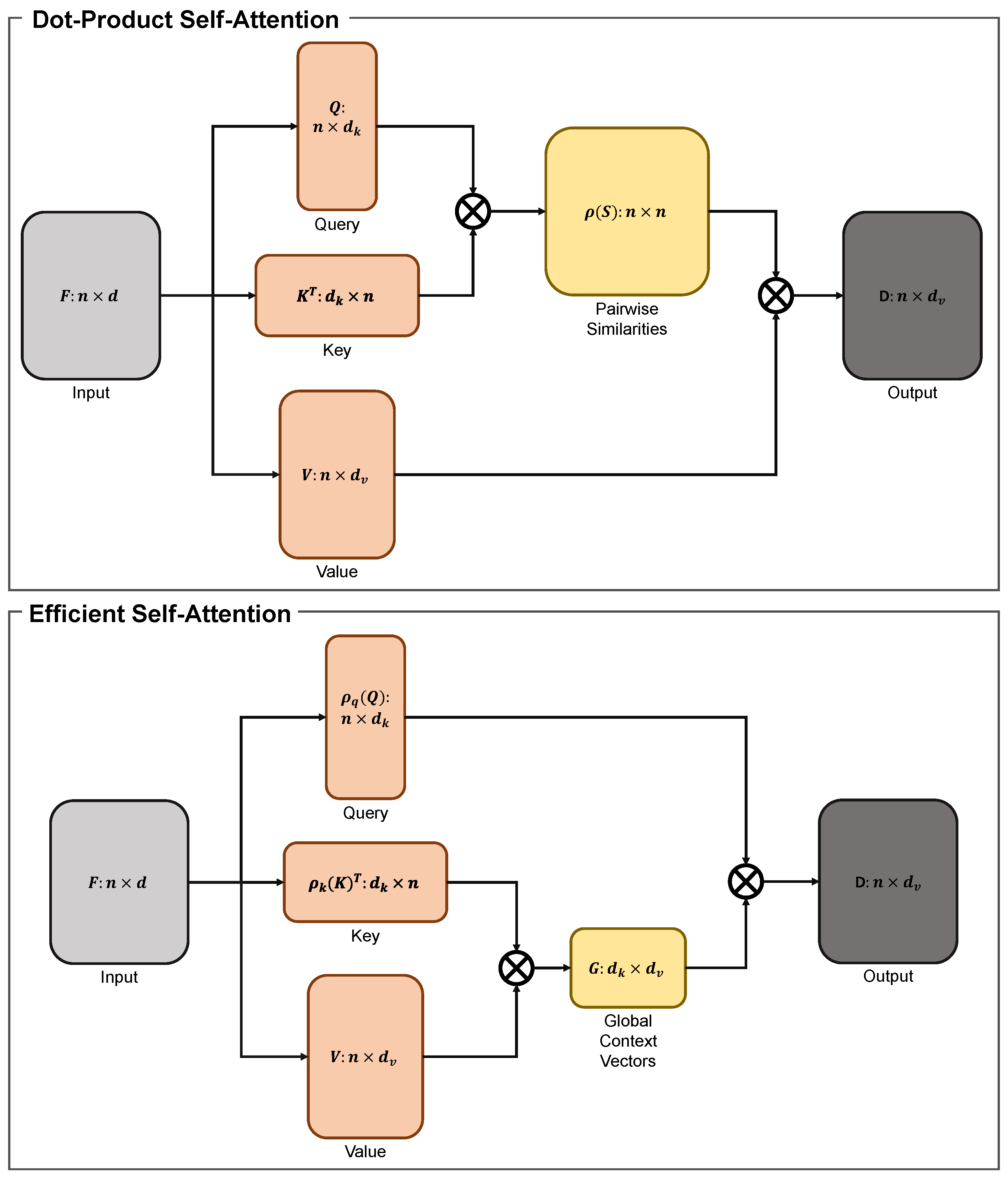
For our model, ESA [31] was employed to extract nonlocal information while retaining the minimum number of model parameters. In this section, we explain the details of ESA by comparing it with dot-product self-attention.
Dot-product self-attention [51] is a method to model long-range interactions in neural networks. Let f i R d be the input features of the i-th layer of a CNN. The dot-product self-attention utilizes three different linear layers to transform f i into three feature maps: query q i R d k , key k i R d k , and value v i R d v . For matrix multiplication, the queries and keys must have the same feature dimension d k . The similarity between the i-th query and j-th key was measured by ρ ( q i k j T ) , where ρ denotes a normalization function. Hence, the dot-product self-attention computes the similarities between all pairs of the position in the feature maps. By utilizing the relationships as weights, the output feature was obtained by the weighted summation of the values from all positions that were aggregated at the position i.
Assuming that all n positions’ queries, keys, and values in the matrix formed as Q R n × d k , K R n × d k , and V R n × d v , the output of the dot-product self-attention is defined as
D ( Q , K , V ) = ρ ( Q K T ) V ,
where ⊗ represents the matrix multiplication. There are two main choices for the normalization function ρ .
S c a l i n g : ρ ( Z ) = Z n S o f t m a x : ρ ( Z ) = δ r o w ( Z ) ,
where δ r o w is the adopted Softmax function in each row of matrix Z .
The main obstacle to using this mechanism is the resource demands. This operation calculated the relationship between each pair of positions, which induced n 2 similarities. Hence, it yielded a memory and computational complexity of O ( n 2 ) and O ( d k n 2 ) , respectively, where O denotes the large O notation. Owing to the resource demands, this mechanism is mainly applied to low-resolution features.
Shen et al. [31] proposed an efficient self-attention mechanism that is mathematically identical to the dot-product self-attention but significantly faster and more memory-efficient. This mechanism also applies three linear layers to the input feature F R n × d to form the queries Q R n × d k , keys K R n × d k , and values V R n × d v . Unlike the dot-product self-attention mechanism, which solves the keys as n feature vectors in R d k , the efficient module considers them as d k single-channel feature maps. This module then generates a global context vector by utilizing each of these feature maps as weights over all areas, and accumulating the value features through weighted summation.
Thus, the efficient self-attention mechanism is expressed as
E ( Q , K , V ) = ρ q ( Q ) ( ρ k ( K ) T V ) ,
where ρ q and ρ k denote the normalization functions for the query and key features, respectively. The two normalization approaches are formulated as
S c a l i n g : ρ q ( Z ) = ρ k ( Z ) = Z n S o f t m a x : ρ q = δ r o w ( Z ) , ρ k = δ c o l ( Z ) ,
where δ q and δ k are the Softmax functions for each row or column of the matrix Z , respectively.
The efficient self-attention is equal to the dot-product self-attention when the scaling normalization method is employed. Substituting the scaling normalization formula in Equation 12 into Equation 11 yields
D ( Q , K , V ) = Q K T n V .
Similarly, substituting the scaling normalization formula in Equation 14 into Equation 13 produces
E ( Q , K , V ) = Q n ( K T n V ) .
Because n is scalar and matrix multiplication is associative, Equation 16 is formulated as
E ( Q , K , V ) = Q n ( K T n V ) = 1 n Q ( K T V ) = 1 n ( Q K T ) V = Q K T n V .
As result, correlating Equation 15 and 17 yields E ( Q , K , V ) = D ( Q , K , V ) . A structural overview of the dot product and its efficient self-attention is shown in Figure 4.
Owing to the effective implementation and efficiency of the attention mechanism, we employed ESA at the decoder to extract long-range information on aggregated features and obtain clues from other areas to successfully fill-in the missing areas. The impact of ESA is examined in detail in Section 4.7.

3.2. Discriminator Architecture

For adversarial learning, we adopted a multiscale discriminator framework. The discriminator has a PatchGAN [52] structure with five 4 × 4 vanilla convolution layers and step size of { 2 , 2 , 2 , 1 , 1 } . For the first three convolutional layers, the spatial size of each output feature map was halved, while the number of channels was doubled. The fourth convolutional layer also doubled the number of channels, while the last convolutional layer transformed the final output feature map into a map with one channel. For all convolutional layers, spectral normalization [50] was adopted to satisfy the 1-Lipschitz constraint and ensure the training process. The LReLU was used as the activation function with a hyperparameter of 0.2.
To apply a conditional setting for the learning process, the generated and target images were concatenated channel-wise with the corresponding binary mask M , and fed into the discriminator as the input. In addition, both inputs were downsampled by half using nearest-neighbor interpolation and fed into another discriminator to satisfy the multiscale discriminator framework. The output sizes of the two discriminators are 30 × 30 × 1 and 14 × 14 × 1 . A structural overview of the multiscale discriminator framework is shown in Figure 1.

3.3. Loss Function

To train our model, we used a combination of loss functions, namely, the adversarial loss [19], feature-matching (FM) loss [53], perceptual loss [54], style loss [55], and reconstruction loss.
First, for the adversarial loss, we employed the hinge loss [56] as the objective function for the generator, which is defined as
L a d v G 1 = E [ M , I o u t ] [ D 1 ( [ M , I o u t ] ) ] L a d v G 2 = E [ M , I o u t ] [ D 2 ( [ M , I o u t ] ) ] ,
where I o u t denotes the output image from the generator, ↓ is the nearest-neighbor interpolation downsampled by half, and D 1 and D 2 are discriminators with inputs of different scales. The objective functions of the two discriminators are expressed as
L a d v D 1 = E [ M , I t a r g e t ] [ R e L U ( 1 D 1 ( [ M , I t a r g e t ] ) ) ] + E [ M , I o u t ] [ R e L U ( 1 + D 1 ( [ M , I o u t ] ) ) ] L a d v D 2 = E [ M , I t a r g e t ] [ R e L U ( 1 D 2 ( [ M , I t a r g e t ] ) ) ] + E [ M , I o u t ] [ R e L U ( 1 + D 2 ( [ M , I o u t ] ) ) ] ,
where I t a r g e t is the target image and R e L U is the rectified linear unit (ReLU) activation function.
Second, we utilized the FM loss. The FM loss caused the generator to create more reasonable and realistic outputs by measuring the features of the output image I o u t and target image I t a r g e t in each of the discriminators. Let S 1 and S 2 be the number of convolutional layers of D 1 and D 2 ; E k 1 and E k 2 the number of elements in the kth activation layer of D 1 and D 2 ; and D k 1 and D k 2 the activation diagram of layer k of D 1 and D 2 , respectively. The FM loss is defined as
L f m 1 = E k = 1 S 1 1 E k 1 D k 1 ( I t a r g e t ) D k 1 ( I o u t ) 1 1 L f m 2 = E k = 1 S 2 1 E k 2 D k 2 ( I t a r g e t ) D k 2 ( I o u t ) 1 1 ,
The mean absolute error (MAE) was adopted to compute the distance between features.
Third, we used the perceptual loss, which compares the feature maps acquired using the same convolution operation for the target and output images. This loss enables the generator to enhance the high-level semantic correlation between the two images by calculating and minimizing their differences. Specifically, we compared the distances between the activation features of the five layers (relu1-1, relu2-1, relu3-1, relu4-1, and relu5-1) of the target and generated images in the VGG-19 network [57] trained on the ImageNet dataset [58]. Thus, the perceptual loss is formulated as
L p e r c = E k 1 E k τ k ( I t a r g e t ) τ k ( I o u t ) 1 1 ,
where E k denotes the number of elements in the kth activation layer and τ k denotes the activation diagram of the correlated layer.
Fourth, we applied the style loss, which is the correlation coefficient activation value of each activation feature channel. In our method, the VGG-19 network was used to extract feature maps as in L p e r c . Its correlation is defined by computing the eccentric covariance between the diverse activation characteristic graphs of various scales. The style loss is expressed as
L s t y l e = E k G k τ ( I t a r g e t ) G k τ ( I o u t ) 1 1 ,
where k denotes the kth activation layer and G k τ is the Gram matrix τ k with a size of C k × C k .
Finally, we adopted the reconstruction loss to compute the distance between the corresponding pixels of the target and output images. As in the FM, perceptual, and style losses, the MAE was used to calculate the difference because it mitigated the problem of exploding gradients by maintaining a stable gradient for any input. The reconstruction loss is defined as
L r e c = I t a r g e t ( 1 M ) I o u t ( 1 M ) 1 1 ,
where only the restored areas were used to compute the loss.
Using all of the abovementioned losses, the overall loss function of our model is formulated as
L P E I P N e t = λ a d v ( L a d v G 1 + L a d v G 2 ) + λ f m ( L f m 1 + L f m 2 ) + λ p e r c L p e r c + λ s t y l e L s t y l e + λ r e c L r e c ,
where the loss weights are set as follows: λ a d v = 1 , λ f m = 1 × 10 2 , λ p e r c = 1 × 10 2 , λ s t y l e = 1 × 10 2 , and λ r e c = 1 × 10 3 .

4. Experiments

4.1. Datasets

The PEIPNet was trained on three public datasets: Paris StreetView [59], CelebA [60], and Places2 [61]. The Paris StreetView dataset contains 15,900 training samples and 100 testing images. The CelebA human face dataset contains approximately 160,000 training images and 19,900 testing images. The standard training dataset Places2 contains over four million images. Our model was evaluated on this validation dataset with 36,500 images. For training and testing, we followed the same procedure as in [14], in which random augmentation methods, such as random translation, rotation, dilation, and cropping, were used to augment the training masks, A mask set with 12,000 irregular masks that were pre-organized into six intervals according to the mask area ( 1 % 10 % , 10 % 20 % , , 50 % 60 % ) was employed for testing. All the images in the Paris StreetView, CelebA, and Place2 datasets were resized to 256 × 256 using bicubic interpolation.

4.2. Compared Methods

We compared our method with state-of-the-art models, such as EC [24], RFR [62], CR-Fill [63], CTSDG [64], and SPL [65]. All these models were pretrained; hence, their performance was directly evaluated in our settings.

4.3. Implementation Details

In the experiments, we used the Adam optimizer [66] ( β 1 = 0.9 , β 2 = 0.999 ). The learning rates were initialized to 1 × 10 3 and 4 × 10 3 for the generator and discriminators, respectively. The batch size was set to 32. Our model was trained for 1 × 10 5 iterations, with the model evaluated at each 1 × 10 3 iteration. The cosine annealing algorithm [67] was selected as the learning rate scheduler to slowly decay the learning rates of the generator and discriminators to 1 × 10 5 and 4 × 10 5 , respectively. The PyTorch framework [68] and an NVIDIA A100 GPU with 80 GB of RAM were utilized to implement the proposed method. (The official code will be uploaded on GitHub when this paper is accepted.)

4.4. Analysis of Model Complexity

Because we introduced a lightweight architecture for the image-inpainting task, the number of parameters and operational memory of each model was computed and compared, as listed in Table 1. Models with a batch size of one were used to measure the memory usage. For the model capacity, our method had less than one million parameters, which is the smallest among the models. The parameter difference ratio compared with other approaches ranged from 4.5 to 57.9. For the operational memory, PEPSI [21] would be an exceptional comparison, but was excluded because the official code was not provided by its authors. Our model also consumed the least amount of computational resources, i.e., approximately seven times lower compared with CR-Fill, the model with the second-lowest consumption. Having the most efficient structure in terms of both the number of parameters and operational memory provides a significant advantage in solving the overfitting problem, which commonly occurs when using a dataset with a limited number of images.

4.5. Qualitative Evaluations

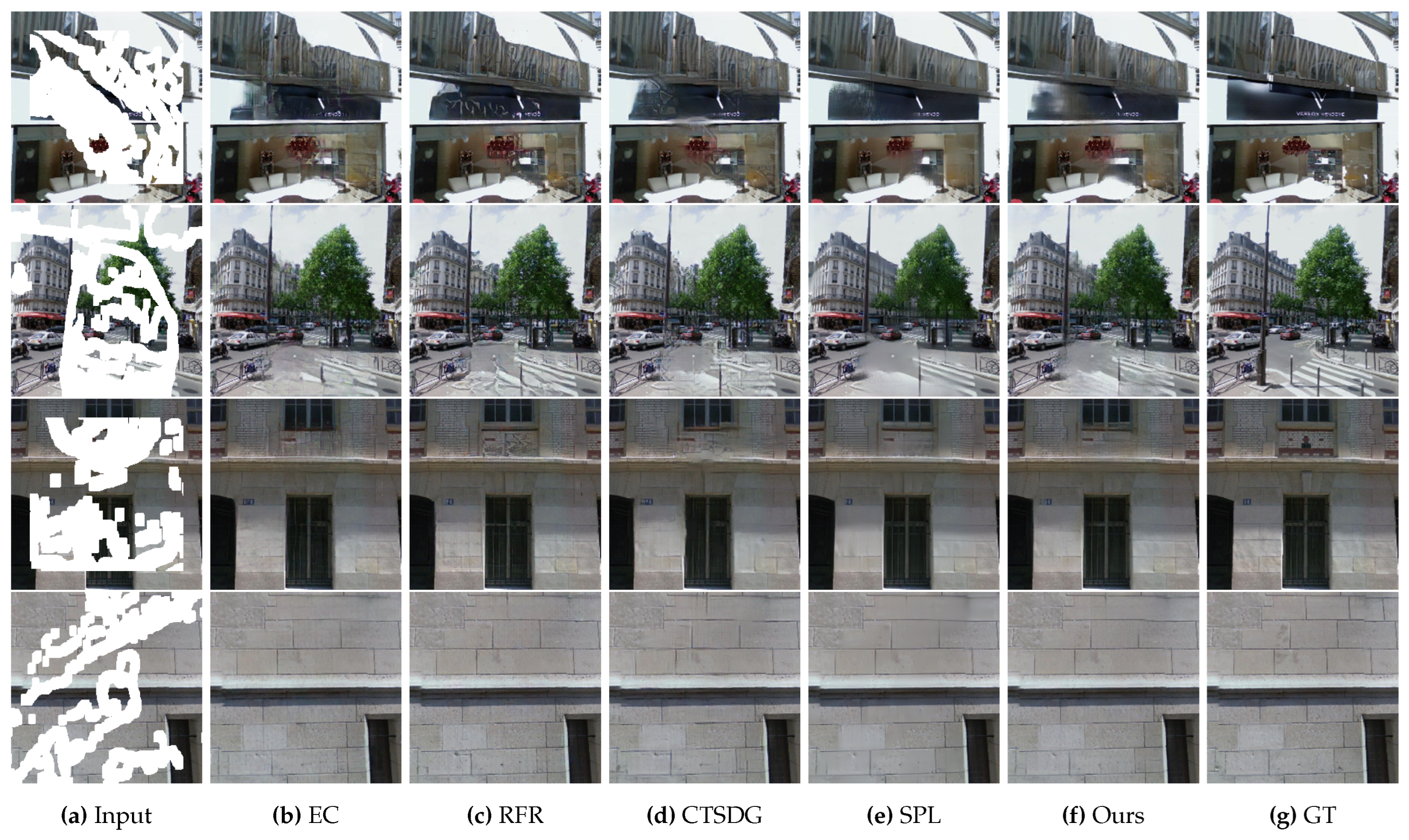
Figure 5 shows the qualitative comparison results on the Paris StreetView dataset. The EC generated an edge map corresponding to the final output and identified the global arrangement and long-range features by employing dilated convolutional layers. However, minute textural details were not extracted, resulting in an offset in the local target. For example, in the first row, the straight line above the front sign was not recovered, which corrupted the distinct boundary. In the second to fourth rows, the texture of the tree, the structure of the bricks between the middle highest window, and the pattern of the building surface were distorted. RFR sequentially filled-in the missing pixels by circular feature inference, which generated high-fidelity visual effects; however, serious artifacts developed. For example, in the first to third rows, wrinkled patterns were produced in the large masked regions. In the fourth row, checkerboard artifacts were found on the bricks, which is a common problem of transposed convolutional layers [69]. CTSDG bound the texture and structure to each other; however, the boundaries were blurred owing to the implicit usage of the structure. For instance, in the first to third rows, the straight lines were obscured, which distorted the distinct boundaries of semantically different regions. In the fourth row, cross-patterned deformities developed throughout the region. SPL conducted knowledge distillation on the pretext models and modified the features for image-inpainting. These not only helped in understanding the global context but also provided structural supervision for the restoration of the local texture. Nonetheless, the local texture was still smoothed out, which resulted in blurring effects. For example, although solid lines were retained in all the rows, the texture of the leaves and brick patterns were not retained in the second to fourth rows, respectively. In contrast, our proposed method restored images with a suitable balance of low- and high-level features. For all rows, the pixels were filled with clear boundaries and a semantically plausible texture, as seen in the second row. This result is attributed to the use of ESA, where the model obtained hints on the texture from all areas of the corresponding feature maps.
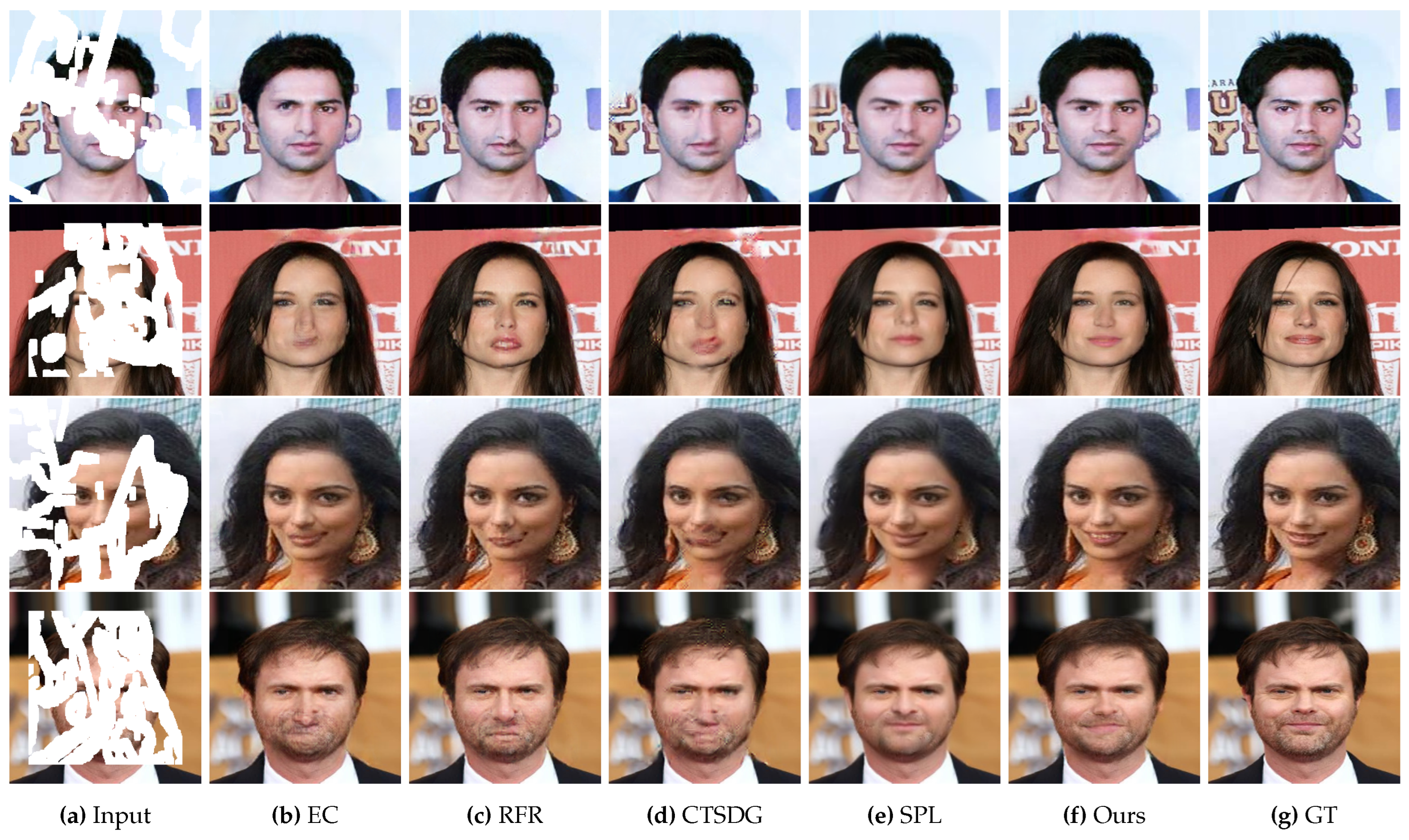
Figure 6 shows the qualitative comparison results on the CelebA dataset. EC obtained unsatisfactory results, i.e., the facial structures were extremely distorted. For instance, in the first row, the position of the left eye was not symmetrical to the right eye. In the second row, the nose did not have the appropriate shape, while the mouth was barely visible. In the fourth row, although the eyes and nose had the proper silhouettes, the mouth was hardly seen. RFR provided better results than EC, but the final outputs did not improve. Although the model generated eyes with a normal shape, the mouths in all the rows were distorted, which ruined the degree of image restoration. CTSDG had the least favorable results. For all rows, the facial structures were not retained due to blurring effects, and checkerboard artifacts were found in all inpainted regions. SPL sufficiently recovered the images, but there were still some implausible regions remained. For instance, in the first row, the size of the left eye was different and relatively smaller than the right eye. In the fourth row, the wrinkles and beard on the face disappeared owing to excessive smoothing. In contrast, our model generated images with the best quality. For example, in the first row, the size of the left eye was similar to that of the right eye, and was at a suitable location. In the third row, unlike the other models, our method generated a mouth with teeth that was very close to the ground-truth image. In the fourth row, the wrinkles and beard with a proper mouth were retained, which has the least perceived difference compared with the other methods.
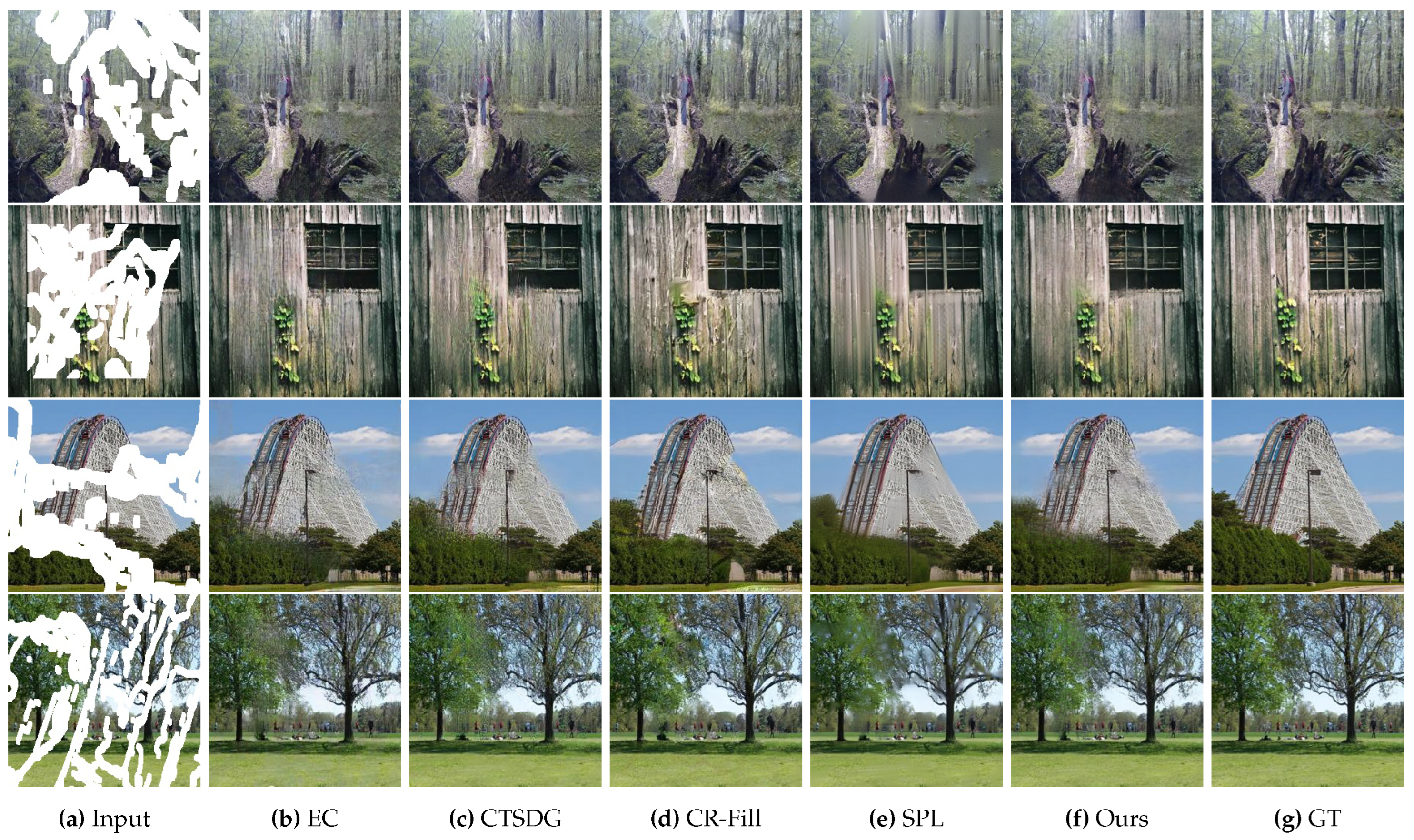
Figure 7 shows the qualitative comparison results on the Places2 dataset. EC restored images with an acceptable quality using an edge map; however, some areas were not appealing. For example, in the third row, the rails of the roller coaster were connected by curved lines, which is unrealistic. In the fourth row, the leaves filled with generated pixels did not have a consistent color compared with the other regions. CTSDG produced images with indistinct boundaries, i.e., unrealistic results. For instance, in the second row, the structure of the window was not fully retained owing to the blurriness of the bottom-left region. In the third row, the ride paths appeared disconnected, which is unrealistic. In the fourth row, the texture of the leaves contrasted with the other regions and was not harmonized with different areas. CR-Fill trained the generator by adopting an auxiliary contextual reconstruction task that made the generated output more plausible, even when restored by the surrounding regions. Hence, CR-Fill reconstructed images with an acceptable quality; however, some regions were still perceived as different. For instance, in the first and third rows, the boundaries of the trees were not obvious, and the color of the middle-right part of the ride was inconsistent. SPL produced outputs with distinct lines connecting the masked regions; however, key textures and patterns were lost owing to excessive smoothing. For example, in the first, third, and fourth rows, the textures of the objects were blurred. The generated image in the second row contained checkerboard artifacts that distorted the texture and quality of the image. In contrast to other methods, our proposed model achieved a balance between the apparent boundaries and textures of various objects. For instance, all the rows had straight lines that separated semantically different areas. Furthermore, the textures of the objects were effectively restored, leading to plausible results.
In summary, our proposed method effectively balanced low- and high-level feature restoration. This proves the generalizability of the proposed method based on qualitative evaluations.

4.6. Quantitative Evaluations

To analyze the inpainting results of our proposed method and those of other models, we applied four different metrics: Fréchet inception distance (FID) [70], learned perceptual image patch similarity (LPIPS) [71], structural similarity (SSIM), and peak signal-to-noise ratio (PSNR). The FID is a widely used quantitative metric in the field of image generation that measures the Wasserstein-2 distance between the generated and target images utilizing a pretrained Inception-V3 model [46]. Except for the FID, the other metrics are full-reference image quality assessments, in which restored images are compared with their corresponding ground-truth images. The LPIPS evaluates the restoration effect by computing the similarity between the deep features of two images using AlexNet [72]. The SSIM calculates the difference between two images in terms of their brightness, contrast, and structure. Finally, the PSNR analyzes the restoration performance by measuring the distances between the pixels of two images. The quantitative comparison results on the Paris StreetView, CelebA, and Places2 datasets are listed in Table 2, Table 3, and Table 4, respectively. For all the results, the first and second highest values are labeled in bold and underlined (↓ lower is better; ↑ higher is better).
On the Paris StreetView dataset, our PEIPNet method was ranked as the first or second for all metrics. For mask rates of ( 0.1 , 0.2 ] and ( 0.2 , 0.3 ] , PEIPNet achieved the best results, similar to the FID and LPIPS. However, for mask rates of ( 0.3 , 0.4 ] and ( 0.4 , 0.5 ] , RFR had the best results, similar to the FID and LPIPS, while PEIPNet had the second-best results. For SSIM and PSNR, SPL and PEIPNet had the best and second-best results, respectively, for all mask rates. The excellent performance of PEIPNet was attributed to the few artifacts in the generated images. The textures of different objects were also retained, which FID and LPIPS are highly sensitive to. Hence, PEIPNet can fill-in small masked regions, but its strength decreased in the large-hole inpainting task. This is because DDCM and ESA encouraged PEIPNet to obtain various meaningful hints from different regions of the feature maps with small masked areas by identifying global long-range and local features with dilated convolution and nonlocal attention. If there are insufficient regions from which to obtain information, the aforementioned mechanism reduced the performance of PEIPNet.
On the CelebA dataset, PEIPNet was ranked as the first or second best for the LPIPS, SSIM, and PSNR. EC had the best outcomes for the FID with all mask rates, followed by SPL. However, the FID difference between SPL and PEIPNet was very small, except with the mask rate of ( 0.4 , 0.5 ] . For the LPIPS, PEIPNet had the best results with the first three mask rates and the second-best with the highest mask rate. The opposite is true for the first and second-best results of the RFR. For the SSIM and PSNR, SPL had the best values, followed by PEIPNet. As on the Paris StreetView dataset, the disparity in inpainting performance compared with the best method continued to increase as the mask rate increased owing to the aforementioned reason.
On the Places2 dataset, PEIPNet again had either the best or second-best LPIPS, SSIM, and PSNR. Unlike on the CelebA dataset, PEIPNet also had the second-best outcome for the FID with mask rates of ( 0.1 , 0.2 ] and ( 0.2 , 0.3 ] . For the LPIPS, PEIPNet had the lowest values with the first three mask rates, and the second lowest with the highest mask rate; the opposite is true for SPL. For the SSIM and PSNR, PEIPNet had the second highest values for all mask rates, while SPL had the best outcomes. The same phenomenon of the increased inpainting accuracy difference compared with the best result was also observed on the Places2 dataset.
The proposed PEIPNet method showed exceptional performance for all metrics: FID, LPIPS, SSIM, and PSNR. In most cases, PEIPNet had the best or second-best outcome; this tendency was not observed in the other methods. Specifically, PEIPNet achieved at least the second-best results on the Paris StreetView dataset, indicating the advantage of having a small number of model parameters when training with a limited number of samples. Thus, the quantitative evaluations confirmed the generalizability of the proposed method.

4.7. Ablation Studies

To verify the effects of the introduced the DDCM and ESA, ablation studies using our method were conducted on the Paris StreetView dataset. Specifically, we divided the DDCM into two parts for analysis: dilated convolution and dense block. To reduce the training time, we altered the batch size to eight for all combinations.
The quantitative results with different combinations of DDCM and ESA on the Paris StreetView dataset are listed in Table 5. For the DDCM, eliminating the entire module affected the model performance, where the average FID and LPIPS increased by 5.3607 and 0.0102, while the SSIM and PSNR decreased by 0.0083 and 0.4658, respectively, compared with the original model. Comparison of the two parts of the DDCM showed that applying dilated convolutional layers yielded better results for all metrics, which indicates the importance of long-range feature extraction in the image-inpainting task. ESA plays a crucial role because the average FID and LPIPS increased by 2.32 and 0.0034, while the SSIM and PSNR decreased by 0.0025 and 0.0676, respectively. However, the decline in the ESA performance was lower than that of the DDCM, indicating its dominance in the proposed method.
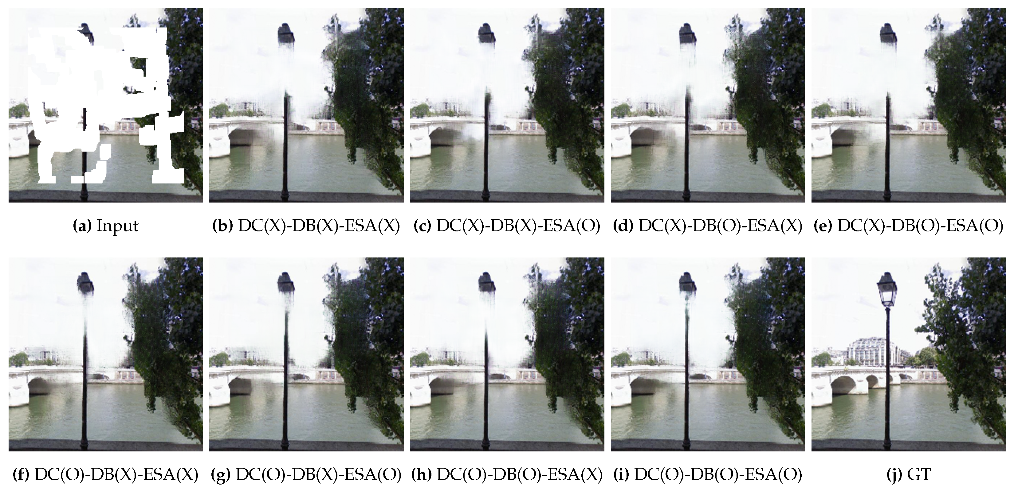
The qualitative results with different combinations of the DDCM and ESA on the Paris StreetView dataset are shown in Figure 8. Unlike the original model, the remaining combinations did not retain the streetlight structure. Specifically, the pillar was disconnected from the head of the lamp, which is unrealistic. The authentic model provided the best restoration of the texture of the leaves, demonstrating the strength of the proposed modules.
Finally, we calculated the complexities of different combinations of models, as described in Section 4.4 and summarized in Table 6. The contribution of dilated convolution was minor because there was almost no change in the memory when this process was eliminated. Removing the dense block had a greater impact on the memory compared with dilated convolution, but the change remained insignificant. On the other hand, eliminating ESA had a significant impact on the memory through a 4.51% reduction in the computational cost. Thus, adopting self-attention remains costly despite its structural efficiency.

5. Conclusion

In this study, we introduced the PEIPNet model to fill-in the missing pixels in damaged images. The proposed method has a one-stage inpainting framework, in which depthwise and pointwise convolutions were utilized to minimize the number of parameters and computational costs. We introduced three distinct modules into our model to produce semantically plausible outputs. First, SPADE was adopted to normalize the feature maps according to the input mask. Second, DDCM was used at each scale to generate pixels and capture global information along the activations. Finally, we employed ESA to extract long-range information and obtain references from undamaged areas. Our model consumed the lowest amount of operational memory compared with state-of-the-art models, demonstrating its potential. In addition, the experiments showed that the proposed method can be generalized in terms of both qualitative and quantitative perspectives. In future studies, we plan to refine PEIPNet to obtain higher-resolution images for real-world applications.

Author Contributions

Conceptualization, J.K. and W.C.; methodology, J.K. and W.C.; software, J.K. and W.C.; validation, J.K. and W.C.; formal analysis, J.K. and W.C.; investigation, J.K. and W.C.; resources, J.K. and W.C.; data curation, J.K. and W.C.; writing—original draft preparation, J.K. and W.C.; writing—review and editing, J.K., W.C. and S.L.; visualization, J.K. and W.C.; supervision, S.L.; project administration, S.L. All authors have read and agreed to the published version of the manuscript.

Funding

This research received no external funding.

Institutional Review Board Statement

Not applicable.

Informed Consent Statement

Not applicable.

Data Availability Statement

The data presented in this study are openly available.

Conflicts of Interest

The authors declare no conflict of interest.

References

  1. Efros, A.A.; Leung, T.K. Texture synthesis by non-parametric sampling. seventh IEEE international conference on computer vision (ICCV). IEEE, 1999, Vol. 2, pp. 1033–1038.
  2. Ballester, C.; Bertalmio, M.; Caselles, V.; Sapiro, G.; Verdera, J. Filling-in by joint interpolation of vector fields and gray levels. IEEE Transactions on Image Processing 2001, 10, 1200–1211. [Google Scholar] [CrossRef]
  3. Efros, A.A.; Freeman, W.T. Image Quilting for Texture Synthesis and Transfer. 28th Annual Conference on Computer Graphics and Interactive Techniques, 2001, p. 341–346.
  4. Bertalmio, M.; Vese, L.; Sapiro, G.; Osher, S. Simultaneous structure and texture image inpainting. IEEE transactions on image processing 2003, 12, 882–889. [Google Scholar] [CrossRef] [PubMed]
  5. Criminisi, A.; Perez, P.; Toyama, K. Region filling and object removal by exemplar-based image inpainting. IEEE Transactions on Image Processing 2004, 13, 1200–1212. [Google Scholar] [CrossRef] [PubMed]
  6. Tang, F.; Ying, Y.; Wang, J.; Peng, Q. A Novel Texture Synthesis Based Algorithm for Object Removal in Photographs. Advances in Computer Science - ASIAN 2004. Higher-Level Decision Making, 2005, pp. 248–258.
  7. Cheng, W.H.; Hsieh, C.W.; Lin, S.K.; Wang, C.W.; Wu, J.L. Robust algorithm for exemplar-based image inpainting. International Conference on Computer Graphics, Imaging and Visualization, 2005, pp. 64–69.
  8. Simakov, D.; Caspi, Y.; Shechtman, E.; Irani, M. Summarizing visual data using bidirectional similarity. 2008 IEEE conference on computer vision and pattern recognition. IEEE, 2008, pp. 1–8.
  9. Barnes, C.; Shechtman, E.; Finkelstein, A.; Goldman, D.B. PatchMatch: A randomized correspondence algorithm for structural image editing. ACM Trans. Graph. 2009, 28, 24. [Google Scholar] [CrossRef]
  10. Pathak, D.; Krahenbuhl, P.; Donahue, J.; Darrell, T.; Efros, A.A. Context encoders: Feature learning by inpainting. IEEE conference on computer vision and pattern recognition (CVPR), 2016, pp. 2536–2544.
  11. Yu, F.; Koltun, V. Multi-Scale Context Aggregation by Dilated Convolutions. 4th International Conference on Learning Representations (ICLR), 2016.
  12. Iizuka, S.; Simo-Serra, E.; Ishikawa, H. Globally and locally consistent image completion. ACM Transactions on Graphics (ToG) 2017, 36, 1–14. [Google Scholar] [CrossRef]
  13. Ding, D.; Ram, S.; Rodríguez, J.J. Image inpainting using nonlocal texture matching and nonlinear filtering. IEEE Transactions on Image Processing 2018, 28, 1705–1719. [Google Scholar] [CrossRef] [PubMed]
  14. Liu, G.; Reda, F.A.; Shih, K.J.; Wang, T.C.; Tao, A.; Catanzaro, B. Image Inpainting for Irregular Holes Using Partial Convolutions. European Conference on Computer Vision (ECCV), 2018, pp. 89–105.
  15. Wang, Y.; Tao, X.; Qi, X.; Shen, X.; Jia, J. Image inpainting via generative multi-column convolutional neural networks. Advances in neural information processing systems 2018, 31. [Google Scholar]
  16. Yan, Z.; Li, X.; Li, M.; Zuo, W.; Shan, S. Shift-net: Image inpainting via deep feature rearrangement. European conference on computer vision (ECCV), 2018, pp. 1–17.
  17. Yu, J.; Lin, Z.; Yang, J.; Shen, X.; Lu, X.; Huang, T.S. Generative image inpainting with contextual attention. IEEE conference on computer vision and pattern recognition (CVPR), 2018, pp. 5505–5514.
  18. Li, J.; He, F.; Zhang, L.; Du, B.; Tao, D. Progressive reconstruction of visual structure for image inpainting. IEEE/CVF international conference on computer vision (ICCV), 2019, pp. 5962–5971.
  19. Goodfellow, I.; Pouget-Abadie, J.; Mirza, M.; Xu, B.; Warde-Farley, D.; Ozair, S.; Courville, A.; Bengio, Y. Generative Adversarial Nets. Advances in Neural Information Processing Systems (NIPS), 2014, Vol. 27.
  20. Liu, H.; Jiang, B.; Xiao, Y.; Yang, C. Coherent semantic attention for image inpainting. IEEE/CVF International Conference on Computer Vision (ICCV), 2019, pp. 4170–4179.
  21. Sagong, M.c.; Shin, Y.g.; Kim, S.w.; Park, S.; Ko, S.j. Pepsi: Fast image inpainting with parallel decoding network. IEEE/CVF conference on computer vision and pattern recognition (CVPR), 2019, pp. 11360–11368.
  22. Zeng, Y.; Fu, J.; Chao, H.; Guo, B. Learning pyramid-context encoder network for high-quality image inpainting. IEEE/CVF conference on computer vision and pattern recognition (CVPR), 2019, pp. 1486–1494.
  23. Yu, J.; Lin, Z.; Yang, J.; Shen, X.; Lu, X.; Huang, T.S. Free-form image inpainting with gated convolution. IEEE/CVF international conference on computer vision (ICCV), 2019, pp. 4471–4480.
  24. Nazeri, K.; Ng, E.; Joseph, T.; Qureshi, F.; Ebrahimi, M. EdgeConnect: Structure Guided Image Inpainting using Edge Prediction. The IEEE International Conference on Computer Vision (ICCV) Workshops, 2019.
  25. Ren, Y.; Yu, X.; Zhang, R.; Li, T.H.; Liu, S.; Li, G. Structureflow: Image inpainting via structure-aware appearance flow. IEEE/CVF international conference on computer vision, 2019, pp. 181–190.
  26. Xiong, W.; Yu, J.; Lin, Z.; Yang, J.; Lu, X.; Barnes, C.; Luo, J. Foreground-aware image inpainting. IEEE/CVF conference on computer vision and pattern recognition (CVPR), 2019, pp. 5840–5848.
  27. Yang, J.; Qi, Z.; Shi, Y. Learning to incorporate structure knowledge for image inpainting. AAAI conference on artificial intelligence (AAAI), 2020, pp. 12605–12612.
  28. Howard, A.G.; Zhu, M.; Chen, B.; Kalenichenko, D.; Wang, W.; Weyand, T.; Andreetto, M.; Adam, H. MobileNets: Efficient Convolutional Neural Networks for Mobile Vision Applications. 2017, arXiv:cs.CV/1704.04861. [Google Scholar]
  29. Park, T.; Liu, M.Y.; Wang, T.C.; Zhu, J.Y. Semantic Image Synthesis With Spatially-Adaptive Normalization. IEEE/CVF Conference on Computer Vision and Pattern Recognition (CVPR), 2019.
  30. Huang, G.; Liu, Z.; van der Maaten, L.; Weinberger, K.Q. Densely Connected Convolutional Networks. IEEE Conference on Computer Vision and Pattern Recognition (CVPR), 2017.
  31. Shen, Z.; Zhang, M.; Zhao, H.; Yi, S.; Li, H. Efficient Attention: Attention With Linear Complexities. IEEE/CVF Winter Conference on Applications of Computer Vision (WACV), 2021, pp. 3531–3539.
  32. Telea, A. An image inpainting technique based on the fast marching method. Journal of graphics tools 2004, 9, 23–34. [Google Scholar] [CrossRef]
  33. Lowe, D.G. Object recognition from local scale-invariant features. seventh IEEE international conference on computer vision (ICCV), 1999, Vol. 2, pp. 1150–1157.
  34. Ioffe, S.; Szegedy, C. Batch Normalization: Accelerating Deep Network Training by Reducing Internal Covariate Shift. 32nd International Conference on Machine Learning (ICML), 2015, Vol. 37, pp. 448–456.
  35. Ulyanov, D.; Vedaldi, A.; Lempitsky, V. Instance Normalization: The Missing Ingredient for Fast Stylization. 2016, arXiv:cs.CV/1607.08022. [Google Scholar]
  36. Ba, J.L.; Kiros, J.R.; Hinton, G.E. Layer Normalization. 2016, arXiv:stat.ML/1607.06450. [Google Scholar]
  37. Wu, Y.; He, K. Group normalization. European conference on computer vision (ECCV), 2018, pp. 3–19.
  38. Dumoulin, V.; Shlens, J.; Kudlur, M. A Learned Representation For Artistic Style. 2017, arXiv:cs.CV/1610.07629. [Google Scholar]
  39. Huang, X.; Belongie, S. Arbitrary style transfer in real-time with adaptive instance normalization. IEEE international conference on computer vision (ICCV), 2017, pp. 1501–1510.
  40. De Vries, H.; Strub, F.; Mary, J.; Larochelle, H.; Pietquin, O.; Courville, A.C. Modulating early visual processing by language. Advances in Neural Information Processing Systems (NIPS), 2017, Vol. 30.
  41. Yu, T.; Guo, Z.; Jin, X.; Wu, S.; Chen, Z.; Li, W.; Zhang, Z.; Liu, S. Region normalization for image inpainting. AAAI conference on artificial intelligence, 2020, pp. 12733–12740.
  42. Sifre, L. Rigid-motion scattering for image classification. Ph. D. thesis 2014. [Google Scholar]
  43. Jin, J.; Dundar, A.; Culurciello, E. Flattened Convolutional Neural Networks for Feedforward Acceleration. 2015, arXiv:cs.NE/1412.5474. [Google Scholar]
  44. Wang, M.; Liu, B.; Foroosh, H. Factorized convolutional neural networks. IEEE international conference on computer vision workshops (CVPR), 2017, pp. 545–553.
  45. Chollet, F. Xception: Deep learning with depthwise separable convolutions. IEEE conference on computer vision and pattern recognition (CVPR), 2017, pp. 1251–1258.
  46. Szegedy, C.; Vanhoucke, V.; Ioffe, S.; Shlens, J.; Wojna, Z. Rethinking the Inception Architecture for Computer Vision. IEEE Conference on Computer Vision and Pattern Recognition (CVPR), 2016.
  47. Iandola, F.N.; Han, S.; Moskewicz, M.W.; Ashraf, K.; Dally, W.J.; Keutzer, K. SqueezeNet: AlexNet-level accuracy with 50x fewer parameters and <0.5MB model size. 2016, arXiv:cs.CV/1602.07360. [Google Scholar]
  48. Sindhwani, V.; Sainath, T.; Kumar, S. Structured transforms for small-footprint deep learning. Advances in Neural Information Processing Systems (NIPS), 2015.
  49. Yang, Z.; Moczulski, M.; Denil, M.; De Freitas, N.; Smola, A.; Song, L.; Wang, Z. Deep fried convnets. IEEE international conference on computer vision (ICCV), 2015, pp. 1476–1483.
  50. Miyato, T.; Kataoka, T.; Koyama, M.; Yoshida, Y. Spectral Normalization for Generative Adversarial Networks. International Conference on Learning Representations (ICLR), 2018.
  51. Wang, X.; Girshick, R.; Gupta, A.; He, K. Non-Local Neural Networks. IEEE Conference on Computer Vision and Pattern Recognition (CVPR), 2018.
  52. Isola, P.; Zhu, J.Y.; Zhou, T.; Efros, A.A. Image-To-Image Translation With Conditional Adversarial Networks. IEEE Conference on Computer Vision and Pattern Recognition (CVPR), 2017.
  53. Wang, T.C.; Liu, M.Y.; Zhu, J.Y.; Tao, A.; Kautz, J.; Catanzaro, B. High-Resolution Image Synthesis and Semantic Manipulation With Conditional GANs. IEEE Conference on Computer Vision and Pattern Recognition (CVPR), 2018.
  54. Johnson, J.; Alahi, A.; Fei-Fei, L. Perceptual Losses for Real-Time Style Transfer and Super-Resolution. European Conference on Computer Vision (ECCV), 2016, pp. 694–711.
  55. Gatys, L.A.; Ecker, A.S.; Bethge, M. Image Style Transfer Using Convolutional Neural Networks. IEEE Conference on Computer Vision and Pattern Recognition (CVPR), 2016.
  56. Lim, J.H.; Ye, J.C. Geometric GAN. 2017, arXiv:stat.ML/1705.02894. [Google Scholar]
  57. Simonyan, K.; Zisserman, A. Very Deep Convolutional Networks for Large-Scale Image Recognition. 2014, arXiv:cs.CV/1409.1556. [Google Scholar]
  58. Deng, J.; Dong, W.; Socher, R.; Li, L.J.; Li, K.; Fei-Fei, L. ImageNet: A large-scale hierarchical image database. IEEE Conference on Computer Vision and Pattern Recognition, 2009, pp. 248–255. [CrossRef]
  59. Doersch, C.; Singh, S.; Gupta, A.; Sivic, J.; Efros, A.A. What makes Paris look like Paris? Communications of the ACM 2015, 58, 103–110. [Google Scholar] [CrossRef]
  60. Liu, Z.; Luo, P.; Wang, X.; Tang, X. Deep Learning Face Attributes in the Wild. Proceedings of the IEEE International Conference on Computer Vision (ICCV), 2015.
  61. Zhou, B.; Lapedriza, A.; Khosla, A.; Oliva, A.; Torralba, A. Places: A 10 Million Image Database for Scene Recognition. IEEE Transactions on Pattern Analysis and Machine Intelligence 2018, 40, 1452–1464. [Google Scholar] [CrossRef]
  62. Li, J.; Wang, N.; Zhang, L.; Du, B.; Tao, D. Recurrent Feature Reasoning for Image Inpainting. IEEE/CVF Conference on Computer Vision and Pattern Recognition (CVPR), 2020.
  63. Zeng, Y.; Lin, Z.; Lu, H.; Patel, V.M. CR-Fill: Generative Image Inpainting With Auxiliary Contextual Reconstruction. IEEE/CVF International Conference on Computer Vision (ICCV), 2021, pp. 14164–14173.
  64. Guo, X.; Yang, H.; Huang, D. Image Inpainting via Conditional Texture and Structure Dual Generation. IEEE/CVF International Conference on Computer Vision (ICCV), 2021, pp. 14134–14143.
  65. Zhang, W.; Zhu, J.; Tai, Y.; Wang, Y.; Chu, W.; Ni, B.; Wang, C.; Yang, X. Context-Aware Image Inpainting with Learned Semantic Priors. IJCAI, 2021, pp. 1323–1329.
  66. Kingma, D.P.; Ba, J. Adam: A Method for Stochastic Optimization. 2017, arXiv:cs.LG/1412.6980. [Google Scholar]
  67. Loshchilov, I.; Hutter, F. SGDR: Stochastic Gradient Descent with Warm Restarts. 2016, arXiv:cs.LG/1608.03983. [Google Scholar]
  68. Paszke, A.; Gross, S.; Massa, F.; Lerer, A.; Bradbury, J.; Chanan, G.; Killeen, T.; Lin, Z.; Gimelshein, N.; Antiga, L.; Desmaison, A.; Kopf, A.; Yang, E.; DeVito, Z.; Raison, M.; Tejani, A.; Chilamkurthy, S.; Steiner, B.; Fang, L.; Bai, J.; Chintala, S. PyTorch: An Imperative Style, High-Performance Deep Learning Library. Advances in Neural Information Processing Systems (NIPS), 2019, Vol. 32, p. 8026–8037.
  69. Sajjadi, M.S.M.; Scholkopf, B.; Hirsch, M. EnhanceNet: Single Image Super-Resolution Through Automated Texture Synthesis. IEEE International Conference on Computer Vision (ICCV), 2017.
  70. Heusel, M.; Ramsauer, H.; Unterthiner, T.; Nessler, B.; Hochreiter, S. GANs Trained by a Two Time-Scale Update Rule Converge to a Local Nash Equilibrium. Advances in Neural Information Processing Systems (NIPS), 2017, Vol. 30.
  71. Zhang, R.; Isola, P.; Efros, A.A.; Shechtman, E.; Wang, O. The Unreasonable Effectiveness of Deep Features as a Perceptual Metric. IEEE Conference on Computer Vision and Pattern Recognition (CVPR), 2018.
  72. Krizhevsky, A.; Sutskever, I.; Hinton, G.E. ImageNet Classification with Deep Convolutional Neural Networks. Advances in Neural Information Processing Systems (NIPS), 2012, Vol. 25.
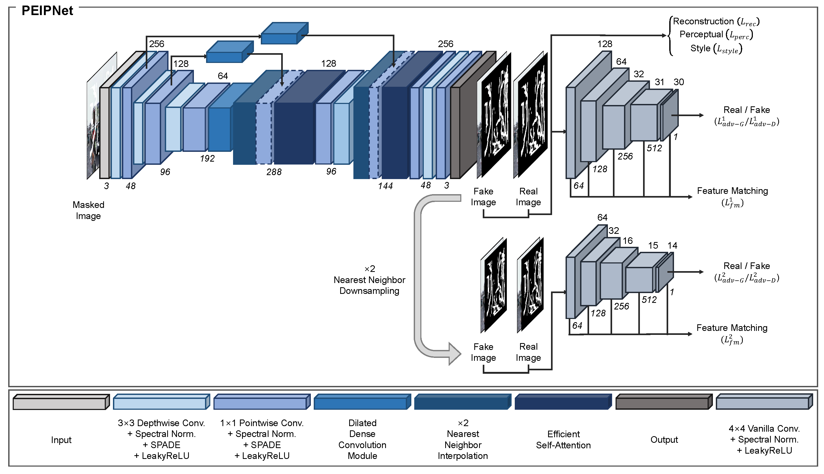
Figure 1. Structural overview of PEIPNet model.
Preprints 83884 g001
Figure 2. Structural overview of spatially-adaptive denormalization (SPADE).
Preprints 83884 g002
Figure 3. Structural overview of dense dilated convolution module (DDCM).
Preprints 83884 g003
Figure 4. Structural overview and comparison of dot-product self-attention and efficient self-attention (ESA).
Preprints 83884 g004
Figure 5. Qualitative results of our method and other models on the Paris StreetView dataset. From left to right: (a) input masked images, (b) EC [24], (c) RFR [62], (d) CTSDG [64], I SPL [65], (f) ours, and (g) ground-truth images.
Preprints 83884 g005
Figure 6. Qualitative results of our method and other models on the CelebA dataset. From left to right: (a) input masked images, (b) EC [24], (c) RFR [62], (d) CTSDG [64], (e) SPL [65], (f) ours, and (g) ground-truth images.
Preprints 83884 g006
Figure 7. Qualitative results of our method and other models on the Places2 dataset. From left to right: (a) input masked images, (b) EC [24], (c) CTSDG [64], (d) CR-Fill [63], (e) SPL [65], (f) ours, and (g) ground-truth images.
Preprints 83884 g007
Figure 8. Qualitative comparisons of ablation experiments on the Paris StreetView dataset with different combinations of proposed DDCM and ESA. DC, DB, and ESA denote dilated convolution, dense block, and efficient self-attention, respectively. O and X are the occupancy of the corresponding module.
Preprints 83884 g008
Table 1. Number of parameters and complexities of compared methods. Our result is highlighted as bold.
Method Number of Model Parameters Operational Memory ( M i B ) Parameter Difference Ratio
EC 21,535,684 2,291.2 23.91
RFR 31,224,064 2,119.5 34.66
CR-Fill 4,052,478 2,075.5 4.50
CTSDG 52,147,787 2,118.2 57.89
SPL 45,595,431 2,107.5 50.61
Ours 900,875 301.4 1
Table 2. Quantitative comparisons over the Paris StreetView dataset with different mask rates between EC, RFR, CTSDG, SPL, and our method. ↓ indicates lower is better and ↑ indicates higher is better. The best result is highlighted as bold and the second-best result is marked with underline.
Dataset Paris Streetview
Mask Ratio (0.1,0.2] (0.2,0.3] (0.3,0.4] (0.4,0.5]
FID (↓) EC 18.5194 29.1657 41.9956 57.1491
RFR 16.6533 24.3895 34.3220 47.7101
CTSDG 18.8494 30.4578 46.1283 63.7335
SPL 17.7120 28.6431 44.2332 58.4954
Ours 14.8024 23.5567 38.1458 54.1898
LPIPS (↓) EC 0.0375 0.0663 0.102 0.1479
RFR 0.0337 0.0598 0.0896 0.1302
CTSDG 0.0373 0.0693 0.11 0.1606
SPL 0.0367 0.068 0.1084 0.1571
Ours 0.0301 0.0559 0.0943 0.1428
SSIM (↑) EC 0.9397 0.8946 0.8405 0.7764
RFR 0.9468 0.9052 0.8533 0.7911
CTSDG 0.9471 0.9035 0.8469 0.7826
SPL 0.9578 0.923 0.877 0.8209
Ours 0.9522 0.9123 0.8605 0.8012
PSNR (↑) EC 30.9867 28.1855 25.749 23.8551
RFR 31.76 28.866 26.2591 24.4081
CTSDG 31.8254 28.8162 26.0823 24.2014
SPL 33.3091 30.226 27.3961 25.5072
Ours 32.4553 29.4006 26.6137 24.7842
Table 3. Quantitative comparisons over the CelebA dataset with different mask rates between EC, RFR, CTSDG, SPL, and our method. ↓ denotes lower is better, and ↑ indicates higher is better. The best result is highlighted as bold and the second-best result is marked with underline.
Dataset CelebA
Mask Ratio (0.1,0.2] (0.2,0.3] (0.3,0.4] (0.4,0.5]
FID (↓) EC 2.0626 2.8117 4.0842 6.0656
RFR 3.2892 4.8099 6.9820 9.8065
CTSDG 3.9021 6.7093 10.5437 15.1646
SPL 2.2515 3.1305 4.5734 6.3852
Ours 2.3552 3.1706 4.6410 7.1648
LPIPS (↓) EC 0.026 0.0468 0.0721 0.1032
RFR 0.0232 0.0416 0.0641 0.0908
CTSDG 0.0293 0.0551 0.0858 0.1208
SPL 0.0359 0.0578 0.0839 0.1142
Ours 0.0195 0.0385 0.0638 0.0962
SSIM (↑) EC 0.952 0.9148 0.8712 0.821
RFR 0.9583 0.923 0.8813 0.834
CTSDG 0.9533 0.9146 0.8697 0.8199
SPL 0.9632 0.9358 0.9022 0.8624
Ours 0.9613 0.9285 0.8892 0.8445
PSNR (↑) EC 32.0645 28.6826 26.1033 24.0045
RFR 32.8072 29.2923 26.6869 24.6201
CTSDG 31.996 28.4897 25.9326 23.9307
SPL 33.7915 30.611 28.0283 25.8719
Ours 33.356 29.7005 26.9822 24.8199
Table 4. Quantitative comparisons on the Places2 dataset with different mask rates between EC, CTSDG, CR-Fill, SPL, and our method. ↓ denotes lower is better and ↑ indicates higher is better. The best result is highlighted as bold and the second-best result is marked with underline.
Dataset Places2
Mask Ratio (0.1,0.2] (0.2,0.3] (0.3,0.4] (0.4,0.5]
FID (↓) EC 1.4810 3.3814 6.2819 10.7867
CTSDG 1.1672 3.3474 7.3858 14.0385
CR-Fill 0.9558 2.2416 4.3691 7.7783
SPL 0.6680 1.8749 4.0821 7.7864
Ours 0.6796 1.9225 4.8417 10.5155
LPIPS (↓) EC 0.0515 0.0897 0.1323 0.1804
CTSDG 0.048 0.0925 0.1444 0.2021
CR-Fill 0.0444 0.0808 0.1219 0.1689
SPL 0.0373 0.0726 0.114 0.1618
Ours 0.0365 0.0709 0.1139 0.1657
SSIM (↑) EC 0.9225 0.8654 0.8039 0.737
CTSDG 0.935 0.8795 0.8186 0.7522
CR-Fill 0.9325 0.8784 0.8193 0.7542
SPL 0.9547 0.9128 0.8643 0.8089
Ours 0.9419 0.8929 0.8378 0.777
PSNR (↑) EC 27.9966 24.9664 22.826 21.1286
CTSDG 29.0271 25.6747 23.3848 21.6154
CR-Fill 28.5685 25.1761 22.8066 20.95
SPL 31.2566 27.7344 25.2727 23.3253
Ours 29.8566 26.4925 24.1477 22.3093
Table 5. Quantitative comparisons of ablation experiments over the Paris StreetView dataset with different combinations of proposed DDCM and ESA. ↓ denotes lower is better and ↑ indicates higher is better. The best result is highlighted as bold.
Dataset Paris Streetview
DDCM ESA Average
FID
(↓)
Average
LPIPS
(↓)
Average
SSIM
(↑)
Average
PSNR
(↑)
Dilated Conv. Dense Block
42.6749 0.1005 0.8690 27.5524
41.1195 0.0971 0.8713 27.6425
40.8669 0.0971 0.8717 27.6685
39.8682 0.0963 0.8740 27.7794
39.4503 0.0920 0.8737 27.8604
38.8718 0.0911 0.8745 27.9010
38.0788 0.0903 0.8771 28.0407
35.7588 0.0869 0.8796 28.1083
Table 6. Number of parameters and complexities of different combinations of proposed DDCM and ESA.
DDCM ESA Number of
Model Parameters
Operational
Memory
Dilated Conv. Dense Block
418,763 286.1
695,243 300.9
624,395 287.4
900,875 301.2
418,763 287
695,243 300.8
624,395 287.8
900,875 301.4
Disclaimer/Publisher’s Note: The statements, opinions and data contained in all publications are solely those of the individual author(s) and contributor(s) and not of MDPI and/or the editor(s). MDPI and/or the editor(s) disclaim responsibility for any injury to people or property resulting from any ideas, methods, instructions or products referred to in the content.
Copyright: This open access article is published under a Creative Commons CC BY 4.0 license, which permit the free download, distribution, and reuse, provided that the author and preprint are cited in any reuse.
Prerpints.org logo

Preprints.org is a free preprint server supported by MDPI in Basel, Switzerland.

Subscribe

© 2024 MDPI (Basel, Switzerland) unless otherwise stated