Machine Learning–Based Regression Models for Steel Furnace Automation

Preprint

Article

Machine Learning–Based Regression Models for Steel Furnace Automation

This version is not peer-reviewed.

This version is not peer-reviewed.

Altmetrics

Downloads

128

Views

Comments

Submitted:

04 September 2023

Posted:

05 September 2023

You are already at the latest version

A peer-reviewed article of this preprint also exists.

Abstract

Computational Fluid Dynamics (CFD)-based simulation has been the traditional way to model complex industrial systems and processes. One very large and complex industrial system that has benefited from CFD-based simulations is the steel blast furnace. The problem with the CFD-based simulation approach is that it tends to be very slow to generate data. The CFD-only approach may not be fast enough for use in real-time decision-making. To address this issue, in this work, the authors propose the use of machine learning techniques to train and test models based on data generated via CFD simulation. Regression models based on neural networks are compared to tree boosting models. In particular, several areas (tuyere, raceway, and shaft) of the blast furnace are modeled using these approaches. The results of the model training and testing are presented and discussed. The obtained R2 metrics are, in general, very high. The results look promising and may help to improve the efficiency of operator and process engineer decision-making when running a blast furnace.

Keywords:

Subject:

Engineering - Industrial and Manufacturing Engineering

1. Introduction

The ironmaking blast furnace is a countercurrent chemical reactor designed to drive high-temperature CO- and H₂-reducing gases through a packed bed of burden material. The burden is made up of iron oxides and coke (carbon) fuel. The hot reducing gas, generated via the combustion of fuels and oxygen-enriched hot blast air delivered through nozzles called tuyeres in the lower part of the furnace, serves to reduce the oxides into metallic iron before melting it into liquid. This liquid pig iron collects in the hearth and can then be cast and transferred to other stages of the steelmaking process. This process is responsible for most new iron production in North America, accounting for 72% of ironmaking in 2020 and a significant majority of steelmaking worldwide [1]. A wide range of operating parameters determine the performance of the blast furnace process, presenting challenges to operators in maintaining stability and reducing coke consumption (generally the most expensive fuel and responsible for a large majority of the furnace’s CO₂ emissions).

Key to this effort is maintaining process stability by selecting the proper operating conditions. One of the most critical guiding metrics in this regard is referred to as the operating window, often defined by the minimum safe temperatures of the furnace top gas and the temperature of combustion gases in the furnace raceway. Top gas temperature must be maintained above 100°C to avoid the condensation of water vapor, and raceway flame temperatures must be high enough to supply thermal energy for both reduction reactions and melting (generally over 1,800°C for North American operations). The operating parameters influencing these two variables are inversely correlated, and those which increase flame temperature generally decrease top gas temperature, and vice versa. As a result, understanding in advance the expected position of the furnace within this window for a given set of conditions is critical for operators. Other important parameters include total furnace pressure drop and gas use rates, among others.

With these parameters in mind, and understanding that even small improvements to coke consumption rates can significantly affect operating costs and CO₂ emissions, operators have turned to modeling methods for predicting the performances of their furnaces under various operating conditions. These conditions include industrial rules of thumb established over decades of experience and experimentation, heat and mass balance models designed to provide theoretical estimations [2], and the most recent addition to these tools, computational fluid dynamics (CFD) simulation. Simulation and modeling approaches provide faster and more flexible results than experimental testing, but CFD can also account for additional physical detail compared with conservation calculation approaches, including handling competing reaction rates, combustion kinetics, and the effects of fluid flow patterns.

Unfortunately, CFD-based simulation approaches generally require significant computing time for each new solution generated, with results and data generated too slowly for use in real-time or on-the-fly decision-making. To address this issue, in this work, the authors propose the use of machine learning techniques to train and test reduced-order models based on data generated via CFD simulation. In particular, several areas of the blast furnace, each corresponding to a specific phenomenological region of the process, are modeled separately using these approaches. A CFD model of each of these areas predicted phenomena under different operating conditions, with results subsequently used to train machine learning–based regression models. Regression models based on neural networks are compared with tree boosting models, and the results of the model training and testing are presented and discussed. The obtained

R^{2}

metrics are, in general, very high. The results look promising and may help to improve the efficiency in decision-making when running a steel blast furnace . Two approaches were used for the modeling. One approach used neural network–based architectures, and the other one used XGBoost. The results looked promising for both approaches. In the end, both models provided advantages and disadvantages. The XGBoost models are more accurate for within range data than the neural network models. However, XGBoost techniques do not perform well in attempts to extrapolate outside range values. For the case of extrapolation, neural networks seem to perform much better. Extrapolation to outside range output prediction is desirable for this study, and as such, both approaches are used.

R^{2}

metrics were used to measure the performance of regression models. Additionally, correlation coefficient matrices were also used to visualize the importance of the features in predicting the output values.

2. Literature Review

2.1. Regression Modeling

In statistics, the question of how well a model performs for the data is sometimes described in terms of bias and variance. In this context, bias means that the model cannot learn the true relationship in the data. For example, a linear regression cannot fit a curve. So, it has bias. Neural network–based models, for instance, can fit the training data so well that they can prove unable to adapt upon encountering new, unseen data. This is called overfitting. This difference in fitting between the train set and the test set is sometimes called the variance in the context of overfitting. So, an overfitted model on the train set may have higher variance because it does not generalize well to the test set. Therefore, the goal when building a regression model for your data is to have both good bias and variance in the context of fitting the data.

There are several approaches to fit models to regression data. Three important ones are linear regression, regression trees, and neural networks. The next sections discuss neural network–based regression and regression trees leading up to XGBoost.

2.1.1. Regression Trees

As previously indicated, regression trees can fit nonlinear data. Regression trees are a type of decision tree in which the predicted values are not discrete classes but instead are real valued numbers. The key concept here is to use the features from the samples to build a tree. The nodes in the tree are decision points leading to leaves. The leaves contain values that are used to determine the final predicted regression value.

For example, if a selected feature ranges from 0 to 255, a threshold value, such as 115, can be selected to decide which child node of the parent node should be moved to. In the simplest case, each parent node in a regression tree has two child nodes. Once the selected feature’s threshold is established, this cut off is used to help select the output regression value. In the simplest case, the child node on the left can accumulate all the output values that correspond to the values below the threshold for the given feature. Concurrently, the right node collects those above the threshold. Simply averaging values in each node can give an initial predicted value. However, this method is not the best solution. The goal in training regression trees is to try multiple thresholds and select the ones that provide the best results. Through iterative optimization and comparison of predicted values to real values, optimal regression trees can be obtained.

Regression trees start from the top and work their way down to the leaf nodes. Leaf nodes are used to select output values. Nonleaf nodes are typically decision nodes based on the optimal threshold for the range of values in that feature. The key question is how to select the optimal features to use and their optimal threshold value for a given node.

How are features and thresholds selected? One simple way is to iteratively try different thresholds and then try predicting an output value with each regression tree model candidate. For each predicted output for a given tree candidate, the approach compares the predicted value to the real value and selects the candidate that minimizes the errors. In the context of regression trees, the difference between the real and the predicted values is called the residual. This loss function is very similar to the minimum squared errors (MSE) loss function. In this case, the objective goal is to minimize these residuals.

J = \sum_{i = 1}^{n} {(r e a l_{i} - p r e d_{i})}^{2}

(1)

Given a set of output values in a node, each will be tried iteratively, and the sum of squares residual will be calculated for all the threshold candidates. Once the optimized threshold is calculated, the process can be repeated by adding new nodes. When a node can no longer be split, the process stops, and it is called a leaf. Overfitting can be an issue with regression trees. To reduce the possibility of overfitting, rules are used to stop adding nodes once some criteria have been met. As an example, if a node does not have enough samples to calculate an average, perhaps if there are less that 30 samples for this node, the nodes will stop splitting.

Another key question is the selection of features to use for the decision node. Intuitively, the process is fairly logical and simple. For each feature, the optimal threshold will be calculated as previously described. Then, of the n feature candidates, the one that minimizes the residuals will be selected.

2.1.2. AdaBoost

AdaBoost (Adaptive Boosting) is a more advanced version of the standard regression trees algorithm. In AdaBoost, trees are created with a fixed size, which are called stumps. They can be restricted to stumps of just two levels. Some stumps have more weight than others when predicting the final value. Order is important in AdaBoost. One important characteristic in AdaBoost is that errors are considered and given more importance when creating subsequent stumps.

In AdaBoost, the training samples have weights to indicate importance. As the process advances, the weights are updated. Initially, all samples have the same weight, and all weights add up to one. During training, the weight for the stump is calculated by determining the accuracy between the predicted and the real values. The stump weight is the sum of the weights of all the poorly predicted samples. The weight importance is also known as the amount of say (

w_{i m p o r t}

) and is calculated as follows:

w_{i m p o r t} = \frac{1}{2} log \frac{1 - E r r o r}{E r r o r},

(2)

where

E r r o r

represents the total number of errors.

In the next iteration, the data sample weights need to be adjusted. Samples that have caused errors in the model have their weights increased. The other samples get their weights decreased.

The formula to increase the weights for error samples is as follows:

w = w \times e^{w_{i m p o r t}} .

(3)

To decrease the weights for nonerror samples is as follows:

w = w \times e^{- w_{i m p o r t}} .

(4)

After updating the weights for the data samples, the weights are normalized to add up to 1.

In the next iteration, a new data set is created that contains more copies of the samples that have the highest error weights. These samples can be duplicated. A special random selection algorithm is used to select these samples. Although random, the algorithm favors the selection of samples with higher error weights.

Once the new training data set is created, weights are reassigned to each sample of the new data set. The new data set is the same size as the original data set. All the weights are set to be the same again, and the process begins again. The point is that penalized samples in the previous iteration are duplicated more in the new data set.

This method is how a user learns the AdaBoost stumps and their weights. Then, the user can predict with all these stumps, but the learned weights are considered when making a prediction.

2.1.3. Gradient Boost

AdaBoost, as previously described, builds small stumps with weights. Gradient boost (as compared with AdaBoost) builds subtrees that can have one node or more. But, the nodes are added iteratively. The final gradient boost tree is a linear combination of subtrees.

The first node in the linear combination of subtrees is simply one node that predicts the average of all regression outputs for the training data. The algorithm then continues additively adding subtrees. The next subtree is based on the errors from the first tree, such as the errors made in the tree that only has one node predicting the average of the y output values in the training data.

The errors are the differences between predicted and real output values. As previously described, the gradient boost tree is a linear combination of subtrees (see Equation 5). The first node predicts the average regression output, but subsequent subtrees predict residuals. These residuals are added to the initial average node and adjust the output value. The residuals are differences between predicted and real values. Similar to previously described regression trees, the residuals are assigned to nodes in the tree based on how they minimize errors.

y = s u b t r e e_{0} + l r \times s u b t r e e_{1} + l r \times s u b t r e e_{2} + l r \times s u b t r e e_{3},

(5)

where

s u b t r e e_{0}

predicts the average output, and all other subtrees predict residuals.

To prevent overfitting, a learning rate (

l r

) is assigned (which is a scaling factor) to the subtrees to control the effect of the residuals on the final regression output.

Every iteration, the new tree is used to predict new output values, and these values are compared with the real values. The difference is the residuals. These residuals are used to create the new subtree for the next iteration. Once the residuals for an iteration are calculated, a new subtree can be created. The process involves ranking the residuals. This process continues until a stopping criteria is reached. The learning rate is usually 0.1.

2.1.4. XGBoost

XGBoost [6] is an improvement on gradient boosting. It has new algorithms and approaches for creating the regression tree. It also has optimizations to improve the performance and speed by which it can learn and process data.

XGBoost has some similar characteristics to gradient boosting. The first node always predicts 0.5 instead of the average, as with gradient boosting. Also similar to gradient boosting, XGBoost fits a regression tree to calculate residuals with each subtree. Unlike gradient boosting, XGBoost has its own algorithm to build the regression tree. Formally, XGBoost [6] can be defined as follows.

For a given data set, a tree ensemble model uses K additive functions to predict the output.

{\hat{y}}_{i} = \sum_{k = 1}^{K} f_{k} (X_{i}),

(6)

where

f_{k} \in F

. The symbol F is the space of regression trees. Each

f_{k}

corresponds to an independent subtree. Each regression subtree contains an output value on each leaf. This value is represented by w. For a given sample, the decision rules in the tree are used to find the respective leaves and calculate the final prediction. This prediction is obtained by summing up the output values in the corresponding leaves. To learn the set of functions used in the regression tree, the following loss function must be minimized.

J = [\sum_{i = 1}^{n} L (y_{i}, {\hat{y}}_{i})] + \frac{1}{2} λ {(∥ w ∥)}^{2} + Υ T,

(7)

where

L (y_{i}, {\hat{y}}_{i})

is a type of MSE measuring the difference between the real and predicted values, and the term

Υ T

is used to control the number of terminal nodes. This process is called pruning, and it is part of the optimization objective. The term

\frac{1}{2} λ {(∥ w ∥)}^{2}

is a regularization parameter. It represents the output value w and helps to smooth the learned values. Also,

λ

is a scaling factor. Setting the regularization parameters to zero makes the loss become the same as the traditional gradient tree boosting.

The tree ensemble model includes functions as parameters and cannot be optimized using traditional optimization methods. Instead, the model is trained in an additive manner. Formally, let

{\hat{y}}_{i}^{(t)}

be the prediction of the instance i at iteration t. The new

f_{t}

(i.e., subtree) will need to be added to minimize the loss as follows:

J^{(t)} = [\sum_{i = 1}^{n} L (y_{i}, {\hat{y}}_{i}^{t - 1} + f_{t} (x_{i}))] + \frac{1}{2} λ {(∥ w ∥)}^{2} + Υ T .

(8)

This means that an

f_{t}

must be added greedily, which results in the most improvement to this model based on the loss. So, in XGBoost, given a node with residuals, the goal is to find output values for this node that create a subtree that minimizes the loss function. The term

\frac{1}{2} λ {(∥ w ∥)}^{2}

can be written as

\frac{1}{2} λ O_{v a l u e}^{2}

. The term

O_{v a l u e}^{2}

represents the output value.

Optimization in XGBoost is a bit different in practice from neural networks. In neural networks, derivatives are taken for gradients during the epochs in the training process, and they do back propagation. In contrast, in XGBoost, a loss has to be calculated and minimized theoretically, but in practice, the derivatives (gradients) are always the general equation of adding the residuals and dividing by the total. So, notably, no derivative calculation occurs during training. Unlike neural networks, XGBoost uses the same overall design for every single model, and the user only has to calculate the derivative once (on paper) and know that it will work for all of the models created. In contrast, every neural network has a different design (e.g., different number of hidden layers, different loss functions, different number of weights), so the user always has to calculate the gradient for each model. In general, by minimizing the loss function with the derivative, general equations are obtained, which are used to build the tree. So, this derivation gives the general formulas. This objective can be optimized in a general setting. Derivation and simplification give general equations.

In normal circumstances, it is not possible to enumerate all the possible tree structures. Instead, a greedy algorithm that starts from a single leaf and iteratively adds branches to the tree is used. As such, the process to create the tree is as follows.

In essence, different subtree candidates must be tried, and the one that optimizes the loss function should be selected. During the learning process, the tree starts with one node and tries to add more subtrees with optimal node and threshold configurations. The user needs a way to score the subtree candidates to select the best one. Each subtree gets scored using the gain value. The gain value for a subtree candidate is calculated from other values associated with each of the nodes that make up that subtree candidate. Once similarity scores for each node in the subtree candidate are obtained, they are used to calculate the gain of that particular split of the nodes in the subtree. This gain equation is used to evaluate the split candidates. For example, assuming nodes left and right for a root node, the gain can be calculated as follows:

g a i n = l e f t_s i m_s c o r e + r i g h t_s i m_s o c r e - r o o t_s i m_s c o r e .

(9)

The gain score helps to determine the correct threshold. For other threshold cutoffs, other gains can be calculated and the optimal one selected. So, the threshold that gave the largest gain is used. If a node only has one residual, then that is it, and it is a leaf.

The gain depends on similarity scores. The process to create a set of subtree candidates needs these similarity scores and is as follows. For each node in a subtree candidate, a quality score or similarity score is calculated from all the residuals in the node. The similarity score function is as follows:

s i m_s c o r e = \frac{{(s u m_o f_r e s i d u a l s)}^{2}}{n u m b e r_o f_r e s i d u a l s + λ},

(10)

where the residuals are summed first and then squared. The symbol

λ

is a regularization parameter.

Once the similarity score is calculated, the node should be split into two child nodes. The residuals are grouped into these nodes. Because the threshold for the node is not known, the feature is iteratively split from its lowest value to its highest values in the range. Here, however, XGBoost uses an optimized technique called percent quantiles to select the threshold. Residuals that belong to less than the threshold go on the left node, and residuals that belong to more than the threshold go on the right node. Once again, the similarity scores are calculated for each of the two left and right nodes.

The optimal subtree candidate is selected using the similarity score and the gain score as previously described. Once the best candidate is selected, the next step is to calculate its output values for the leaf nodes. The output values are also governed by the loss function, and the formula for them can be derived from it, as shown in Equation 11. So, for a given subtree structure, the optimal

w_{j}

of leaf j can be computed as

O_{v a l u e} = \frac{s u m_o f_r e s i d u a l s}{n u m b e r_o f_r e s i d u a l s + λ} .

(11)

This step completes the tree building process. Now, the tree can be used to predict y similarly to how this is done with gradient boosting.

y = s u b t r e e_{0} + l r \times s u b t r e e_{1} + l r \times s u b t r e e_{2} + l r \times s u b t r e e_{3},

(12)

where

s u b t r e e_{0}

predicts 0.5, and all other subtrees predict residuals that get added together but are scaled based on the learning rate

l r

2.2. Neural Networks for Regression

Neural networks can be used for regression modeling. Neural networks are universal function approximators. The function consists of an input, an output, and one or more hidden layers. They can approximate nonlinear data using activation functions such as the sigmoid function. The weights in the neural network are learned through stochastic gradient descent and back propagation. The goal is to optimize a loss function. For regression, the most common loss function is MSE.

3. Methodology

In this section, the data set, modeling methodologies, and performance metrics are presented and discussed, in addition to an overview of the CFD modeling techniques used to simulate the blast furnace process.

3.1. Computational Fluid Dynamics Modeling of the Blast Furnace

CFD modeling techniques provide unique insight into the interior state of the blast furnace, with a validated model capable of acting as a suite of soft sensors. The earliest applications of CFD to the blast furnace employed significant simplifications for physics and geometry [7,8,9], but advancements in computing capacity and technology have enabled increasingly complex modeling of combustion, heat transfer, turbulent and multiphase flow, and the other physical phenomena occurring within the furnace using real-world geometry [10,11,12]. Previous research conducted by researchers at Purdue University Northwest with validated in-house CFD solvers tailor-designed for blast furnace modeling have explored a wide range of conditions and their effects on operation, including developing guidance for fuel injection, lance design and positioning, overheat troubleshooting, and coke consumption rate reduction [13]. The modeling approach employed to generate data for this work simulates conditions within the blast furnace blowpipe and tuyere (hot blast flow and fuel injection into the furnace), raceway (fuel combustion and reducing gas generation), and shaft (chemical reduction reactions and iron melting). Full details for these models can be found in previous publications [13,14,15]. This paper will describe the core elements only in brief. Fluid flow, heat and mass transfer, and chemical reactions in all zones are simulated using the standard Navier–Stokes equations, the k-

ϵ

turbulence model, and the species transport equation, discretized with the Semi-Implicit Method for Pressure-Linked Equations scheme. The general form of the governing PDEs used are in Table 1.

Here,

ρ

is density, u is velocity,

ϕ

is the general property transported, u^t and

ϕ

^t represent the fluctuating components of velocity and the transported property owing to turbulence, and S_$ϕ$ is a source term. Y_i is the local mass fraction of species, i; R_i is the net production rate of that species;

Γ

_i is the species diffusion coefficient; and S_i is a source term for species creation. The k and

ϵ

are the turbulent kinetic energy and dissipation rate, respectively,

μ

_t is the turbulent viscosity, and C_$μ$,

σ

_k,

σ

_$ϵ$, C_{1 $ϵ$}, and C_{2 $ϵ$} are model constants defined as listed in Table 1. In total, 6 key chemical reactions are predicted in the tuyere and raceway regions, and 11 are predicted in the shaft, including gas combustion, the Bouduard reaction, indirect reduction of iron oxides by CO and H₂, and more.

3.1.1. CFD Model Validation and Case Matrix Scenarios

It should again be noted that although the capabilities of applied CFD modeling have been illuminated by the aforementioned and similar studies, even modern multicore PCs and high-performance computing clusters are not yet powerful enough to run simulations in near real time. It remains a challenge to provide this high-fidelity, simulation-based guidance to operators quickly enough for day-to-day operations. As this effort aims to develop a reduced-order model for a single blast furnace capable of providing equivalent operational predictions to CFD modeling in near real time, a CFD model of the selected site blast furnace was developed and validated against real-world operating conditions typical for North American blast furnaces. That model was then used to predict furnace performance at a preselected range of operating conditions relevant to industrial practice.

Validation was conducted against averages from a 2-week period of real-world operating conditions at a US Steel blast furnace. CFD results were compared against available data, including pressure, fuel and gas flow rates, gas temperatures, top gas analyzers, material charge records, and a daily production and coke rate estimation. Some assumptions were made in modeling to account for information not available or not recorded in real-world operation, including burden bulk porosity distribution and the moisture content of charged material. Table 2 shows the comparison between simulation predictions for the provided operating conditions and the monthly averages the 2-week operation period. Figure 1 also shows gas temperature and species distributions within the furnace. Industrial operators have confirmed that the cohesive zone shape and position holds with expectations based on cooling fluxes and furnace operation history.

The variables selected to generate the matrix of scenarios for training reduced-order models were natural gas injection rate, natural gas injection temperature, pulverized coal injection rate, H₂ injection rate, charged ore moisture content, and oxygen enrichment. The input variables have been normalized so as not to publish the specific operating conditions at the industrial furnace. All other variables at the tuyere level (including factors such as wind rate, steam injection, and ambient moisture) are held constant; however, modifications to the charged ore/coke ratio are made to account for the corresponding changes, which would be made in real-world operation with different fuel injection rates.

3.2. Regression with Neural Networks

The architecture for the neural network–based models consists of a regression function, which is the sum of a linear function and a nonlinear function

f (x)

, as described in Equation (13). The nonlinear part is a simple neural net (NN) with one hidden layer consisting of 10 neurons. The hidden layer used a sigmoid activation function. Both the inputs and outputs were scaled using standardization.

g (x) = w * x + b + f (x) .

(13)

The loss function is the standard MSE.

3.3. Regression with Neural Networks and Probability Density Function Shaping

Probability density function (PDF) shaping [3,4] is a technique that can help a neural network–based regression model to learn while taking into consideration the error distribution in the predicted data. The goal is to make sure that the histogram of the errors in the predicted data has a Gaussian distribution that is as close to a zero mean as possible and with as narrow a standard deviation as possible. In industrial processes, it is a good reliability and quality safeguard.

3.4. Regression with XGBoost

XGBoost is a tree-based gradient boosting technique that was described in the literature review. It has been shown to achieve good results on tabular and regression problems that have small amounts of data. XGBoost has been used extensively in Kaggle competitions with excellent performance. However, it does have well-known problems when dealing with cases that require extrapolation from the trained data ranges.

3.5. Data and Features

The data set [5] consisted of 894 samples, which were split into train and test sets. An 80% split was used after randomizing the data, which resulted in 715 samples for training and 179 for testing. There were eight key inputs and, at most, six outputs per each of the three reaction regions of the blast furnace represented by the CFD models (tuyere, raceway, and shaft). The CFD modeling techniques use input features directly representative of the operating conditions for the blast furnace. The list of input variables are shown at the upper section of Table 3. The CFD approach can generate a wide range of potential output data, predicted based on chemical reactions, mass and energy transfer, and fluid and solid flow within the process. Those selected for this study were identified as key output variables, which would influence the selection of operating conditions for stable production at an industrial blast furnace. The outputs include in this study are listed in the lower section of Table 3. Moreover, the full data set is available from the project repo [5].

3.6. Performance Metrics

The

R^{2}

metric is a measure of performance for regression models. Formally, it is called the coefficient of determination. It can be described as representing the proportion of the variation in the dependent variable that is predictable from the independent variable(s). For this project, the closer the

R^{2}

is to 1.0, the better.

4. Results

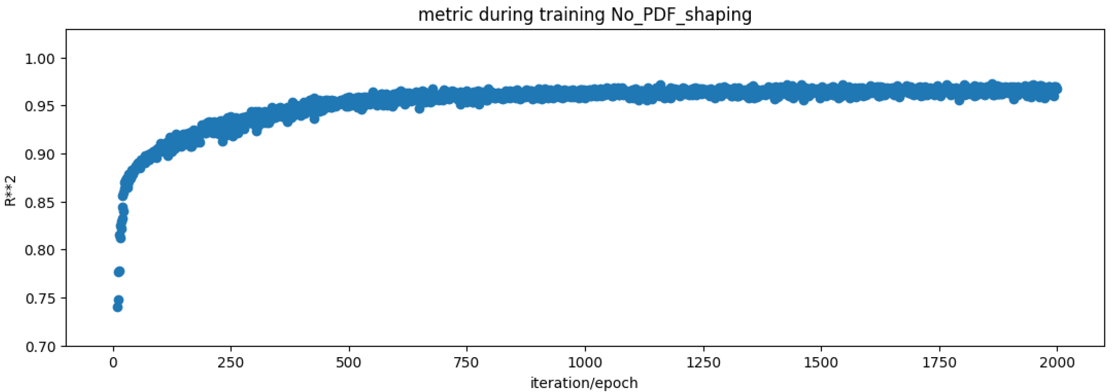
In this section, the results are presented and discussed. In general, performance was good, and the models learned quickly, as shown in the following figure.

4.1. Regression Models Comparison

This section presents a comparison of the performance across all tested models. As shown in the results, both models performed exceptionally. XGBoost and NNs in some cases had the same performance. In cases where neural nets were not able to learn, the XGBoost algorithm did best. Table 4 shows the results of multioutput models with NNs, as well as single-output models with both NNs and XGBoost. In general, it is observed that the single-output models performed slightly better than multioutput models in like-for-like comparisons. Additionally, the XGBoost algorithm showed the best performance overall (within the range of data simulated with the CFD models).

4.2. Regression Error Mappings of Predicted vs. Real Test Set

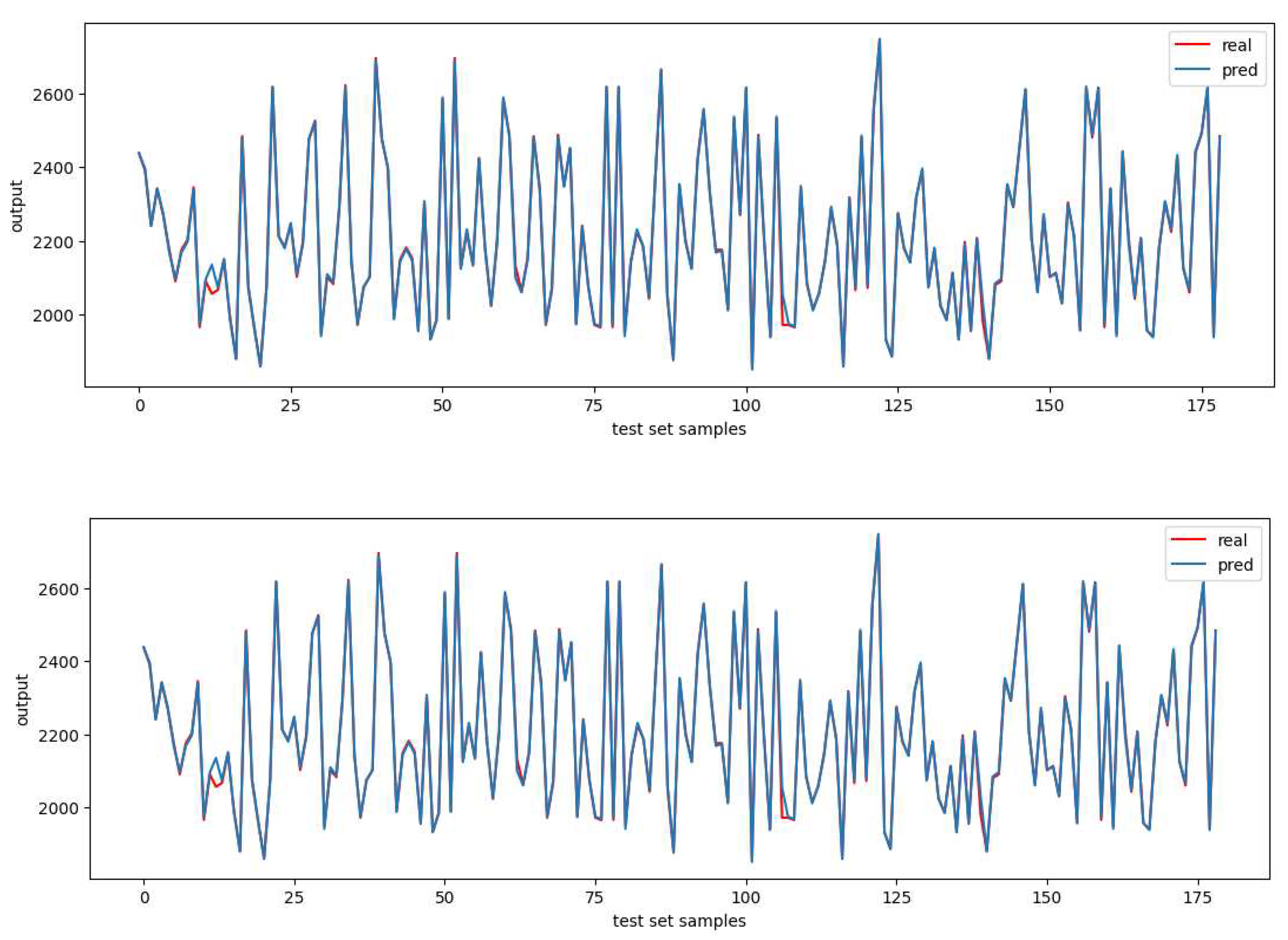
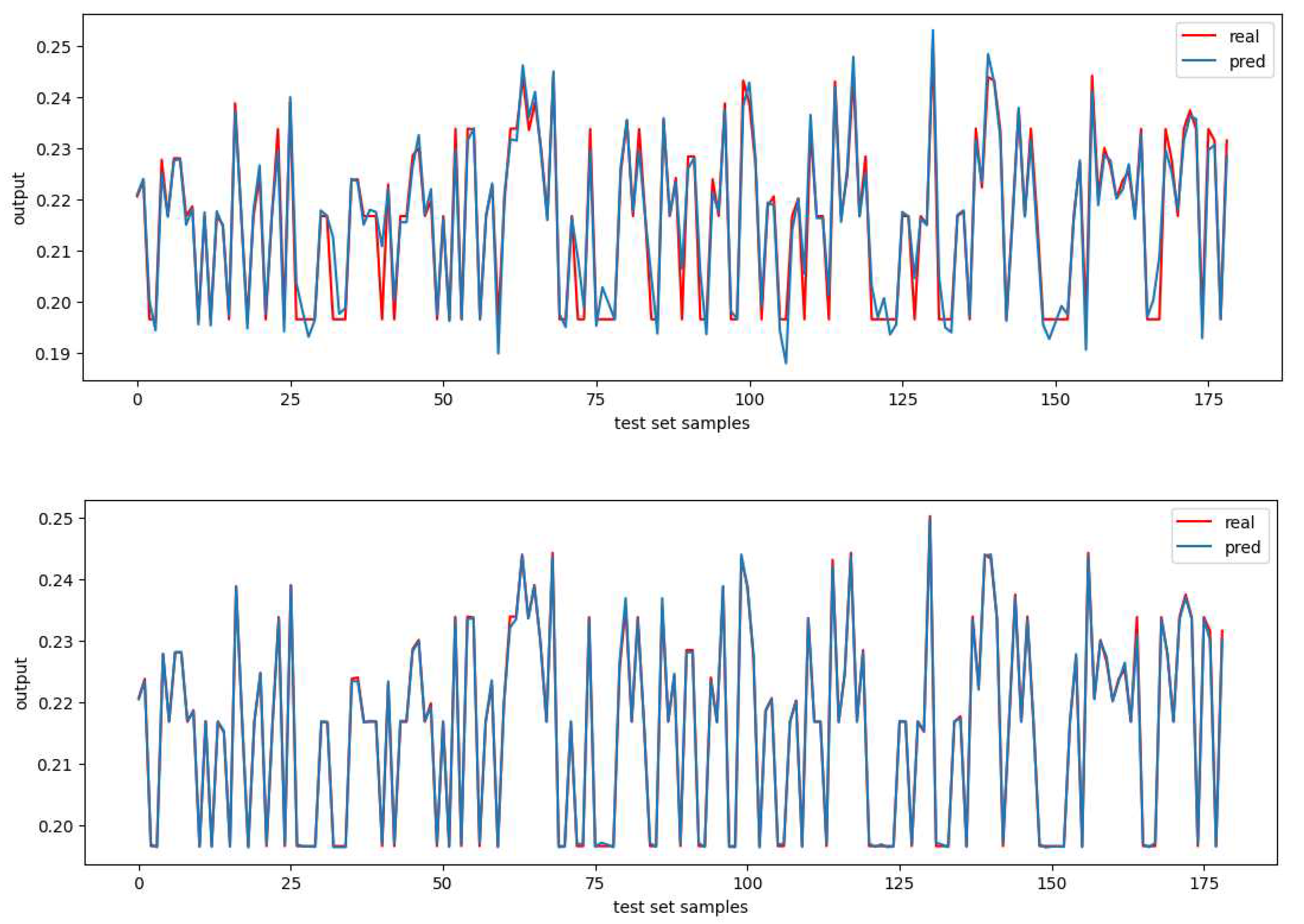
In this section, plots of the mapping between real values vs. model-predicted values are presented and discussed. Approximately 170 test samples are run by the model and compared with the real CFD-generated test samples. The results are shown in the following figures.

The figure for the raceway volume output shows that the XGBoost model fits the data better than the NN model. The figure includes two plots. The top plot shows the mapping between predicted and real values when using the neural network–based model. The bottom plot shows the mapping between predicted and real values when using the XGBoost-based model. For this case, XGBoost seems to provide better results.

The following figure shows the comparison for raceway coal burn percent. The top plot shows the mapping between predicted and real values when using the neural network–based model. The bottom plot shows the mapping between predicted and real values when using the XGBoost-based model. Again, XGBoost fit the data better.

Figure 3. Raceway coal burn percent mapping: (upper) NN, (lower) XGBoost.

Finally, the following figure shows the comparison for raceway flame temperature in kelvin between XGBoost and the NNs. In this case, it is a bit more difficult to notice the difference.

Figure 4. Raceway flame temperature in kelvin mapping: (upper) NN, (lower) XGBoost.

4.3. Regression Error Distribution Analysis for the Test Set

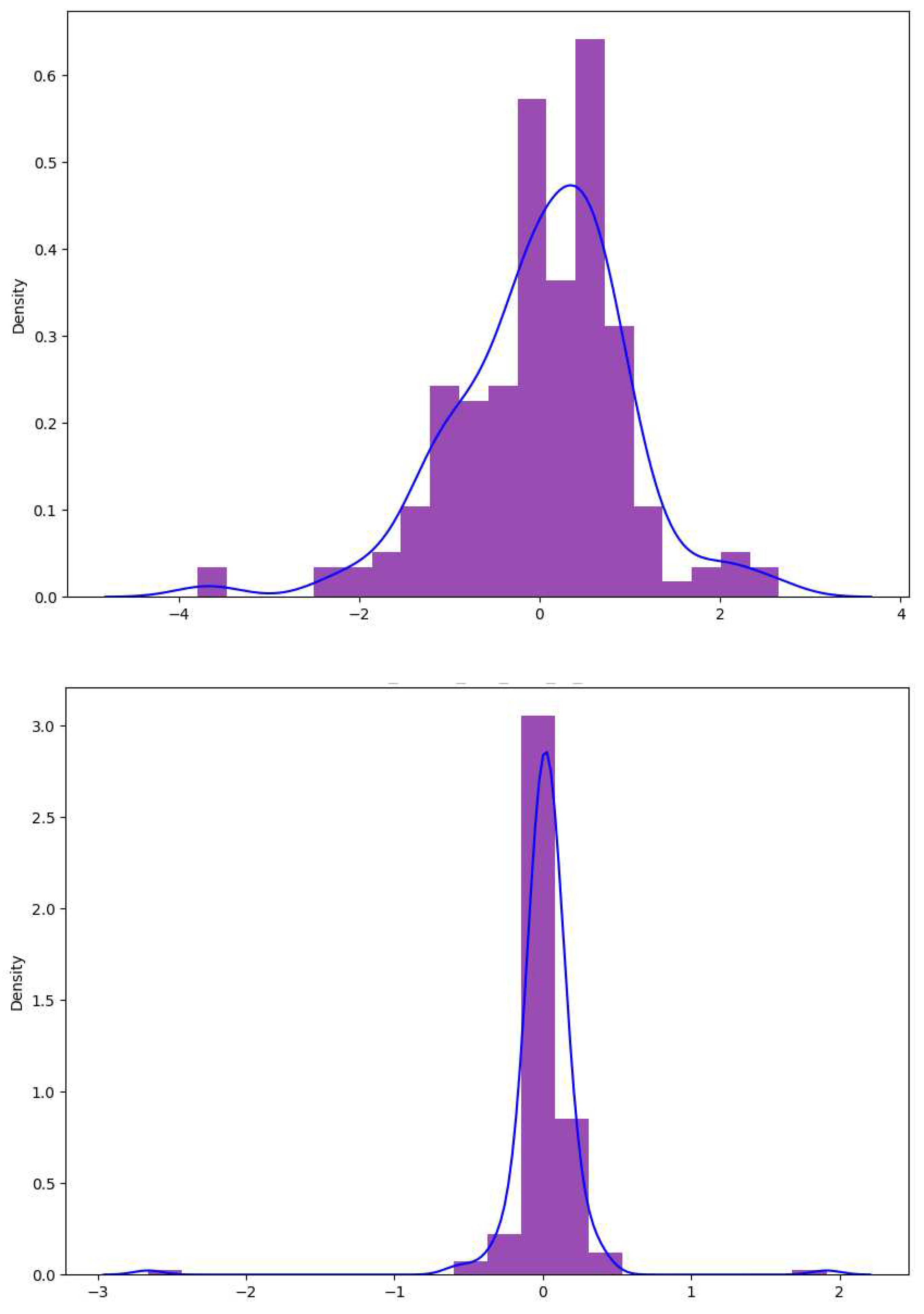
In this section, an analysis of the error distributions is performed. This section shows the comparison for tuyere exit velocity in meters per second. In general, XGBoost seems to fit a model with a predicted error PDF with zero mean and very narrow standard deviation. In contrast, the neural network model seems to have a broader standard deviation.

Figure 5. Tuyere exit velocity in meters per second: (upper) NN, (lower) XGBoost.

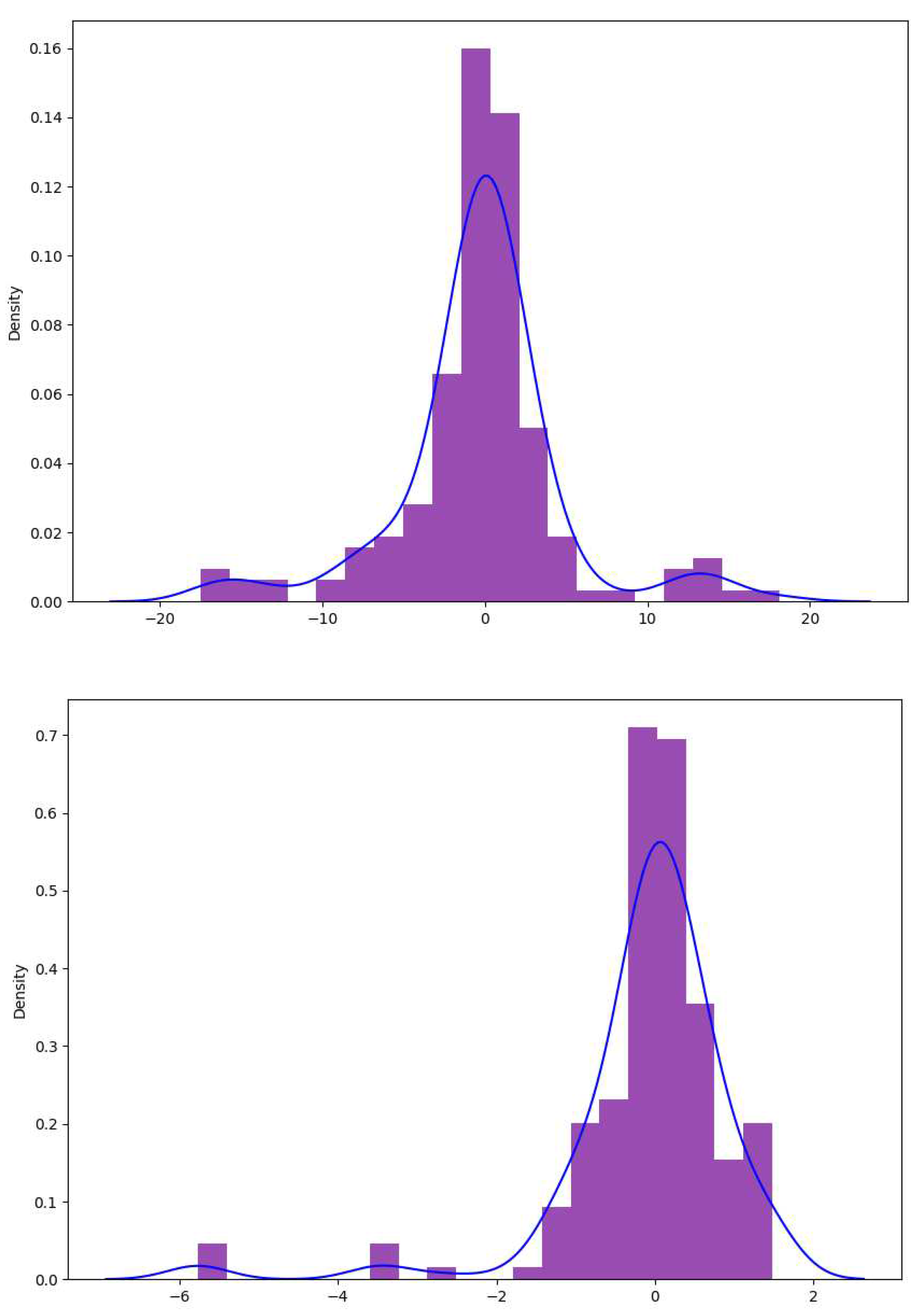
The following figure shows the comparison for tuyere

t k

, which is similar to the previous case. Although the standard deviation can vary, in general, the errors always had a PDF with zero mean.

Figure 6. (Upper) NN, (lower) XGBoost.

4.4. Correlations Matrix Analysis

It is a relatively simple matter to extract correlation coefficients between the parameters included in the physics-based modeling data. This section presents the correlation coefficient matrices as a means of analyzing the relationship between input and output variables relevant to blast furnace operation. Correlation coefficient matrices are independent of the model used and help to identify which inputs have the highest contribution to the quality of the predictive model. Additionally, for the specific scenario of examining blast furnace operation, these correlations can be compared with existing rules of thumb established by blast furnace operators over decades of operation to build confidence in the validity of the models [16].

The correlation coefficients for tuyere exit velocity are explored in Figure 7. Of the parameters considered in this study, increased tuyere exit velocity is most strongly correlated with increased natural gas injection rates, increased natural gas injection temperature, and increased H₂ injection rates. Increased gas injection rates (natural gas and hydrogen gas) result in higher gas volume and higher tuyere exit velocity. Increased natural gas injection temperature, supplied by preheating the injected gas, would also result in lower-density, higher-volume gas, necessitating increased velocity. It is observed that increasing pulverized coal injection in the tuyere results in a decline in tuyere exit velocity. This result is because the blast air must accelerate the comparably much slower stream of coal particles, losing momentum in the process.

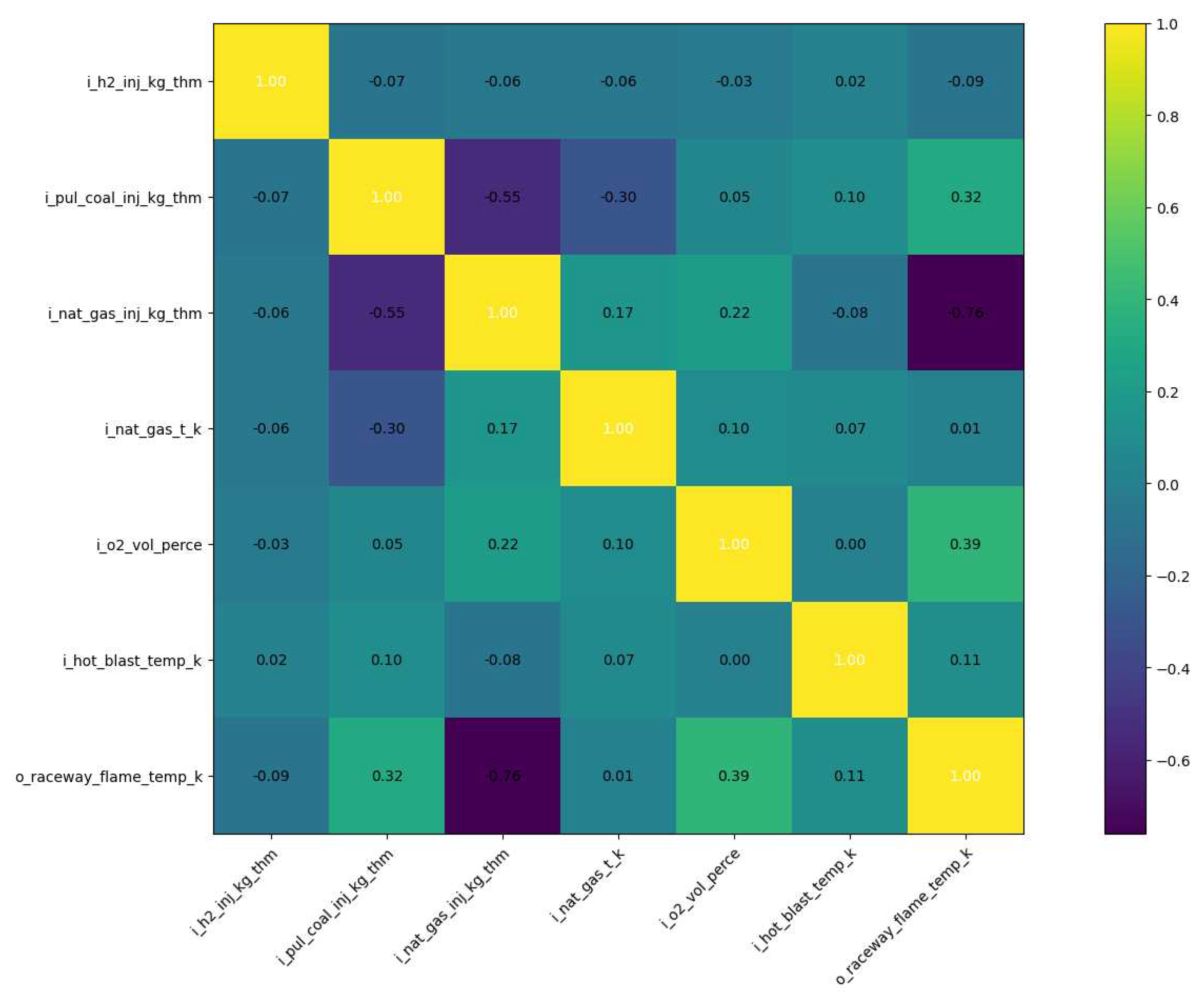
Similarly, the correlation coefficients for CFD-predicted blast furnace raceway flame temperature are detailed in Figure 8. Key parameters positively influencing the temperature of gas generated by combustion in this lower region of the furnace are pulverized coal injection, oxygen enrichment, and hot blast temperature. These parameters makes physical sense, as increasing available carbon fuel, oxygen, and sensible heat results in higher total gas temperatures after the reactions are complete. The natural gas injection rate is inversely (strongly) correlated with this flame temperature value. This result is primarily because natural gas combusts to produce CO₂ and H₂O gas, both of which participate in endothermic reactions with carbon coke, consuming heat to produce CO and H₂. This reaction results in lower total gas temperatures when injecting high levels of natural gas.

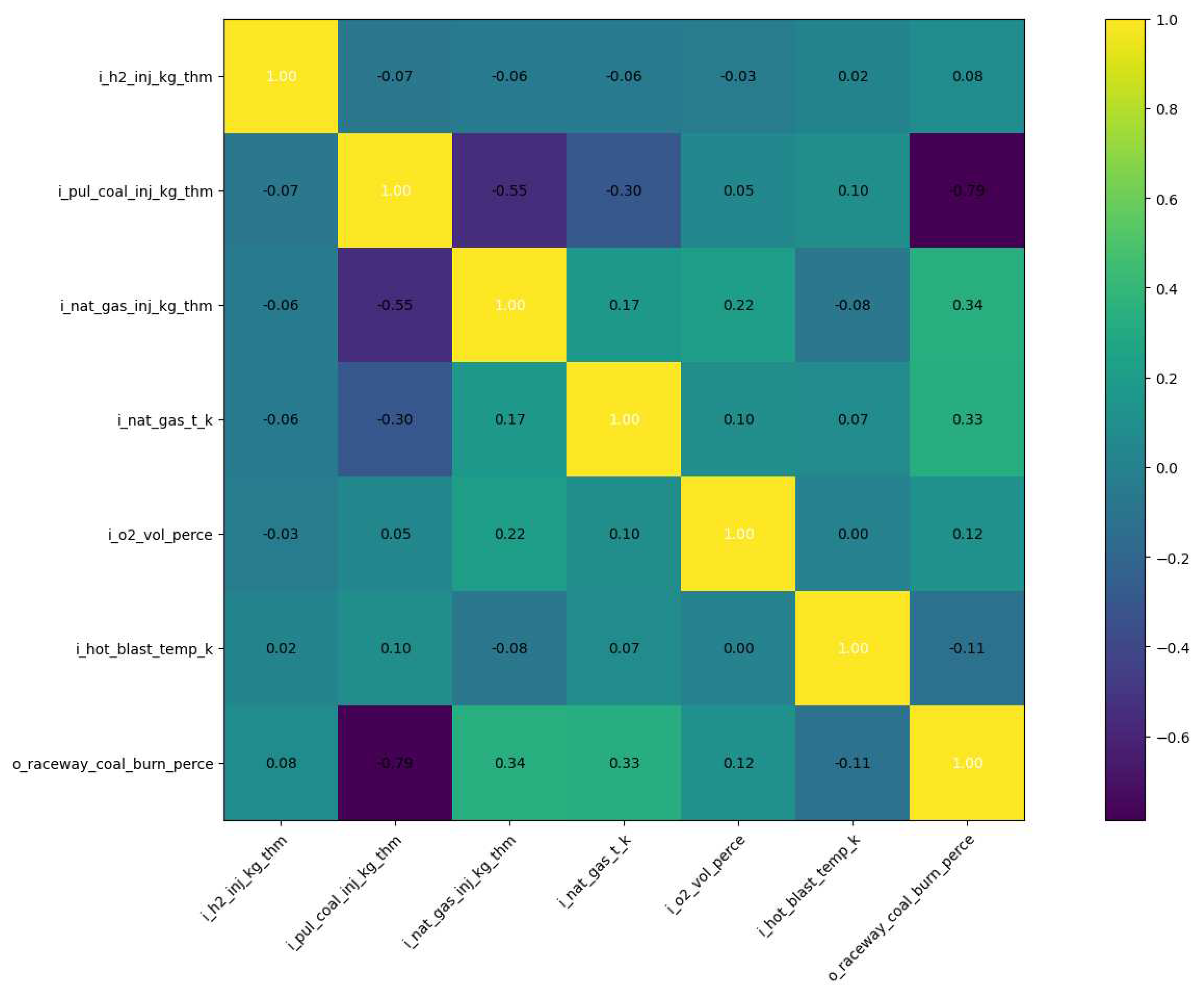
As a final example, the correlation coefficients for pulverized coal burnout (Figure 9) indicate that coal burnout is most strongly correlated (inversely) with coal injection rate. Because the rate of coal combustion is most strongly limited by the heating of the coal, the delivery of pulverized coal at high rates can results in low overall burnout. Not enough oxygen is available to combust the coal outside the raceway, so heating the particles to combustion temperatures quickly before they affect the coke bed is crucial to combustion efficiency. Increases in natural gas injection rate, natural gas temperature, and oxygen enrichment result in increased pulverized coal burnout for the same reason because each of these variables increases the rate at which pulverized coal is heated and engages combustion more rapidly.

5. Discussion

Notably, XGBoost is effective for this type of problem, but XGBoost models do not perform well in extrapolation. In general, the neural network–based models provide more-realistic predictions for data outside the training ranges, and as such, provide the more robust option for operators to utilize between the compared models discussed here. Additionally, using both models together (XGBoost within the simulated range and neural network based models for extrapolation) makes sense for this use case and probably for other industrial applications where both precision and the ability to extrapolate and predict for never-before-seen cases are desired.

6. Conclusions

In this work, the authors have used machine learning–based techniques to model certain sections of an ironmaking blast furnace. In particular, regression models using neural networks and XGBoost have been trained and tested. Analysis based on

R^{2}

statistics shows that the models perform well in the prediction of physics-based data generated by CFD modeling of the blast furnace process. Comparison with validated CFD modeling, operational data from the blast furnace in question, and additional subject matter expert analysis have all confirmed that the results of the models appear accurate to real-world operation. It was noticed that although XGBoost sometimes achieved better results, the model shows poorer effectiveness in extrapolation. In this case, even if less accurate, a neural network model is preferred to ensure a base level of realism in the predictions beyond the data sample range.

Future work will include adding more data samples, as well as generating more specific case scenarios. Finally, the effect of including real-world blast furnace sensor data in addition to simulation modeling results in the training data set will also be explored.

Author Contributions

Conceptualization, Hong Wang and Tyamo Okosun; methodology, Ricardo Calix and Hong Wang; software, Ricardo Calix; validation, Tyamo Okosun and Orlando Ugarte; formal analysis, All Authors; data creation, Orlando Ugarte; writing—original draft preparation, Ricardo Calix; writing—review and editing, Ricardo Calix and Tyamo Okosun; visualization, Ricardo Calix; supervision, Tyamo Okosun; project administration, Tyamo Okosun; funding acquisition, Tyamo Okosun. All authors have read and agreed to the published version of the manuscript.

Institutional Review Board Statement

Not applicable.

Informed Consent Statement

Not applicable.

Data Availability Statement

The data used in this work is available on GitHub at https://github.com/rcalix1/ProbabilityDensityFunctionsFromNeuralNets.

Acknowledgments

Notice: This manuscript has been authored by UT-Battelle, LLC, under contract DE-AC05-00OR22725 with the US Department of Energy (DOE). The US government retains and the publisher, by accepting the article for publication, acknowledges that the US government retains a nonexclusive, paid-up, irrevocable, worldwide license to publish or reproduce the published form of this manuscript, or allow others to do so, for US government purposes. DOE will provide public access to these results of federally sponsored research in accordance with the DOE Public Access Plan (https://www.energy.gov/doe-public-access-plan). This research was supported by the US Department of Energy’s Office of Energy Efficiency and Renewable Energy under the Industrial Efficiency and Decarbonization Office Award Number DE-EE0009390. The authors would like to thank the members of the Steel Manufacturing Simulation and Visualization Consortium for their support of this effort. Support from staff and students at Purdue University Northwest and its Center for Innovation through Visualization and Simulation is also appreciated.

Conflicts of Interest

The authors declare no conflict of interest.

References

Steel Statistical Yearbook 2020, concise version. Available online: https://worldsteel.org/wp-content/uploads/Steel-Statistical-Yearbook-2020-concise-version.pdf (accessed on 11 August 2023).
Rist, A.; Meysson, N.; "A Dual Graphic Representation of the Blast-Furnace Mass and Heat Balances," JOM 1967, 19, 50. [CrossRef]
Wang, A.; Hong, W.; "Survey on stochastic distribution systems: A full probability density function control theory with potential applications," Optimal Control 2021, Volume 42, Issue 6, Pages 1812-1839.
Hong, W.; Chakraborty, I.; Hong, W.; Tao, G.; "Co-Optimization Scheme for the Powertrain and Exhaust Emission Control System of Hybrid Electric Vehicles Using Future Speed Prediction," in IEEE Transactions on Intelligent Vehicles 2021, vol. 6, no. 3, pp. 533-545. [CrossRef]
Data Set 2023. Available online: https://github.com/rcalix1/ProbabilityDensityFunctionsFromNeuralNets (accessed on 11 August 2023).
Chen, T.Q.; Guestrin, C.; Xgboost: A Scalable Tree Boosting System. In Proceedings of the 22nd ACM SIGKDD International Conference on Knowledge Discovery and Data Mining, and (2016) . , San Francisco, 13-17 August 2016, 785-794. [CrossRef]
Tanzil, W. B. U.; Mellor, D. G.; Burgess, J. M.; “Application of a two dimensional flow, heat transfer and chemical reaction model for process guidance and gas distribution control on Port Kembla no. 5 blast furnace.” In Proceedings of 6th international iron and steel congress, Nagoya, Japan, October 21-26, 1990.
Austin, P. R.; Nogami, H.; Yagi, J.; Mathematical Model for Blast Furnace Reaction Analysis Based on the Four Fluid Model. ISIJ Int’l 1996, 37, 748–755. [CrossRef]
Austin, P. R.; Nogami, H.; Yagi, J.; T. A Mathematical Model of Four Phase Motion and Heat Transfer in the Blast Furnace. ISIJ Int’l 1997, 37, 458–467. [CrossRef]
Guo, B.; Zulli, P.; Rogers, H.; Mathieson, J. G.; Yu, A., "Three-dimensional simulation of the combustion behavior of pulverized coal injection." In Proceedings of 5th International Symposium on Multiphase Flow, Heat Mass Transfer and Energy Conversion, Xi’an, China, July 3-6, 2005.
Yeh, C. P.; Du, S. W.; Tsai, C. H.; Yang, R. J.; Numerical Analysis of Flow and Combustion Behavior in Tuyere and Raceway of Blast Furnace Fueled with Pulverized Coal and Recycled Top Gas. Energy 2012, 42, 233–240. [CrossRef]
Babich, A.; Senk, D.; Gudenau, H. W.; An Outline of the Process. Ironmaking 2016, 180–185.
Okosun, T.; Silaen, A. K.; Zhou, C. Q.; Review on Computational Modeling and Visualization of the Ironmaking Blast Furnace at Purdue University Northwest. Steel Research Int’l 2019, 90, 1900046. [CrossRef]
Fu, D.; Numerical Simulation of Ironmaking Blast Furnace Shaft. Ph.D. Dissertation, Purdue University, West Lafayette, IN, U.S.A., May 2014.
Okosun, T.; Numerical Simulation of Combustion in the Ironmaking Blast Furnace Raceway. Ph.D. Dissertation, Purdue University, West Lafayette, IN, U.S.A., May 2018.
Geerdes, M.; Chaigneau, R.; Kurunov, I.; Lingiardi, O.; Ricketts, J.; Modern Blast Furnace IronmakingAn Introduction, 3rd. Ed., Amsterdam, The Netherlands, IOS Press, 2015, pp. 195.

Figure 1. Performance tuyere

t_{k}

Figure 1. Performance tuyere

t_{k}

Figure 2. Raceway volume error mapping: (upper) NN, (lower) XGBoost.

Figure 7. Correlation coefficient matrix for tuyere exit velocity (m/s). Input and output variables are described in Table 3.

Figure 8. Correlation coefficient matrix for raceway flame temperature. Input and output variables are described in Table 3.

Figure 9. Correlation coefficient matrix for pulverized coal burnout. Input and output variables are described in Table 3.

Table 1. CFD blast furnace model governing equations.

Cons. of mass: $ϕ = 1$
Cons. of momentum: $ϕ = v e l o c i t y$	$▽ \cdot (ρ ϕ u) = ▽ \cdot (Γ_{ϕ} ▽ ϕ) - ▽ \cdot (ρ u^{t} ϕ^{t}) + S_{ϕ}$
Cons. of energy: $ϕ = e n t h a l p y$
Species transport	$▽ \cdot (ρ u Y_{i}) = ▽ \cdot (ρ Γ_{i} ▽ Y_{i}) + R_{i} + S_{i}$
Turbulent kinetic energy	$▽ \cdot (ρ k u^{t}) = ▽ \cdot (\frac{μ_{t}}{σ_{k}} ▽ k) + 2 μ_{t} S_{i j .} S_{i j} - ρ ε$
Turbulence dissipation rate	$▽ \cdot (ρ ε u^{t}) = ▽ \cdot (\frac{μ_{t}}{σ_{ε}} ▽ ε) + C_{1 ε} \frac{ε}{k} 2 μ_{t} S_{i j .} S_{i j} - C_{2 ε} ρ \frac{ε^{2}}{k}$
Where:	$μ_{t} = C ρ v l = ρ C_{μ} \frac{k^{2}}{ε}, C_{μ} = 0.09, σ_{k} = 1.00, σ_{ε} = 1.30,$
	$C_{1 ε} = 1.44$ , and $C_{2 ε} = 1.92$

Table 2. CFD model validation for US Steel blast furnace.

	$Δ P$ (kPa)	Top gas temp. (K)	Coke rate (lb/ton of HM)	CO utilization
CFD	109	391	925	47.2
Industrial data	∼115	∼370	∼926	46.8
Difference (%)	5.6	5.9	0.06	0.85

Table 3. Input and output variables of the CFD model used in this study.

Category	Variable	Definition
Input	i_h2_inj_kg_thm	H₂ injection rate in kg per ton of hot metal
Input	i_pul_coal_inj_kg_thm	Pulverized coal injection rate in kg per ton of hot metal
Input	i_nat_gas_inj_kg_thm	Natural gas injection rate in kg per ton of hot metal
Input	i_nat_gas_t_k	Natural gas injection temperature in Kelvin
Input	i_o2_vol_perce	Blast oxygen enrichment in %
Input	i_hot_blast_temp_k	Hot blast temperature in Kelvin
Input	i_ore_moisture_weight_perce	Ore moisture content by weight in %
Input	i_ore_weight_kg	Weight of iron ore charged per layer in kg
Output	o_tuyere_exit_velo_m_s	Tuyere exit velocity in meters per second
Output	o_raceway_flame_temp_k	Raceway flame temperature in Kelvin
Output	o_raceway_coal_burn_perce	Pulverized coal burnout in %
Output	o_raceway_volume_m	Raceway volume in cubic meters
Output	o_shaft_co_utiliz	CO use in %
Output	o_shaft_H₂_utiliz	H₂ use in %
Output	o_shaft_top_gas_temp_c	Blast furnace top gas temperature in Celcius
Output	o_shaft_press_drop_pa	Shaft region pressure drop in Pascals
Output	o_shaft_coke_rate_kg_thm	Change in BF coke consumption in kg per ton of hot metal
Output	o_shaft_gasspecies_v_perc	Top gas CO, CO₂, H₂, N₂ volume %

Table 4.

R^{2}

performance.

Table 4.

R^{2}

performance.

Output	Multi- output NN	Multi- output NN-PDF	Single- output NN	Single- output NN-PDF	Single- output XGBoost
Tuyere exit velocity	0.97	0.96	0.98	0.96	0.99
Tuyere exit temp.	0.95	0.96	0.95	0.93	0.99
Raceway flame temp.	0.98	0.98	0.99	0.96	0.99
Raceway coal burn	0.83	0.68	0.89	0.86	0.99
Raceway volume	0.77	0.73	0.94	0.91	0.99
H₂ use	0.83	0.82	0.80	0.78	0.85
Top gas temp.	0.95	0.95	0.98	0.98	0.98
Shaft pressure drop	0.88	0.88	0.86	0.68	0.92
Shaft coke rate	0.98	0.98	0.98	0.96	0.99
Top gas CO vol %	0.90	0.87	0.92	0.81	0.92
Top gas CO₂ vol %	0.93	0.93	0.95	0.91	0.97

Disclaimer/Publisher’s Note: The statements, opinions and data contained in all publications are solely those of the individual author(s) and contributor(s) and not of MDPI and/or the editor(s). MDPI and/or the editor(s) disclaim responsibility for any injury to people or property resulting from any ideas, methods, instructions or products referred to in the content.

© 2023 by the authors. Licensee MDPI, Basel, Switzerland. This article is an open access article distributed under the terms and conditions of the Creative Commons Attribution (CC BY) license (http://creativecommons.org/licenses/by/4.0/).

Copyright: This open access article is published under a Creative Commons CC BY 4.0 license, which permit the free download, distribution, and reuse, provided that the author and preprint are cited in any reuse.

Alerts

MDPI Initiatives

Important Links

Choose an area of interest and we will send you notifications of new preprints at your preferred frequency.

Disclaimer

Machine Learning–Based Regression Models for Steel Furnace Automation

Abstract

Keywords:

Subject:

1. Introduction

2. Literature Review

2.1. Regression Modeling

2.1.1. Regression Trees

2.1.2. AdaBoost

2.1.3. Gradient Boost

2.1.4. XGBoost

2.2. Neural Networks for Regression

3. Methodology

3.1. Computational Fluid Dynamics Modeling of the Blast Furnace

3.1.1. CFD Model Validation and Case Matrix Scenarios

3.2. Regression with Neural Networks

3.3. Regression with Neural Networks and Probability Density Function Shaping

3.4. Regression with XGBoost

3.5. Data and Features

3.6. Performance Metrics

4. Results

4.1. Regression Models Comparison

4.2. Regression Error Mappings of Predicted vs. Real Test Set

4.3. Regression Error Distribution Analysis for the Test Set

4.4. Correlations Matrix Analysis

5. Discussion

6. Conclusions

Author Contributions

Institutional Review Board Statement

Informed Consent Statement

Data Availability Statement

Acknowledgments

Conflicts of Interest

References

MDPI Initiatives

Important Links

Subscribe