Low-cost Open Source Tool for Frugal Computer Simulation of Robotics Nonlinear Control

Preprint

Article

Low-cost Open Source Tool for Frugal Computer Simulation of Robotics Nonlinear Control

Altmetrics

Downloads

168

Views

Comments

Felipe J. Torres^*

Israel Martínez,Fabio A. Aguirre,

Mario A. Garcia-Murillo,

Antonio Balvantín-García

Diego A. Núñez

Felipe J. Torres^*

Israel Martínez,Fabio A. Aguirre,

Mario A. Garcia-Murillo,

Antonio Balvantín-García

Diego A. Núñez

This version is not peer-reviewed

Submitted:

05 September 2023

Posted:

06 September 2023

You are already at the latest version

Alerts

Abstract

Commonly, professors, students and researchers from universities around the world use software distributed under a license agreement for computer simulation purposes, which requires a computer with considerable hardware capabilities. Consequently, this implies a high cost to conduct simulations that require implementing numerical methods in all areas of engineering, particularly in the field of robotics and nonlinear control. This paper presents the design and results analysis of a low-cost and open-source frugal computer simulation tool with applications to robotic nonlinear control, for instance, for numerical simulations of manipulator robot control based on dynamic models. Using a single board minicomputer with with reduced computing power, Raspberry Pi, together with free software, GNU-Octave, trajectory tracking control simulations in the joint space of a Selective Conformal Assembly Robot Arm (SCARA) are achieved by solving a system of nonlinear differential equations, represented in matrix form, which includes the control law and the system model. The results of the proposed alternative are compared by running the same simulation code on a laptop computer using MATLAB and GNU Octave, which show minimal deviations and reasonable time complexity. Moreover, considering the frugality curve calculated for this approach, in addition to the low acquisition cost of the simulation software tool, it would allow the creation of a simulation laboratory in some universities with budgetary constraints for educational and research purposes.

Keywords:

Subject: Computer Science and Mathematics - Other

1. Introduction

The post-pandemic environment reveals a daunting picture due to the global economic crisis and an uncertain future. For instance, Tilak and Kumar [1] refer to global figures indicating that up to 25% of students struggle to be part of the learning process in the absence of digital tools. This digital transition is a process with several challenges where technology plays a decisive role, and must be integrated as a relevant tool to develop and implement different types of experiments related to Science, Technology, Engineering and Mathematics (STEM) areas [2]. Thus, an institutional perspective suggests taking advantage of all the advances in e-learning and continuing to use online tools to enhance teaching and learning [3]. Therefore, in engineering education it is especially important to train students with competencies and skills in agile mindset, curiosity, reflection (in/on action), innovation, creativity, and technological knowledge [4].

While core engineering courses may be lectured face-to-face or in a virtual way, complementary studies within a particular discipline demand laboratory experience for students. In this manner, simulation-based research or educational is a special interest to be boosted, as evidenced in Magana and Jong [5], where six articles are analyzed to identify themes across all of them, such as, (a) approaches for modeling-and-simulation-centric course design; (b) teaching practices and pedagogy for modeling and simulation implementation; and (c) evidence of learning with and about modeling and simulation practices. Moreover, a simulation-based virtual laboratory tool-theoretic model that enables students to perform pre-laboratory drill activities, enhances their practical learning experience, and boosts their school performance is proposed in [6]. An evidence-driven discussion on learning and teaching, as well as their relationship, in simulation-based programming education, is facilitated by [7]. Ka0radoğan and Karadoğan [8] describes software modules for simulation-based learning in a required undergraduate engineering Dynamics course, which provide both visual and haptic feedback to the student, and evaluate their effectiveness. The design of immersive simulation-based learning modules as an alternative active-learning method for teaching and learning fundamental concepts related to database design is presented in [9]. A review of studies of Virtual Reality (VR) simulation training in STEM is detailed in [10]. Pfaff et al. [11] introduces a framework for learning mesh-based simulations using graph neural networks to accurately predict the dynamics of a wide range of physical systems, including aerodynamics, structural mechanics, and cloth.

It is emphasized that the effect of the simulation is greatly enhanced by using recent technologies [12]. However, software tools for simulations are often licensed and require periodic fees and expensive computers with considerable hardware capabilities. This condition, in addition to the global economic crisis, means that the cost for many students and researchers to evolve simulations at home for simulation-based learning or even to equip a simulation lab at universities with a low budget is unattainable. In this regard, an emerging concept called frugal innovation (FI), which implies means and ends to do more with less for many, has gained wide acceptance among academic groups. Regarding this definition, Bhatti et al. [13] refers, ’Means and ends’ describes the component of innovation that can be a process as well as an outcome to achieve affordability. ’To do more with less’ suggests efficiency in process and outcome through the use of technology to get more from few resources in the contextually constraining environment in order to achieve adaptability. ’For many’ describes the generation of economic and social value that achieves affordability and large scale. The result of these motivations, processes and ends are frugal innovations that are affordable to consumers, adaptable to contextual circumstances and accessible to vast populations. Thus, frugal engineering applications can be found in [14,15,16].

In this way, the problem of performing computer simulations at the lowest possible cost but with an acceptable level of quality [17], has been addressed from two different perspectives, one related to open-source software (OSS) and the other to the use of open-source hardware (OSH). From the OSS perspective, Wajid et al. [18] designs a free, easily distributable, customized operating system based on Ubuntu for electrical/electronic and computer engineering; Tapaskar et al. [19] highlights the employment of OSS tools in postgraduate engineering curriculum; Lotfi et al. [20] focuses on promoting the use of OSS such as Python, GNU-Octave, Modelica, Java, and Gazebo in mechatronics and robotics engineering education, where a DC motor is considered to show the application of OSS for analysis and model simulation; Saluja et al. [21] proposes a system to provide a new approach for learning and teaching software engineering processes to graduate or post graduate students; and Park [22] develops an automatic GNU Octave code for educational purposes to calculate the response of a multibody closed chain system. Regarding the OSH perspective, several papers have focused on replacing the personal computer with a single-board minicomputer. Raikar et al. [23] suggests that Raspberry Pi (RPi) can be used for practicing most laboratory courses in the computer science engineering curriculum; Alex David et al. [24] designs a DC-motor test bench online lab through a RPi for possible applications in electrical engineering education; Fernández et al. [25] describes the development of a remote Arduino lab to support online IoT learning experimentation environments connected to RPi; Mbanisi et al. [26] analyses the limitations and potential of open-source hardware such as Arduino, RPi, and BeagleBone for use in engineering education and research; Fuentes et al. [27] uses RPi devices to encourage students to work autonomously for the practical sessions of computer organization and design courses; and Vaca et al. [28] describes the design and development of a remote laboratory based on RPi with applications in electronics and control engineering. Particular emphasis is placed on the use of simulations in robotics where some opportunities are addressed in the development and validation of open source simulation platforms [29].

Thus, in this work, the OSS and OSH perspectives are brought together to develop a low-cost computational tool using open-source hardware and software, considering a single-board minicomputer Raspberry Pi and GNU-Octave, respectively. The literature review provides basic examples of simulations separately; for this reason, the feasibility of the proposed approach is demonstrated by larger scope simulations, not only from the overview of engineering education but with applications for research, such as nonlinear control of robotic systems. In this sense, results of numerical simulations of a trajectory tracking control in the joint space of a SCARA robotic manipulator based on a dynamic model using the Euler-Lagrange formalism are presented.

The remaining is organized in this manner: Section 2 describes the general features of GNU Octave and RPi; Section 3 presents the case study; Section 4 details the algorithm used for simulations; Section 5 shows the results and comparisons; and finally, conclusions are given in Section 6.

2. Details of open-source hardware and software

2.1. Raspberry Pi

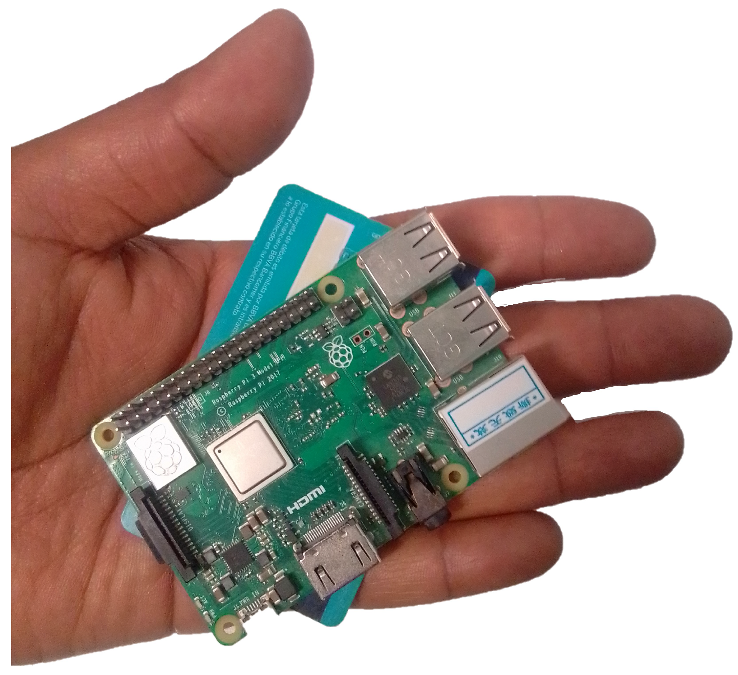
Raspberry Pi (RPi) is a single-board computer; in Figure 1, its size can be compared with that of a credit card, so it is known as a minicomputer. RPi was developed by the Raspberry Pi Foundation and first released in 2012, Raspberry Pi 2 was released in 2015, Raspberry Pi 3 was released in 2016, and Raspberry Pi 4 was released in 2019. In this work, Raspberry Pi 3 B+ has been used, with the specifications given in Table 1.

An RPi minicomputer requires an operating system to work, previously named Raspbian, but it is now called Raspberry Pi OS, which is a free operating system that is based on Debian, optimized for the Raspberry Pi hardware, and is the recommended operating system for normal use on Raspberry Pi. The OS comes with over 35000 packages, including GNU-Octave.

2.2. GNU-Octave

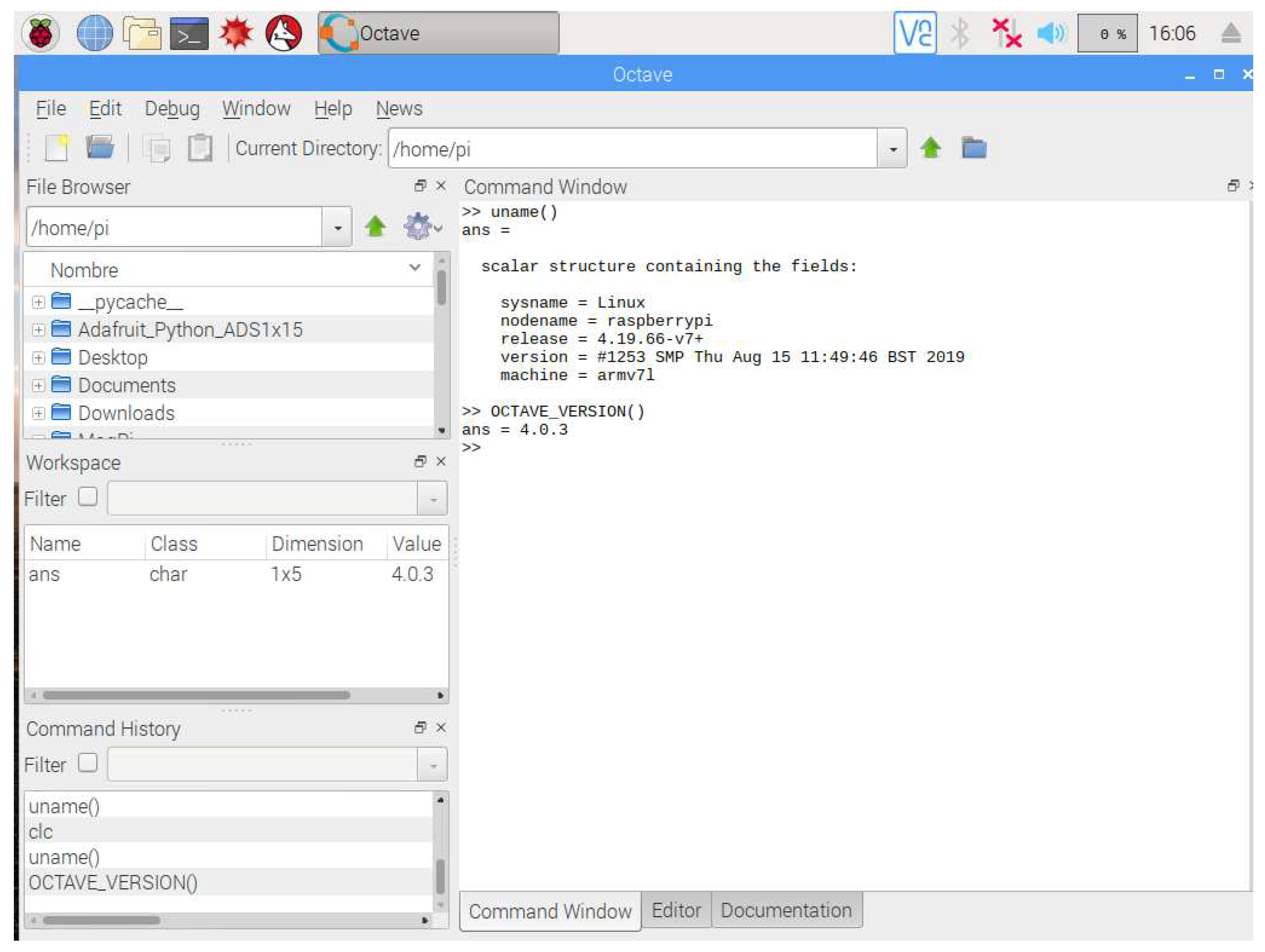
GNU-Octave is open-source and free software for numerical and scientific computing using high-level language programming. Octave is actively used for data analytics, image processing, computer vision, economic research, data mining, statistical analysis, machine learning, signal processing, and many more scientific applications [30]. Octave requires minimal hardware resources, which is a key characteristic of this work, where Octave 4.0.3 version is utilized on Raspberry Pi 3 B+ as displayed in Figure 2.

3. Case study

As part of courses on robotics, control engineering, nonlinear systems, etc., a common case of study concerns robot manipulators. The analysis first focuses on the dynamic behavior of a robot system through mathematical modeling. Then, these equations are used to develop a control law for trajectory tracking. Finally, the dynamical model and controller are entered into powerful software for simulation, probing, and research.

However, this work addresses the use of the open-source software Octave, which has a community of Octave Forge and Octave developers in a spirit of collaboration to share different packages for solving numerical computational problems. For instance, there are packages for control, communications, instrumentation, etc. that try to maintain syntax compatibility with major MATLAB^TM functions. Note that these packages include just basic functions; thus, the use of Octave for simulations of nonlinear control laws based on the dynamic system model demands the coding of algorithms for numerical approximations.

3.1. SCARA robot manipulator

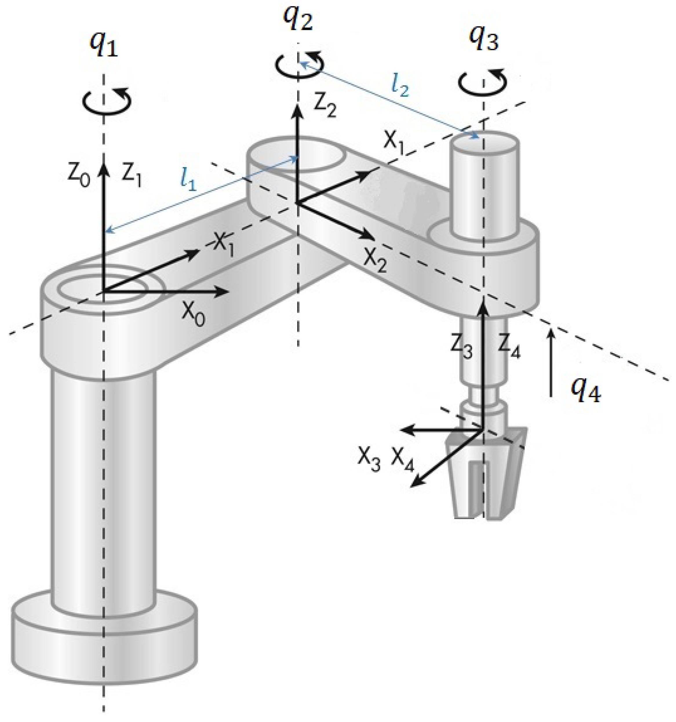
The Selective Compliant Assembly Robot Arm (SCARA) is a rigid-link system with

n = 4

degrees of freedom (dof). According to Figure 3, each joint is represented by generalized coordinated

q_{i}

i = 1, 2, \dots n

. The SCARA robot is modeled by nonlinear ordinary differential equations through Euler‒Lagrange formalism, which is expressed in matrix notation [31].

M (q_{i}) {\ddot{q}}_{i} + C (q_{i}, {\dot{q}}_{i}) {\dot{q}}_{i} + G (q_{i}) = τ_{i},

(1)

\begin{matrix} [\begin{matrix} M_{11} & M_{12} & M_{13} & M_{14} \\ M_{12} & M_{22} & M_{23} & M_{24} \\ M_{13} & M_{23} & M_{33} & M_{34} \\ M_{14} & M_{24} & M_{34} & M_{44} \end{matrix}] [\begin{matrix} {\ddot{q}}_{1} \\ {\ddot{q}}_{2} \\ {\ddot{q}}_{3} \\ {\ddot{q}}_{4} \end{matrix}] & + \end{matrix} [\begin{matrix} C_{11} & C_{12} & C_{13} & C_{14} \\ C_{12} & C_{22} & C_{23} & C_{24} \\ C_{13} & C_{23} & C_{33} & C_{34} \\ C_{14} & C_{24} & C_{34} & C_{44} \end{matrix}] [\begin{matrix} {\dot{q}}_{1} \\ {\dot{q}}_{2} \\ {\dot{q}}_{3} \\ {\dot{q}}_{4} \end{matrix}] + [\begin{matrix} 0 \\ 0 \\ 0 \\ m_{4} g \end{matrix}] = [\begin{matrix} τ_{1} \\ τ_{2} \\ τ_{3} \\ τ_{4} \end{matrix}]

(2)

\begin{matrix} M_{11} & = & I_{1} + I_{2} + I_{3} + I_{4} + m_{1} {l c_{1}}^{2} + m_{2} {l_{1}}^{2} + m_{2} [{l c_{2}}^{2} + 2 l_{1} l c_{2} c o s (q_{2})] + \\ (m_{3} + m_{4}) ({l_{1}}^{2} + {l_{2}}^{2}) + 2 l_{1} l_{2} c o s (q_{2}) \end{matrix} M_{12} = I_{2} + I_{3} + I_{4} + m_{2} [{l c_{2}}^{2} + l_{1} l c_{2} c o s (q_{2})] + (m_{3} + m_{4}) [{l_{2}}^{2} + l_{1} l_{2} c o s (q_{2})]

M13=M23=M33=I3+I4

M14=M24=M34=0

M22=I2+I3+I4+m2lc2+(m3+m4)l22

M44=m4

C11=-m2l1lc2sin(q2)q2 - (m3+m4)l1l2sin(q2)q2

C12=-m2l1lc2sin(q2)(q1+q2) - (m3+m4)l1l2sin(q2)(q1+q2)

C21= m2l1lc2sin(q2)q1 + (m3+m4)l1l2sin(q2)q1

C13=C14=C22=C23=C24=C31=C32=C33=C34=0

C41=C42=C43=C44=0

where

M (q_{i}) \in R^{n \times n}

is the inertia matrix,

C (q_{i}, {\dot{q}}_{i}) \in R^{n \times n}

is the Coriolis and centrifugal forces matrix,

G (q_{i}) \in R^{n}

is the vector of gravitational forces,

τ_{i} (t) \in R^{n}

is the vector of input torques.

I_{i}

m_{i}

l_{i}

, and

l c_{i}

are the moment of inertia, mass, final length, and the position of the mass center, for each rigid-link, respectively.

3.2. Control law for trajectory tracking

Modern control theory requires the dynamical model of the system to develop a control law. There exist diverse control strategies that have been broadly applied to robotics, such as, backstepping, sliding modes, adaptive, robust, state feedback, and more. For trajectory tracking, a computed-torque control approach which is based on Lyapunov method is implemented in this work, such as in [31,32,33]; thus, the controller is given by

τ_{i} = M (q_{i}) {\ddot{q}}_{d} + C (q_{i}, {\dot{q}}_{i}) {\dot{q}}_{d} + G (q_{i}) - k_{p} {\tilde{q}}_{i} - k_{d} {\dot{\tilde{q}}}_{i}

(3)

where

k_{p}

and

k_{d}

are positive gains,

q_{d}

is the desired trajectory, and

{\tilde{q}}_{i}

is the tracking error defined as

{\tilde{q}}_{i} = q_{i} - q_{d}

(4)

The desired trajectory for each joint is expressed by the equation:

q_{d} = q_{d i n} + \frac{q_{d f} - q_{d i n}}{2} [1 - c o s (\frac{π t}{t_{f}})]

(5)

where

q_{d i n}

and

q_{d f}

are the initial and final position of the desired trajectory, t is the time taken by the simulation step, and

t_{f}

is the total time of simulation.

The control objective is to ensure that the tracking error converges to zero in a finite time. For proving purposes, numerical approximations by means of simulations are necessary due to the analytical solutions are often abstract and complex math expressions.

4. Algorithm for simulations

The strategy of control to be applied in this case study is a closed-loop control system, it is shown in Figure 4, where the full state feedback is required in the controller (3), besides, this includes the system dynamic model that it is expressed in matrix form. In this manner, a double integration must be implemented through the coding of an algorithm for obtaining solutions, for instance, Runge-Kutta method or Euler’s method. Moreover, the code needs to work with matrix expressions and support cyclic iterations of a system of nonlinear ordinary differential equations (ODE).

4.1. Numerical ODE solver

A numerical solution of ODE with initial values is achieved using a numerical method known as solver. For instance, ode45 integrates a system of non-stiff ODE based on Runge-Kutta and Dormand-Prince methods. The general syntax of the ode45 for both MATLAB^TM and GNU-Octave is given by [34]:

[t,y]=ode45(fun,trange,init,ode_opt)

where fun is a function handle that defines the ODE of first order,

y^{'} = f (t, y)

. trange specifies the time interval over which the ODE will be evaluated. Typically, it is a two-element vector specifying the initial and final times. If there are more than two elements then the solution will also be evaluated at these intermediate time instances. init contains the initial value for the unknowns. The optional fourth argument ode_opt specifies non-default options to the ODE solver. ode45 returns two outputs, variable t is a column vector and contains the times where the solution was found, and the output y is a matrix in which each column refers to a different unknown of the problem and each row corresponds to a time in t.

In this work, the numerical simulation code has been divided into two parts, one of which is the function handle (projectileode45.m) to be integrated and the other of which is about the settings of the solver and plotting results (SCARA_inicio_ode45.m).

The pseudocode for projectileode45.m is given by:

Define name of function and output/input arguments
- Output argument will be a column vector of the derivatives
- Input arguments will be the time t and system state x
Establish the desired trajectory equations
- First and second derivative of desired trajectory are required
Set parameters values
- Parameters of the dynamical system and controller
Build matrix M and C, and vector G
Establish the controller equation
Solve dynamical equations for major order derivatives
Form the vector of derivatives to be integrated

SCARA_inicio_ode45.m pseudocode follows:

Initialize time complexity counting
Set initial values for each state variable
Specify time interval
Build ode45 solver syntax
Define desired trajectory
Plot customized figures
Stop time complexity counting

5. Results

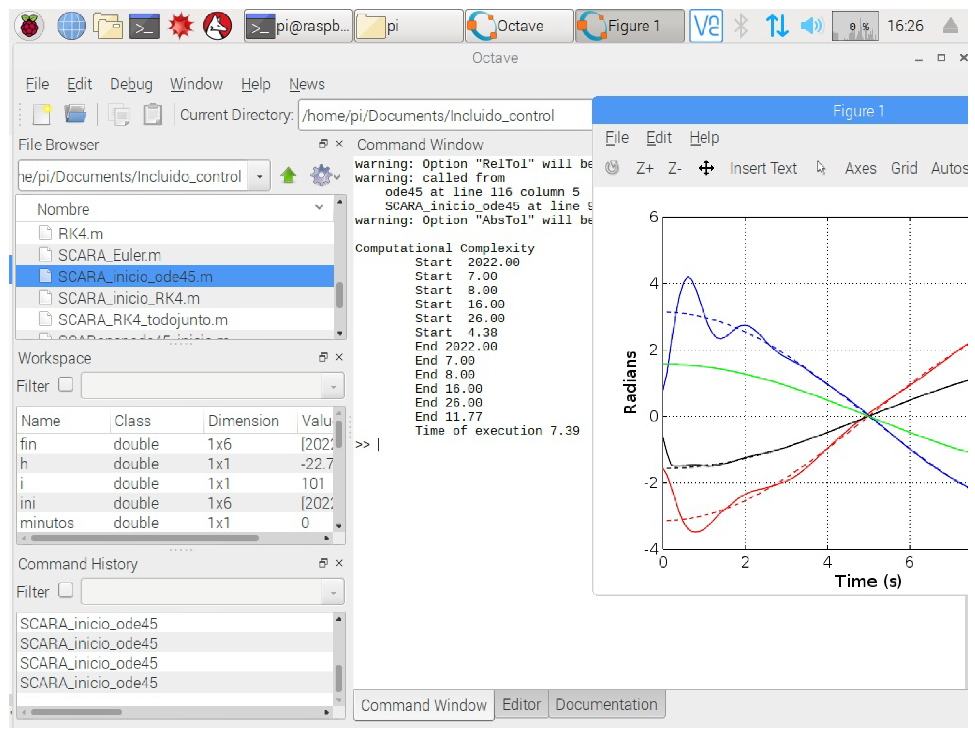
The start-up stage of the low-cost computational tool

R P i + G N U O c t a v e

is shown in Figure 5 to simulate a SCARA robot manipulator with parameters listed in Table 2.

The gains of the controller were set as

k_{p} = 50

and

k_{d} = 6

. Initial and final position for desired trajectory, as well as initial position values for each one of the joints

q_{i}

i = 1, 2, 3, 4

, are given by:

\begin{matrix} q_{d i n_{i}} & = & [- π π - \frac{π}{2} \frac{π}{2}] r a d \\ q_{d f_{i}} & = & [π - π \frac{π}{2} - \frac{π}{2}] r a d \\ q_{i} (0) & = & [- \frac{π}{2} \frac{π}{4} - \frac{π}{5} \frac{π}{2}] r a d \end{matrix}

Each one of the numerical simulation was executed on the time interval

[0 : 10]

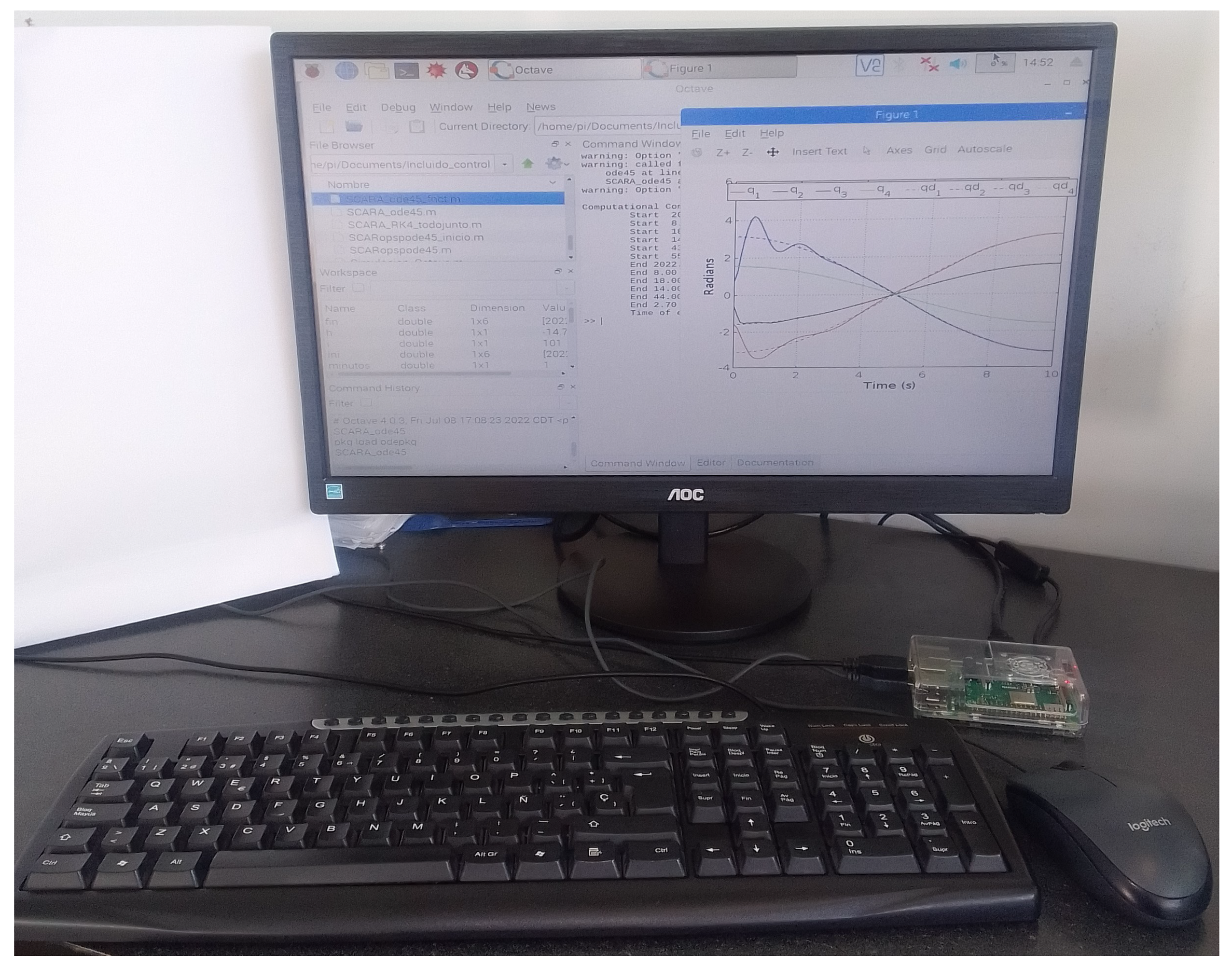
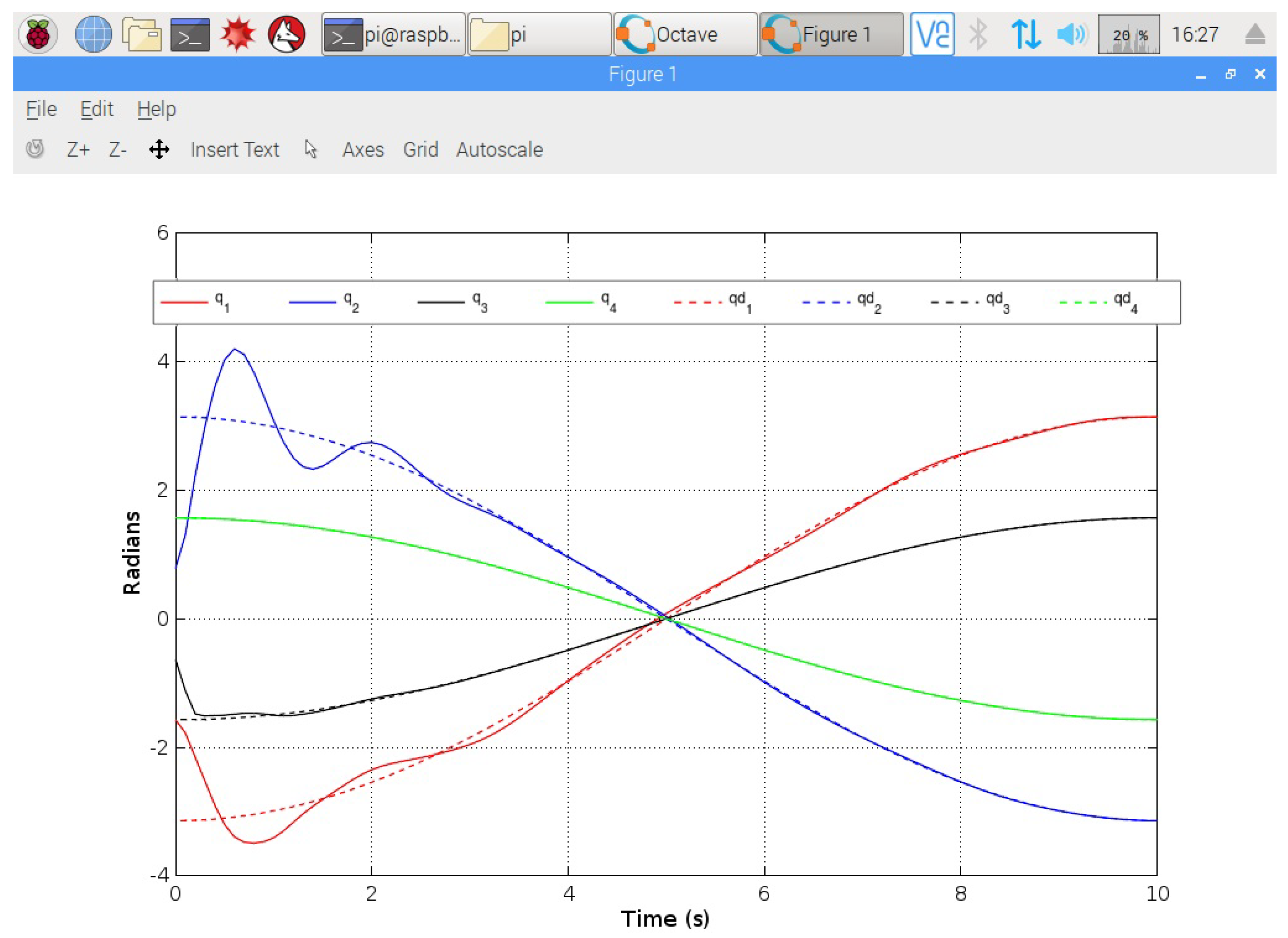
seconds. Figure 6 exhibits a screenshot of the RPi with data and graphics achieved by this proposed simulation tool. For the case study, the tracking control performance can be analyzed by the plot shown in Figure 7, where dotted lines are used for desired trajectory of each joint while solid lines are used for trajectory tracking. The controller makes the robot manipulator tracks the desired trajectory in the joint space and stay stable as time as infinity.

The same code, parameters and configurations were conducted on MATLAB^TM and GNU-Octave that were executed on a laptop computer with specifications contained in Table 3. These results are used for comparison target. Thus, plot of these simulations is like those shown in Figure 7, for this reason this figure is not included, though an analysis attending data of both solutions is set out in more detail below.

5.1. Time complexity and the standard error of the mean $α$

The time complexity caused by the numerical simulation is computed by the mean of 10 continuous executions, which is shown in Table 4.

In the simulations performed under the different software + computer schemes, it is important to demonstrate that the values of the variables obtained through the proposed tool GNU-Octave + RPi 3B+ are very close to those where the laptop is used. Table 5 shows the results of the standard error of the mean

α

(6), which is calculated for each of the variables of the case study solution, where the data of the results given by MATLAB^TM and GNU-Octave on a laptop are used as reference values.

α = \sqrt{\frac{\sum_{i = 1}^{n} {(x_{i_{r e f}} - x_{i_{R P i}})}^{2}}{n (n - 1)}},

(6)

where

x_{r e f}

is the reference value,

x_{R P i}

is the value given by the proposed tool GNU-Octave + RPi 3B+, and n is the total of values reached during the time of a numerical simulation.

5.2. Frugality score

Recently, a frugality score has been used as a parameter to measure both the consumption of computational resources and the performance of the proposed frugal innovation. In this work, a frugality score curve has been calculated based on the equations given by Sowiński et al. [14] and Evchenko et al. [35], due to the need to objectify the frugal innovation proposal and also to serve as a reference for the comparison of other similar proposals.

F r u g_{l c}^{h c} = α_{a l l} - \frac{w}{1 + \frac{1}{t_{l c} - t_{h c}}},

(7)

where

F r u g_{l c}^{h c}

is the frugality score,

l c

denotes the low-cost and open-source tool GNU-Octave + RPi 3B+, while

h c

is used to licensed software + laptop. The mean of all standard errors of the mean, shown in Table 5, is given by

α_{a l l}

, which means a measure of the numerical approximation performance. The index w defines the weight of frugality, it can vary from 0 to 1. The values of time complexity are expressed by

t_{l c}

and

t_{h c}

. With this definition of frugality, a score function is bounded within a fixed range

[- 1, α_{a l l}]

Note the importance of varying w. If

w = 0

, the frugal proposal will be weighted only by the standard errors of the mean without regard to the time complexity value. When

w = 1

, the frugality score will weight the fastest approach, i.e., the smallest difference between the time complexity values.

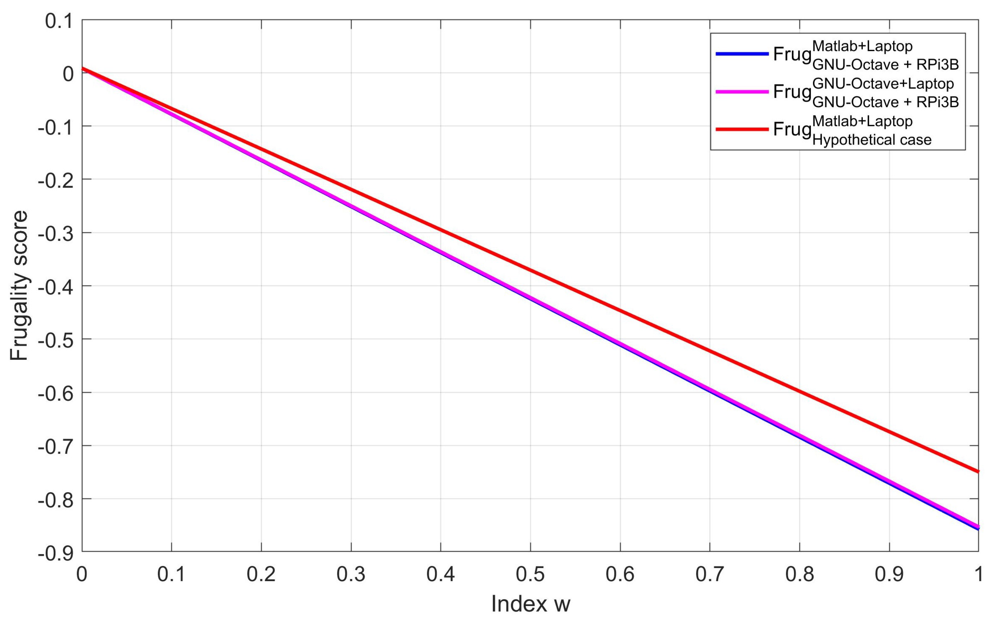
Using data from Table 4 and Table 5, frugality curves are plotted for

w = 0 : 0.1 : 1

. This is shown in Figure 8, where blue line represents frugality score of MATLAB^TM + laptop vs GNU-Octave + RPi 3B+ and red line is used for GNU-Octave + laptop vs GNU-Octave + RPi 3B+. Additionally, magenta line is a frugality curve for a hypothetical case having a time complexity of 4 seconds and the same

α_{a l l}

, which is included to demonstrate how the frugality of one proposal would be evaluated relative to another.

6. Discussion

A low-cost and open-source simulation tool for engineering has been designed and tested with results that allow its use in specific applications, such as educational applications or research on nonlinear control of robotic systems. The time complexity is compared, where the proposed tool spends 7 times more time than traditional simulation tools that utilize a laptop computer. Moreover, detailed analysis of the values of the variables given by the simulations indicates minimal differences between the simulation tool approaches. From the above, it can be said that a frugal innovation for computer simulation has been proposed.

A key criterion is the price of the hardware and software. While traditional simulation tools require a costly computer (US$669.00), a Raspberry Pi 3B+ minicomputer is cheaper (US$35.00). In addition, the cost of perpetual a MATLAB^TM license is US$2,250.00. Otherwise, GNU-Octave is free. But it is not only the low cost of the computational tool, but its ability to be affordable for most people, since it does not require learning a new programming language, so that the code used is the same as that running in licensed software widely spread in the literature.

In this manner, the proposed simulation tool has a social impact due to it is feasible for implementation in universities with a limited budget or, more individually, each student or researcher could build his or her own simulation lab at home for online education, complementary studies or research. Moreover, a frugality score is calculated to set a reference value that serves for comparison purposes with other frugal innovations of this type. Future works are intended to expand the use of GNU-Octave + RPi 3B+ for computing and simulations in connection to the internet within the focus of Society 5.0.

Author Contributions

Software and writing—original draft preparation, F.J. Torres; conceptualization and writing—review and editing, I. Martínez; methodology and validation, F.A. Aguirre; state-of-the-art and formal analysis, M.A. García; investigation, A.J. Balvantín; visualization, D.A. Núñez. All authors have read and agreed to the published version of the manuscript.

Funding

This research received no external funding.

Data Availability Statement

The data that support the findings of this study are available from the corresponding author upon reasonable request.

Conflicts of Interest

The authors declare no conflict of interest.

Abbreviations

CPU	Central Processing Unit
dof	Degrees of Freedom
FI	Frugal Innovation
GPU	Graphics Processing Unit
ODE	Ordinary Differential Equations
OSH	Open-Source Hardware
OSS	Open-Source Software
RAM	Random Access Memory
RPi	Raspberry Pi
SCARA	Selective Conformal Assembly Robot Arm
STEM	Science, Technology, Engineering and Mathematics
TM	Trade Marker
VR	Virtual Reality

References

Tilak, J.B.; Kumar, A.G. Policy Changes in Global Higher Education: What Lessons Do We Learn from the COVID-19 Pandemic? Higher Education Policy 2022, pp. 1–1.
Cardoso, A.; Oliveira, P.M.; Sá, J. Pocket Labs as a STEM Learning Tool and for Engineering Motivation. International Conference on Interactive Collaborative Learning. Springer, 2022, pp. 413–422.
Pokhrel, S.; Chhetri, R. A literature review on impact of COVID-19 pandemic on teaching and learning. Higher Education for the Future 2021, 8, 133–141. [Google Scholar] [CrossRef]
Ciolacu, M.I.; Mihailescu, B.; Rachbauer, T.; Hansen, C.; Amza, C.G.; Svasta, P. Fostering Engineering Education 4.0 Paradigm Facing the Pandemic and VUCA World. Procedia Computer Science 2023, 217, 177–186. [Google Scholar] [CrossRef]
Magana, A.J.; de Jong, T. Modeling and simulation practices in engineering education. Computer Applications in Engineering Education 2018, 26, 731–738. [Google Scholar] [CrossRef]
Altalbe, A.A. Performance impact of simulation-based virtual laboratory on engineering students: a case study of Australia virtual system. IEEE Access 2019, 7, 177387–177396. [Google Scholar] [CrossRef]
Jamil, M.G.; Isiaq, S.O. Teaching technology with technology: approaches to bridging learning and teaching gaps in simulation-based programming education. International Journal of Educational Technology in Higher Education 2019, 16, 1–21. [Google Scholar] [CrossRef]
Karadoğan, E.; Karadoğan, F. Simulation-based learning modules for undergraduate engineering dynamics. Computer Applications in Engineering Education 2019, 27, 846–862. [Google Scholar] [CrossRef]
Ozden, S.G.; Ashour, O.M.; Negahban, A. Novel simulation-based learning modules for teaching database concepts. 2020 ASEE Virtual Annual Conference Content Access, 2020.
Pellas, N.; Dengel, A.; Christopoulos, A. A scoping review of immersive virtual reality in STEM education. IEEE Transactions on Learning Technologies 2020, 13, 748–761. [Google Scholar] [CrossRef]
Pfaff, T.; Fortunato, M.; Sanchez-Gonzalez, A.; Battaglia, P.W. Learning mesh-based simulation with graph networks. arXiv 2020, arXiv:2010.03409 2020. [Google Scholar]
Chernikova, O.; Heitzmann, N.; Stadler, M.; Holzberger, D.; Seidel, T.; Fischer, F. Simulation-based learning in higher education: A meta-analysis. Review of Educational Research 2020, 90, 499–541. [Google Scholar] [CrossRef]
Bhatti, Y.; Basu, R.R.; Barron, D.; Ventresca, M.J. Frugal innovation: Models, means, methods; Cambridge University Press, 2018.
Sowiński, P.; Rachwał, K.; Danilenka, A.; Bogacka, K.; Kobus, M.; Dąbrowska, A.; Paszkiewicz, A.; Bolanowski, M.; Ganzha, M.; Paprzycki, M. Frugal Heart Rate Correction Method for Scalable Health and Safety Monitoring in Construction Sites. Sensors 2023, 23, 6464. [Google Scholar] [CrossRef]
Kwon, J.; Park, D. Hardware/software co-design for tinyml voice-recognition application on resource frugal Edge Devices. Applied Sciences 2021, 11, 11073. [Google Scholar] [CrossRef]
Sanchez, R.; Groc, M.; Vuillemin, R.; Pujo-Pay, M.; Raimbault, V. Development of a Frugal, In Situ Sensor Implementing a Ratiometric Method for Continuous Monitoring of Turbidity in Natural Waters. Sensors 2023, 23, 1897. [Google Scholar] [CrossRef] [PubMed]
Jayabalan, J.; Dorasamy, M.; Raman, M. Reshaping higher educational institutions through frugal open innovation. Journal of Open Innovation: Technology, Market, and Complexity 2021, 7, 145. [Google Scholar] [CrossRef]
Wajid, B.; Ekti, A.R.; AlShawaqfeh, M.K. Ecebuntu-an innovative and multi-purpose educational operating system for electrical and computer engineering undergraduate courses. Electrica 2018, 18, 210–217. [Google Scholar] [CrossRef]
Tapaskar, R.; Revankar, P.; Gorwar, M.; Hosmath, R. Pedagogical Interventions through Software Tools in Postgraduate Engineering Programme. Journal of Engineering Education Transformations 2018, 31. [Google Scholar]
Lotfi, N.; Auslander, D.; Rodriguez, L.A.; Mbanisi, K.C.; Berry, C.A. Use of Open-source Software in Mechatronics and Robotics Engineering Education–Part I: Model Simulation and Analysis. Computers in Education Journal 2021, 12. [Google Scholar]
Saluja, M.K.; Thakur, S. Open Source Software Based Education and Training Framework for Software Engineering Education. Solid State Technology 2020, 63, 9633–9645. [Google Scholar]
Park, Y. Development of an Educational Code of Deriving Equations of Motion and Analyzing Dynamic Characteristics of Multibody Closed Chain Systems using GNU Octave for a Beginner. Journal of Applied and Computational Mechanics 2022, 8, 232–244. [Google Scholar]
Raikar, M.M.; Desai, P.; Vijayalakshmi, M.; Narayankar, P. Upsurge of IoT (Internet of Things) in engineering education: A case study. 2018 International Conference on Advances in Computing, Communications and Informatics (ICACCI). IEEE, 2018, pp. 191–197.
Alex David, S.; Ravikumar, S.; Rizwana Parveen, A. Raspberry Pi in computer science and engineering education. In Intelligent Embedded Systems; Springer, 2018; pp. 11–16.
Fernández-Pacheco, A.; Martin, S.; Castro, M. Implementation of an Arduino remote laboratory with raspberry Pi. 2019 IEEE Global Engineering Education Conference (EDUCON). IEEE, 2019, pp. 1415–1418.
Mbanisi, K.C.; Auslander, D.M.; Berry, C.A.; Rodriguez, L.A.; Molki, M.; Lotfi, N. Promoting Open-source Hardware and Software Platforms in Mechatronics and Robotics Engineering Education. 2020 ASEE Virtual Annual Conference Content Access, 2020.
Fuentes, P.; Camarero, C.; Herreros, D.; Mateev, V.; Vallejo, F.; Martinez, C. Addressing Student Fatigue in Computer Architecture Courses. IEEE Transactions on Learning Technologies 2022. [Google Scholar] [CrossRef]
Vaca, N.; Garcia-Loro, F.; Martin, S.; Rodriguez-Artacho, M. Raspberry Pi Applications in Electronics and Control Laboratories. 2022 IEEE Global Engineering Education Conference (EDUCON). IEEE, 2022, pp. 1709–1713.
Choi, H.; Crump, C.; Duriez, C.; Elmquist, A.; Hager, G.; Han, D.; Hearl, F.; Hodgins, J.; Jain, A.; Leve, F.; others. On the use of simulation in robotics: Opportunities, challenges, and suggestions for moving forward. Proceedings of the National Academy of Sciences 2021, 118, e1907856118. [Google Scholar] [CrossRef]
Pajankar, A.; Chandu, S. Introduction to GNU Octave. In GNU Octave by Example; Springer, 2020; pp. 1–31.
Behal, A.; Dixon, W.; Dawson, D.M.; Xian, B. Lyapunov-based control of robotic systems; Vol. 36, CRC Press, 2009.
Kelly, R.; Davila, V.S.; Perez, J.A.L. Control of robot manipulators in joint space; Springer Science & Business Media, 2005.
Lewis, F.L.; Dawson, D.M.; Abdallah, C.T. Robot manipulator control: theory and practice; CRC Press, 2003.
Eaton, J.W.; Bateman, D.; Hauberg, S.; Wehbring, R. GNU Octave-A high-level interactive language for numerical computations Edition 5 for Octave version 5.1. 0, February 2019.
Evchenko, M.; Vanschoren, J.; Hoos, H.H.; Schoenauer, M.; Sebag, M. Frugal machine learning. arXiv 2021, arXiv:2111.03731 2021. [Google Scholar]

Figure 1. Sizing of a RPi compared with a credit card.

Figure 2. GNU-Octave running on a Raspberry Pi 3 B+.

Figure 3. SCARA robot manipulator.

Figure 4. Control scheme with full state feedback.

Figure 5. Start-up of the low-cost computational tool.

Figure 6. Screenshot of the results achieved by the RPi+GNU-Octave tool.

Figure 7. Results of numerical simulations to prove the tracking control law.

Figure 8. Frugality curves for value the frugal computer simulation.

Table 1. Main specifications of Raspberry Pi 3 B+.

Attribute	Value
Processor	Broadcom BCM2837B0, Cortex-A53 64-bit SoC @ 1.4GHz
Memory	1GB LPDDR2 SDRAM
Connectivity	2.4GHz and 5GHz IEEE 802.11.b/g/n/ac wireless LAN, Bluetooth 4.2, BLE
	Gigabit Ethernet over USB 2.0 (maximum throughput 300 Mbps)
	4 USB 2.0 ports
Multimedia	H.264, MPEG-4 decode (1080p30)
	H.264 encode (1080p30)
	OpenGL ES 1.1, 2.0 graphics
SD card support	Micro SD format for loading operating system such as Raspbian and data storage

Table 2. Parameters of SCARA robot manipulator.

Mass	Length	Moment of inertia
$m_{1} = 15 k g$	$l_{1} = 0.5 m$	$I_{1} = 0.02087 m_{1}$
$m_{2} = 12 k g$	$l_{2} = 0.4 m$	$I_{2} = 0.08 m_{2}$
$m_{3} = m_{4} = 3 k g$	$l_{c 1} = 0.25 m$	$I_{3} = 0.05 m_{3}$
$g = 9.81 \frac{m}{s^{2}}$	$l_{c 2} = 0.2 m$	$I_{4} = 0.02 m_{4}$

Table 3. Specifications of a laptop computer.

Attribute	Value
Model	Acer Aspire F5-573
Processor	Intel(R) Core(TM) i5-7200U CPU @ 3.10 GHz
RAM	16.0 GB
Cache	3 MB
OS	Windows 10 Home x64
GPU	Intel HD Graphics 620

Table 4. Time complexity for each one of the computer simulation tool.

Computer simulation tool	Value
MATLAB^TM + laptop	0.86 seconds
Octave + laptop	1.081 seconds
Octave + RPi 3B+	7.32 seconds

Table 5. Standard error for results attained with GNU-Octave + RPi 3B+ versus reference approaches.

Variable	MATLAB^TM + laptop vs GNU-Octave + RPi 3B+	GNU-Octave + laptop vs GNU-Octave +RPi 3B+
$q_{1}$	0.0014844	0.0014845
$q_{2}$	0.0044081	0.0044079
$q_{3}$	0.00067653	0.00067652
$q_{4}$	2.2541e-09	2.4897e-09
${\dot{q}}_{1}$	0.010358	0.010358
${\dot{q}}_{2}$	0.027507	0.027507
${\dot{q}}_{3}$	0.02343	0.02343
${\dot{q}}_{4}$	2.0697e-08	2.3447e-08

Disclaimer/Publisher’s Note: The statements, opinions and data contained in all publications are solely those of the individual author(s) and contributor(s) and not of MDPI and/or the editor(s). MDPI and/or the editor(s) disclaim responsibility for any injury to people or property resulting from any ideas, methods, instructions or products referred to in the content.

© 2023 by the authors. Licensee MDPI, Basel, Switzerland. This article is an open access article distributed under the terms and conditions of the Creative Commons Attribution (CC BY) license (https://creativecommons.org/licenses/by/4.0/).

Copyright: This open access article is published under a Creative Commons CC BY 4.0 license, which permit the free download, distribution, and reuse, provided that the author and preprint are cited in any reuse.

MDPI Initiatives

Important Links

Choose an area of interest and we will send you notifications of new preprints at your preferred frequency.

Disclaimer

Low-cost Open Source Tool for Frugal Computer Simulation of Robotics Nonlinear Control

Abstract

1. Introduction

2. Details of open-source hardware and software

2.1. Raspberry Pi

2.2. GNU-Octave

3. Case study

3.1. SCARA robot manipulator

3.2. Control law for trajectory tracking

4. Algorithm for simulations

4.1. Numerical ODE solver

5. Results

5.1. Time complexity and the standard error of the mean α

5.2. Frugality score

6. Discussion

Author Contributions

Funding

Data Availability Statement

Conflicts of Interest

Abbreviations

References

MDPI Initiatives

Important Links

Subscribe

5.1. Time complexity and the standard error of the mean $α$