Preprint
Article

Introduction to Cross-Section Spatial Econometric Models with Applications in R

This version is not peer-reviewed.

Submitted:

05 September 2023

Posted:

07 September 2023

You are already at the latest version

Abstract
This paper introduces the spatial component in cross-section econometric estimations and specifically, the spatial dependence effect inherent in some of the variables involved in the modelling process. First, the spatial structure of the data from thematic maps is observed and Moran's spatial autocorrelation indicators are presented. Subsequently, the spatial weights matrix is built under different specifications. Finally, several modelling specification strategies are shown and the interpretation of the estimated coefficients. The theoretical concepts are illustrated with examples and their corresponding R software codes. This code and databases are available in a freely accessible repository in the BE2SHARE-EUDAT platform so that they can be easily reproduced.
Keywords: 
Subject: 
Business, Economics and Management  -   Econometrics and Statistics

1. Introduction

As first affirmed by the French philosopher and sociologist Henri Lefebvre in his work "The Production of Space", published in 1974 and translated into English in 1991: space matters ([1]). The idea behind this statement emphasizes the importance of understanding space not just as a physical entity but also as a social and cultural construct that plays a significant role in shaping human experiences and interactions. Space can play an important role in determining the processes to be modelled. Hence it is relevant to find a way to incorporate this phenomenon into the estimation of spatial processes.
In fact, social phenomena are often not independent of the geographical space in which they occur. For example, in cities one can find certain neighbourhoods with high-income households surrounded by neighbourhoods with high-income households, and vice versa: spatial concentrations of neighbourhoods with lower-income families. These conditions are framed by Tobler's First Law of Geography: "Everything is related to everything else, but near things are more related than distant things" ([2], p 236).
Spatial data tend to be positively autocorrelated over geographic space so that the degree of autocorrelation usually decreases with physical distance. Therefore, observations of spatial variables are usually not independent of each other. In the context of linear regression models, this situation implies a violation of the basic assumption of independence of observations required by the Ordinary Least Squares (OLS) estimation method. In other words, in this context of spatial dependence, OLS estimators are no longer optimal and, thus, the significance statistics (t and F) could lead to erroneous conclusions. For this reason, it is necessary to explicitly consider geographical space in spatial econometric regression models. In this paper, this issue will be addressed. First, some Exploratory Spatial Data Analysis (ESDA) methods are presented to identify spatial structures and spatial autocorrelation effects in the variables, and then the main spatial regression models and their corresponding estimation and testing methods will be shown.

2. Exploratory Spatial Data Analysis (ESDA)

Exploratory spatial data analysis (ESDA) was developed from a-spatial exploratory data analysis (EDA). It is widely used in spatial statistics, spatial econometrics and geostatistics (see Bivand [3]). ESDA is a set of techniques and methods used to analyse and visualize spatial data in order to uncover patterns, trends, and relationships that might not be immediately apparent. Common techniques used in ESDA include spatial visualization (e.g., thematic maps) and spatial autocorrelation analysis.

2.1. Thematic Maps

Standard exploratory data analysis uses tools that allow to observe the distribution of data (such as histograms), but not their geographical location. One way to observe the spatial distribution of variables is through the use of thematic maps. A thematic map is a cartographic representation of a variable using symbols and colours to show differences in values in different units or regions. When the regions are coloured based on the values of a variable, the thematic map is called “choropleth map” while a so called “graduated symbol map” would map the same data using a symbol sized proportionately to the data amount and placed within each county on the map. Choropleth maps are the most commonly used in ESDA. For example, quantile maps represent the overall spatial trend of a variable by dividing and grouping the data into categories with the same number of observations (e.g., quartiles, quintiles, deciles, etc.). In this section of the paper we will employ the dataset of in Guerry's study [4], also used in [5].1 These data can also be found along with the other databases used in this paper in Chasco and Vallone [6].
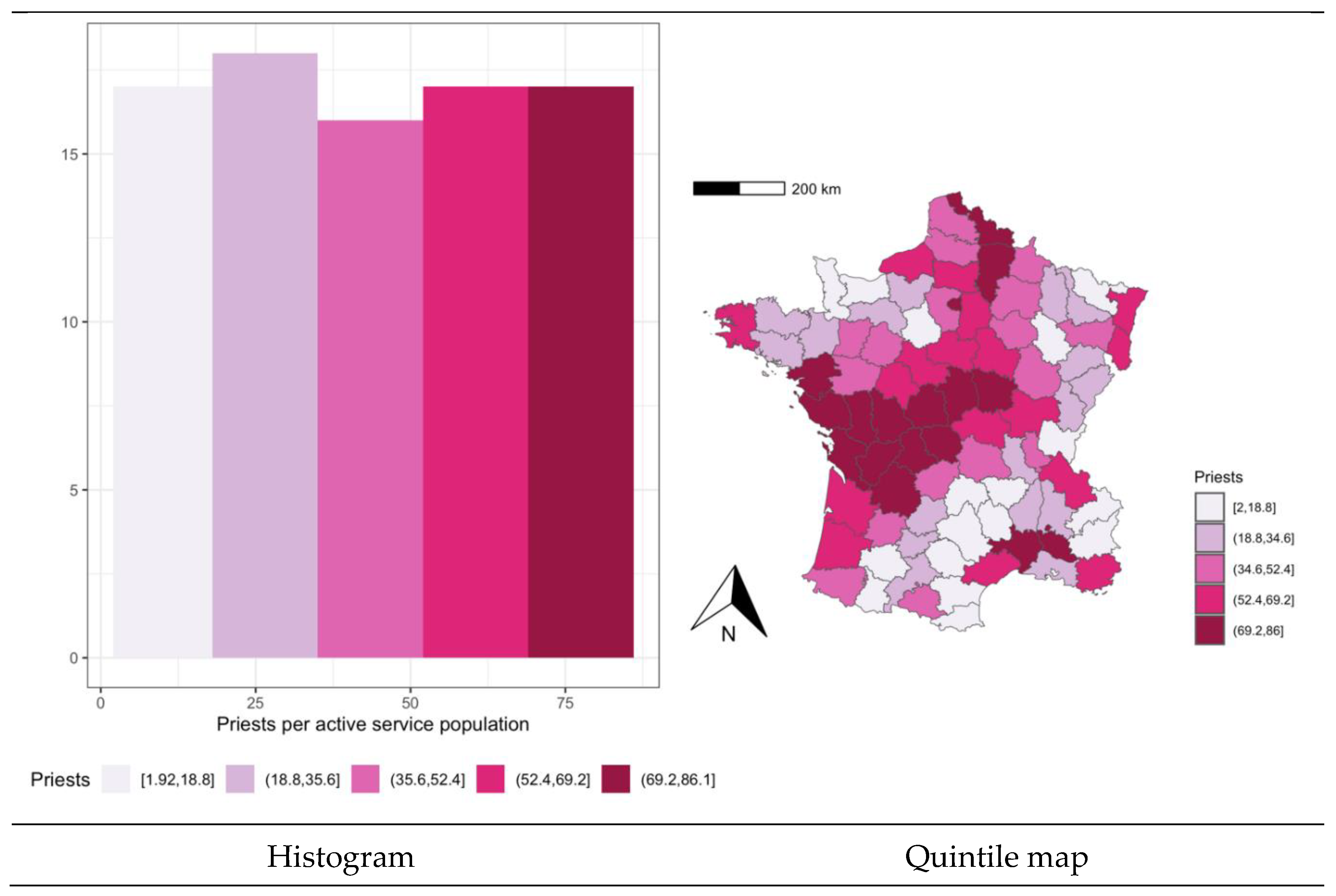
Figure 1 shows the histogram and the quintile map of the variable “clergy” representing the rate of Catholic priests per active service population in the provinces of France.
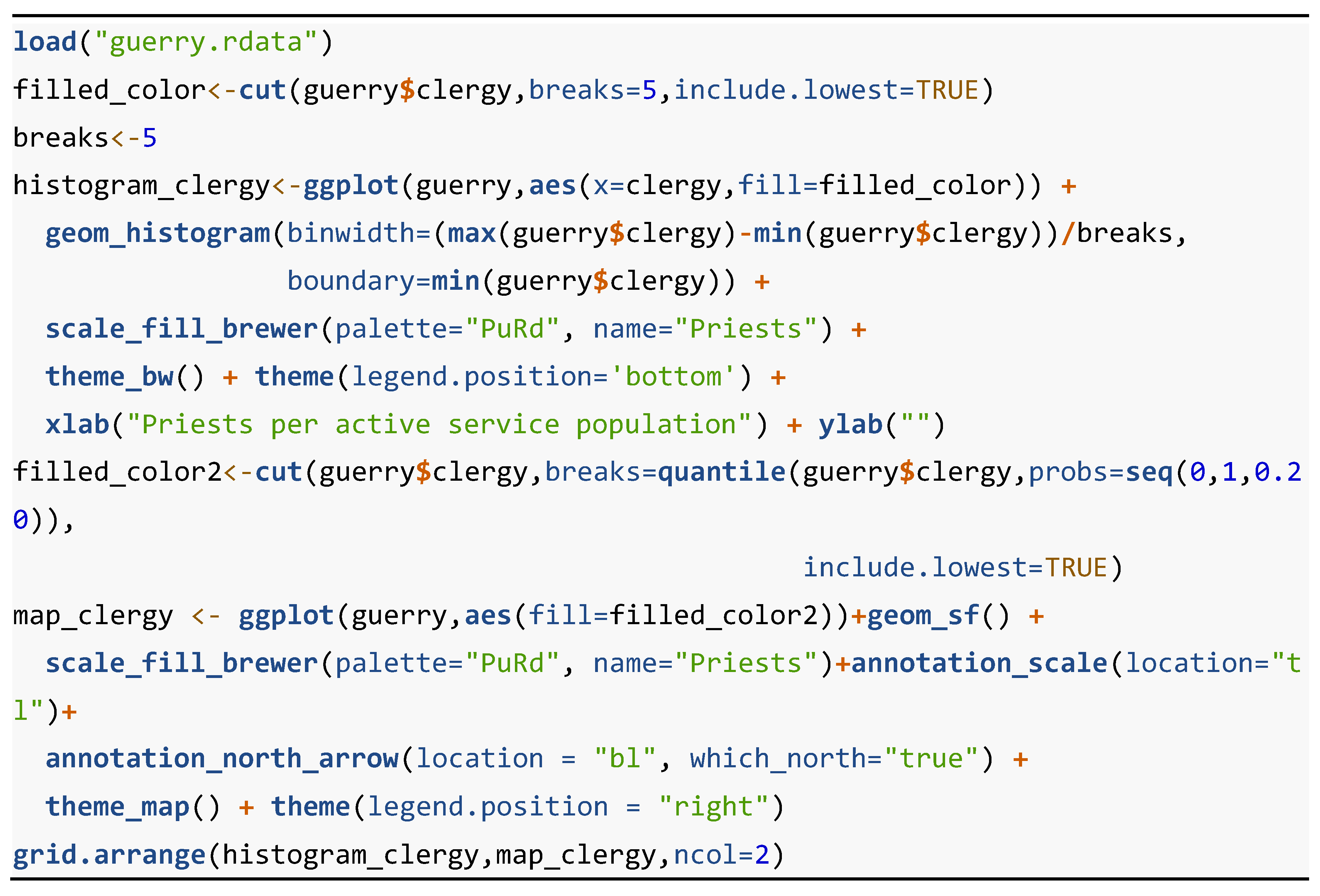
Table 1. R Code: ESDA of the rate of Catholic priests per active service population (Figure 2).
Preprints 84347 t001
The histogram creates intervals of the variable with equal length (in this case, 5 intervals of size 16.8% with approximately 17 observations each), starting from the minimum value of the variable (2%). It shows a practically uniform distribution of this variable. The quintile map groups the data into 5 categories with the same number of observations (17 in all cases), almost identically to the histogram. However, the observation of the map allows detecting that spatial units with similar values are clustered in space, uncovering the existence of positive spatial autocorrelation.
Table 1 presents the R code needed to generate the results of this figure. The following five libraries2 are required to run this code: "ggplot2", "ggspatial", "ape", "ggthemes", and "gridExtra". The main functions involved in this R code are "load", "cut", "ggplot", "geom_histogram", "annotation_scale", "annotation_north_arrow" and "grid.arrange". load{base} reload saved datasets (in this case, "guerry.rdata"). cut {base} divides the range of a numeric variable into intervals (factor variable) coding its values according to which interval they fall. ggplot is a function of “ggplot2”, which is a popular data visualization package in R programming. It stands for “Grammar of Graphics plot” and provides a consistent and structured way to create visualizations. geom_histogram {ggplot2} visualises the distribution of a single continuous variable by dividing the X axis into bins, counting the number of observations in each bin, and displaying the counts with bars. annotation_scale {ggspatial} allows creating the scale bar, which is a graphical means of depicting distance on a map. annotation_north_arrow {ggspatial} allows creating the north arrow on a map, which is a graphical representation that points to the geographical north (the option “true” points specifically to the North Pole). grid.arrange {gridExtra} allows arranging multiple graphical objects (“grobs”) on a page.
Figure 1. ESDA of the rate of Catholic priests per active service population in France’s provinces.
Preprints 84347 g001
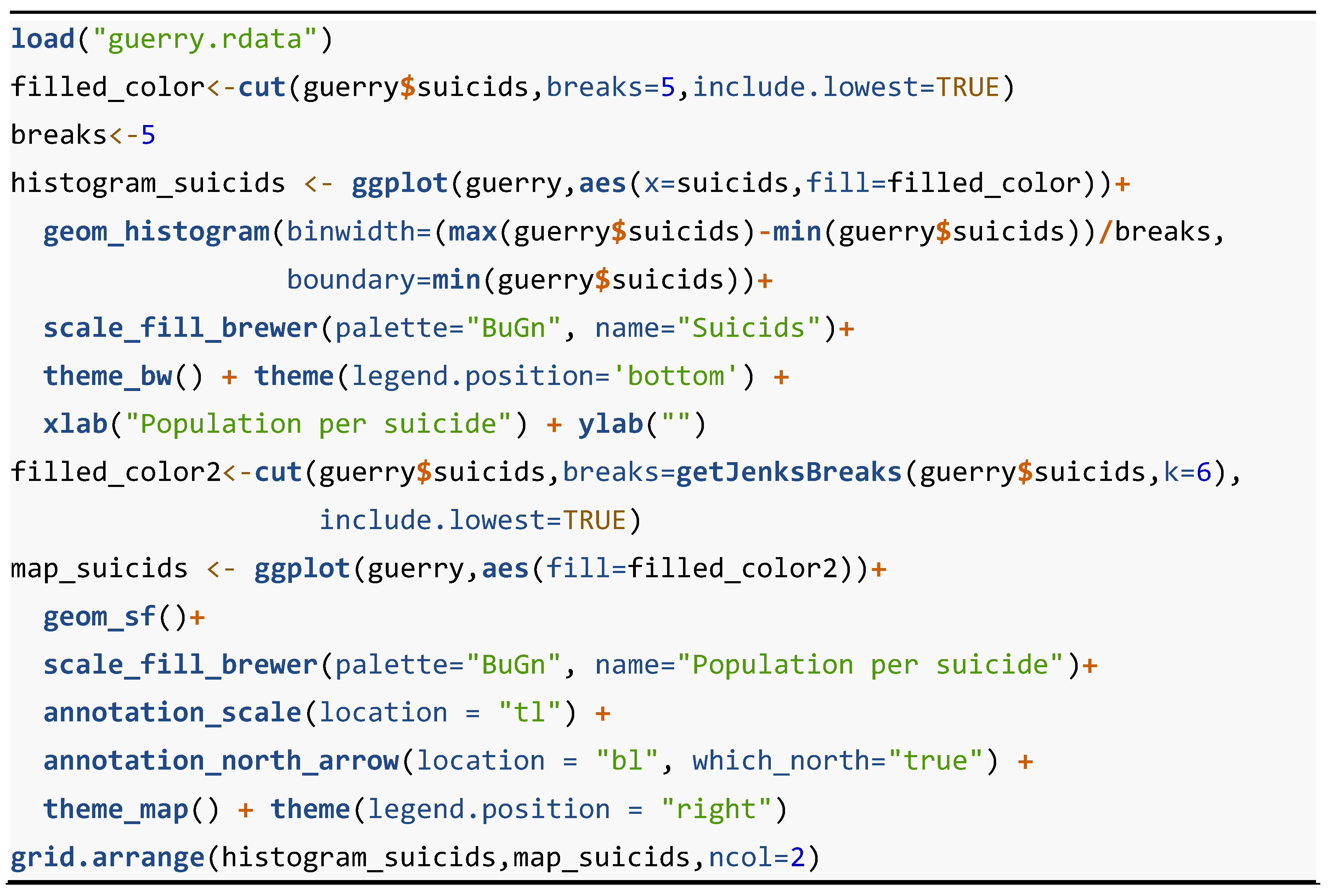
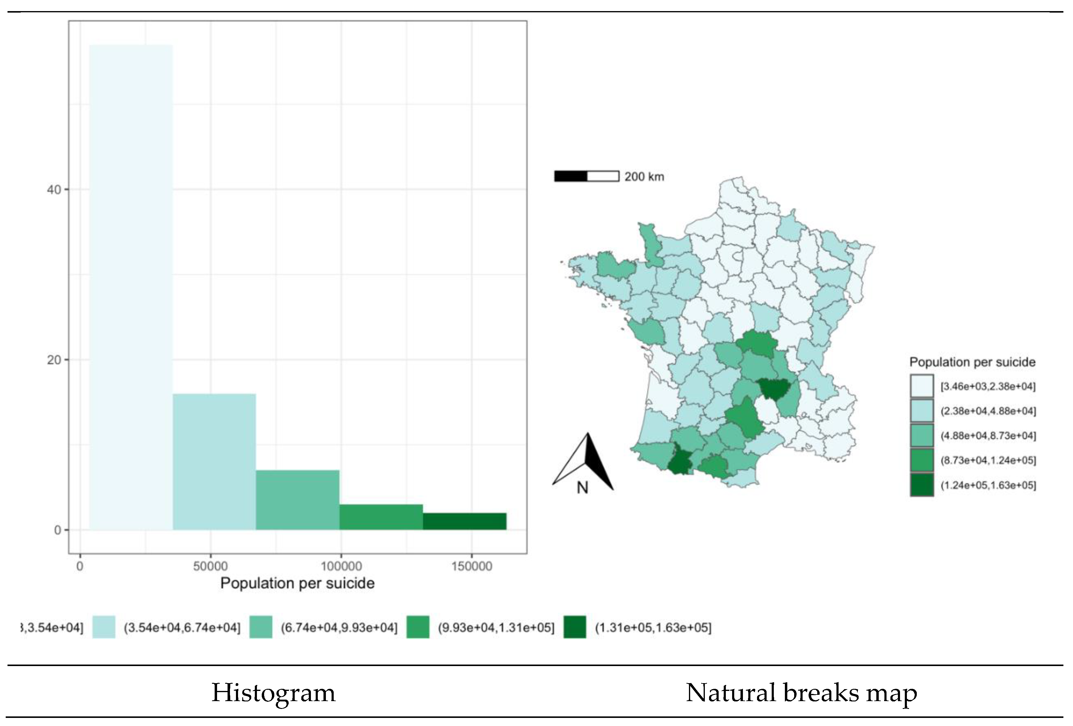
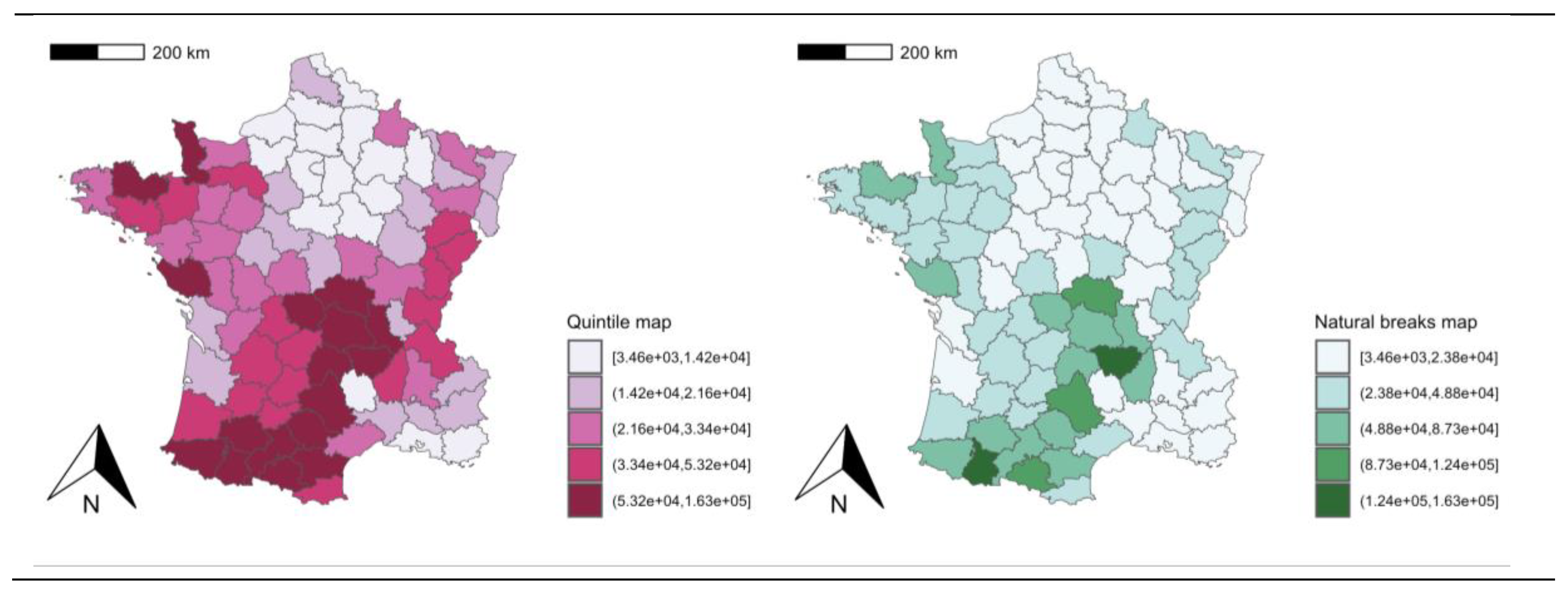
However, quintile maps are not useful when a determined variable has a non-normal distribution, as is the case for the variable “suicids” presenting the population per suicide in the provinces of France. Thus, when a variable is highly skewed or asymmetric, there is usually a high proportion of very similar values in the centre or at one extreme of the distribution, with one or more values far away from the rest at the other extreme, as shown in the histogram in Figure 2. This prevents quintiles from being defined correctly by grouping very similar values into different intervals or very different values into a single interval. In these cases, it is better to use the choropleth map of natural breaks which is the one chosen to represent the variable “suicids” in Figure 2.
The R code is shown in Table 2.
Table 2. R Code: ESDA of the rate of suicides (Figure 2).
Preprints 84347 t002
Figure 2. ESDA of the population per suicide in the French provinces.
Preprints 84347 g002
The libraries and functions required for this code are the same as above. In addition, the function and corresponding library getJenksBreaks {BAMMtools} is added, which calculates the optimum breakpoints using Jenks natural breaks optimization. The values in a variable are binned into k+1 categories (5+1 in our case), according to the Jenks’ classification method. This method is borrowed from the field of cartography, and seeks to minimize the variance within categories, while maximizing the variance between categories.
If a highly asymmetric distribution such as the suicide variable in the French provinces were represented by a quantile map, we could draw the wrong conclusions. In the quintile map in Figure 3, for example, the suicide variable obtains the highest values in the southern half and extreme west and east of France, leaving only a few northern provinces freer of this problem. However, a more appropriate representation of this variable with a map of natural breaks concentrates this phenomenon in certain provinces in the centre-south of the country.
For this reason, it is important to carry out a preliminary exploratory analysis of the variables to analyse, even to know what type of map to use, because, as Monmonier [7] rightly explains, consciously or unconsciously, it is very easy “to lie with maps".

2.2. Spatial Autocorrelation Effect: The Spatial Weights Matrix

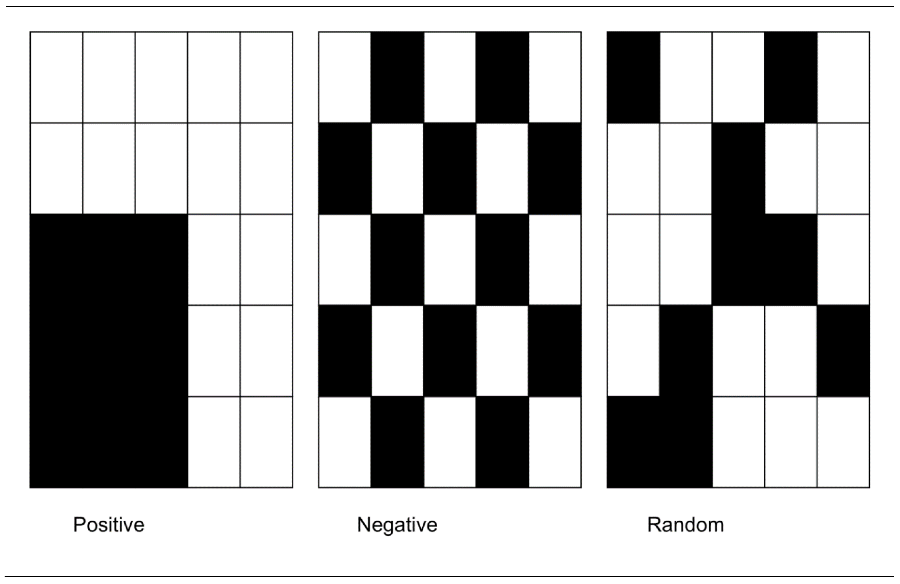
One of the most studied spatial effects so far is that of spatial autocorrelation, which is the one we will focus on in this section.3 Spatial dependence4 is said to exist in a variable when the value it takes in one observation i is influenced by the value it takes in another observation j, and vice versa (see [8]). The spatial autocorrelation effect can be positive, when spatial units with similar values tend to be together (high values close to high and low values close to low) or negative, when spatial units tend to be surrounded by neighbouring units with opposite values (high surrounded by low, and the other way around). The absence of spatial autocorrelation is known as spatial randomness. In Figure 4, various spatial patterns are shown for spatial autocorrelation and spatial randomness.
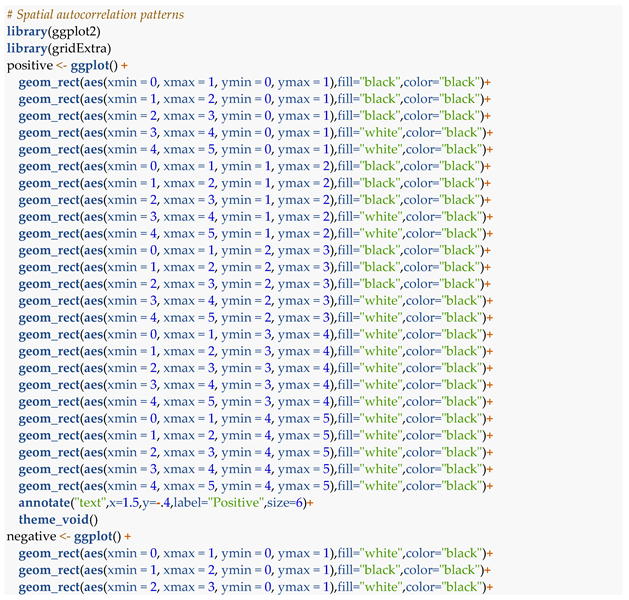
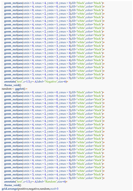
The code and R packages needed to produce this figure can be found in Appendix A.1. The following five libraries are required to run this code: "ggplot2" and "gridExtra". The main functions involved in this R code are " geom_rect" and " grid.arrange". geom_rect {ggplot2} is a geometric object (“geom”) that draws a rectangle using the locations of the four corners (“xmin”, “xmax”, “ymin” and “ymax”). grid.arrange {gridExtra} is defined as above.
The concept of autocorrelation alone refers to the modelling of a variable with itself. Thus, when referring to serial autocorrelation in econometric models, we state to the fact that the past values of a variable affect the present values of the same variable. y t = f y t 1 , , y 1 . In this case, it is a one-way interaction of the variable: from the past to the present. However, the influence of geographical space is not unidirectional but multidirectional, in the environment or neighbourhood of a unit of analysis. It is therefore crucial to define the concept of spatial neighbourhood, in order to carry out any spatial analysis.
The spatial neighbourhood matrix, W n × n , also called spatial weights matrix, shows the relationship among n spatial units under analysis. This matrix defines the spatial neighbourhood condition and thus the interaction between the spatial units. In its simplest form, the spatial weights matrix is a symmetric and binary matrix, where the element w i j = 1 if spatial units i and j are neighbours and zero if they are not. By convention, it is established that w i i = 0 , i.e., a spatial unit cannot be a neighbour of itself. There are different criteria for defining this matrix depending on the process to be modelled and the characteristics of the data. But basically, we could identify the following two groups of spatial weighting matrices: spatial contiguity matrices and spatial weights matrices based on distances.

2.2.1. Spatial Contiguity Matrices

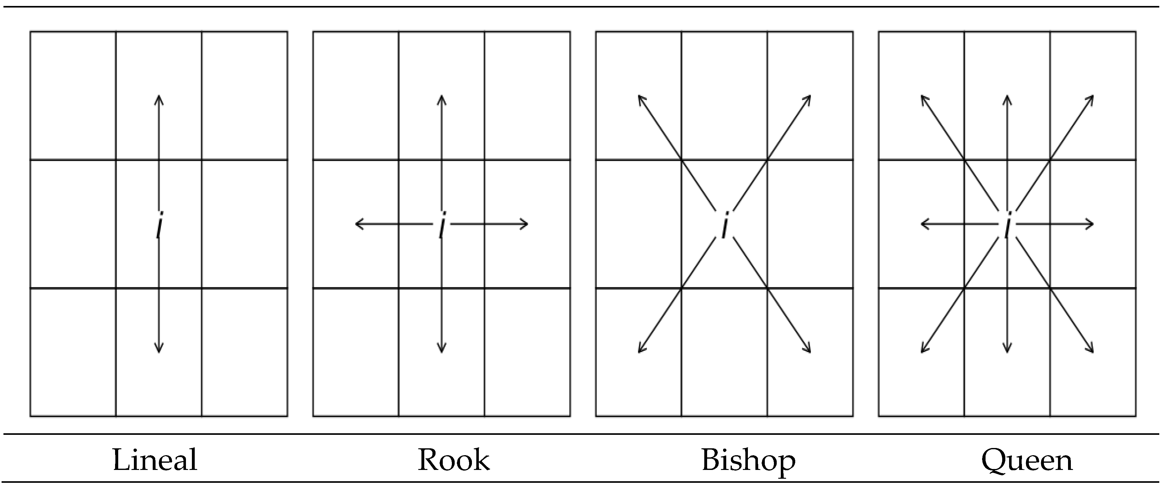
When working with a map in which the geographical units are polygons, one of the criteria presented in Figure 5 can be used to define the W matrix.
The linear criterion is the simplest. It considers as neighbours to a given spatial unit i all those units located to the north and south of this unit, provided they share a border in common with i. This criterion could also be applied if the neighbouring and contiguous units to i were located to the east and west sides.
The rest of the contiguity criteria follow the moves on a checkerboard to define spatial unit i’s neighbourhood. The construction of a neighbourhood matrix under the rook criterion implies considering as neighbours of spatial unit i those spatial units located in the four cardinal points (north, south, east, and west), provided that they share a common border with this unit. The use of the bishop criterion considers as neighbours of unit i those units located in the secondary or lateral cardinal points (north-east, north-west, south-east or south-west) of spatial unit i, provided that they have at least one point in common.
The queen criterion is the most complete of all by considering as neighbourhood of spatial unit i those spatial units located in all main and secondary cardinal directions, provided that they have a point or a border in common with spatial unit i (Martori et al. [9]). Since the neighbourhood criterion in all these W matrices is based on the units or regions having a common border (edge or point), they are also called spatial contiguity matrices.
In certain contexts, such as spatial regression models, spatial weight matrices are row standardised, so that their elements are transformed as follows:
w i j * = w i j J = 1 n w i j
In simple words, each element of a row of the matrix W* is divided by the sum of the values of that row. This ensures that each element of the standardised spatial weights matrix lies between the values 0 and 1, and that the sum of the values in each row is always equals to 1.
The R code required for the construction of spatial contiguity matrices is presented in Table 3.
The "spdep" library is required to run this code (see Bivand and Wong [10]). It is a collection of functions to create spatial weights matrix objects from polygon 'contiguities', point patterns by distance and tessellations. It also loads the "spData" package (a group of spatial datasets for demonstrating, benchmarking, and teaching), which is underpinned by some legacy packages ("maptools", "rgdal" and "rgeos"). They will be retired during 2023, joint to all the "sp" classes, methods, and functions, and "sf", ”terra" or other packages will be needed instead.
The main functions involved in this R code, besides “load", are “poly2nb", “nb2listw" and “plot". poly2nb {spdep} builds a neighbours list based on regions with contiguous boundaries, that are sharing one or more boundary points. nb2listw {spdep} adds a weights list with values given by a coding scheme style, the most commonly used being B (basic 0-1 binary coding) and W (row standardised).
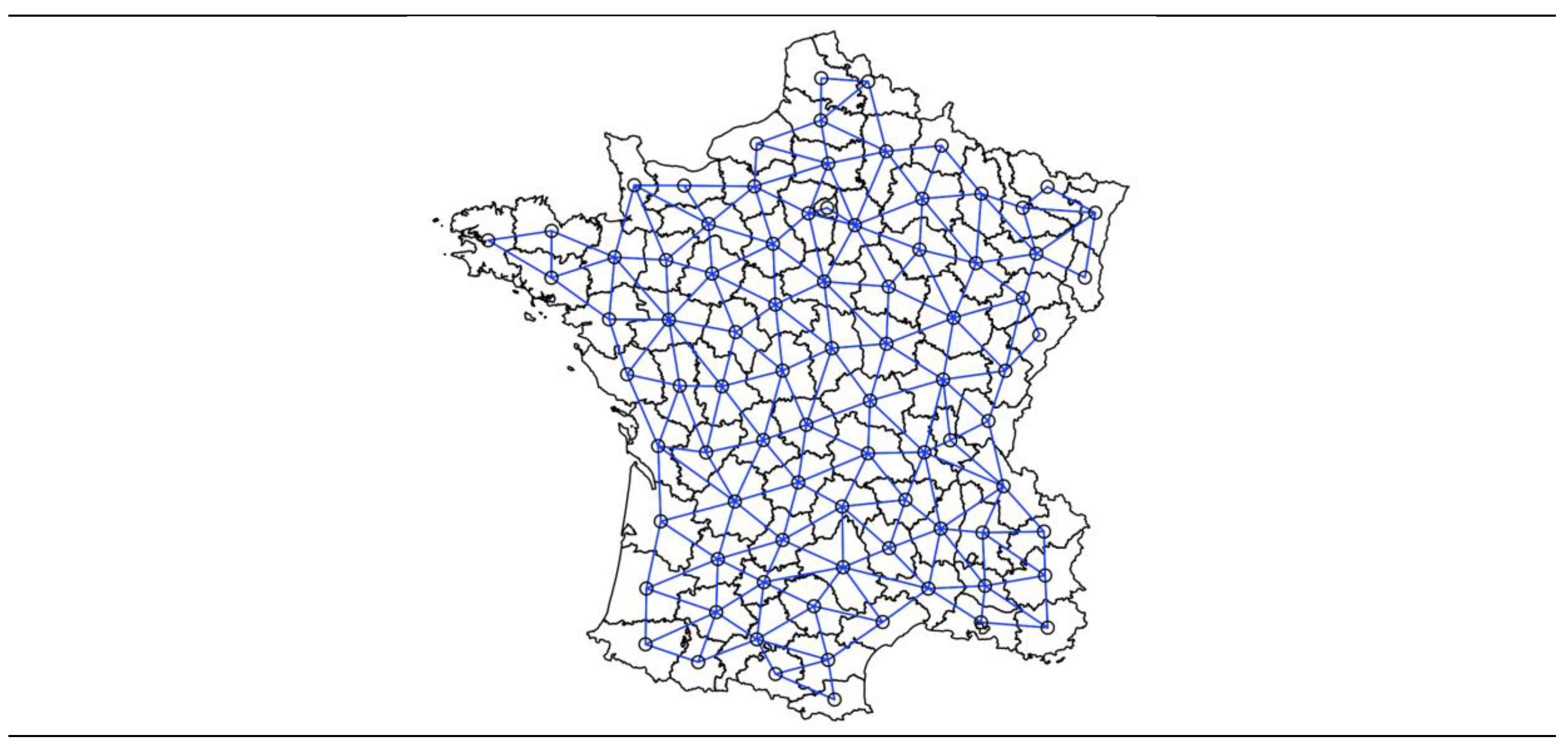
plot is more than a function, it is placeholder for a family of related functions which allows to create a plot passing two vectors (of the same length), a dataframe, matrix, map, or even other objects, depending on its class or the input type. This function makes it possible to represent the spatial neighbourhood network of the W matrix corresponding to the provinces of France (Figure 6).
Figure 6. Neighbourhood network of a queen spatial contiguity matrix.
Preprints 84347 g006
The construction of a rook-style spatial contiguity matrix requires the same packages and functions, but the ”queen” parameter of the “poly2nb" function must be changed to "FALSE ", as in Table 4. When working with administrative regions, differences in the spatial network of the queen- and rook-based contiguity matrices are almost non-existent, as practically all regions have more than one point in common.

2.2.2. Spatial Weights Matrices Based on Distances

There are situations where spatial contiguity matrices are not the most appropriate. For example, when spatial data are isolated points or locations, with no possibility of having common boundaries or in the case of polygonal data with "islands", i.e., units with no neighbours because they do not have a common boundary with other units in the system. The zero-neighbour situation should be avoided in spatial weight matrices as it affects the calculations of the spatial autocorrelation statistics in which they participate.
In these cases, it is more convenient to define neighbourhood matrices based on distance-based criteria. These W matrices can be specified in two ways: local and global.
a)
Local which, for each spatial unit, consider as a discrete or local neighbourhood domain, such as a given number of k nearest neighbours or a distance radius. As for the k nearest neighbour W matrix, its formal definition is the following:
w i j = 1                 ;             d i j d i k w i j = 0               ;             d i j > d i k   ;   i
where dij is the distance between i and j and d i k is the distance at which each spatial unit i reaches a predetermined number of k nearest neighbours. Hence, in this type of configuration, all spatial units have exactly the same number k of spatial neighbours.
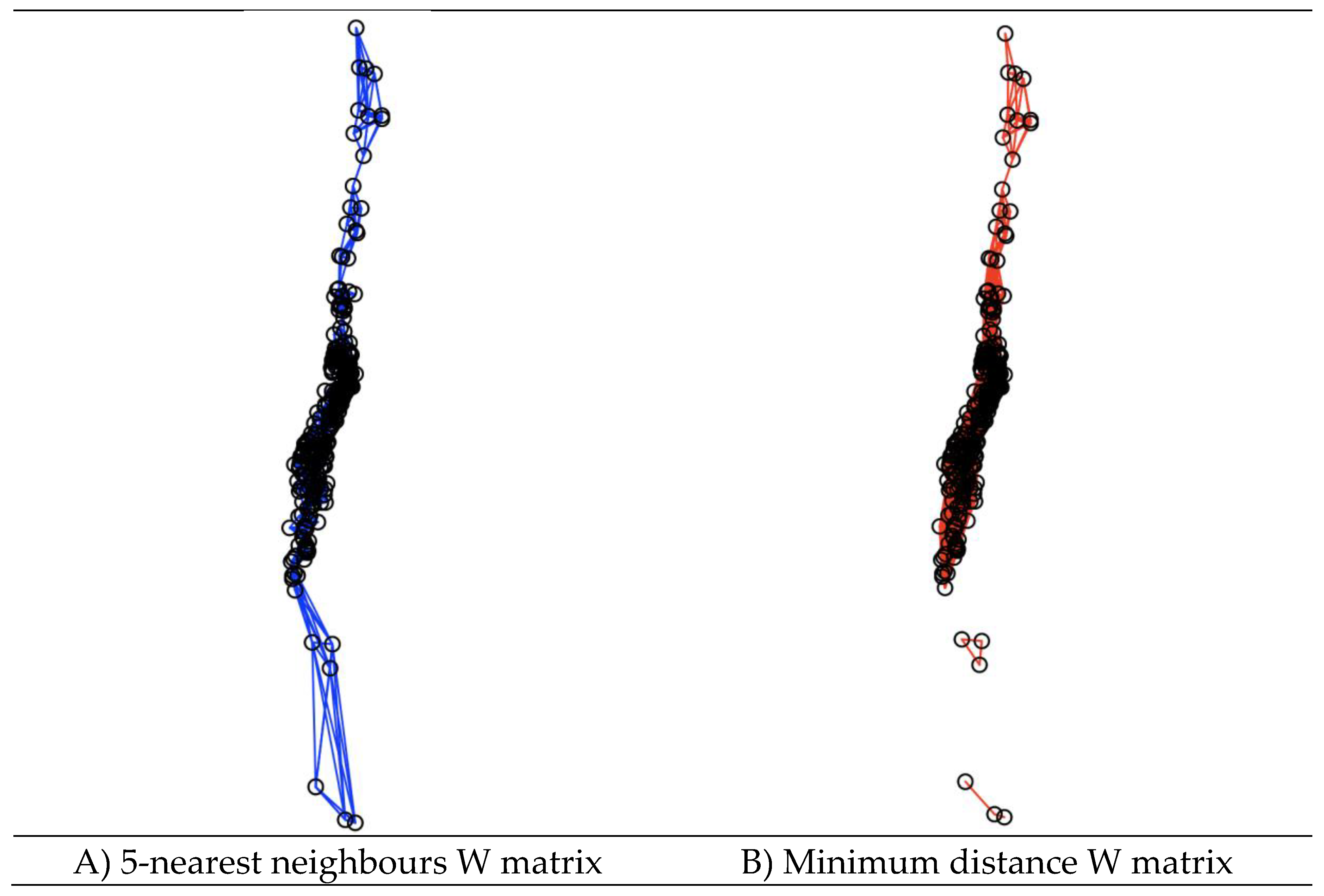
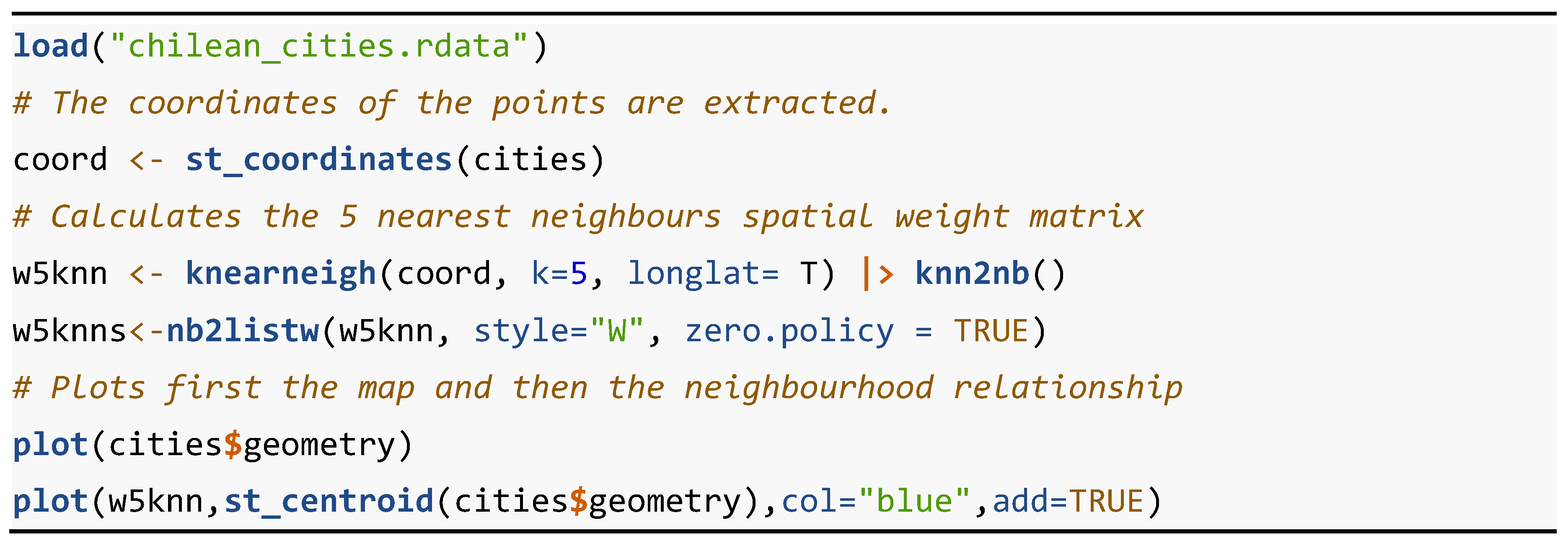
To illustrate the definition of the W matrices based on distances, a point map containing the centroids of the main Chilean cities, used in Vallone and Chasco [11] will be used. The R code required for the construction of k-nearest neighbour matrices is presented in Table 5. Two libraries are required to run this code: "spdep", which is defined as above, and "sf" (see Pebesma et al. [12]). The main functions involved in this R code, in addition to those already presented, are “st_coordinates", “knearneigh ", “knn2nb”, “nb2listw”, “plot" and “st_centroid". st_coordinates {sf} retrieve the coordinates of spatial objects of class sf, sfc or sfg, in a matrix form of n rows and two columns for X and Y. knearneigh {spdep} returns a knn object, which is a matrix with the indices of points belonging to the set of the k nearest neighbours of each other; if longlat=TRUE, great-circle distances are used.5 knn2nb {spdep} converts a knn object returned by the knearneigh function into a neighbours list of class nb with a list of integer vectors containing the index number (ID) of the neighbour regions. st_centroid {sf} is a geometric operation on a simple feature geometry (sf, sfc and sfg spatial objects), returning its centroid, which will be an object of the same class.
Figure 7A presents the neighbourhood network corresponding to the W matrix of 5 nearest neighbours of the cities in Chile. As can be seen in the south of Chile, the neighbourhood network seems somewhat unrealistic as it connects cities that are actually more than 1,400 kilometres away by road from each other, as is the case of Puerto Aysén (Region XI) and Punta Arenas (Region XII).
Another local specification of the spatial weight matrices is based on the determination of a neighbourhood distance radius around each geographical unit. For example, the minimum distance W matrix considers as radius the minimum distance necessary for all regions or locations to have at least one neighbour. It is specified as follows:
w i j = 1               ;             d i j < d m i n w i j = 0               ;             d i j > d m i n
for d m i n the minimum distance necessary for all geographical units to have at least one neighbour.
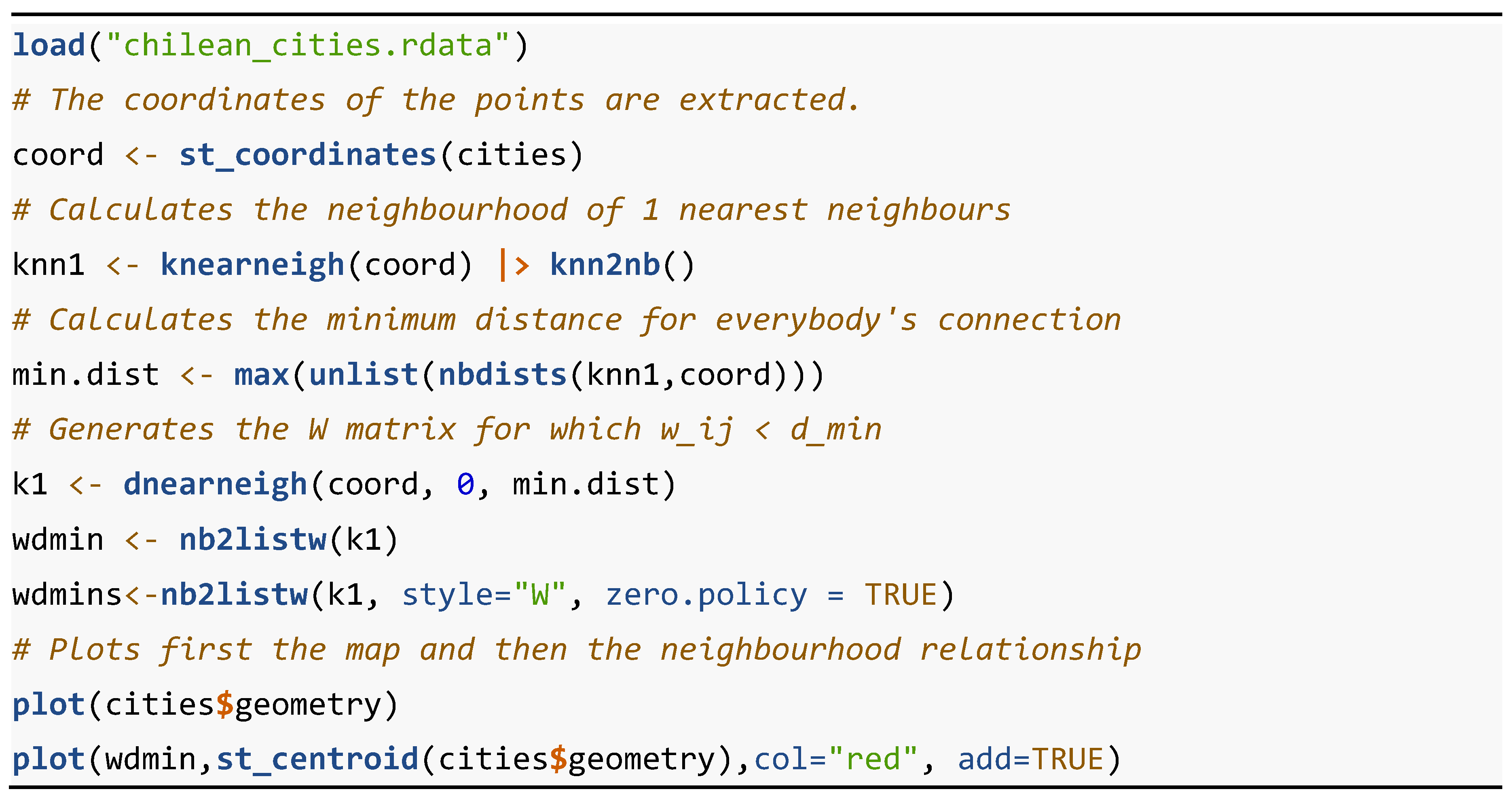
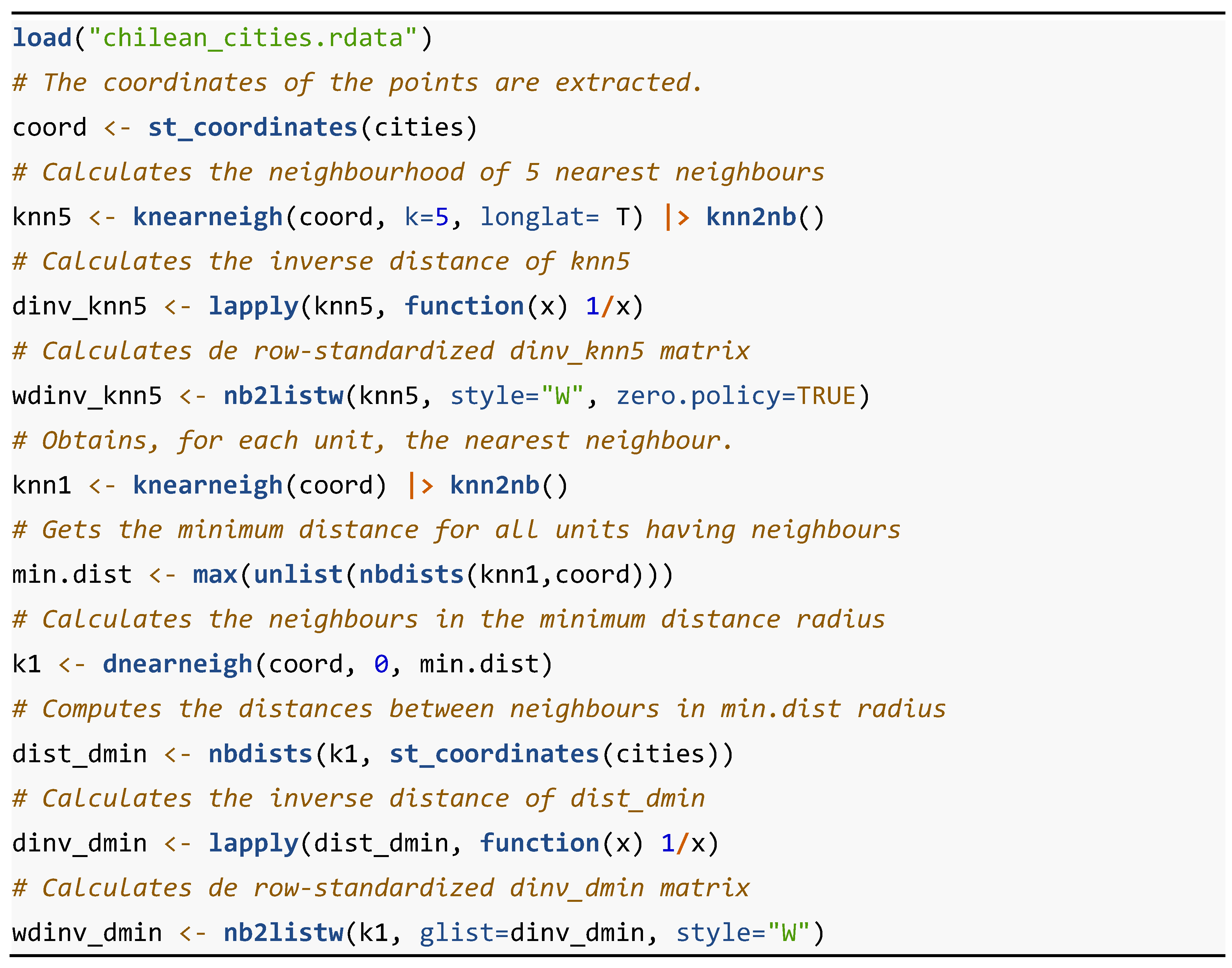
The R code required for the construction of minimum distance neighbour matrices is presented in Table 6.
Table 6. R Code: construction of the minimum distance W matrix (Figure 7B).
Preprints 84347 t006
Figure 7. Neighbourhood network of distance-based W matrices for the Chilean cities.
Preprints 84347 g007
The libraries and functions needed to calculate these matrices are the same as in the previous cases, except for the functions “max” and “unlist” which are part of the basic R functions. and “nbdists”. max {base} returns the maximum of all the values present in its argument. unlist {base} simplifies a list structure to produce a vector which contains all the atomic components (logical, integer, real, complex, character and/or raw). nbdists {spdep} returns the Euclidean distances along the spatial neighbour links of an object type nb.
Figure 7B presents the neighbourhood network corresponding to the W matrix of minimum distance of the cities in Chile, which according to the integer atomic argument “min.dist” is equal to 215 km. Therefore, the cities of Puerto Aysén and Punta Arenas no longer appear to be linked in the neighbourhood network. Both cities are connected to other neighbouring cities in their respective regions, each forming its own urban network.
a)
Global specifications of the spatial weight matrix consider as neighbours of each of the geographical units the rest of the units of the system, on a continuous basis, although with different weights or values depending on the distance that separates them. For example, the inverse distance spatial weight matrix, whose elements are defined as a gravity function is defined as follows:
w i j = d i j α
for α 0 , a friction parameter.
Although it is a matrix with non-zero elements (except for the main diagonal), from a certain distance between points the value of the w i j elements will be practically zero. For this reason, a distance radius could usually be established to simplify the calculations (e.g., in the case of spatial systems with a large number of elements or regions), considering all the units beyond this radius as non-neighbours (wij = 0 ).
Table 7 presents the R code with the process of obtaining the inverse distance spatial weights matrix.
It establishing two types of cut-offs for each spatial unit: firstly, the group of 5 nearest neighbours and secondly, the radius of the minimum distance for which all spatial units have at least one neighbour. The libraries and functions needed to calculate these matrices are the same as in the previous cases, except for the function “lapply”. lapply {base} returns a list of the same length as an “x” argument, each element of which is the result of applying a function to the corresponding element of “x”..
Finally, the application of the spatial weights matrix to calculate a spatially lagged variable or spatial lag is presented. The spatial lag variable Wy of the variable y is obtained by premultiplying the matrix W by that variable, as presented in the following example.
y = 120 300 240 60 180     ;     W y = 0 1 / 4 0 1 / 2 1 / 3         1 / 3 0 1 / 2 1 / 2 1 / 3         0 1 / 4 0 0 1 / 3         1 / 3 1 / 4 0 0 0         1 / 3 1 / 4 1 / 2 0 0 120 300 240 60 180 = 540 / 3 600 / 4 480 / 2 420 / 2 660 / 3 = 180 150 240 210 220
According to the matrix W, the first spatial unit has three neighbours: units 2, 4 and 5. Therefore, each element of the first row of the standardised matrix, W*, is 1 / 3 . The first element of the spatial lag variable is equal to 180, which is the average value of the variable y ’s neighbours of the first spatial unit: ( y 2 + y 4 + y 5 3 = 300 + 60 + 180 3 = 540 3 = 180 = W * y 1 . Therefore, each element i of the spatial lag variable, W * y i , is a weighted average of the values of the variable y in the units neighbouring the spatial unit i .

2.3. Spatial Autocorrelation Measures

2.3.1. Moran’s Scatterplot

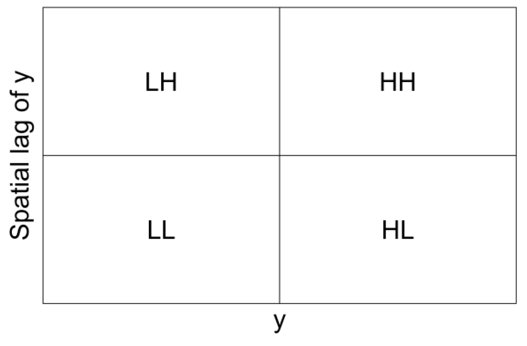
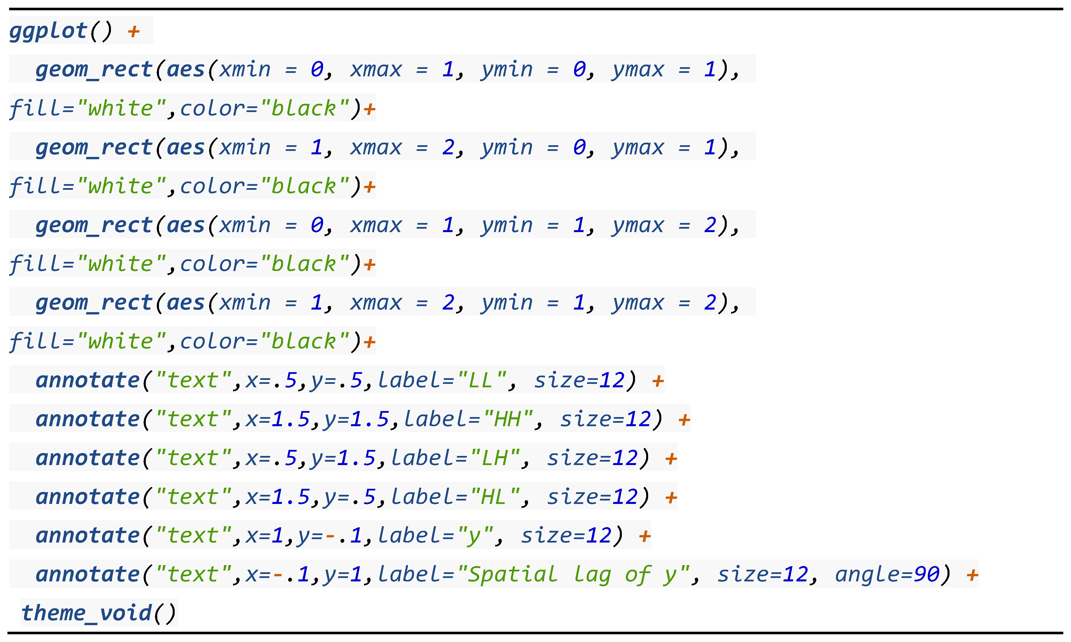
A good tool for understanding spatial autocorrelation statistics is the Moran’s scatterplot (see Anselin et al. [13]), which relates a variable to what is happening in its environment through its spatial lag in a scatter plot. Figure 8 shows this diagram: on the horizontal axis are the values of a variable and, on the vertical axis, the values of its respective spatial lag. Therefore, the origin of coordinates corresponds to the mean value of both variables. This diagram allows the identification of four quadrants: the first quadrant, called "High-High" (HH) contains the spatial units with values of both variables higher than the mean value of the system. The spatial units located in the third quadrant, "Low-Low" (LL) are the values of the variables below the average. Values located in the second and fourth quadrants, "Low-High" (LH) and "High-Low" (HL), respectively, are those where the main variable is below/above the mean, with the values of their corresponding spatial lag being above/below the mean, respectively.
The R code with the process of obtaining a Moran’s scatterplot representation is presented in Table 8. The only library needed to represent this diagram is "ggplot2". The functions employed, not previously presented, are “annotate” and “theme_void”. annotate {ggplot2} adds geometric objects (“geoms”) to a plot when their properties are introduced as vectors, which is useful for adding text labels (as it is the case here). theme_void {ggplot2} a completely empty theme of the non-data display.
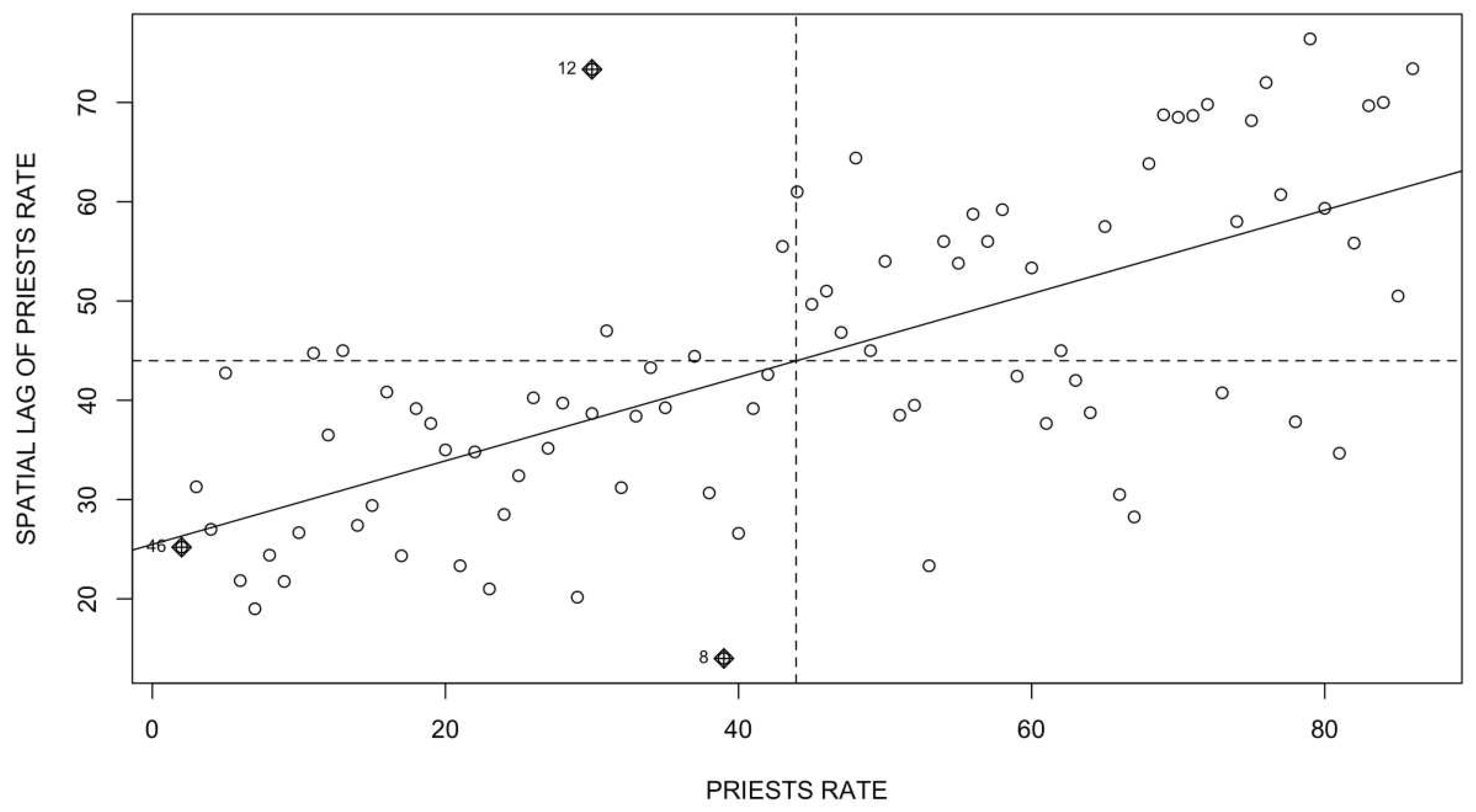
If the values of the scatterplot are mostly located in the "HH" and "LL" quadrants, it means that spatial units with high/low values of the variable (above/below the average) are surrounded by spatial units that, on average, also have high/low values of the variable, respectively. This is an indication of the existence of positive spatial autocorrelation. If the concentration is in the "LH" and "HL" quadrants, it would be indicative of negative spatial autocorrelation: low surrounded by high and high surrounded by low, respectively. Using the same distribution rate of Catholic priests used in section 2.1 and using a spatial weights matrix defined with the queen criterion, Figure 9 presents the corresponding Moran scatterplot.
The R code with the process of obtaining this Moran’s. scatterplot is presented in Table 9. The only library needed to represent this diagram is "spdep". A new function is employed, “moran.plot”. moran.plot {spdep} plots a spatial variable data against its spatially lagged values.
Figure 9 shows evidence of positive autocorrelation, i.e., French provinces with high/low rates of Catholic priests tend to be surrounded by provinces that, on average, also have high/low rates of Catholic priests, respectively. The Moran’s scatterplot is only a graphical tool that needs to be complemented by more precise statistical measures, such as the Moran's I index of spatial autocorrelation.
Figure 9. Moran’s scatterplot of the rate of Catholic priests in the French provinces.
Preprints 84347 g009

2.3.2. Global Moran’s I Statistic

The Moran’s I statistic of spatial autocorrelation is calculated as:
I = n S 0 i = 1 n j = 1 n w i j z i z j i = 1 n z i 2
where n is equal to the number of spatial units in a system, S 0 = i = 1 n j = 1 n w i j is the sum of all the elements, wij, of the spatial weights matrix, z i = y i y ¯ is a variable y i expressed in deviations from the mean value ( y ¯ ), and the summation over j is such that only i ’s neighbouring values ( j J i   ; i j ) are included.
As can be seen, the second factor of Equation (6) consists of a quotient of the covariance of the variable y with its corresponding spatial lag, Wy, in the numerator and, in the denominator, the variance of the variable y or the product of the standard deviations of both variables (since both values are equal). As for the first factor of Equation (6), it is equal to unity when the spatial weight matrix is row-standardised, since, in these cases, the sum of the weights is always equal to the sample size n. Hence, the Moran’s I index can be interpreted as a linear correlation coefficient between a variable and its spatial lag, whose values lie within the range 1 , 1 , so that the sign of the indicator coincides with the type of spatial autocorrelation: positive values ( I > 0 ) are indicative of positive spatial autocorrelation and negative values ( I < 0 ) are indicative of the existence of negative autocorrelation. Unlike what happens with the classical linear correlation coefficient, the complete absence of spatial autocorrelation does not correspond to the value zero exactly, except when n tends to infinity, but to the expression 1 / n 1 .
Moran’s I value is usually represented in the Moran scatterplot with the linear regression line. For example, in Figure 9, the regression line of the variable y on Wy is plotted, which in this case has a positive slope. The higher the degree of spatial autocorrelation in the variable y, the steeper the slope of the regression line. In addition, it is possible to calculate the level of statistical significance of the Moran’s I value, through a randomisation process, by considering the null hypothesis of no spatial autocorrelation and having as alternative the hypothesis of spatial autocorrelation, both positive and negative ([8]).
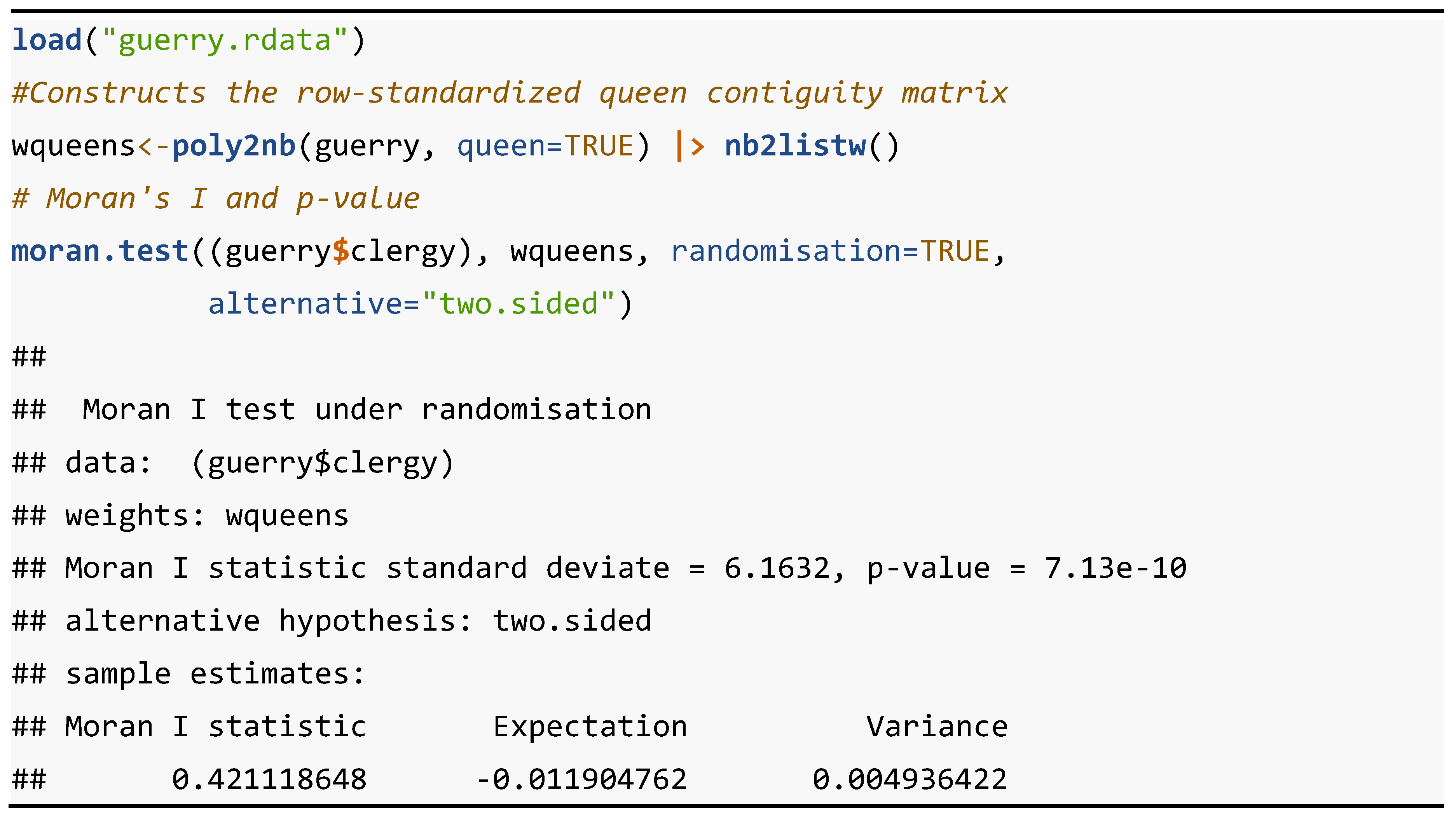
The R code with computation of the Moran’s I indicator of the variable rate of Catholic priests plotted in Figure 9 is presented in Table 10. The only library needed to represent this diagram is "spdep". A new function is employed, “moran.test”. moran.test {spdep} calculates the Moran's I test for spatial autocorrelation of a variable using a spatial weights matrix in weights list form.
The p-value of 7.12 · 10 10 does not allow to accept the null hypothesis of spatial randomness, so given that the value of I = 0.421 is of positive sign, we can conclude that the variable rate of Catholic priests has positive spatial autocorrelation in its provincial distribution in France.
As indicated in [5], there are variables whose distribution does not allow the null hypothesis of no spatial autocorrelation to be rejected. In these cases, it must be checked whether the absence of spatial autocorrelation occur globally, across the entire surface of the spatial system, or whether, on the contrary, there are certain spatial clusters of similar or dissimilar values locally, in some areas of the system. In other words, the spatial autocorrelation effect can occur globally and locally.

2.3.3. Local Moran’s I Statistics

The effect of local spatial autocorrelation can be measured from LISA (Local Indicators of Spatial Autocorrelation) statistics and maps. LISA statistics are calculated as a decomposition of global spatial autocorrelation statistics, such as Moran's I test. In this way, it is possible to know the individual contribution of each spatial unit, and its environment, to the formation of the value of the global statistic. Moreover, it is possible to obtain, for each individual value and its neighbourhood, the level of statistical significance following a randomisation approach, as in the previous case (see Chasco [14]).
The formal expression of the local Moran’s I statistics is the following:
I i = z i j = 1 n z j 2 j = 1 n w i j z j
where the values of the variable z i are expressed in deviations from the mean, an j only comprehends i ’s neighbours. For ease of interpretation, the weights w i j may be row-standardized, and by convention, w ij = 0 .
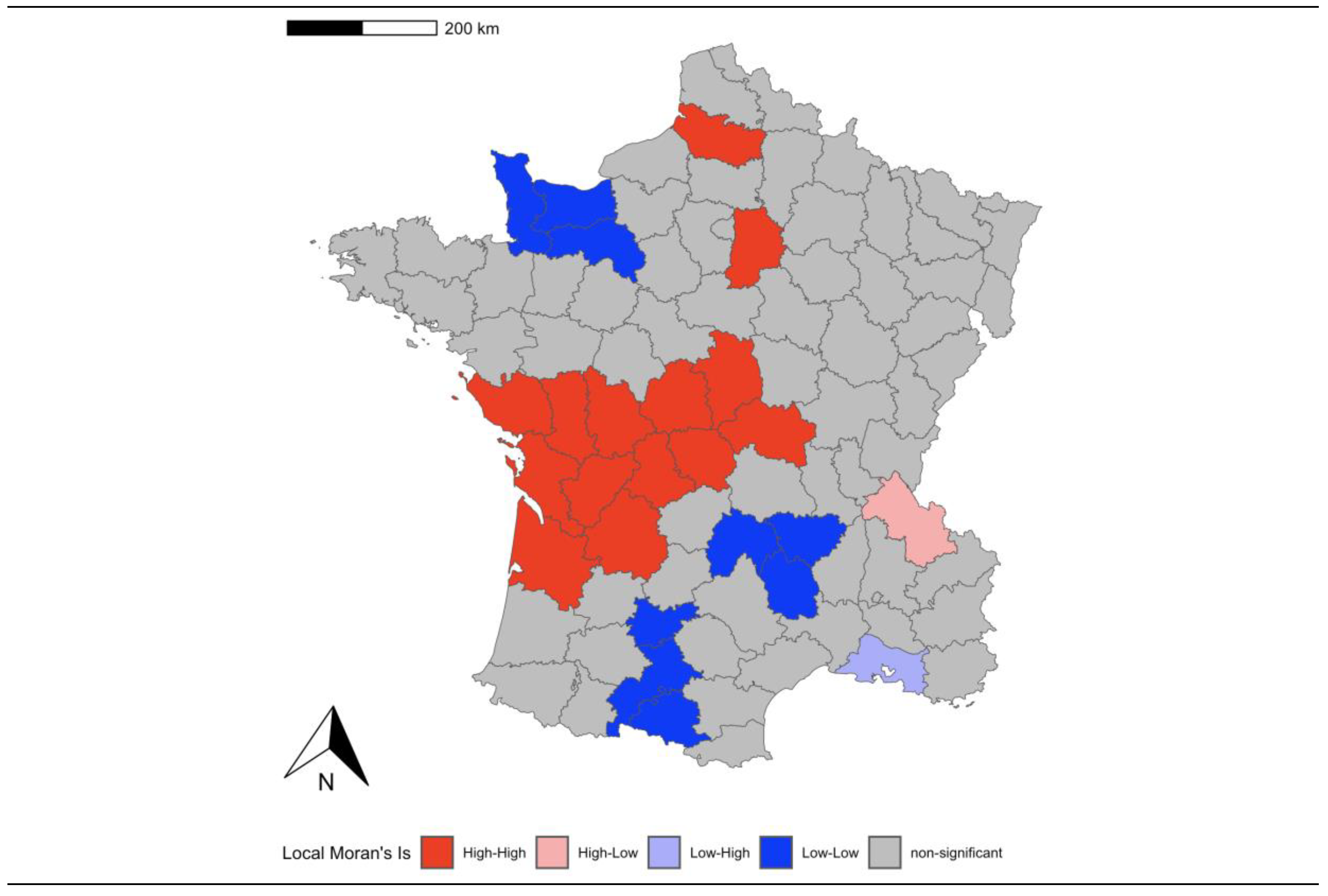
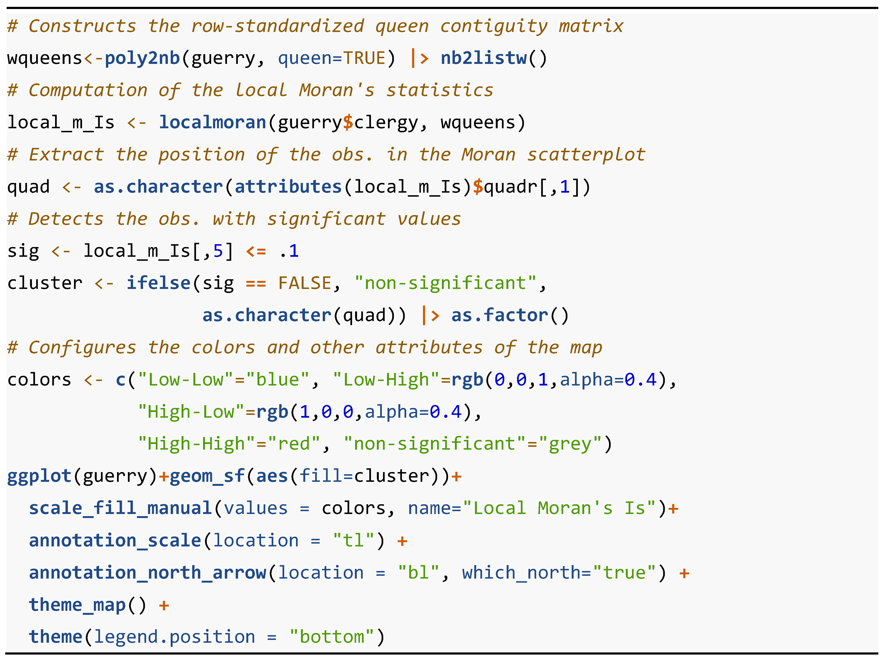
As demonstrated in Anselin [15], a test for significant local spatial autocorrelation may be calculated by taking a conditional randomization approach. In this paper, it is also derived that the global I indicator can be expressed as an average of the local I i statistics, corrected by a proportionality factor. Hence, it is possible to identify extreme values of I i by, e.g., identifying outliers in a box plot, which will indicate the importance of the spatial unit i in determining the global I . They are not necessarily statistically significant, but are only similar to the identification of outliers, leverage, and influence points in the Moran’s scatterplot (see Figure 9). In the map in Figure 10 we can find the hot spots (high values) painted in red and the cold spots (low values) painted in blue.
The R code with the process of obtaining the local Moran’s statistics and map is presented in Table 11. The libraries needed to represent this diagram are "spdep", "ggplot2", "ggspatial", "ggthemes" and "grDevices", which contains functions for graphics devices and support for colours and fonts. The functions employed, not previously presented, are “localmoran”, “as.character”, “attributes”, “ifelse”, “as.factor”, “c”, “rgb” and “scale_fill_manual”.
localmoran {spdep} computes the local Moran's I statistics for each spatial unit, based on a specified spatial weights object, joint to their corresponding returned “z-value” (significance level) that may be used as a diagnostic tool. as.character {base} creates a character vector of the specified length. attributes {base} returns an object's attribute list, understanding by attribute a set and not a vector, i.e., the order of the elements does not matter, but they must have unique names. ifelse {base} applies to all the elements of a vector, in a single call, two functions: if {base}, which is used to cause an operation to be executed only if a certain condition is met, and else {base}, which is used to state what to do in case a condition is not met. as.factor {base} encode a vector as a factor, being the factor levels ordered when the argument “ordered” is TRUE. c() {base} returns a vector (a one-dimensional array). rgb {grDevices} creates colours corresponding to the given intensities (between 0 and max) of the red, green, and blue primaries, the colour specification being referred to the standard sRGB colour space (IEC standard 61966). scale_fill_manual {ggplot2} define both colour and fill aesthetic mappings.
Figure 10. Moran’s scatterplot of the rate of Catholic priests in the French provinces.
Preprints 84347 g010

3. Cross-Section Spatial Econometric Models

3.1. Modelling Strategies for Spatial Autocorrelation Models

Spatial cross-sectional models are a particular case of cross-sectional econometric models and, as is the case with them, they must be identified before proceeding to their estimation and testing. Hence, it is important to follow a specific identification or modelling strategy for spatial models, which allows the researcher to know the correct population parameters from the observation of a data sample.
Traditionally, spatial econometrics has solved this problem by assuming that the model specification is a priori known, either from an existing economic theory, or from the results obtained by the application of an ESDA on the variables of the model, or by applying certain strategies consisting of the comparison of several competing models. Within the latter option, we can highlight two widely used modelling strategies: the one that goes from the specific (basic model without spatial autocorrelation effects) to a general model (with spatially lagged explanatory variables), STG, and the one that starts from a general model (the spatial Durbin model) to end up in a simpler spatial autocorrelation model or the basic regression model itself without spatial effects, GTS. But, from these two previous approaches, it is possible to propose a third hybrid strategy, which considers the good properties of the previous ones.

3.1.1. Anselin’s Specific-To-General Strategy (STG)

The STG strategy, also known as "classical", was proposed by Anselin ([8]). The starting point of this strategy is a basic linear regression model without spatial effects:
y = α ι n + X β + ε
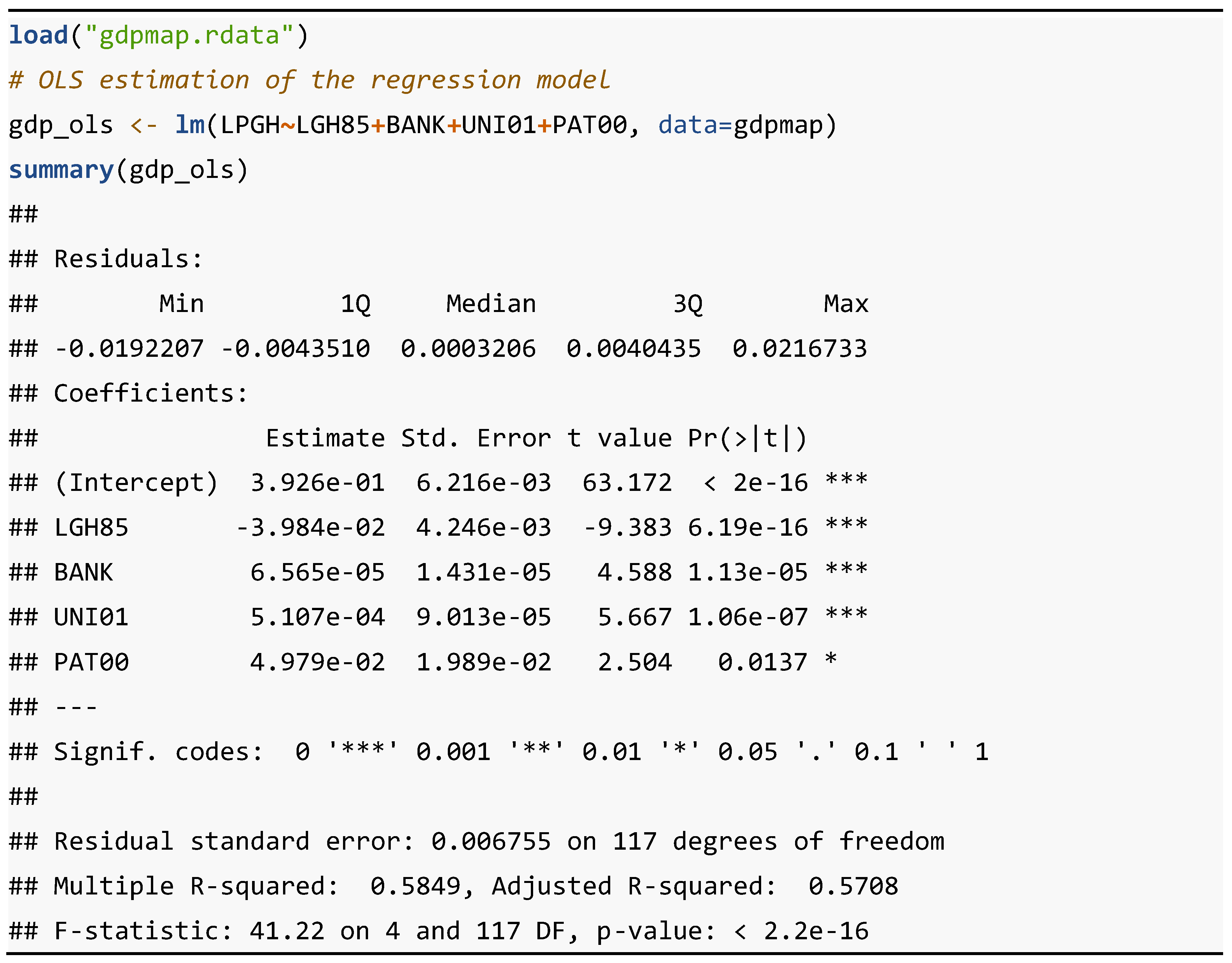
where y is the vector of the dependent variable, of order ( n × 1 ) ; X is the matrix of explanatory variables, of order ( n × k ) ; ι n is a vector of ones, of order ( n × 1 ) ; α ,   β are the set of ( k + 1 ) parameters to be estimated; and ε is the random disturbance variable, of order ( n × 1 ) , which is distributed as ε ~ N 0 , σ ε I n , where I n is the identity matrix of order n . This model is estimated by the Ordinary Least Squares (OLS) method. Table 12 presents the R code needed to generate the results of the OLS estimation of the basic linear regression model.
The following two libraries are required to run this code: "sp" and "stats". The main functions, not previously presented, involved in this R code are "lm" and "summary". lm {stats} is used to fit linear models, including multivariate ones. summary {base} is used to produce result summaries of the results of various model fitting functions.
The code sequences show how to estimate and test the model with a dataset of municipalities (NUTS 5) of the urban areas of Spain used in Mella and Chasco [16]. With these data, a model of urban economic growth is formulated in which the average rate of change of GDP per capita, in logarithms, over the period 1985-2003 (LPGH), is explained as a function of GDP per capita in 1985 logarithms (LGH85), the rate of change in the number of banking institutions in the period 1985-2003 (BANK), the percentage of people with secondary and university education out of the population aged 16 and over in 2001 (UNI01) and the rate of the number of patents per inhabitant in 2000 (PAT00). As can be seen, all estimators are statistically significant at least at 99% confidence. The model has an explanatory level of 58.49%.
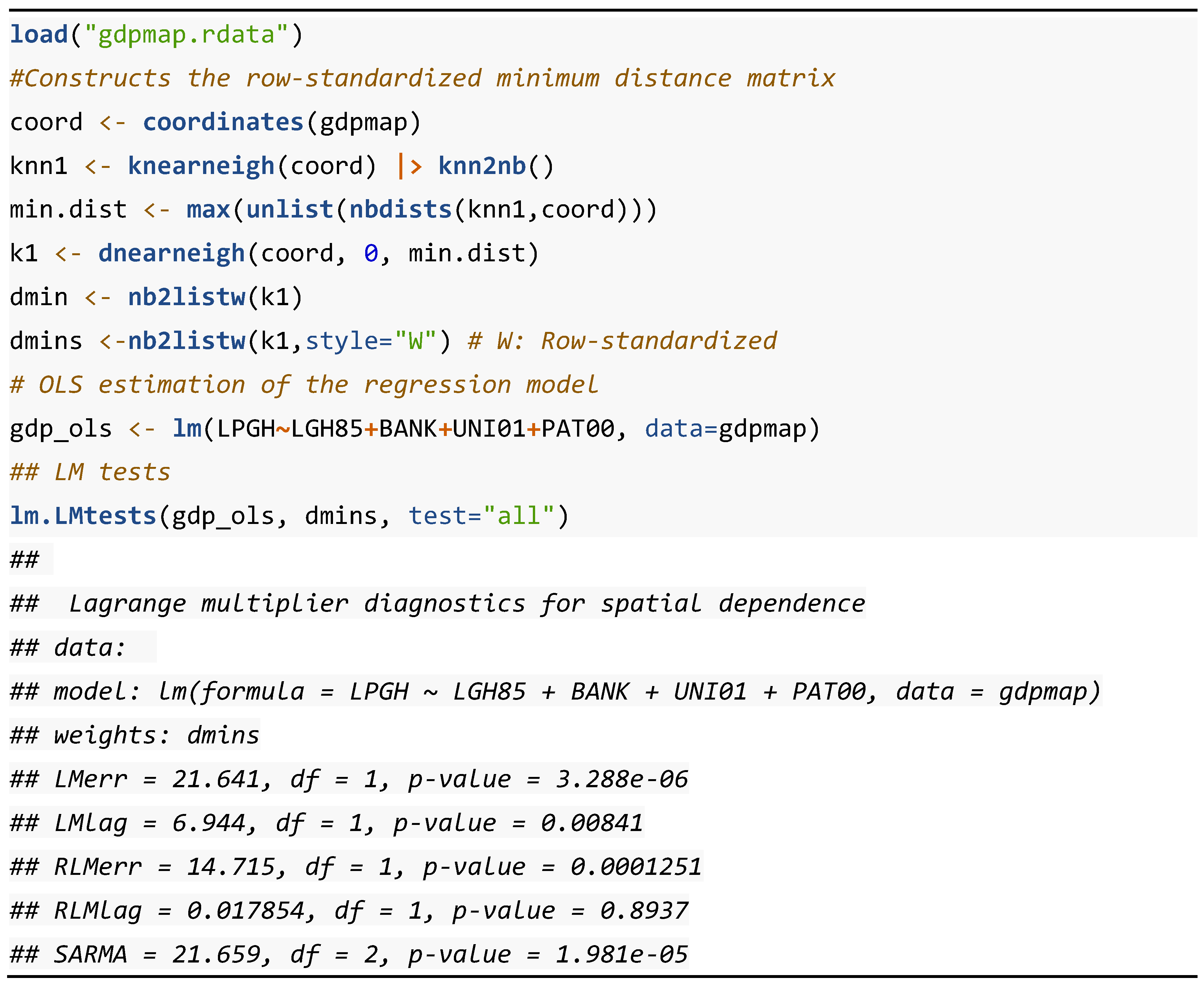
In order to test whether the variable of the OLS regression errors is spatially white noise,6 the Lagrange Multiplier (LM) tests are calculated on this variable. This basic hypothesis is rejected as soon as any of these tests, which are distributed as a Chi-square with 1 degree of freedom ( χ 1 2 ), is statistically significant. In particular, these tests are focused on a single alternative hypothesis. Thus, if the Lagrange multiplier test for the alternative hypothesis of spatially lagged dependent variable (LMLAG) is statistically significant instead of the Lagrange multiplier test for the alternative hypothesis of residual dependence (LMERR), the model that would best explain the data would be the spatial lag model or spatial autoregressive model of order 1 (SAR):
y = ρ W y + α ι n + X β + ε
being ρ a spatial autoregressive parameter to be estimated and W a row-standardised spatial weight matrix of order ( n × n ) . But if it is the LMERR test that is statistically significant, instead of the LMLAG, the best model would be the Spatial Error Model (SEM):
y = α ι n + X β + u u = λ W u + ε                
where λ is a spatial autoregressive parameter to be estimated. In this case, it should be noted that y = α ι n + X β + λ W u + ε and u = y α ι n X β . Therefore, the SEM would be equivalent to a spatial lag model that includes, on the right-hand side of the equation, in addition to the terms of the basic model, the spatially lagged dependent variable and the k spatially lagged explanatory variables as follows:
y = λ W y + α ι n + X β λ W X β + ε ;   for   θ = λ β
The restriction γ = λ β is called the common factor (COMFAC) hypothesis and when it holds, this model is called, by Anselin [8], as Spatial Durbin Model (SDM).
Regarding the LM tests previously presented, it is possible that both are statistically significant because, although they are tests oriented towards an alternative spatial hypothesis or model, they are also sensitive to the existence of the other type of spatial autocorrelation. In these cases, to decide on the most appropriate spatial model, spatial lag (SAR) or SEM, Anselin, Bera, Florax and Yoon [18] propose a solution by formulating robust versions of the LMLAG and LMERR tests, the new LMLE (a test to spatial lag dependence which is robust to ignored spatial error dependence) and LMEL (a test to spatial error robust to ignored spatial lag), respectively. If the values of LMLE > LMEL, the spatial lag (SAR) model should be selected, while if LMEL > LMLE, the SEM should be chosen.7
Table 13 presents the R code needed to generate the results of the computation of the LM test on the OLS estimation residuals. The following three libraries are required to run this code: "sp", "stats" and "spdep". The main functions, not previously presented, involved in this R code are "coordinates" and "lm.LMtest". coordinates {sp} retrieves spatial coordinates from a spatial object of class sp. lm.LMtest {spdep} reports the estimates of the LMERR test for error dependence (which is called ‘LMerr’ by the function), the LMLAG test for a missing spatially lagged dependent variable (‘LMlag’), their corresponding robust variants LMEL (‘RLMerr’) and LMLE (‘RLMlag’), respectively, and a SARMA test, which is test for a mixed residual spatial autoregressive process (SAR) and a spatial moving average (SMA).
The LMLAG and LMERR tests are both highly significant, so the null hypothesis of no spatial autocorrelation must be rejected with more than 99% confidence. Additionally, of the robust tests, it is only possible to reject the null hypothesis for LMEL (not for LMLE). Therefore, according to the classic modelling strategy, the most appropriate specification for this model would be the SEM.
Since the spatial lag model (SAR) includes as an explanatory variable the spatially lagged endogenous variable ( W y ) referred to the same moment in time as the dependent variable ( y ), a situation of simultaneity or contemporaneous dependence arises. Therefore, its estimation by OLS produces bias, inefficiency, and inconsistency in the estimators. As for the SEM, due to the heteroskedastic form of the variance and covariance matrix of the random disturbance u , its estimation by the OLS method results in inefficient, although consistent, estimators. Due to the problems of OLS in these spatial models, estimation by the Maximum Likelihood (ML) method in the case of normality in the OLS error variable is recommended as more appropriate (see Anselin [8], chap. 6).
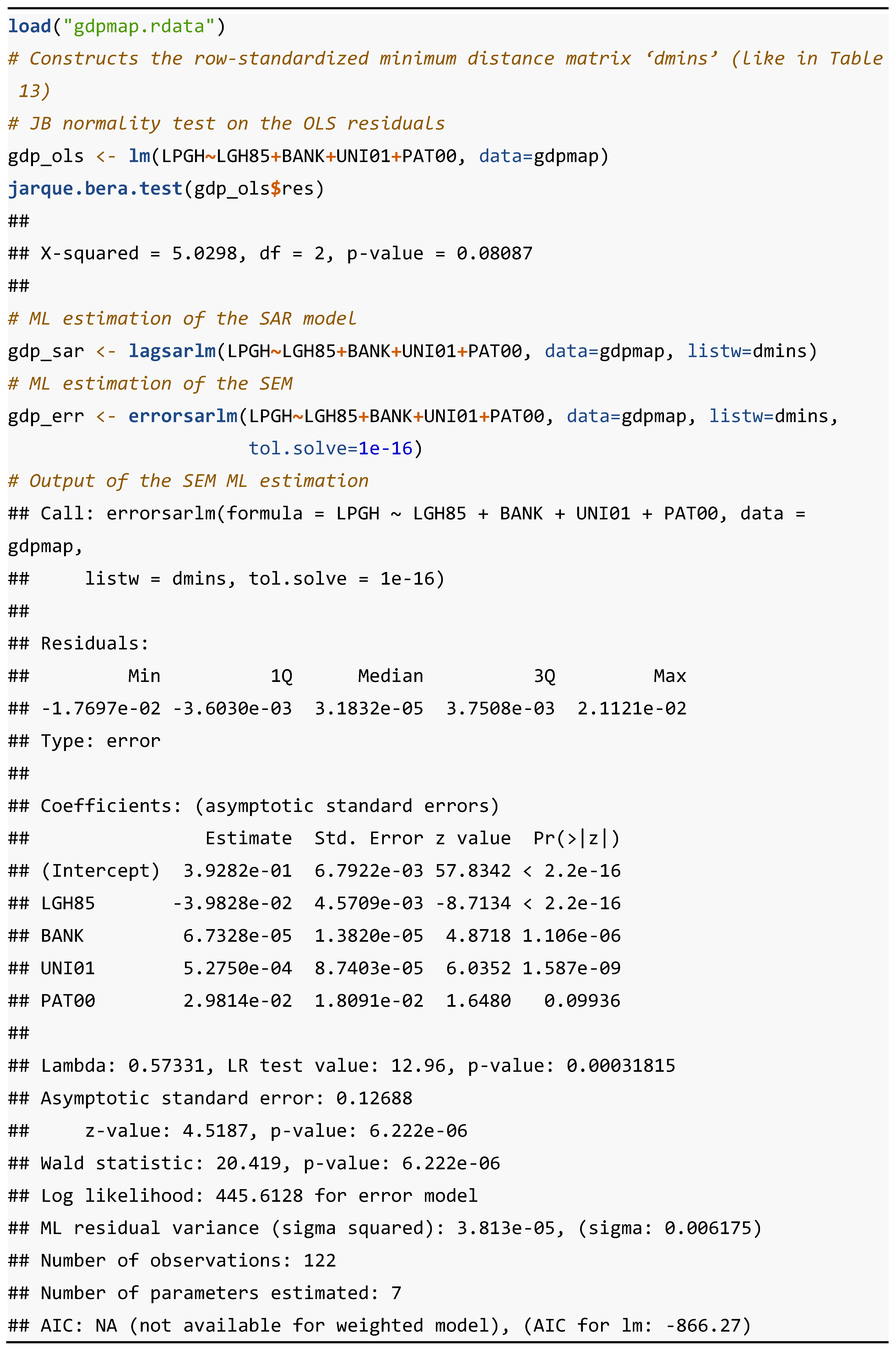
Table 14 presents the R code needed to generate the results of the ML estimations of the spatial lag (SAR) model and the SEM. The following four libraries are required to run this code: "sp", "stats", "spdep" and "tseries".
The main functions, not previously presented, involved in this code are "jarque.bera.test”, "lagsarlm" and "errorsarlm". jarque.bera.test {tseries} tests the null of normality for a variable using the Jarque-Bera test statistic). lagsarlm {spatialreg} provides ML estimation of spatial lag (SAR) models and SDM. errorsarlm {spatialreg} provides a ML estimation of SEM.
In Table 13, the LM tests on the OLS residuals showed the existence of spatial aucorrelation in the residuals and recommended the estimation of a SEM to correct for this problem. In Table 14, the Jarque-Bera test cannot reject the null hypothesis of normality of the OLS error terms with more than 95% confidence, so it is possible to estimate the SEM by the ML method. For this reason, only the results of this estimation in their entirety are presented in Table 14.
According to the STG strategy, the SEM is the model which best fits the data generation process. The value of the spatial autoregressive parameter λ = 0.57331 has no interpretation, unlike the spatial autoregressive ρ parameter, which is estimated in the spatial lag model (SAR). In fact, it is called by Anselin and Rey as a "nuisance" parameter and, therefore, no inference is performed for it ([17]). All estimators of the model are statistically significant although, with respect to the estimation of the basic model (Table 12), the estimator of the patent variable is only significant for a confidence level above 90%. In the case of the ML estimates, the R2, as a measure of goodness of fit, is not presented, but rather the ML and information criteria (Akaike and AIC).
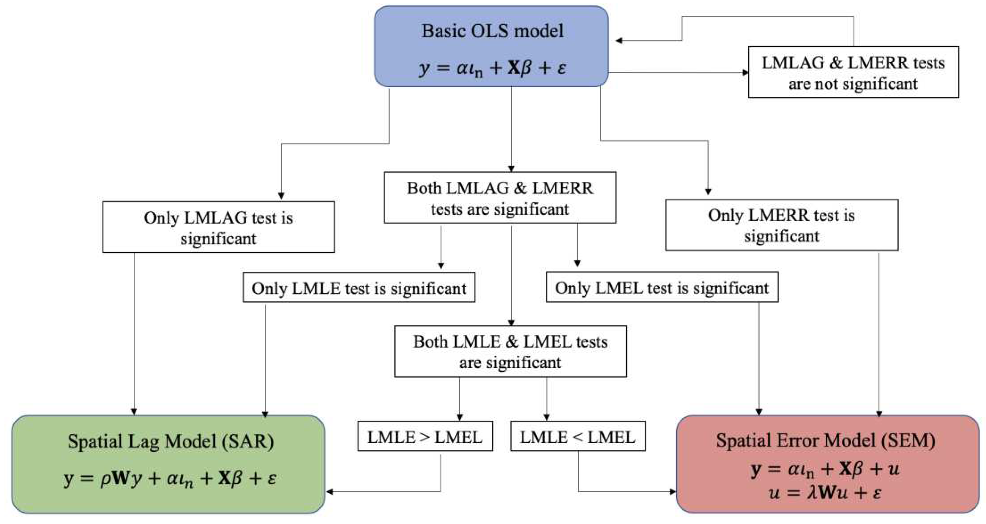
The modelling strategy proposed by Anselin and Rey ([17]) is presented in Figure 11.
When the OLS estimation errors follow a non-normal distribution, the spatial lag model (SAR) should be estimated by the Spatial Two-Stage Least Squares method (S2SLS) which, in the version of Kelejian and Robinson [20], consists of using the spatially lagged exogenous variables of several orders of contiguity as instruments of the spatially lagged endogenous variable, resulting in a consistent, though not very efficient, autoregressive estimator ( ρ ^ ).
As for the SEM, Arraiz, Drukker, Kelejian and Prucha [21] present an estimation by the General Method of Moments (GMM), building on the initial proposal made by Kelejian and Prucha [22]. Although, given that the estimators are unbiased and consistent, it is also considered acceptable to estimate the SEM by OLS by performing robust inference of the variance-covariance matrix of the estimators by the KP-HET method proposed by Kelejian and Prucha [23], which takes into account the joint existence of heteroscedasticity and spatial autocorrelation in the regression errors.
Table 15 presents the R code needed to generate the results of the STSLS and GMM estimations of the spatial lag (SAR) model and the SEM, respectively. The following three libraries are required to run this code: "sp", "spdep" and "spatialreg".
The main functions, not previously presented, involved in this R code are ""stsls" and "GMerrorsar". stsls {spatialreg} fits a spatial lag model (SAR) by STSLS. GMerrorsar {spatialreg} fits a SEM by the Kelejian and Prucha’s GMM.

3.1.2. LeSage’s General-To-Specific Strategy (GTS)

The second strategy, GTS, is to start from the most general spatial autocorrelation model possible. According to Manski [24], this general model is the one that includes the three possible types of spatial interaction, endogenous ( W y ), exogenous ( W X ) and unobserved ( W u ) effects:
y = ρ W y + α ι n + X β + W X θ + u u = λ W u + ε                                                                              
where θ is a vector of k spatial autoregressive parameters. The problem with this Manski’s model is that, as the author demonstrates, it is impossible to identify its parameters. Therefore, it is necessary to reduce the three types of spatial interaction to two, which gives rise to three possible general sub-models of spatial autocorrelation. First, if we exclude the spatial endogenous effect ( ρ = 0 ), we obtain the so-called, by LeSage and Pace [25], Spatial Durbin Error Model (SDEM):
y = α ι n + X β + W X θ + u u = λ W u + ε                                                
Secondly, if what is excluded is the spatial exogenous effect (( θ = 0 ), the SARAR model or Kelejian-Prucha’s model is obtained, as it was proposed by these authors ([22])8:
y = ρ W y + α ι n + X β + u u = λ W u + ε                                          
Finally, if the spatial unobserved effect is excluded, we obtain the unconstrained Spatial Durbin Model (SDM), where the constraint presented in Equation (11) do not hold; that is, when θ λ β . Hence:
y = ρ W y + α ι n + X β + W X θ + ε
As with the SAR model, the presence of the spatial lag of the dependent variable on the right-hand side of the equation does not result in OLS estimators with good properties, so this model must be estimated by ML.
This is the general model proposed by LeSage and Pace [25] as a starting point for the GTS modelling strategy.9 The SDM model fulfils the identifiability condition by including two of the three possible types of spatial interaction, endogenous and exogenous effects, and thus includes all spatially lagged explanatory variables. In this way, a possible bias in the estimators caused by the omission of any relevant spatial variable is avoided.
Additionally, LeSage and Pace demonstrated that if this model also had residual spatial autocorrelation problems, the omission of the spatially lagged error variable would lead to inefficiency, but not to bias in the estimators. The SDM model likewise has the property of nesting several models, from the basic model without spatial effects to the SAR and SEM spatial autocorrelation models (when the COMFAC hypothesis is satisfied), as well as the so-called, by LeSage and Pace [25], Spatial Lag of X (SLX) model, firstly called “mixed regressive-spatial cross-regressive model” by Florax and Folmer [27].
y = α ι n + X β + W X θ + ε
This model can be estimated by the OLS method since, if the explanatory variables are exogenous, their corresponding spatial lags will also be exogenous. In addition, the SLX model has two more good properties: on the one hand, it is more flexible to estimate or parameterise the W matrix and, on the other hand, it has better properties to capture spatial spillover effects when no clear theoretical model is available to support the inclusion of the endogenous spatial interaction effect ( W y ), as shown by Halleck Vega and Elhorst [28].
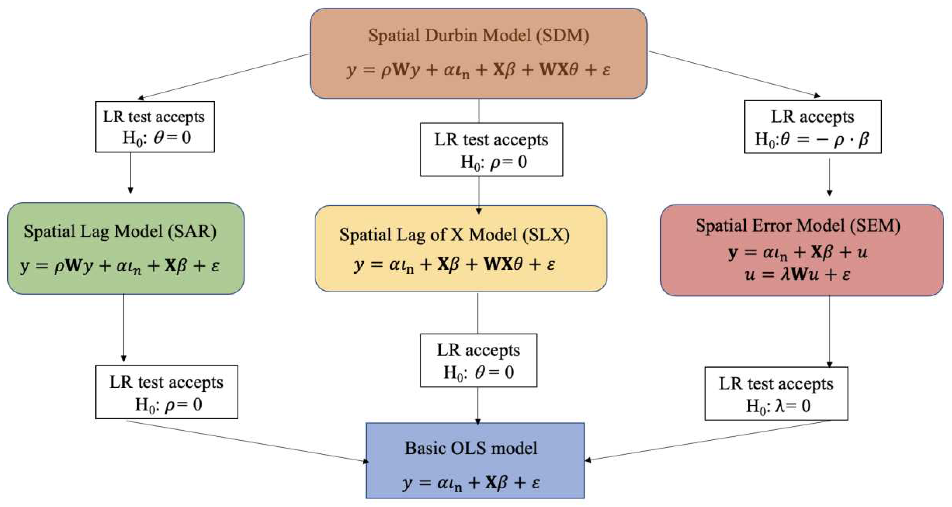
The modelling strategy proposed by LeSage and Pace ([25]) is presented in Figure 12.
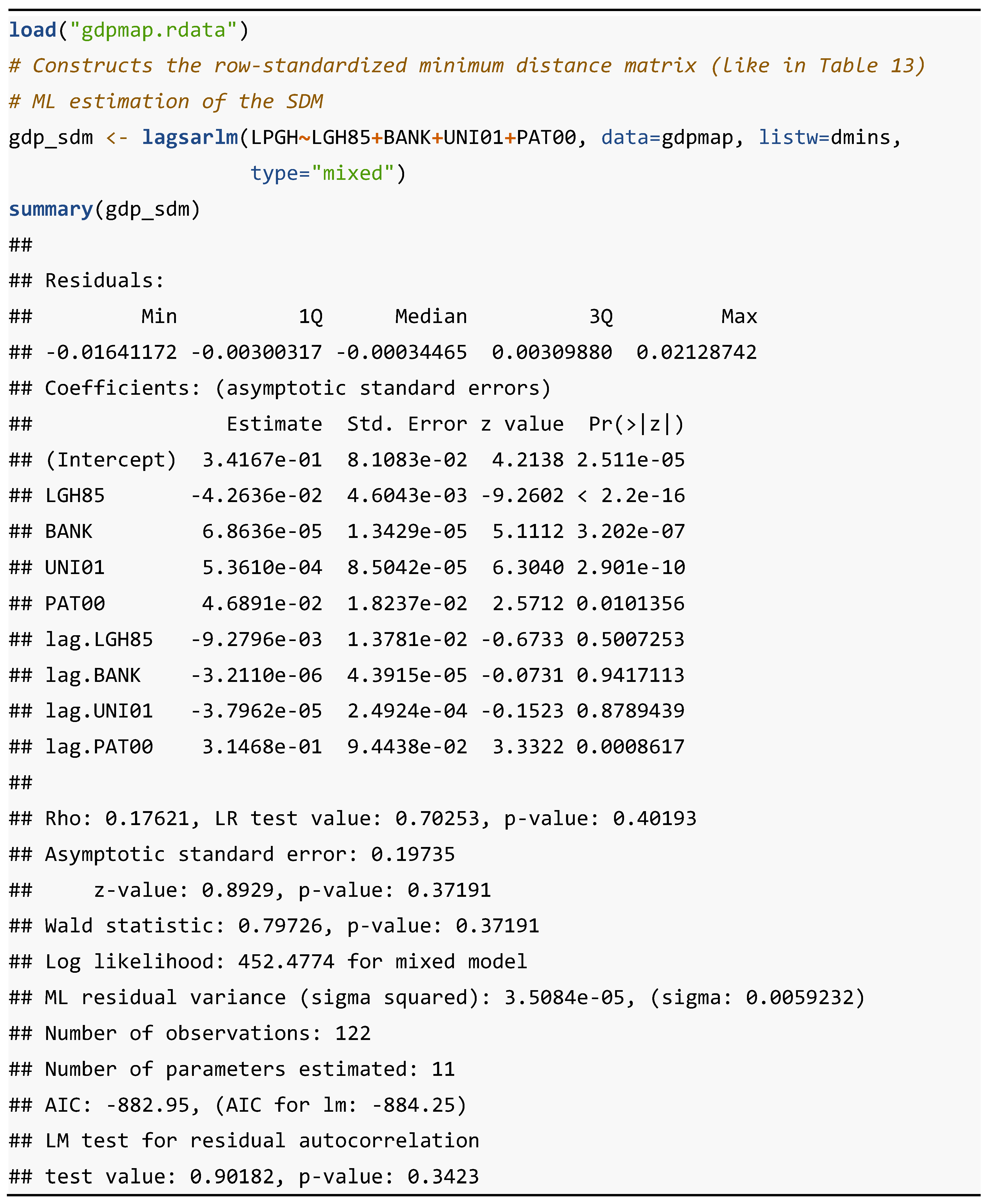
Table 16 presents the R code needed to generate the results of the ML estimation of the SDM model. The following three libraries are required to run this code: "sp", "spdep" and "spatialreg". In this case, there are no new functions.
In the output, the estimation results highlight the contrast between the high statistical significance of the model's explanatory variables and the low significance of their corresponding spatial lags. The only exception is the patent variable and its corresponding spatially lagged variable, for which both coefficients are highly significant, especially in the case of the latter.
However, the lack of statistical significance of the autoregressive coefficient ρ ^ (p-value: 0.40193) is striking, raising doubts about the suitability of this identification as the most appropriate for the model. Finally, the function also calculates an LM test on the residuals of this regression, which is not significant, demonstrating the non-existence of spatial autocorrelation in the residuals.
As can be seen in Figure 12, the decision on the most appropriate model for the data generating process, according to this GTS strategy, requires the calculation of several Likelihood Ratio (LR) tests, which will be discussed in more detail in the next section, where we will present a hybrid strategy, which combines the two strategies seen so far: STG and GTS.

3.1.3. Elhorst’s Hybrid Strategy

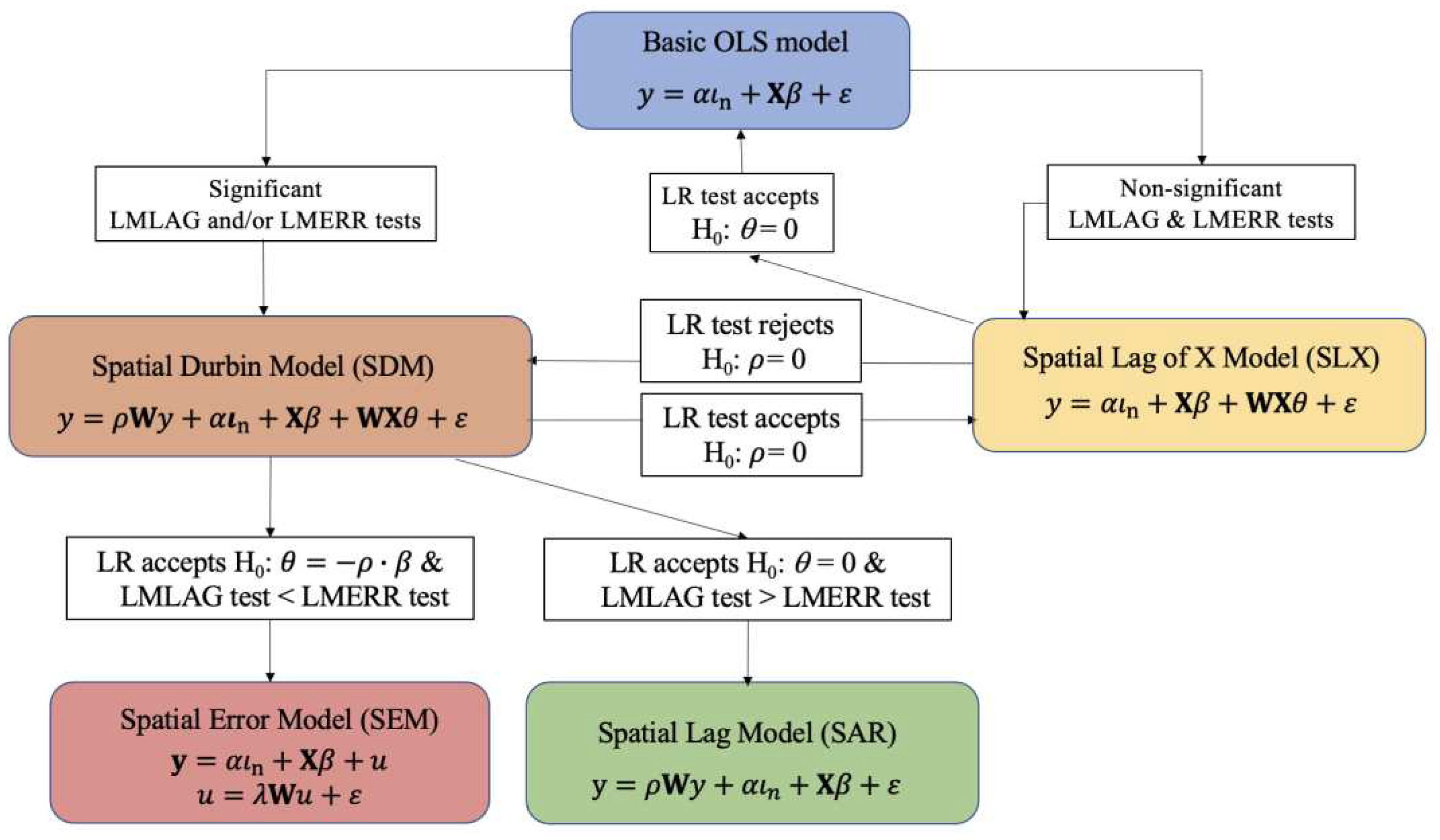
Based on the two previous approaches, Elhorst [29] proposes a hybrid strategy, which takes into account the good properties of both proposals. For this reason, this strategy will be the one we select as the most suitable for identifying spatial autocorrelation models. As presented in Figure 13, the Elhorst’s hybrid strategy starts, like the STG strategy, with the OLS estimation of a basic model without spatial effects. The error variable of this regression is analysed with the LMLAG and LMERR tests, to check whether they are white noise. At this point, it may happen that one of the tests is statistically significant or that none of them is. Firstly, if any of the LM tests is significant, it is recommended to select the SDM model, as proposed by the GTS strategy.
The ML estimation of this model allows the likelihood ratio (LR), whose distribution follows a Chi-square with k degrees of freedom ( χ k 2 ), to be used to test the null hypotheses H 0 θ = 0 and H 0 θ = ρ · β . If the second (COMFAC) hypothesis cannot be rejected, the SDM should be simplified to a spatial lag (SAR) model, provided that the LMLAG > LMERR tests. If the first hypothesis cannot be rejected, the SEM should be selected, provided that LMERR > LMLAG tests. If there is no agreement between the results of the LR test and the LM tests, then the SDM would be the model that best describes the data.
Secondly, if after the OLS estimation of the basic model none of the LM tests is statistically significant, then the basic model would have to be re-estimated as an SLX model, including all spatially lagged exogenous variables or a subset of them, in order to test the null hypothesis H 0 θ = 0 . If this hypothesis cannot be rejected, the basic model should be chosen as the one that best describes the data, i.e., there would be no evidence of the need for spatial autocorrelation effects to explain the dependent variable. But if, on the contrary, the hypothesis H 0 θ = 0 can be rejected, the SDM model would have to be estimated to test, again, the null hypothesis H 0 ρ = 0 . If this hypothesis can be rejected, the selection would be the SDM; on the contrary, it should be settled that a model with spatially lagged independent variables (complete or parsimonious SLX) only suffices.
Additionally, Halleck Vega and Elhorst [28] introduced the SLX model into the model selection process as a new SDM’s nested model (like in Figure 12), recommending its choice when the null hypothesis H 0 ρ = 0 cannot be rejected. This addition may lead to differences in the final model selected, as will be seen below.
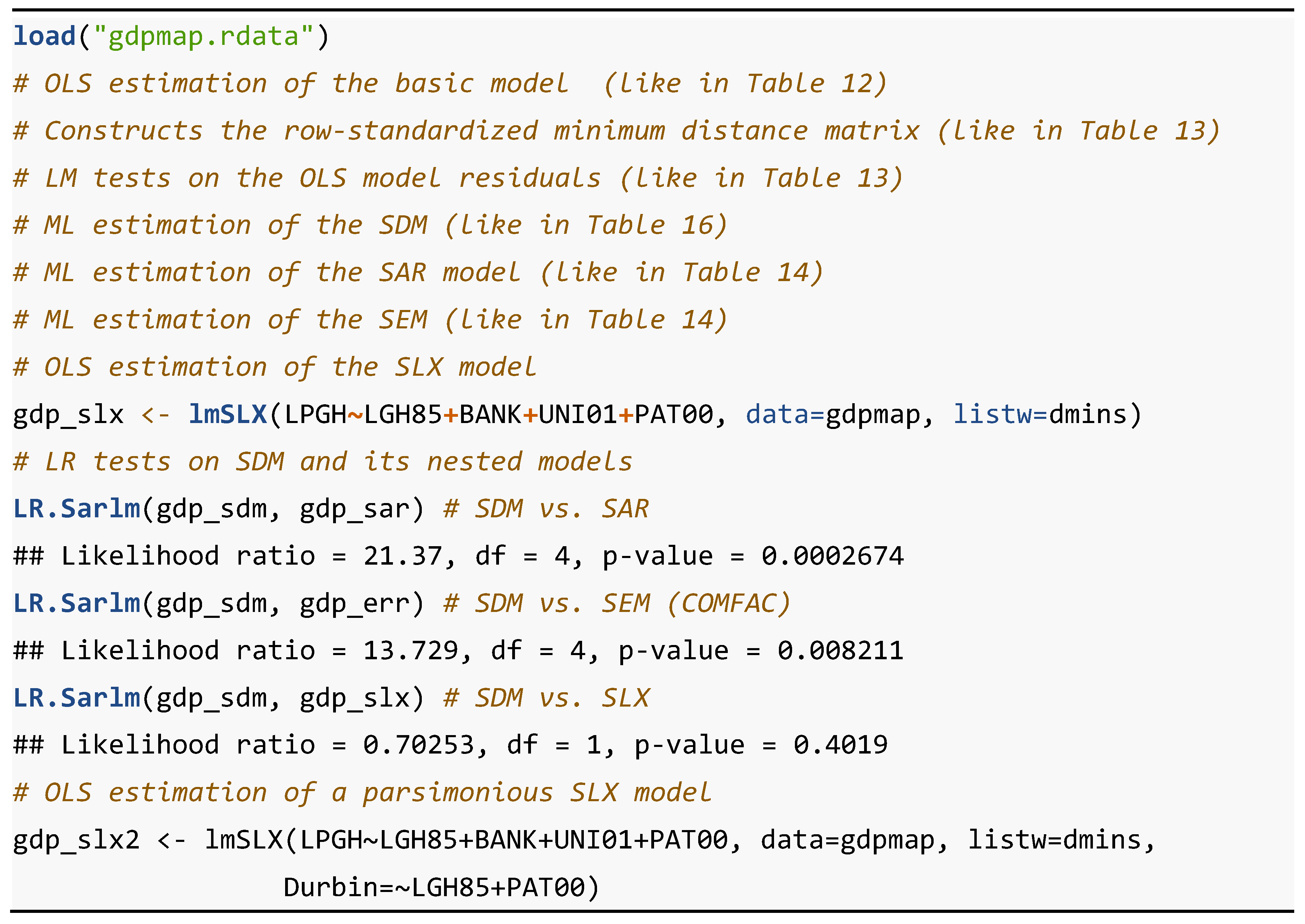
Table 17 presents the R code needed to compute the LM and LR tests necessary to determine the best model specification according to the Elhorst’s hybrid strategy. The following four libraries are required to run this code: "sp", "stats", "spdep" and "spatialreg". The main functions, not previously presented, involved in this R code are "lmSLX" and "LR.Sarlm". lmSLX {spatialreg} fits a SLX model, i.e., an OLS model augmented with the spatially lagged regressor variables. LR.Sarlm {spatialreg} is a function which provides a likelihood ratio test.
As seen in the results of the classical strategy (Table 13), the LM tests on the OLS residuals are both statistically significant, with LMLAG < LMERR. Therefore, the SEM was identified as the most appropriate specification for the urban growth model. However, according to Elhorst's hybrid strategy, the significance of any or all of the LM tests involves estimating the SDM and then comparing it with the LR tests of their corresponding more restricted nested models. In his first version in 2010 [29], Elhorst proposes to compare the SDM with the spatial lag model (SAR) and the SEM. As can be seen in Table 17, the null hypothesis of the fulfilment of the COMFAC hypothesis, H 0 θ = ρ · β , and the null hypothesis of H 0 θ = 0 must be rejected. In other words, the most appropriate specification for the model is the SDM. However, if SLX is incorporated into the comparison of rival models, which is what Elhorst does in his second formulation in 2015 [28], the null hypothesis H 0 ρ = 0 cannot be rejected. Therefore, the more appropriate specification for the data-generating process would be the SLX model, rather than the SDM.10 Specifically, a more parsimonious SLX model is selected that only includes, as explanatory variables, the spatially lagged variables that are statistically significant, as shown in the last rows of the Table 17.
Therefore, the selection of the most appropriate final model is still an open question since, as we have seen, the outcome depends on the modelling strategy adopted. In the proposed example of urban growth in Spain, if the Anselin’s classical STG strategy is followed, the selected model would be the SEM. According to the original proposal of Elhorst's hybrid strategy, the proposed model would be the SDM. Finally, according to Elhorst's second proposal, and also LeSage and Pace's GTS strategy, the model finally selected would be the SLX.
All these models must be estimated by the OLS and ML methods to be able to use the LR as a testing tool, although it should be noted that spatial autocorrelation models can also be estimated with Bayesian methodology using the Markov Chains Monte Carlo (MCMC) approach, as explained in LeSage and Pace [25], chapter 5.
To conclude this section on the identification of true data generation process of a dependent variable, it must be said that there is still a long way to go to create a method that considers not only the existence of the spatial autocorrelation effect, but also spatial heterogeneity, as shown by Debarsy and Le Gallo [30]. Spatial heterogeneity can manifest itself in various forms, such as diversity of coefficients or of the functional relationships themselves in various locations or groups of locations (spatial regimes), spatial clustering, hierarchical structures, etc. But this is a topic that will not be dealt with in this paper.
3.2. Interpretation of the Estimators of Spatial Autocorrelation Models

Only in spatial autocorrelation models where the endogenous effect ( W y ) is not present in the right-hand side of the model, can the estimated coefficients ( β ^ ) be interpreted directly, as in the basic model without spatial effects, because the reduced form coincides with the structural form. Of the specifications presented above, this would be the case for the basic OLS model, the SDEM and the SLX model. That is, the marginal effect of a change in the value of a continuous explanatory variable for a given location coincides with the value of the estimator corresponding to that variable:
y i x i , k = β k
In all other cases, the correct interpretation of the estimators involves first moving from the structural form to the reduced form. Thus, for example, in the spatial lag (SAR) model of Equation (9) the reduced form would be (under certain invertibility conditions):
y = I ρ W 1 α ι n + X β + ε
The term I ρ W 1 is called the spatial multiplier and, using the potential expansion, can also be expressed as follows:
I ρ W 1 = I + ρ W + ρ 2 W 2 + ρ 3 W 3 +
If this new expression is used in Equation (18), for the conditional mean, the value of y at a given location i is a function of not only the value of the explanatory variables at that location, but also of the value of the explanatory variables at neighbouring locations (through the term ρ W X β ), of the value of the explanatory variables at neighbours’ neighbours (through the term ρ 2 W 2 X β ), etc.
E y | X = X β + ρ W X β + ρ 2 W 2 X β + ρ 3 W 3 X β +
Therefore, if we restrict our analysis to the relationship between the variable y as a whole and a given variable x k of the matrix X , the marginal effect of a change in all the values of the column vector x k on all the values of y would be as follows:
y x k ' = x k β k + ρ W x k β k + ρ 2 W 2 x k β k + ρ 3 W 3 x k β k + x k '
Unlike the marginal effect obtained for the basic model (Equation 17), the result of this expression does not refer to a given location i , but to all of them as a whole, and it is not a scalar ( β k ) either, but a matrix of order n × n . If we now calculate the effect of discrete changes in the elements of x k on the values of y :
Δ y = Δ x k β k + ρ W Δ x k β k + ρ 2 W 2 Δ x k β k + ρ 3 W 3 Δ x k β k +
As can be seen in the right-hand side of the equation, the total effect on the values of the dependent variable and of changes in the values of an explanatory variable, x k , is the result of a direct effect (first summand) plus an indirect effect from the spatial multiplier (remaining summands). From this expression, two types of analysis can be distinguished, one particular and the other general.
First, Anselin and Rey [17] analyse the particular case of the total effect produced by a unit change of x k , in all the locations at the same time, on each and every value of y , which would be equal to a scalar, β k / 1 ρ . This is the result of a direct effect ( β k ) plus an indirect effect driven by the spatial multiplier, ( β k · ρ / 1 ρ ). As explained by these authors, this expression can be used to simulate the total effects of certain changes in an explanatory variable on all the observations of the dependent variable.
Second, LeSage and Pace [25] present the more general case of the effects caused by the change in the value of "one" location, j , of the variable x k on "another" location, i , of the variable y . Here, each effect is no longer a scalar, but a complete matrix, S k W i j , of order n × n . That is, each explanatory variable x k in the model will have its own full matrix of impacts on the dependent variable.
S k W i j = y i x j k ' = I n ρ W 1 β k
In this case, we can also distinguish between direct and indirect effects. The direct effect would be the effect caused by changes in the value of x k , at location i on the value of y at that same location i . These effects constitute the values of the main diagonal of the matrix S k W i i . The indirect effect is constituted by the rest of the values of the matrix S k W i j , which would be the "feedback loops" in which the value of x k , in a location j affects the value of y in location i , and vice versa, being possible longer runs in which the effect in one location could reach the last observation n of the spatial system, and then go back to the starting point.
For example, the value of S k W 11 would mean the direct effect of a change in the value of variable x k at location 1 ( x 1 , k ) on the value of variable y at location 1 ( y 1 ), while the value of S k W 13 would be the indirect effect of a change in the value of variable x 1 , k on the value of variable y at location 2 (y_2). In the rows, the matrix S k W i j has the effects of x k from each location i "to" every one of the locations j , while the columns represent the effect on each location j "from" every one of the locations i .
Since it is not possible to construct an inferential process for all impacts in the matrix S k W i j , LeSage and Pace propose to make the inference on the mean value of the direct and total effects, extracting the indirect effects by difference:
Preprints 84347 i001
In LeSage and Pace [25], chapter 2, the same process and results for the more complex SDM are laid out.
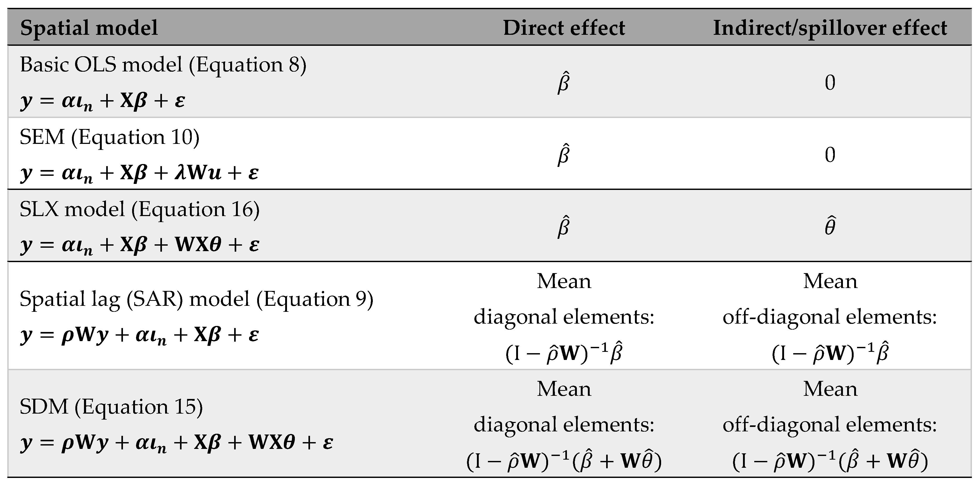
Therefore, the interpretation of the coefficients in spatial autocorrelation models is not always equivalent to the coefficient estimated by the regression, β ^ , and it is first necessary to express the model in its reduced for to identify the correct mathematical expression. Moreover, it is also typical of some of these models that, in addition to the direct effect caused by unit variations in the independent variables on the dependent variable, in each observation, there is an indirect or spillover effect from variations in neighbouring units. Therefore, each explanatory variable produces a total effect on the explanatory variable that is the sum of the two previous ones. As explained by Halleck Vega and Elhorst [28], the spillover effect cannot be observed in some spatial dependence models, such as the SEM. The spillover effect is also absent in the basic OLS model because of the implicit assumption that outcomes for different observations are independent of each other. In summary, in a similar way to that used by the authors, we present these effects, for the models used in this paper:
Table 18. Direct and spillover effects corresponding to different model specifications.
Preprints 84347 t018
Source: Elaborated from Halleck Vega and Elhorst [28], Table 1.
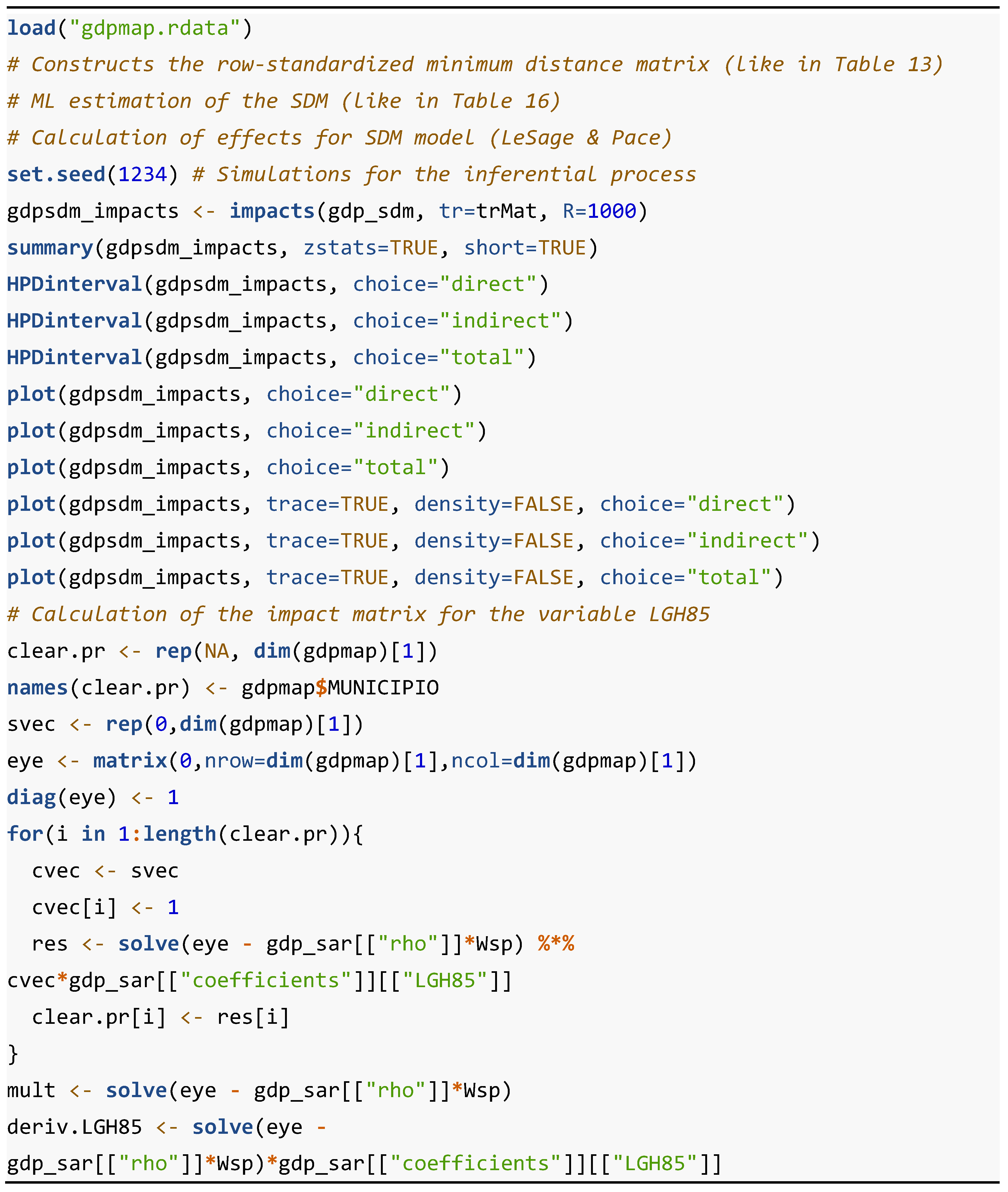
Table 19 presents the R code needed to calculate the direct, indirect, and total effect matrices, as well as the inference and the impact matrix of an explanatory variable for the SDM model, in the case of the model of urban economic growth in Spain. The following four libraries are required to run this code: : "sp", " spdep", " spatialreg" and "coda", which provides functions for summarizing and plotting the output from Markov Chain Monte Carlo (MCMC) simulations. The main functions, not previously presented, involved in this R code are "as_dgRMatrix_listw", "trW", "set.seed", "impacts", "HPDinterval", "rep", "names", "matrix" "diag" and "solve".
as_dgRMatrix_listw {spatialreg} converts a weights list to a sparse matrix class object. trW {spatialreg} is used to prepare a vector of traces of powers of a spatial weight matrix. set.seed {base} is the recommended way to specify seeds. impacts {spatialreg} calculates the impacts for spatial lag (SAR) and SDM. HPDinterval {coda} Create Highest Posterior Density (HPD) intervals for the parameters in MCMC sample. rep {base} replicates elements of vectors and lists. names {base} gets or sets the names of an object. matrix {base} creates a matrix from the given set of values. diag {base} extract or replace the diagonal of a matrix or construct a diagonal matrix. solve {base} solves a system of equations.
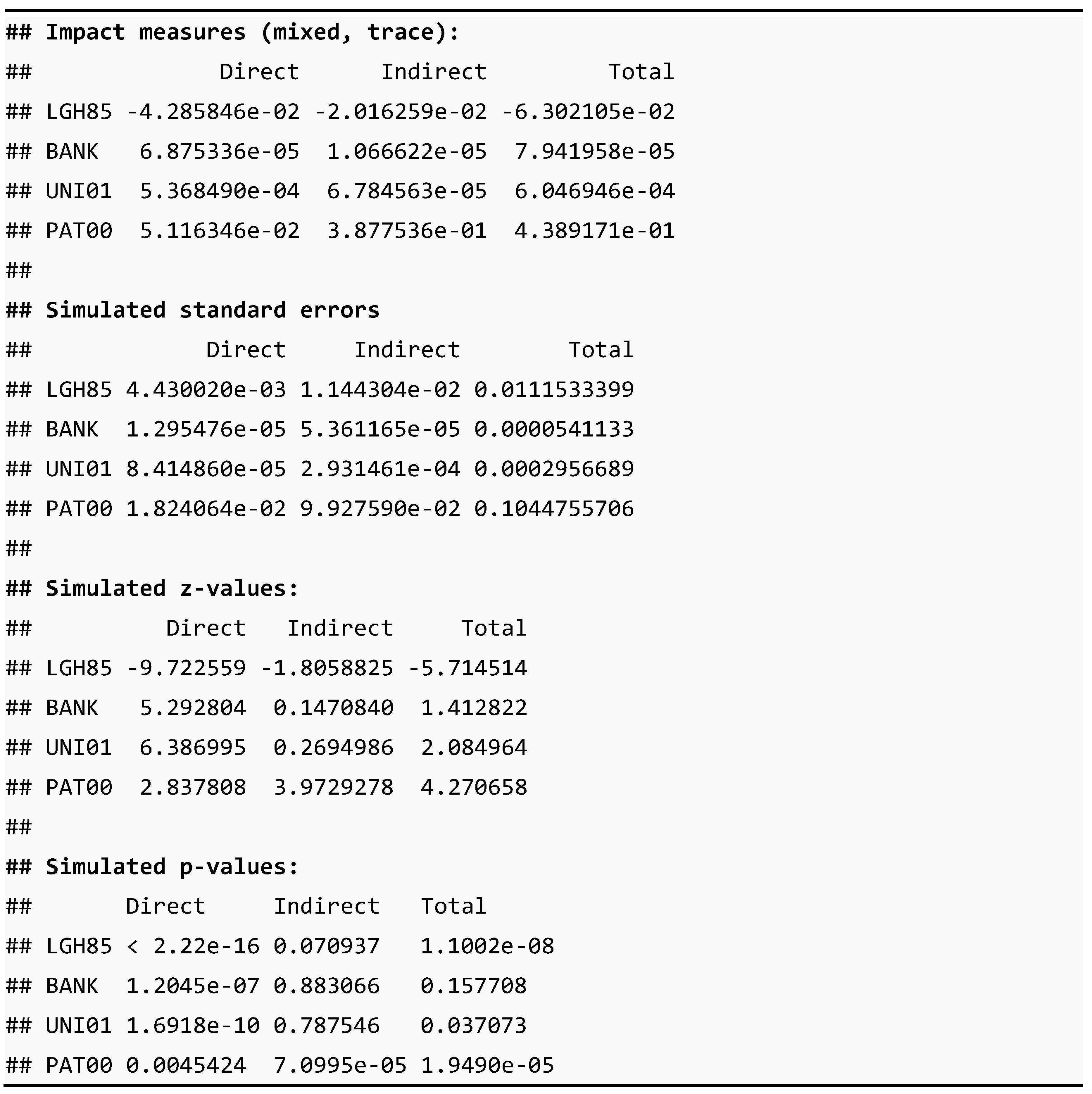
The output of the calculation of the effects for the SDM model is presented in Table 20.
Table 20 shows that the model estimates are -practically all- statistically significant and, except in the case of the LGH85 variable, they are positive. The negative sign of the coefficient of LGH85 demonstrates the existence of income convergence in the group of large Spanish cities. The total impact of a 10% growth in GDP per capita in a city in the initial period (1985) implied a fall in the average rate of change of GDP per capita in the period 1985-2003 of -0.63% in that city. This impact is the sum of the direct effect caused by the growth of GDP per capita in the city itself (-0.43), which is the direct effect, and the indirect effect coming from the growth of GDP per capita in the rest of the cities (-0.20). Additionally, the total effect of the growth of 1 patent per inhabitant led to a growth of GDP per capita in the period of 0.44%, of which 0.05% came from the growth of patents per capita in the city itself (direct effect) and the remaining 0.39% was caused indirectly by the growth of patents in the rest of the cities.

4. Conclusions

This paper introduces the spatial component in econometric estimation and, in particular, the spatial dependence effect inherent in some of the variables involved in the modelling process, first, the spatial structure of the data is observed from maps, and the Moran’s spatial autocorrelation indicator is presented. Then, the spatial weights matrix is constructed under different specifications. Finally, the taxonomy of spatial econometric models is shown, the hybrid specification strategy is presented, and the interpretation of the estimated coefficients ends.

Author Contributions

Conceptualization, A.V. and C.C; methodology, A.V. and C.C.; software, A.V. and C.C.; validation, A.V. and C.C.; formal analysis, A.V. and C.C.; investigation, A.V. and C.C.; resources, A.V. and C.C.; data curation, A.V. and C.C; writing—original draft preparation, A.V and C.C..; writing—review and editing, A.V. and C.C.; visualization, A.V. and C.C. Authors have read and agreed to the published version of the manuscript.

Data Availability Statement

The data and scripts are available in the Spatial and Regional Economics research group (ECONRES) of the Universidad Autónoma de Madrid and the following repository: [6].

Conflicts of Interest

The authors declare no conflict of interest.

Appendices

A.1. R Code: Spatial Autocorrelation Patterns (Figure 1)

Preprints 84347 g014Preprints 84347 g015

References

  1. Lefebvre, H. The Production of Space; Wiley-Blackwell: Oxford (UK) & Cambridge (USA), 1992; ISBN 978-0-631-18177-4. [Google Scholar]
  2. Tobler, W.R. A Computer Movie Simulating Urban Growth in the Detroit Region. Econ. Geogr. 1970, 46, 234–240. [Google Scholar] [CrossRef]
  3. Bivand, R.S. Exploratory Spatial Data Analysis. In Handbook of Applied Spatial Analysis: Software Tools, Methods and Applications; Fischer, M.M., Getis, A., Eds.; Springer: Berlin, Heidelberg, 2010; pp. 219–254. ISBN 978-3-642-03647-7. [Google Scholar]
  4. Friendly, M. A.-M. Guerry’s “Moral Statistics of France”: Challenges for Multivariable Spatial Analysis. Stat. Sci. 2007, 22, 368–399. [Google Scholar] [CrossRef]
  5. Anselin, L. A Local Indicator of Multivariate Spatial Association: Extending Geary’s c. Geogr. Anal. 2019, 51, 133–150. [Google Scholar] [CrossRef]
  6. Chasco, C.; Vallone, A. Introduction to Cross-Section Spatial Econometric Models with Applications in R [Data and Codes] 2023, B2SHARE, EUDAT Repository, EU, 1 file, 840.4 kB. [CrossRef]
  7. Monmonier, M. How to Lie with Maps, Third Edition; University of Chicago Press: Chicago, IL, 2018; ISBN 978-0-226-43592-3. [Google Scholar]
  8. Anselin, L. Spatial Econometrics: Methods and Models; Springer Science & Business Media, 1988; ISBN 978-90-247-3735-2. [Google Scholar]
  9. Martori, J.C.; Hoberg, K.; Madariaga, R. La Incorporación Del Espacio En Los Métodos Estadísticos: Autocorrelación Espacial y Segregación. In Proceedings of the Conference: Actas del X Coloquio Internacional de Geocrítica; Barcelona, Spain, May 30 2008. [Google Scholar]
  10. Bivand, R.S.; Wong, D.W.S. Comparing Implementations of Global and Local Indicators of Spatial Association. TEST 2018, 27, 716–748. [Google Scholar] [CrossRef]
  11. Vallone, A.; Chasco, C. Spatiotemporal Methods for Analysis of Urban System Dynamics: An Application to Chile. Ann. Reg. Sci. 2020, 64, 421–454. [Google Scholar] [CrossRef]
  12. Pebesma, E.; Bivand, R.; Racine, E.; Sumner, M.; Cook, I.; Keitt, T.; Lovelace, R.; Wickham, H.; Ooms, J.; Müller, K.; et al. Sf: Simple Features for R 2023.
  13. Anselin, L.; Bera, A.K.; Florax, R.; Yoon, M.J. Simple Diagnostic Tests for Spatial Dependence. Reg. Sci. Urban Econ. 1996, 26, 77–104. [Google Scholar] [CrossRef]
  14. Chasco, C. Econometría Espacial Aplicada a La Predicción-Extrapolación de Datos Microterritoriales; Consejería de Economía e Innovación Tecnológica, Comunidad de Madrid: Madrid, 2003; ISBN 978-84-451-2442-0. [Google Scholar]
  15. Anselin, L. Local Indicators of Spatial Association—LISA. Geogr. Anal. 1995, 27, 93–115. [Google Scholar] [CrossRef]
  16. Mella, J.M.; Chasco, C. Urban Growth and Territorial Dynamics: A Spatial-Econometric Analysis of Spain. In Spatial Dynamics, Networks and Modelling; Edward Elgar Publishing, 2006; ISBN 978-1-78100-747-1. [Google Scholar]
  17. Anselin, L.; Rey, S.J. Modern Spatial Econometrics in Practice: A Guide to GeoDa, GeoDaSpace and PySAL; GeoDa Press LLC, 2014; ISBN 978-0-9863421-0-3. [Google Scholar]
  18. Anselin, L.; Bera, A.K.; Florax, R.; Yoon, M.J. Simple Diagnostic Tests for Spatial Dependence. Reg. Sci. Urban Econ. 1996, 26, 77–104. [Google Scholar] [CrossRef]
  19. Mur, J.; Angulo, A. Model Selection Strategies in a Spatial Setting: Some Additional Results. Reg. Sci. Urban Econ. 2009, 39, 200–213. [Google Scholar] [CrossRef]
  20. Kelejian, H.H.; Robinson, D.P. A Suggested Method of Estimation for Spatial Interdependent Models with Autocorrelated Errors, and an Application to a County Expenditure Model. Pap. Reg. Sci. 1993, 72, 297–312. [Google Scholar] [CrossRef]
  21. Arraiz, I.; Drukker, D.M.; Kelejian, H.H.; Prucha, I.R. A Spatial Cliff-Ord-Type Model with Heteroskedastic Innovations: Small and Large Sample Results*. J. Reg. Sci. 2010, 50, 592–614. [Google Scholar] [CrossRef]
  22. Kelejian, H.H.; Prucha, I.R. A Generalized Spatial Two-Stage Least Squares Procedure for Estimating a Spatial Autoregressive Model with Autoregressive Disturbances. J. Real Estate Finance Econ. 1998, 17, 99–121. [Google Scholar] [CrossRef]
  23. Kelejian, H.H.; Prucha, I.R. Specification and Estimation of Spatial Autoregressive Models with Autoregressive and Heteroskedastic Disturbances. J. Econom. 2010, 157, 53–67. [Google Scholar] [CrossRef] [PubMed]
  24. Manski, C.F. Identification of Endogenous Social Effects: The Reflection Problem. Rev. Econ. Stud. 1993, 60, 531–542. [Google Scholar] [CrossRef]
  25. LeSage, J.; Pace, R.K. Introduction to Spatial Econometrics; Chapman and Hall/CRC: New York, 2009; ISBN 978-0-429-13808-9. [Google Scholar]
  26. Chasco, C. Geodaspace: A Resource For Teaching Spatial Regression Models. Rect Rev. Electrónica Comun. Trab. ASEPUMA 2013, 4, 119–144. [Google Scholar]
  27. Florax, R.; Folmer, H. Specification and Estimation of Spatial Linear Regression Models: Monte Carlo Evaluation of Pre-Test Estimators. Reg. Sci. Urban Econ. 1992, 22, 405–432. [Google Scholar] [CrossRef]
  28. Halleck Vega, S.; Elhorst, J.P. The SLX Model. J. Reg. Sci. 2015, 55, 339–363. [Google Scholar] [CrossRef]
  29. Elhorst, J.P. Applied Spatial Econometrics: Raising the Bar. Spat. Econ. Anal. 2010, 5, 9–28. [Google Scholar] [CrossRef]
  30. Debarsy, N.; Gallo, J.L. Identification, Causality, and Spatial Econometrics. Post-Print 2022. [Google Scholar]
Figure 3. Comparison between the quintile and natural breaks maps of the population per suicide in the French provinces.
Preprints 84347 g003
Figure 4. Spatial autocorrelation patterns.
Preprints 84347 g004
Figure 5. Spatial neighbourhood criteria in polygon data (Source: Martori et al. [9]).
Preprints 84347 g005
Figure 8. Moran’s scatterplot.
Preprints 84347 g008
Figure 11. Classic STG strategy for identifying spatial autocorrelation models.
Preprints 84347 g011
Figure 12. LeSage and Pace’s GTS strategy for identifying spatial autocorrelation models.
Preprints 84347 g012
Figure 13. Elhorst’s hybrid strategy for identifying spatial autocorrelation models.
Preprints 84347 g013
Table 3. R Code: construction of a queen contiguity matrix and its spatial network (Figure 6).
Preprints 84347 t003
Table 4. R Code: construction of a rook spatial contiguity matrix and its spatial network.
Preprints 84347 t004
Table 5. R Code: construction of a 5-nearest neighbours W matrix (Figure 7A).
Preprints 84347 t005
Table 7. R Code: construction of the inverse distance W matrices.
Preprints 84347 t007
Table 8. R Code: Moran’s scatterplot (Figure 8).
Preprints 84347 t008
Table 9. R Code: Moran’s scatterplot (Figure 9).
Preprints 84347 t009
Table 10. R Code and results: Moran’s I value and statistical significance level.
Preprints 84347 t010
Table 11. R Code: Local Moran’s I statistics and map (Figure 10).
Preprints 84347 t011
Table 12. R Code: OLS estimation of the basic linear regression model.
Preprints 84347 t012
Table 13. R Code: LM tests on the OLS estimation residuals.
Preprints 84347 t013
Table 14. R Code: ML estimation of the spatial lag (SAR) model and the SEM.
Preprints 84347 t014
Table 15. R Code: Other estimations of the spatial lag (SAR) model and the SEM.
Preprints 84347 t015
Table 16. R Code: ML estimation of the SDM.
Preprints 84347 t016
Table 17. R Code: Elhorst’s hybrid model specification strategy.
Preprints 84347 t017
Table 19. R Code: Effects, inference and a variable impact matrix of a SDM.
Preprints 84347 t019
Table 20. Output of the effects and inference of the SDM of urban growth in Spain.
Preprints 84347 t020
1
A full description of the database is available at https://geodacenter.github.io/data-and-lab/Guerry
2
From now on, only packages other than "base", which contains the R basic functions, will be shown.
3
The other spatial effect is spatial heterogeneity, extensively presented at Anselin [8], chapter 9.
4
Strictly speaking, the concepts of spatial dependence and spatial autocorrelation are not synonymous. Indeed, spatial autocorrelation is a form of spatial dependence defined statistically in a weaker form, through only the first moments of the joint distribution of a spatial variable. However, as most authors use both terms interchangeably this will be also done in this paper.
5
The great-circle distance is the shortest distance between two points on the surface of a sphere.
6
In the context of spatial regression models, it is not recommended to use the Moran's I to test for the presence of spatial autocorrelation in the residuals, because the rejection of the null hypothesis of no spatial autocorrelation does not provide additional information about the model under the alternative hypothesis. Moreover, as demonstrated by Anselin and Rey ([17]) this test was shown to be very sensitive to misspecification errors, such as non-normality or heteroscedasticity.
7
These robust tests are widely used, although according to Mur and Angulo [19] they do not seem to be so. necessary. Indeed, as they demonstrated with a Monte Carlo experiment, if the values LMLAG > LMERR, it will always be given that LMLE > LMEL, and vice versa. In other words, according to these authors, when the LMLAG and LMERR tests are statistically significant, it would be sufficient to compare their values, without the need to calculate their corresponding robust tests.
8
For a more complete summary of the specification, estimation and testing of this and other models proposed by these authors, see Chasco [26].
9
Although in section 2.2 of their book, LeSage and Pace present the SDM as the Anselin's restricted model ([8]), from chapter 2 forward, they call the unrestricted SDM as simply ‘SDM’. Therefore, from here onwards, when we say SDM, we will refer to the unconstrained SDM.
10
The application of these results to the GTS strategy presented in Figure 11 also leads to this result: that the SLX model is the most appropriate model to explain urban economic growth data in Spain.
Disclaimer/Publisher’s Note: The statements, opinions and data contained in all publications are solely those of the individual author(s) and contributor(s) and not of MDPI and/or the editor(s). MDPI and/or the editor(s) disclaim responsibility for any injury to people or property resulting from any ideas, methods, instructions or products referred to in the content.
Copyright: This open access article is published under a Creative Commons CC BY 4.0 license, which permit the free download, distribution, and reuse, provided that the author and preprint are cited in any reuse.
Alerts
Prerpints.org logo

Preprints.org is a free preprint server supported by MDPI in Basel, Switzerland.

Subscribe

© 2025 MDPI (Basel, Switzerland) unless otherwise stated