1. Introduction
Reducing carbon dioxide (CO
2) emissions is critical to addressing the global challenge of climate change. Among various processes, catalytic CO
2 methanation has emerged as a promising method for carbon capture and utilization [
1]. To address global warming, current policies encourage the use of carbon capture and storage (CCS) technologies. Properly controlled and optimized CO
2 methanation reactions can significantly contribute to carbon sequestration and reduce environmental impact. The carbon dioxide (CO
2) methanation process is an important by-product of carbon capture and utilization technologies and holds promise for renewable natural gas (SNG) production. This process converts CO
2 and hydrogen (H
2) to methane (CH
4), which is a valuable energy carrier and chemical precursor [
2]. Power and gas technologies enable cooperation in energy sectors such as electricity, gas, heating and transportation. It also offers economic and environmental benefits to the energy sector due to its efficiency. In addition to capturing greenhouse gases and injecting them into the economy, they also use other forms of renewable energy. Methane (CH
4), a valuable fuel and food substitute, reacts to form CO
2 and hydrogen with ready transportation and distribution systems. Adding renewable energy to methane production increases the environmental impact of the process. Carbon dioxide methanation is also a way to store excess renewable energy and transport it through the existing natural gas infrastructure. However, optimization of the methanation process for large-scale industrial applications is important. As research in this area continues, further advances in catalyst development and process optimization are expected, paving the way for more sustainable carbon management strategies and contributing to a more carbon neutral energy system [
3]. Machine learning techniques have been increasingly employed to analyze and predict CO
2 conversion in this process. Yılmaz et al. [
1] utilized a comprehensive dataset to develop a random forest model, successfully predicting CO
2 conversion based on various catalyst properties and reaction conditions. Similarly, Dashti et al. [
4] investigated CO
2 methanation, incorporating metallic promoters to enhance catalyst performance. Their genetic programming model effectively estimated CO
2 conversion and CH
4 selectivity.
Further advancements in CO
2 hydrogenation catalysts have been explored through data science and machine learning. Fedorov and Linke [
5] collected and analyzed CO
2 hydrogenation catalyst data using the Anderson-Schulz-Flory distribution, revealing key factors affecting selectivity. Ngo and Lim [
6] proposed a physics informed neural network model for simulation of fixed bed reactor, achieving accurate CO
2 methanation predictions. Suvarna et al. [
7] presented a machine learning framework for predicting methanol yield, highlighting the significance of descriptors like metal content and space velocity.
Theory-guided machine learning has been applied to noble metal catalyst performance in the water-gas shift reaction [
8]. This approach integrates physical and chemical properties to achieve accurate predictions while adhering to thermodynamic principles. Pérez et al. [
9] introduced a novel microstructured reactor design, offering improved performance in exothermic reactions like the Sabatier process. Shen et al. [
10] focused on methanation optimization, developing a supervised learning based on an extreme learning machine algorithm, demonstrating accurate CO
2 conversion rate predictions.
Furthermore, machine learning has been employed for adsorbate binding energy predictions on metal surfaces [
11]. Praveen and Comas-Vives [
11] designed a unified algorithm to forecast various adsorbates binding energies on different facets of transition metals, with potential for broader applications.
In this study, we delve into the predictive modeling of CO2 methanation reactions for carbon capture applications. By utilizing a dataset of experimental results of CO2 methanation study, we aim to develop a robust predictive model that can effectively predict CO2, CO, CH4, H2 ve N2 concentrations. Our approach will take into account a number of influencing factors such as gas velocities, reaction temperatures, pressures, and H2/CO2 ratios. The developed predictive model holds the potential to guide the design and optimization of catalytic systems for CO2 methanation, ultimately contributing to more efficient and sustainable carbon capture strategies.
2. Data Collection and Experimental Procedure
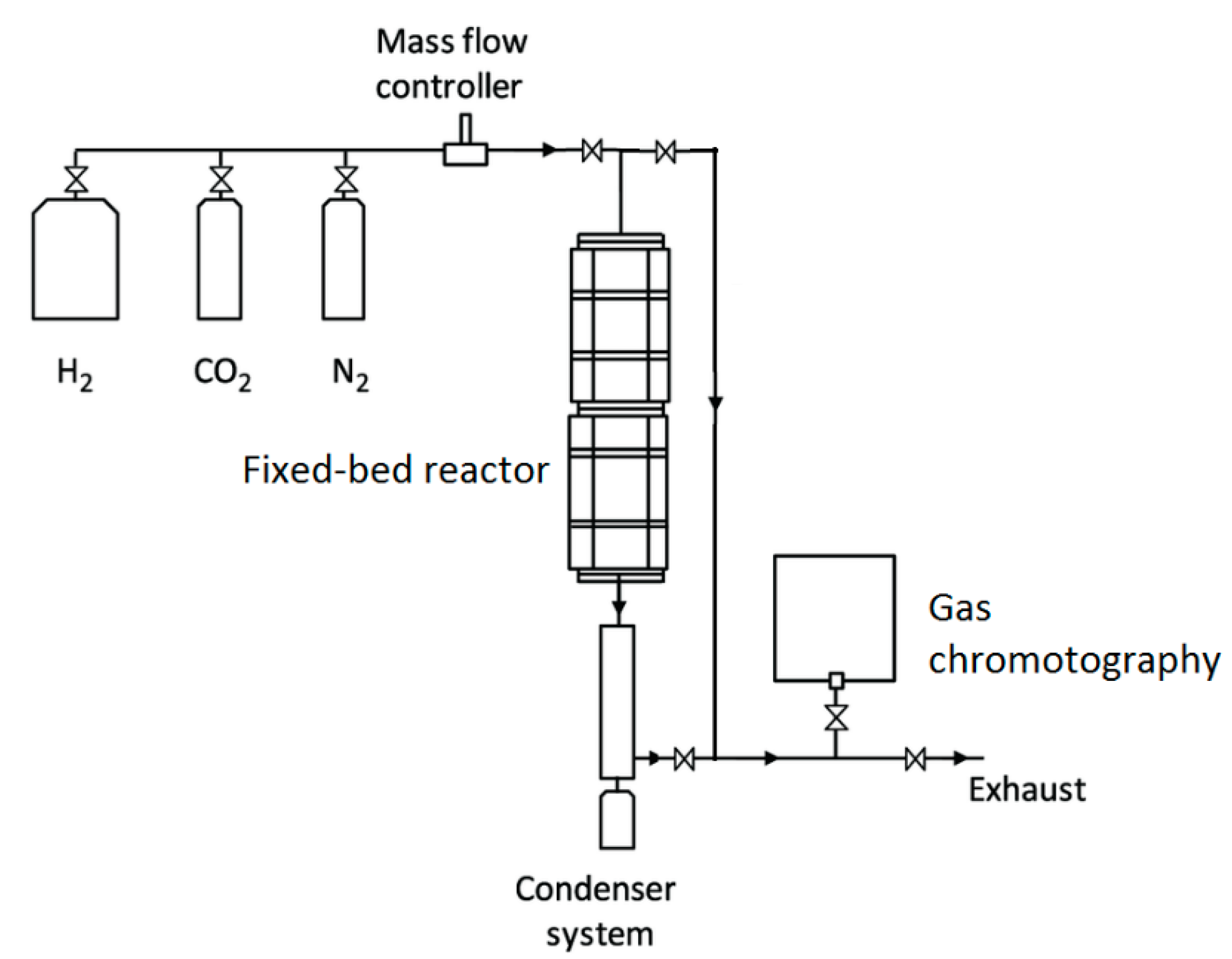
The methanation test set-up for the production of methane, a valuable product resulting from the capture and use of CO2, currently the most promising and popular technology, is shown in Figure 1. The input gases required for methane production from CO2 are CO2 and H2.
Figure 1.
Schematic diagram of the CO2 methanation process.
Figure 1.
Schematic diagram of the CO2 methanation process.
The methanation of CO
2 is an exothermic catalytic reaction and is typically operated at temperatures between 250°C and 4000°C [
12] depending on the catalyst used:
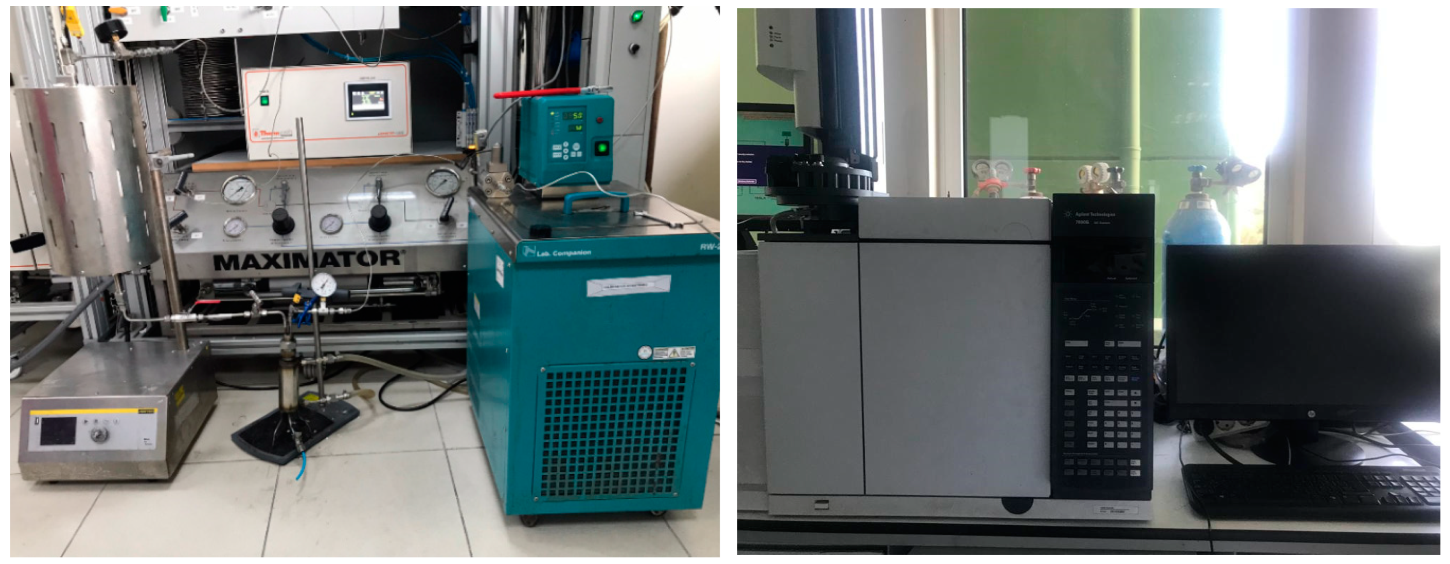
The methanation reaction was performed at experimental set-up in a fixed bed stainless steel 216 reactor with an inner diameter of 10 mm shown in Figure 2. This reactor was fixed upright inside Nabertherm NB300 furnace and a thermocouple was embedded into the center of catalyst bed to measure the temperature during the reaction.
Catalyst testing for activity were performed by using 0.5 grams of catalyst particles with 50–150 microns. Then 0.5 g of quartz particles of the same size range were added in equivalent volume to avoid localized heating. The desired gas compositions from ALICAT MFCs were adjusted and fed to the system according to the reaction conditions. Before the reaction, calcined catalysts were treated for reduction with a gas mixture composed of 10v%H
2 -90v %N
2 at 350 ⁰C for 4 h under atmospheric pressure [
13].
Figure 2.
CO2 Methanation experimental set-up.
Figure 2.
CO2 Methanation experimental set-up.
The product gas was quantitatively analyzed every 30 min by an on-line (Agilent, 7820A GC) gas chromatography equipped with a TCD detector and a Carboxen column. Methane and other hydrocarbons were detected by a flame ionization detector (FID) with Alumina S column.
Subsequently, the catalysts whose performance was measured in the GC test analysis system were tested on three different parameters. Experiments were carried out by changing the pressure, temperature and flow parameters from the reaction conditions. Conditions of 200
oC, 250
oC, 300
oC and 350
oC for temperature, 0.08, 0.16, 0.32 and 0.64 for flow and 1, 3, 5 and 10 bar for pressure were applied (
Table 1).
3. Characterization Analysis
The elementary compositions of samples were determined using a; Thermo Scientific, ARL PERFORM’X Sequential PFX-374 analyzer used as X-ray source.
A quantitative analysis of the coke amount on the used catalyst was performed with a thermogravimetry analyzer (TGA, Perkin Elmer Pyris1). Thermogravimetric analyzes are performed in a one-step temperature program. Heating is 900 oC with a heating rate of 10°C/min under 30 mL/min air flow. Approximately 10 mg of sample is used for TGA analysis.
The physical structure of the surface of catalyst was studied by scanning electron microscopy (SEM, JEOL-6390LV). The samples were coated with a Pd-Au mixture prior to analysis. SEM analysis method is an important technique for surface topography studies. In this analysis method, it provides information about the shape, size, position and morphology of metal particles on the support surface.
There are many commercially available catalysts that are utilized to produce methane from syngas. The content of one of them, was determined by XRF characterization analysis (
Table 2). As can be seen from the XRF analysis results in
Table 2, most of the commercial catalyst structure consists of nickel oxide. Apart from this, Al
2O
3, SiO
2, MgO, CuO, La
2O
3 etc. metal salts are also present in the structure.
To explore the presence of carbon deposits on the catalyst's surface, TGA and SEM analyses were performed on spent catalysts.
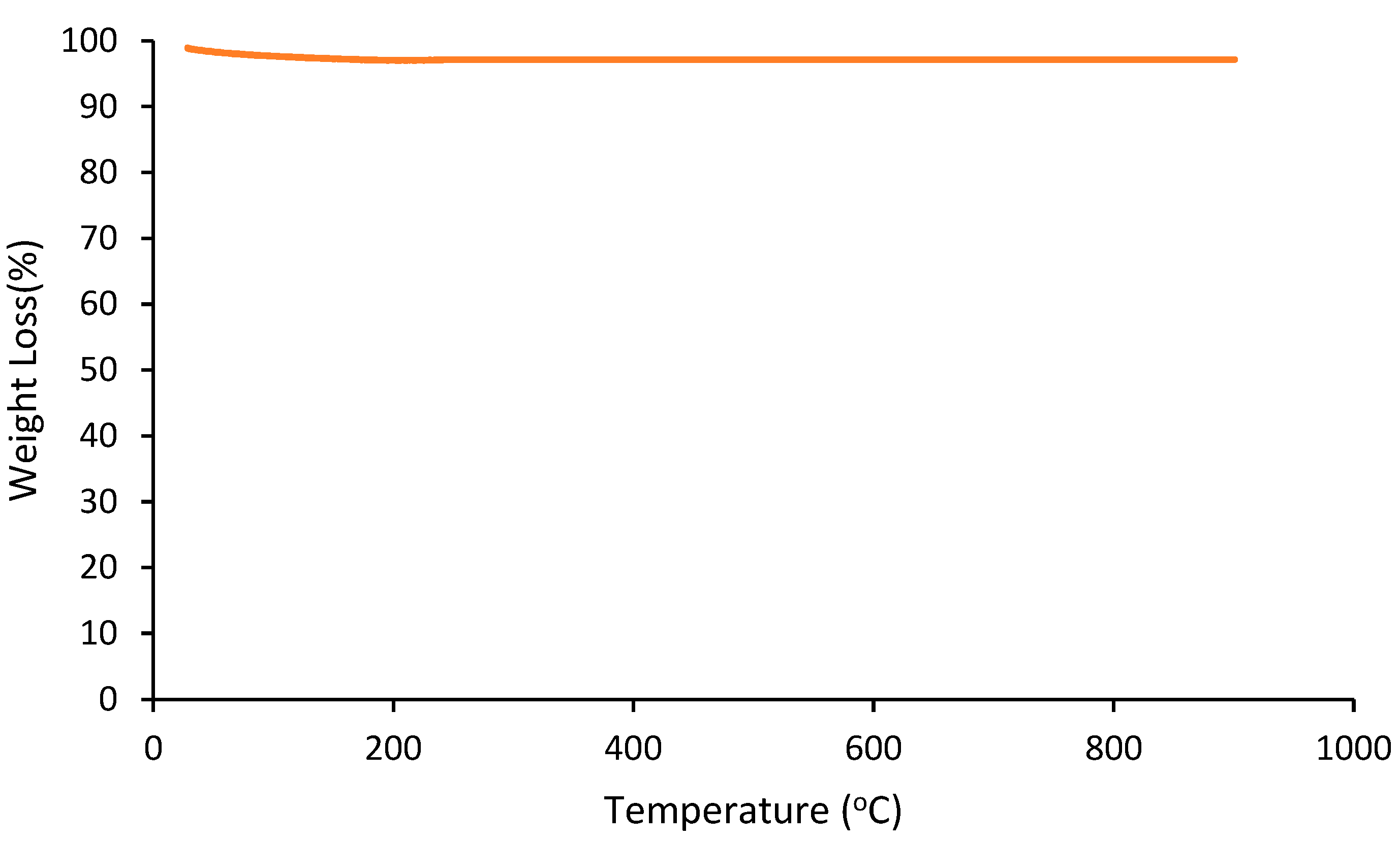
The extent of coke formation on the catalyst after the reaction was quantitatively studied by TGA in an oxidative atmosphere, and the results are shown in
Figure 1.
Figure 1 shows that there was no significant weight loss due to the C-formation. From the TGA analysis of the used catalyst, no clear evidence of carbon on the catalyst was found. This result indicates that the catalyst has the high resistance to the formation of coke.
The fresh and used catalysts were characterized with scanning electron microscopy.
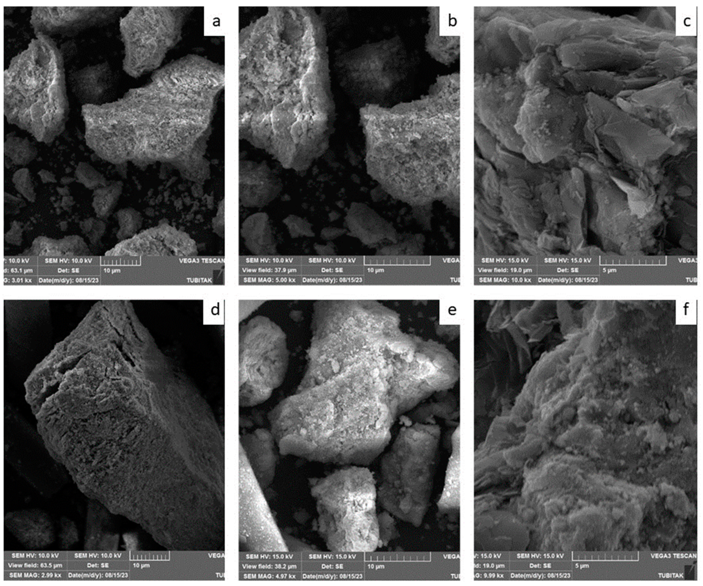
Figure 2 (a–f) illustrates the results of scanning electron microscope of the same samples. The coke formation that is expected to occur in catalysts containing Ni particles is the formation of fibrous carbon. Between the Ni particles and the support, fibrous carbon forms and grows, which leads to clogging of the catalyst pores [
14].
Figure 2 (d,e,f) SEM images show that the surface of the spent catalysts is almost smooth. The surface properties of used catalysts are very similar to those of fresh catalysts. Any fibrous structure is not observed on the surface.
Another distinctive characteristic observed in the SEM micrographs is the prevalence of bright areas is indicator of exposed nickel metal.
Figure 2, the SEM images of fresh (b) and spent (e) catalysts at the same magnification ratios show similar intensity of bright areas. This indicates that the exposed active nickel surfaces have similar amounts and are not affected by coke formation [
15].
The SEM and the TGA results confirmed each other and according to these results zero coke formation was recorded for this catalyst.
Figure 1.
Thermogravimetric profile of used catalyst.
Figure 1.
Thermogravimetric profile of used catalyst.
Figure 2.
SEM of the fresh catalyst (a) 3kx, (b) 5kx, (c)10kx. SEM of the spent catalyst (d) 3kx, (e) 5kx, (f)10kx. .
Figure 2.
SEM of the fresh catalyst (a) 3kx, (b) 5kx, (c)10kx. SEM of the spent catalyst (d) 3kx, (e) 5kx, (f)10kx. .
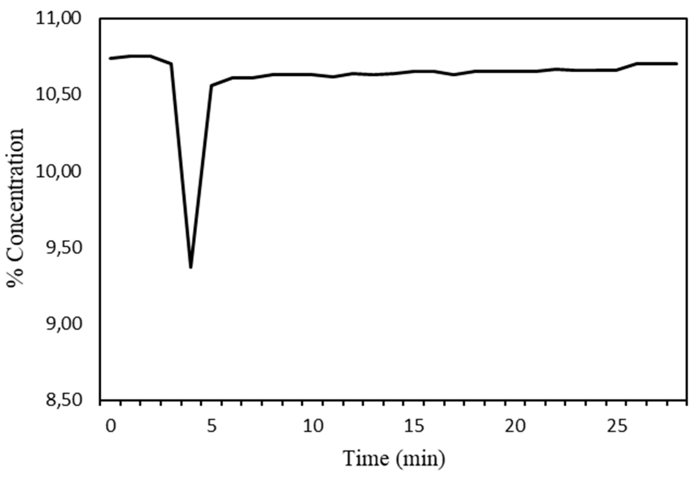
The hydrogen consumption versus time graph was generated with the data obtained (
Figure 3). It was observed that the reduction was complete.
4. Methods
4.1. Decision Tree Regression (DTR)
A decision tree is a mostly employed technique in machine learning for creating predictive models based on simple logical statements [
16]. The fundamental decision tree structure involves a starting point (root node), intermediate points (internal nodes), and end points (terminal nodes) [
17,
18]. In the context of predicting continuous variables rather than categorical ones, Decision Tree Regression (DTR) is utilized. DTR progressively divides the dataset into smaller groups to achieve better uniformity within these groups. Subsequently, it aims to minimize predictive errors within each of these divisions. This process ultimately generates predictions for continuous output variables through logical rules. In decision tree algorithms, the arrangement of these groups is determined by evaluating the information gain for all feasible groupings and selecting the grouping with the highest information gain to serve as the root node, as described in Equation (2) [
19].
In the given equation, where C represents the cluster set, A denotes the attribute, and S(C) stands for the entropy of cluster set C. The primary strength of Decision Tree Regression (DTR) over alternative modeling methods lies in its capability to generate a model that is expressed as a collection of logical rules and expressions. Moreover, it can effectively handle scenarios involving multiple output targets. Furthermore, it possesses the advantage of being easily comprehensible and interpretable, allowing for visualization of the tree structures [
20]. Notwithstanding these noteworthy qualities, decision trees come with certain drawbacks. They are not designed to accommodate outputs reliant on more than one feature, they can produce somewhat inconsistent outcomes, they exhibit high sensitivity to minor alterations in test data, and they tend to generate intricate tree configurations when dealing with numerical datasets [
17].
The evolution of utilizing decision trees in classification and estimation involves the creation of a decision tree model based on training data, the assessment of this model using test data and appropriate evaluation criteria, and the application of the resultant model to predict future values [
18].
4.2. Random Forest Regression
The method of random forest regression (RF) entails the fitting of numerous classification trees to a given dataset. Subsequently, the predictions generated by these individual trees are amalgamated to construct a final predictive model, as explained by Golden et al. in 2019 [
21]. Unlike a solitary model, the random forest approach leverages the combined predictions of multiple models to yield more robust and broadly applicable outcomes. Various ensemble techniques, including bagging and boosting, involve the utilization of multiple classifiers in a single classification task. These approaches amalgamate the outputs of these classifiers through methods such as voting or averaging to enhance predictive efficacy. Bagging, or bootstrap aggregation, is one ensemble method that entails training multiple models independently and concurrently. The resulting predictions are then combined to establish an averaged model, as elaborated by Soni et al. in 2021 [
22]. Boosting, on the other hand, is a distinct ensemble method involving the sequential and adaptive training of weak learners to enhance the predictions of a learning algorithm. Within the context of the RF method discussed in this study, the least-squares boosting algorithm was employed. This algorithm involves fitting the residual errors of individual weak learners to achieve superior performance.
4.3. Gaussian Process Regression
GPR represents a machine learning technique. This specific algorithm is kernel-centered, not relying on fixed parameters, and has a foundation in probability [
23]. Regression models utilizing Gaussian processes are entirely rooted in probability, adaptable, and straightforward to employ, leading to their widespread use across various applications. However, its drawback lies in its effectiveness being constrained to a relatively small number of cases, usually no more than a few thousand. This limitation stems from the rapid increase in computational and memory demands, growing cubically and quadratically with the number of training cases, respectively [
24].
A Gaussian process is fully defined by its mean function, denoted as m(x), and covariance function, represented as k(x, x'). These functions describe a real process f(x), as shown in Equation (3) [
25,
26]. When appropriately scaled, the mean function m(x) can often be set to zero [
25,
27].
An algorithm for application of GPR is as follows [
25]:
Input: X (inputs), y (targets), σ2 (noise level), x* (test input).
α : = LT\(L\y)
: = α
8. Return:
(log marginal likelihood)
4.4. Support Vector Machines
Support Vector Machines (SVM) have gained popularity in the realm of machine learning due to their non-parametric structure and incorporation of kernel functions. Among SVM techniques, SVM stands out as a method tailored for predicting continuous variables. Differing from polynomial regression and Artificial Neural Networks (ANNs), SVM models are trained by minimizing the bound on generalization error, as opposed to prediction error [
28]. Thus, SVM models prioritize achieving optimal generalization performance.
The fundamental principle of SVM involves mapping data to a higher-dimensional feature space using a kernel function. Within this space, an optimal hyperplane is sought, aiming to minimize a chosen cost function [
29]. Consequently, SVM conducts linear regression within an expanded dimensionality using a kernel function (denoted as K) as depicted in Equation (4).
In contrast, ANNs possess a distinctive capability to predict multiple output variables using a single model. In the context of this study, where the dataset contains four features and four corresponding output variables, a singular ANN model was devised. This model comprises two hidden layers, each containing nine neurons, as illustrated in
Figure 1. The hidden layers employ sigmoid activation functions, while the output layer employs a linear activation function. The training of the neural network involves adjusting connection weights to minimize the disparity between predictions and actual outputs, with the widely used backpropagation algorithm employed for this purpose [
30].
In the given context, the symbols 𝛽𝑖 and 𝑐 represent constant coefficients, while ( , 𝑥) stands for the kernel function. Within this study, a kernel function in the form of a second-degree polynomial (as indicated by Equation 5) was employed. This specific kernel was chosen due to the limitations observed with linear and Gaussian kernels in capturing the intricacies of the problem at hand. Both linear and Gaussian kernels exhibited insufficient predictive capabilities, prompting the exploration of alternative kernels.
While the use of third-degree or higher polynomial kernels could potentially enhance performance, their adoption was deemed impractical due to substantial computational overhead. The marginal performance gain achieved by these higher-degree kernels did not justify the extensive training time they demanded.
Throughout the training phase of the models, the epsilon-insensitive cost function (expressed through Equations 6 and 7) was utilized and subsequently minimized.
4.5. Validation Method: K-fold Cross Validation (KCV)
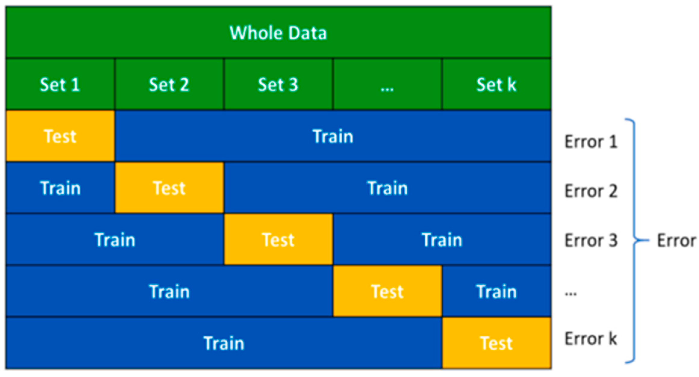
Cross-validation methods are used to objectively evaluate the performance of a prediction model. K-fold cross-validation (KCV) is a highly preferred cross-validation technique due to its use of the entire data set [
31]. In KCV, the data is divided into k equally sized partitions (folds). The candidate model is then trained on training folds and evaluated on the remaining test fold [
32]. This process is repeated k times with a different fold as the test set each time, ensuring that all data is used for both training and testing. In this study, 'K' is chosen as ten because it has been shown to reflect the most unbiased generalization performance of the models compared to other choices. This approach reduces variance by using 10 different partitions, and the performance estimate is less sensitive to the random partitioning of the data compared to other cross-validation methods [
33].
Figure 4.
The principles of k-fold cross validation.
Figure 4.
The principles of k-fold cross validation.
5. Results & Discussion
All prediction models are trained to predict CO
2 methanation output concentrations and their performances are evaluated according to their test performance in 10-fold cross validation technique. R-squared (R²) is a statistical measure that represents the proportion of variance in the dependent variable (outcome) that's explained by the independent variables (predictors) in a regression model. It is also called the coefficient of determination. R-squared is used to assess the goodness of fit of a regression model and how well the model's predictions match the actual observed data. Adjusted R
2 shows how well the terms fit a line, but adjusts for the number of terms in a pattern. Root mean square error (RMSE) measures the average difference between a statistical model's predicted values and the actual values. Normalized Root Mean Square Error (NRMSE) calculates relative error between predicted and observed values [
34]. Absolute Average Error (AAE) is a measure of the average size of the mistakes in a collection of predictions, without taking their direction into account.
When analyzing the data in
Table 3, the R
2 value indicating linearity is expected to be closest to 1 and the RMSE value indicating the error rate is expected to be the smallest. Looking at
Table 3, it is seen that the RF method is the closest to 1 with an R
2 value of 0.987 for CO
2 data. This is supported by the smallest RMSE value of 0.526. The RF method was determined to be the most appropriate method for CO
2 conversion data. When the H
2 conversion data is analyzed, it is seen that the RF method has the closest R
2 value to 1 with 0.987. Although the error rate of 2.292 is very large, it is the smallest among the RMSE values and the most appropriate method is determined as RF method. In N
2 data, the closest R
2 value to 1 is seen in the DT method with 0.986. The smallest RME value is 1.392, supporting the selection of DT as the most appropriate method. In the CH
4 data, the largest R
2 value is seen in the DT method and this is supported by the RMSE value of 1.640. As a result, RF method selection in CO
2 and H
2 data, DT method selection was determined as the most suitable for processing N
2 and CH
4 data.
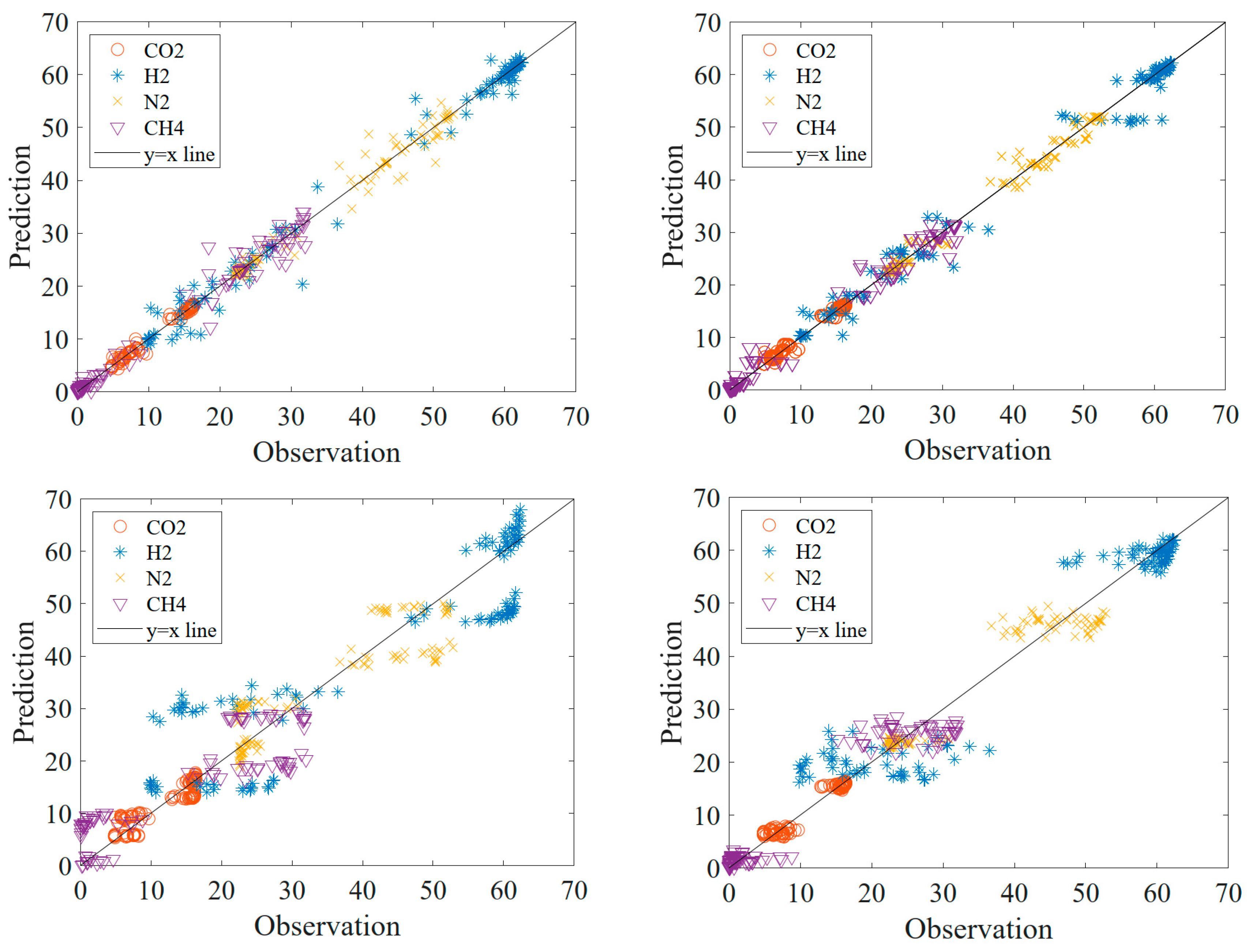
When
Figure 5 is analyzed, it is seen that the data in SVM and GO methods are too much out of the line. The data outside the line are more than the data in RF and DT methods. It is also seen that there is clustering in the data in DT, SVM and GP methods. This proves that these models are more inappropriate than RF. For these reasons, it is decided that RF is the most appropriate model.
When
Table 4 is examined, R
2 values close to 1 are important for the accuracy of the data. In the 4th research article, it is seen that the train R
2 value is smaller than the test R
2 value. This situation is far from reality. Although there is a lot of data in research articles 1 and 7, it is seen that the R
2 values of the tests are far from 1. In research paper 10, the number of data is close to the number of data in this study, but it is seen that it does not reach the R
2 value we have reached. Among the R
2 values in the literature studies, this study has the closest R
2 value to 1. It is seen that the best result among the literature studies is reached in this study.
6. Conclusions
SEM and TGA techniques were used to both qualitatively and quantitatively analyze the presence of carbon deposition. From the TGA graph the spent catalyst displayed no weight loss in the spent catalyst, indicating an absence of coke. TGA and SEM results confirmed each other and according to these results zero coke formation was recorded for this catalyst.
The RF method was the most successful method with an R2 value of 0.987 for CO2 data. The method was also successful to predict other gas concentrations. The results were compared with the literature. It is seen that the best result among the literature studies is reached in this study. With this study, we show that the use of machine learning methods is capable of predicting output concentration of CO2 methanation process. The RF methods have a low computational requirement to make predictions once it is trained. Therefore, this study offers more flexibility in controlling and optimizing conversion of CO2.
References
- Yılmaz, B., Oral, B., & Yıldırım, R. (2023). Machine learning analysis of catalytic CO2 methanation. International Journal of Hydrogen Energy, 48(64), 24904-24914. [CrossRef]
- Hong, T., Saifuddin, N., Halim, S., Young-Kwon, P., Hernández, & H., Loke, S. (2022). “Current Developments in Catalytic Methanation of Carbon Dioxide—A Review” Frontiers in Energy Research Vol. 9 https://10.3389/fenrg.2021.795423.
- Kim, C., Yoo, C., Oh, H., Min, B., & Lee, U. (2022). “Review of carbon dioxide utilization technologies and their potential for industrial application”, Journal of CO2 Utilization, Volume 65. [CrossRef]
- Dashti, A., Bazdar, M., Fakhrabadi, E., & Mohammadi, A. (2022). Modeling of Catalytic CO2 Methanation Using Smart Computational Schemes. Chemical Engineering & Technology, 45, 135-143. [CrossRef]
- Fedorov, A., & Linke, D. (2022). Data analysis of CO2 hydrogenation catalysts for hydrocarbon production. Journal of CO2 Utilization, 61. [CrossRef]
- Ngo, S. I., & Lim, Y.-I. (2021). Solution and Parameter Identification of a Fixed-Bed Reactor Model for Catalytic CO2 Methanation Using Physics-Informed Neural Networks. Catalysts, 11(11), 1304. [CrossRef]
- Suvarna, M., Araújo, T. P., & Pérez-Ramírez, J. (2022). A generalized machine learning framework to predict the space-time yield of methanol from thermocatalytic CO2 hydrogenation. Applied Catalysis B: Environmental, 315. [CrossRef]
- Chattoraj, J., Hamadicharef, B., Kong, J., Pargi, M. K., Zeng, Y., Poh, C. K., Chen, L., Gao, F., & Tan, T. L. (2022). Theory-Guided Machine Learning to Predict the Performance of Noble Metal Catalysts in the Water-Gas Shift Reaction. ChemCatChem, 14. [CrossRef]
- Pérez, S., Aragón, J. J., Peciña, I., et al. (2019). Enhanced CO2 Methanation by New Microstructured Reactor Concept and Design. Topics in Catalysis, 62, 518–523. [CrossRef]
- Shen, Y., Dong, Y., Han, X., Wu, J., Xue, K., Jin, M., Xie, G., & Xu, X. (2023). Prediction model for methanation reaction conditions based on a state transition simulated annealing algorithm optimized extreme learning machine. International Journal of Hydrogen Energy, 48, 24560-24573. [CrossRef]
- Praveen, C. S., & Comas-Vives, A. (2020). Design of an Accurate Machine Learning Algorithm to Predict the Binding Energies of Several Adsorbates on Multiple Sites of Metal Surfaces. ChemCatChem, 12. [CrossRef]
- Yeo, C.-E., Seo, M., Kim, D., Jeong, C., Shin, H.-S., & Kim, S. (2021). Optimization of Operating Conditions for CO2 Methanation Process Using Design of Experiments. Energies, 14(24), 8414. [CrossRef]
- Kristiani, A., & Takeishi, K. (2022). CO2 methanation over nickel-based catalyst supported on yttria-stabilized zirconia. Catalysis Communications, 165. [CrossRef]
- Song, D. H., Jung, U. H., Kim, Y. E., Im, H. B., Lee, T. H., Lee, K. B., & Koo, K. Y. (2022). Influence of Supports on the Catalytic Activity and Coke Resistance of Ni Catalyst in Dry Reforming of Methane. Catalysts, 12(2). [CrossRef]
- Venugopal, A., Naveen Kumar, S., Ashok, J., Hari Prasad, D., Durga Kumari, V., Prasad, K. B. S., & Subrahmanyam, M. (2007). Hydrogen production by catalytic decomposition of methane over Ni / SiO2. International Journal of Hydrogen Energy, 32(12), 1782–1788. [CrossRef]
- Özkan, K., Işık, Ş., Günkaya, Z., Özkan, A., & Banar, M. (2019). A heating value estimation of refuse derived fuel using the genetic programming model. Waste Management, 100, 327-335. [CrossRef]
- Rokach, L., & Maimon, O. (2010). Classification Trees. In O. Maimon & L. Rokach (Eds.), Data Mining and Knowledge Discovery Handbook (pp. 149-174). Springer US. [CrossRef]
- Zhao, Y., & Zhang, Y. (2008). Comparison of decision tree methods for finding active objects. Advances in Space Research, 41, 1955-1959. [CrossRef]
- Quinlan, J. R. (1986). Induction of decision trees. Machine Learning, 1, 81-106. [CrossRef]
- Elmaz, F., Yücel, Ö., & Mutlu, A. Y. (2020). Machine learning based approach for predicting of higher heating values of solid fuels using proximity and ultimate analysis. International Journal of Advances in Engineering and Pure Sciences, 32(2), 145-151. [CrossRef]
- Golden, C. E., Rothrock, M. J., Jr., & Mishra, A. (2019). Comparison between random forest and gradient boosting machine methods for predicting Listeria spp. prevalence in the environment of pastured poultry farms. Food Research International, 122, 47-55. [CrossRef]
- Soni, A., Al-Sarayreh, M., Reis, M. M., & Brightwell, G. (2021). Hyperspectral imaging and deep learning for quantification of Clostridium sporogenes spores in food products using 1D-convolutional neural networks and random forest model. Food Research International. [CrossRef]
- Makridakis, S., Spiliotis, E., Assimakopoulos, V., & Hernandez Montoya, A. R. (2018). Statistical and Machine Learning forecasting methods: Concerns and ways forward. PLoS One, 13(3), e0194889. [CrossRef]
- Candela, J. Q., & Rasmussen, C. (2005). A Unifying View of Sparse Approximate Gaussian Process Regression. Journal of Machine Learning Research, 6, 1939-1959.
- Rasmussen, C. E., & Williams, C. K. I. (2006). Gaussian Processes for Machine Learning. Massachusetts Institute of Technology.
- Mathworks. (2021). Gaussian Process Regression Models. https://www.mathworks.com/help/stats/gaussian-process-regression-models.html.
- Birgen, C., Magnanelli, E., Carlsson, P., Skreiberg, Ø., Mosby, J., & Becidan, M. (2021). Machine learning based modelling for lower heating value prediction of municipal solid waste. Fuel, 283, 118906. [CrossRef]
- Evgeniou, T., Pontil, M., & Poggio, T. (2000). Regularization Networks and Support Vector Machines. Advances in Computational Mathematics, 13(1), 1-50. [CrossRef]
- Hecht-Nielsen, R. (1988). Theory of the backpropagation neural network. Neural Networks, 1(1), 445. [CrossRef]
- Smola, A. J., & Schölkopf, B. (2004). A tutorial on support vector regression. Statistics and Computing, 14(3), 199-222. [CrossRef]
- Elmaz, F., Yücel, Ö., & Mutlu, A. Y. (2019). Evaluating the effect of blending ratio on the co-gasification of high ash coal and biomass in a fluidized bed gasifier using machine learning. Mugla Journal of Science and Technology, 5(1), 1-12. [CrossRef]
- Büyükçakir B, Mutlu AY. Comparison of hilbert vibration decomposition with empirical mode decomposition for classifying epileptic seizures. In: 2018 52nd asilomar conference on signals, systems, and computers. IEEE; 2018. p. 357e62.
- Ambroise C, McLachlan GJ. Selection bias in gene extraction on the basis of microarray gene-expression data. Proc Natl Acad Sci 2002;99(10):6562e6. [CrossRef]
- Yaka, H., Insel, M. A., Yucel, O., & Sadikoglu, H. (2022). A comparison of machine learning algorithms for estimation of higher heating values of biomass and fossil fuels from ultimate analysis. Fuel, 320, 123971. [CrossRef]
|
Disclaimer/Publisher’s Note: The statements, opinions and data contained in all publications are solely those of the individual author(s) and contributor(s) and not of MDPI and/or the editor(s). MDPI and/or the editor(s) disclaim responsibility for any injury to people or property resulting from any ideas, methods, instructions or products referred to in the content. |
© 2023 by the authors. Licensee MDPI, Basel, Switzerland. This article is an open access article distributed under the terms and conditions of the Creative Commons Attribution (CC BY) license (http://creativecommons.org/licenses/by/4.0/).
