Application of Machine Learning to Estimate Ammonia Atmospheric Emissions

Ammonia is an atmospheric pollutant, predominantly emitted from agriculture, leading acidification and eutrophication of soil and water and contributing to secondary PM2.5. The implementation of accurate emission inventories with high spatial and time resolution plays a fundamental role in the development of air modelling simulation and in the impact assessment of actions for air quality improvement. The development and release of new algorithms and the increase of data availability are supporting the implementation of machine learning approaches in environmental and air quality data analysis. In this paper we present a methodology developed by the application of the Random Forest algorithm to bottom-up local emission inventories of ammonia to validate annual time series of ammonia emissions and calculate high resolution temporal profiles. The model has been trained and tested by the hourly measurements of ammonia concentrations and atmospheric turbulence parameters starting from a constant emission scenario. The initial values of emissions are calculated based on a bottom-up emission inventory detailed at the municipal basis and considering a circular area of about 4 km radius centered on measurement sites. By comparing predicted and measured concentrations, the emissions are modified, the model's training and testing are repeated, and the model converges to a very high performance in predicting ammonia concentrations and establishing an hourly time changing emission profile. The site-specific emissions profiles, estimated by the proposed methodology, clearly show a nonlinear relation with measured concentrations and allow to identify the effect of atmospheric turbulence on pollutant accumulation. The estimated time series well confirm the available data of the emission inventories and the monthly emission profiles have been compared with estimated data from satellite.

Keywords:

Subject: Environmental and Earth Sciences - Pollution

1. Introduction

Primary atmospheric emissions of ammonia (NH₃) can react with nitrogen and sulfur oxides contributing significantly to the formation of secondary inorganic PM_2.5 and lead to acidification and eutrophication of soil and water [1]. The importance of monitoring atmospheric ammonia is well recognized, defining ammonia as one of the most crucial substances to monitor among greenhouse gases and particulate matter [2,3,4,5]. International and National regulations on air pollution require reduction of atmospheric emissions of ammonia as for nitrogen oxides (NO_x), non-methane volatile organic compounds (NMVOCs), sulfur dioxide (SO₂), and fine particulate matter (PM_2.5) [6,7,8]. Emission inventories play a fundamental role in the estimation of emission reduction, their accuracy is determinant in supporting Air Quality Plans and policy makers [9,10].

In Europe the agriculture sector contributes around 94% of total ammonia emissions [11] and this data is confirmed in Italy [12] and in the Po-basin area 97% [13]. The Po-basin is the highest populated area of Italy. Placed in the north of the country, it is surrounded by mountains and often suffers from atmospheric stagnation and thermal inversion conditions. In the Po-basin, areas with high population density are interspersed with intensive farming areas. According to the national veterinary records office [14], about 80% of cows, swine and poultry are bred in the regions of the Po-basin, determining relative higher emission density of ammonia compared to Italy and EU-27 [13]. In northern Italy, livestock contributes around 83% of the total ammonia emissions and the use of mineral fertilizers contributes for 15%. NH₃ from livestock are occurring during animal housing, manure storage, spreading and grazing, this latter phase is relatively negligible, considering the intensive level of farming in Northen Italy.

In national and local emission inventories, the estimates of total annual ammonia emission are based on animal numbers, fertilizers consumptions and emission factors. Emission factors aim to describe how nitrogen (N) in manure and in fertilizers is lost as ammonia in the atmosphere.

In livestock the efficiency of conversion of N content in the animal food influences the nitrogen content in the manure and the amount of ammonia potentially emitted.

The rate of ammonia emission from manure exposed to ambient air is influenced by several factors. These include the concentration of ammoniacal components in the manure, the concentration of NH₃ at the exchanging surface and in the atmosphere above the manure, and air turbulence conditions. The temperature and pH of the manure can affect the NH₃ concentration at the exchanging surface, while meteorological factors can influence the turbulence around the emitting sources [15]. Emissions occur primarily after and not during spreading [15] and are also influenced by viscosity, dry matter content of manure applied on land surface.

Emissions are also influenced by the application technique, which affects the real exchanging surface of ammonia emissions. The level of atmospheric turbulence and the concentration of ammonia at the interface exchange may also impact emissions from synthetic fertilizers. Chemical composition of fertilizers affects the interphase ammonia concentration [16].

In atmosphere ammonia can react with acid gases, sulphuric, nitric and hydrochloric acids, with reaction rates depending on concentrations, temperatures and humidity [15]. These reactions play a fundamental role in the formation of secondary aerosols and in the dry and wet deposition of ammoniacal substances because gaseous ammonia is commonly dry deposited at a high rate, while ammoniacal substances are deposited slowly. The contribution of NH₃ emissions to the formation of secondary particulate matter is highlighted for the Po-basin by different studies [17,18]. As a matter of facts, atmospheric turbulence seems affecting in more than one way the release of ammonia. The time modulation of ammonia emissions in a chemistry transport model (CTM) can be estimated based on time varying meteorological variables, as reported by different research [1,19,20,21,22,23,24]. As evidenced by previous studies, emission time profiles rather defined on meteorological variables strongly affect the atmospheric concentrations of NH₃ [1,19,20,21,22,23,24,25].

The above-mentioned variables are used to fit several detailed models [26,27,28,29,30,31,32] and the use of machine learning approach has been investigated for estimating time varying ammonia emission [2,33,34,35]. As reported by Hempel et al. [2], the development and release of new algorithms and the increase of data availability support the implementation of machine learning approaches also in different sectors of agriculture [36].

The main goal of this research is to implement a machine learning approach capable of achieving several objectives. These include: 1) predicting the hourly site-measured ammonia concentration in different site areas in northern Italy, 2) calculating the hourly varying emissions for each measurement site, 3) validating the annual emission estimates of the emission inventory, and 4) defining and comparing also with satellite data the time-varying monthly ammonia emission profiles for different sites.

The implemented approach is based on several key assumptions. Firstly, an area with a radius of 3.6 km is considered for each measurement site, due to the maximum distance of air with a wind velocity of 1 m/s, which is typical for the region. Secondly, a Random Forest model is trained and tested on the measured hourly ammonia concentrations, using measured turbulence parameters and a first guess of the total emission of NH₃ as input variables. The first guess emission value is defined from the local emission inventory, considering an average local value within the circled area around the site. Finally, the test and training of the Random Forest model is reiterated, correcting the hourly emissions by the ratio between measured and estimated concentrations.

2. Materials and Methods

This section describes the data that were used and the description of the calculation model implemented in this study.

2.1. Measurements sites and data

An extremely large dataset for ten measurements sites located in the Lombardy region, in northern Italy is analyzed, including:

hourly measured ammonia concentrations
hourly based meteorological variables
ammonia emission estimates

The collected dataset covers a nine-year period (start of 2014 - end of 2022), except for the location of Moggio (7_RB). Where the time series is from 2014 to the beginning of 2021 due to lack of data.

Table 1 presents the identification codes for the different measurement sites, along with the average values of ammonia concentration and wind speed measured for the entire dataset. For each site, the table also reports the emission estimates for the surrounding area of the measurement station for the years 2014, 2017, and 2019.

2.1.1. Ammonia Measurements Sites

The ammonia measurements sites considered in this study belong to the Air Quality Monitoring Network of Lombardy. The stations differ according to the type, including rural background (RB) (i.e. Bertonico, Corte de Cortesi, Cremona via Gerre Borghi and Schivenoglia), urban background (UB) (i.e. Cremona via Fatebenefratelli, Milano Pascal Città Studi and Pavia via Folperti), suburban background (SU) (i.e. Colico) and urban industrial (UI) (Sannazzaro de’ Burgondi) and to the altitude, ranging from 16 m asl (i.e. 10_RB, Schivenoglia) to 1197 m asl (i.e. 7_RB, Moggio).

2.1.2. Meteorological Parameters Measurements Sites

In this study, several meteorological variables are considered that could potentially affect the accumulation processes of ammonia in the atmosphere. These variables include wind direction (°), precipitation (mm), global solar radiation (W/m²), ambient temperature (°C), relative humidity (%), and wind velocity (m/s). These data are obtained from the monitoring network of ARPA Lombardia.

Since not all the ammonia monitoring sites were completely equipped with sensors for recording the meteorological parameters, it has been necessary to consider those from the closest meteorological station/stations if meteorological data were not available.

Therefore, for the locations of Bertonico (1_RB), Cremona Via Fatebenefratelli (4_UB), Cremona Via Gerre Borghi (5_RB) and Pavia Via Folperti (8_UB), fully equipped, meteorological data were downloaded together with ammonia concentrations data. On the other hand, for the locations of Colico (2_SU), Corte de Cortesi (3_RB), Milano Pascal Città Studi (6_UB), Moggio (7_RB), Sannazzaro (9_UI) and Schivenoglia (10_RB), it was necessary to integrate the missing data from the nearest meteorological station/stations.

2.1.3. Annual emission estimates

Emissions annual estimates in the surrounding NH₃ measurement sites are referring to 2013, 2017 and 2019 years and are obtained from the common air emission datasets developed by ARPA Lombardia in the frame of the “LIFE PREPAIR inventory” (LPi) [13]. Since no emission assessment is available for 2014, the year of the beginning of the time series considered in this study, the closest data from the inventory edition for 2013 were used for this year.

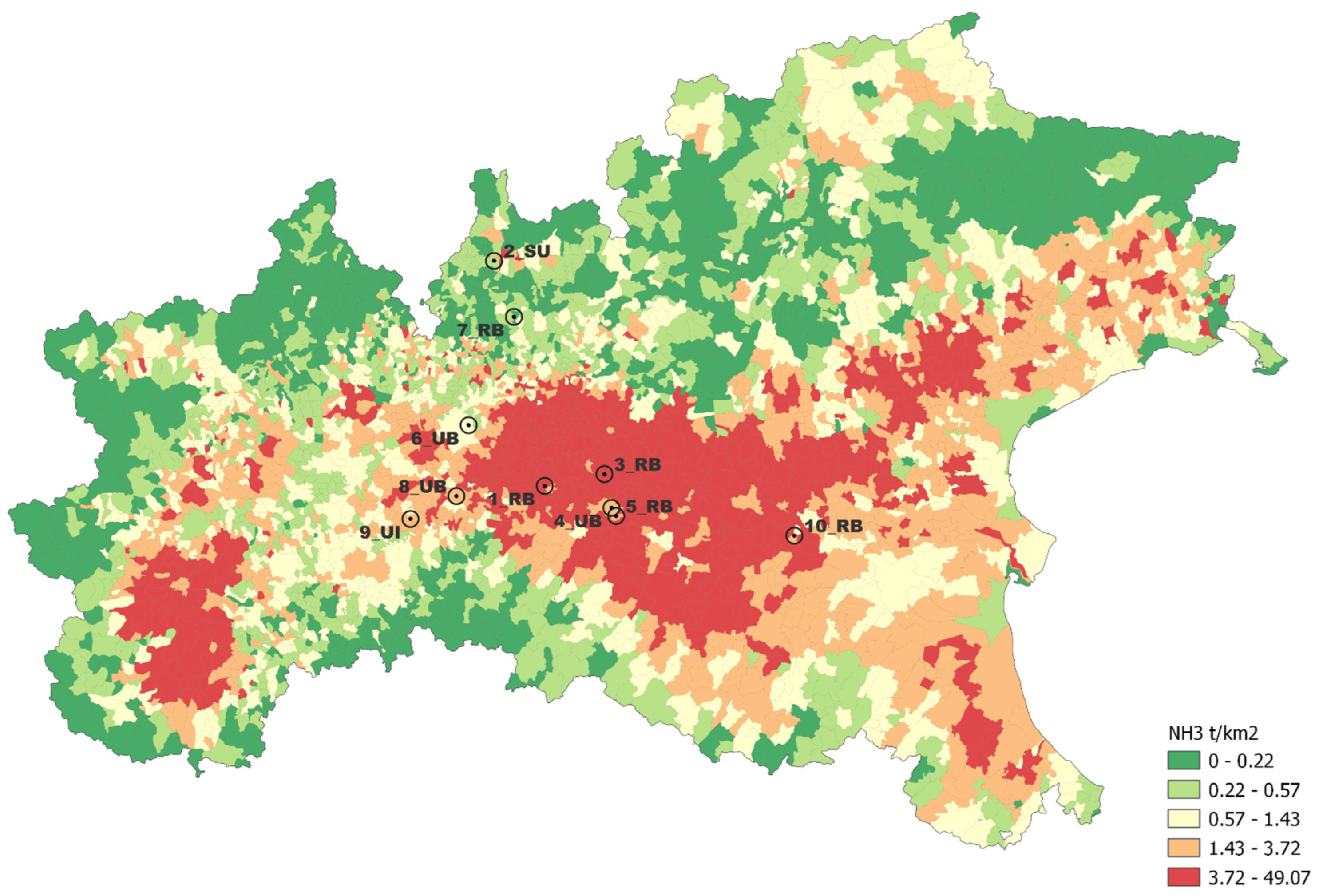
The work of updating of Po-basin inventories with a high spatial resolution scale at the municipal level was carried out by environmental protection agencies and the regions of Lombardy, Emilia-Romagna, Piedmont, Veneto, Friuli Venezia Giulia, Valle d'Aosta, Bolzano and the province of Trento. Figure 1 shows the emission density map of NH₃ of LPi referred to 2017 and the position of the ten measurements sites of ammonia.

NH₃ emission sources in LPi are described according to the SNAP classification where several categories may be identified as: fertilizer application, livestock, traffic, residential/commercial, industry and other; and several subcategories identified as: animal subcategories, vehicles subcategories, domestic combustion, agricultural soils, etc.

In the present study and in Table 1, the ammonia sources of interest are grouped into three categories: “agriculture”, “road transport” and “other sources”. In other sources are accounted minor contributes to ammonia emissions from: other sources and absorptions, non-industrial combustion and waste treatment and disposal and energy production and fuel transformation.

The LPi is obtained by multiplying the activity levels by the corresponding emission factors and aggregating the values of all municipalities, all sources and all fuel types during a full year. The specific equation is reported in the following:

E_{m} = \sum_{s}^{} \sum_{f}^{} I_{s, f, m} \times {E F}_{s, f}

(1)

where:

E_m = NH₃ annual emission for the municipality

s = source type

f = fuel type

I_s,f,m = activity indicator

EF_s,f = NH₃ emission factor

The compilation of inventories on a municipal scale was effective and comparable despite the many subjects involved thanks to the use of the same "INEMAR database" modeling system which follows the guidelines of the EEA [9,10].

An estimation of emissions is possible thanks to high-resolution maps from the LPi. A circle with a radius of 3.6 km is set around the measuring station and the quantity of ammonia emitted relative to that area is extracted. This distance was chosen because NH₃ concentrations decrease rapidly within the first 1-2 km from the sources [15]. By intersecting the map of LPi municipal areas with the circle area, it is possible to calculate the portion of the municipal area reported that is located within the area of the measuring station. The total emission for each station (𝐸_m) is given by the sum of the LPi emissions of individual municipalities calculated in proportion to how much of their territorial area falls within the area around the measuring station:

E_{s} = \sum_{m = 1, 2 . .}^{n} \frac{E_{m} \times A_{C ⋂ m}}{A_{m}}

(2)

where:

E_{s}

= emission station

E_{m}

= total municipal NH₃ emission

A_{m}

= total municipal area

A_{C ⋂ m}

= municipal area within circle area station

The overall dataset examined in the present study is characterized, with respect to previous experiences of data collection Agrimonia [37], for the use of the bottom up LPi, together with the hourly data of ammonia concentrations and the main meteorological parameters on long-term time series.

2.2.1. Machine Learning Method and Random Forest

The entire dataset encompasses 626646 valid hourly observations of ammonia concentrations and atmospheric turbulence parameters. The correlation parameters have been calculated both on the entire dataset and considering each site separately. This analysis has been extended considering different quartiles both on single stations and the entire dataset, table S1 in supplementary materials. The correlation analysis does not reveal any important correlation between concentrations and atmospheric turbulence indicators. This suggests the implementation of more sophisticated machine learning approach.

Hempel et al. have recently investigated how the selection of training data and modelling approach affects the estimation of ammonia emissions from a naturally ventilated dairy barn [2]. In their work, they concluded that ensemble methods of gradient boosting and random forest gave the best predictions for the emissions confirming that machine learning approaches can improve emissions predictions.

This study is based on the random forest method: randomForestSRC [38,39,40], implemented in a CRAN compliant R-package [41] using fast OpenMP parallel processing to construct forests for regression, classification, survival analysis, competing risks, multivariate, unsupervised, quantile regression and class imbalanced q-classification [41]. The methodology implements Breiman random forests [42] in a variety of problems.

The approach called Random Forests (RF) can improve ensemble learning by injecting randomization into the base learning process [42]. In RF the predictions are obtained by means of the trees on features subsets [43]. This approach has been extended in Random Survival Forest (RSF) developed by Ishwaran et al. [40,41,42,43,44]. RF is a method that averages trees and develops the ensemble by a randomization in the learning process in two ways: random sample of the data to grow a tree and random feature selection.

2.2.2. Sampling of Training Data and Cross-Validation

The hourly emission flux of ammonia F_NH₃ [kg/h] must be considered as an input variable of the machine learning model together with atmospheric turbulence parameters. The RandomForest is applied simulating each measuring site as reported in Figure 1, considering measured hourly values of: NH₃ concentration, temperature, precipitation, wind intensity and direction, solar radiation, humidity and first guess hourly ammonia emissions. The first guess value for ammonia emission flux is calculated for each site from LPi for 2017 as a reported in table 1. The dataset is filtered omitting missing values and according to NH₃ concentration less than 0.99 percentile. For the training and test the dataset is randomly divided into two subsets: one containing 70% of the data for training and the other with 30% of data for the test.

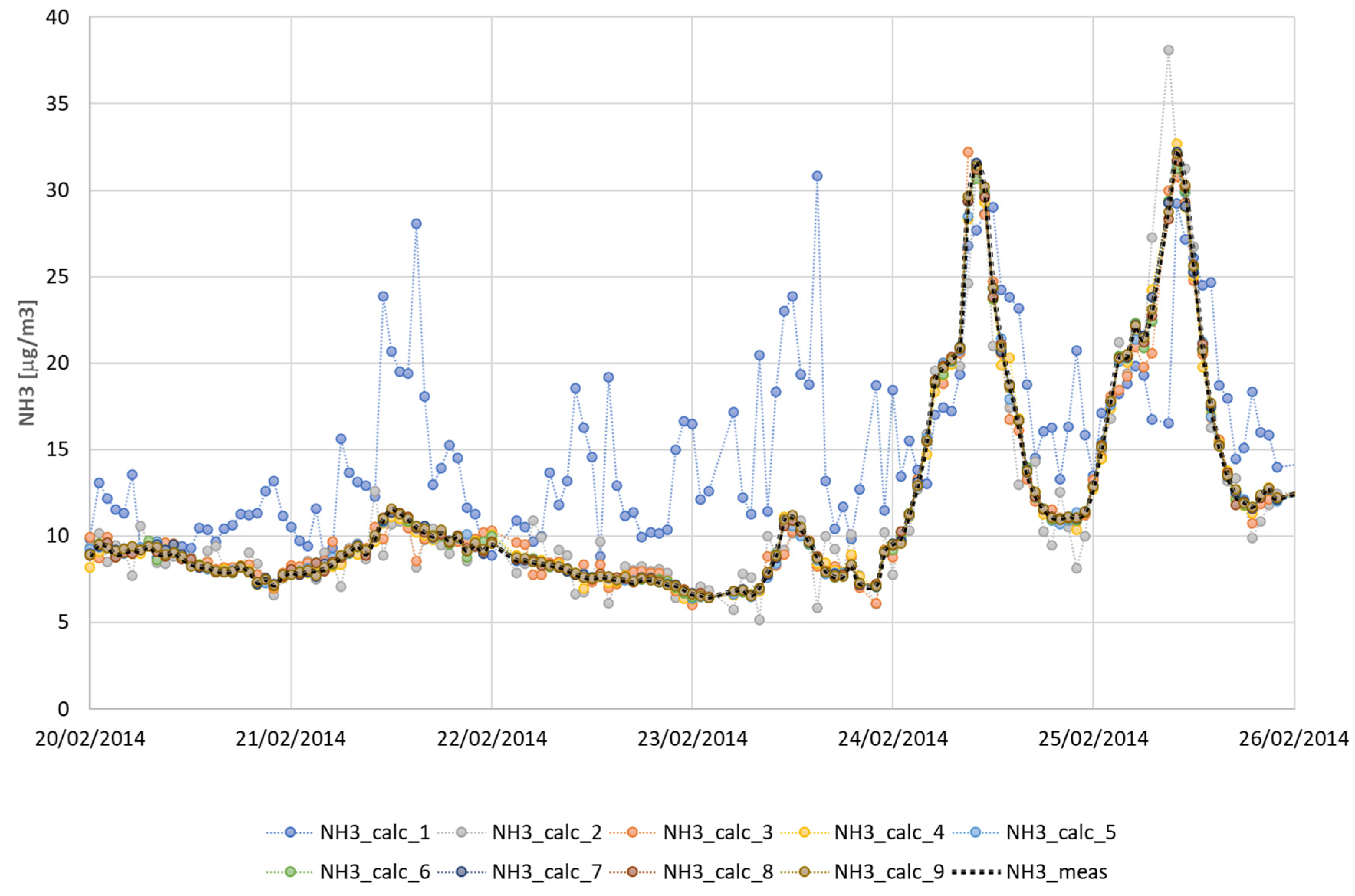
In the elaboration of training and test for each measurement site, the model performances for the predictions on the test subsets were quite similar to those obtained in the training phases. At the end of the first run the scatter plot between measured and calculated is “NH3_calc_1” and is reported in Figure 2.

The iteration proceeds with a second trial, where the first guess value for hourly emission flux of ammonia is multiplied by the ratio between measured and predicted concentrations. The procedures go as above described, with new random subsets, training and test. After each iteration the performances of the predictions progressively increase as shown in Figure 2, thanks to the refinements of the emissive input.

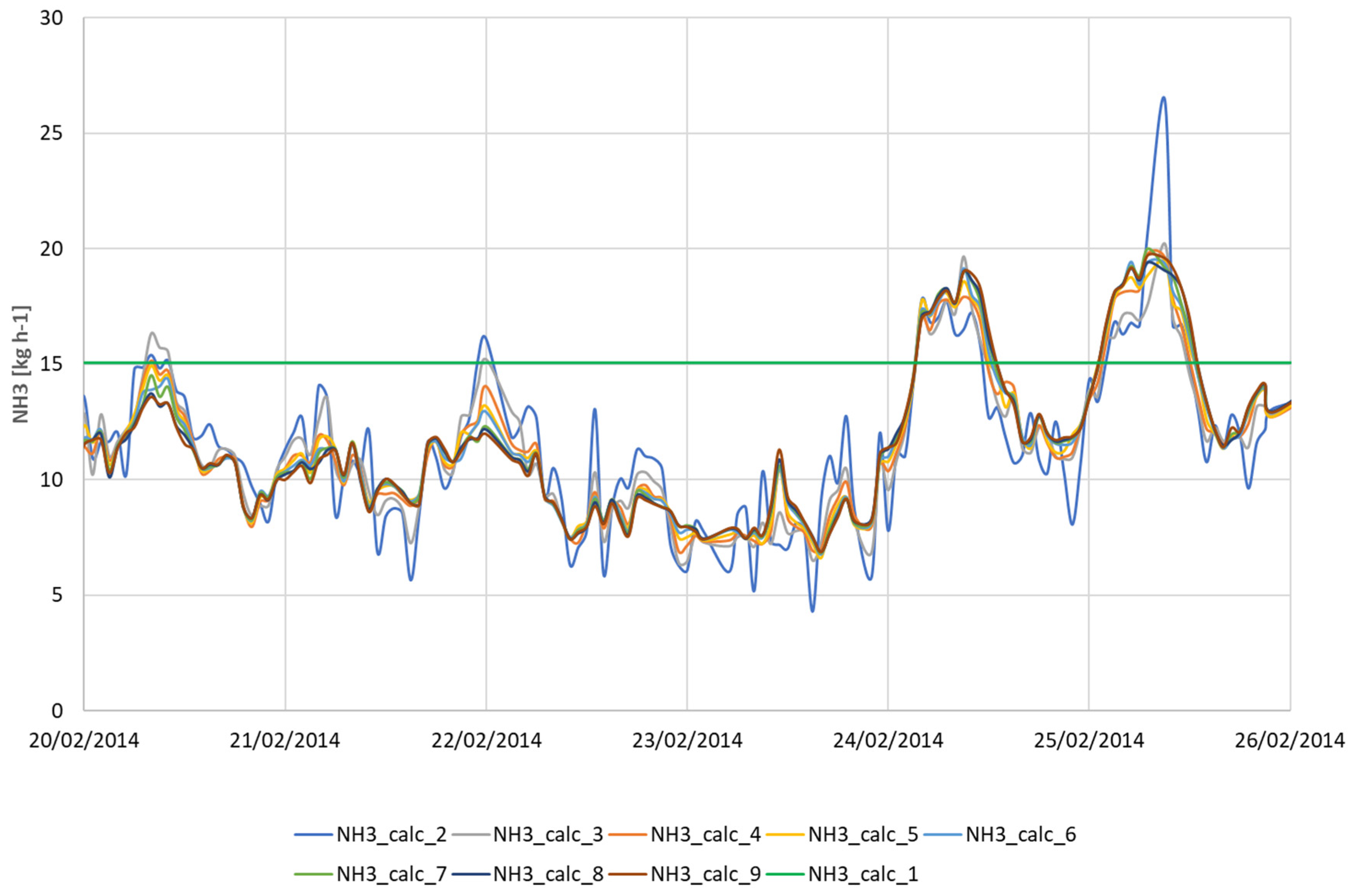
Figure 3 shows for the site of Schivenoglia (10_RB), focusing on a sample period, the estimated ammonia flux for each of the nine iterations.

Comparing the results of Figure 2 and Figure 3, the algorithm during the first training recognizes a group of atmospheric turbulence parameters favorable to the accumulation of ammonia in the atmosphere, for this reason the prediction obtained with constant emission in the first iteration of the methodology clearly overestimate the concentration compared with the measured ones.

During the day 21st, 22nd and 23rd February on the contrary the measured concentrations are very low compared with the predictions. In the second iteration and the subsequent ones the hourly emissions are then progressively corrected converging to a relative reduction from the starting value.

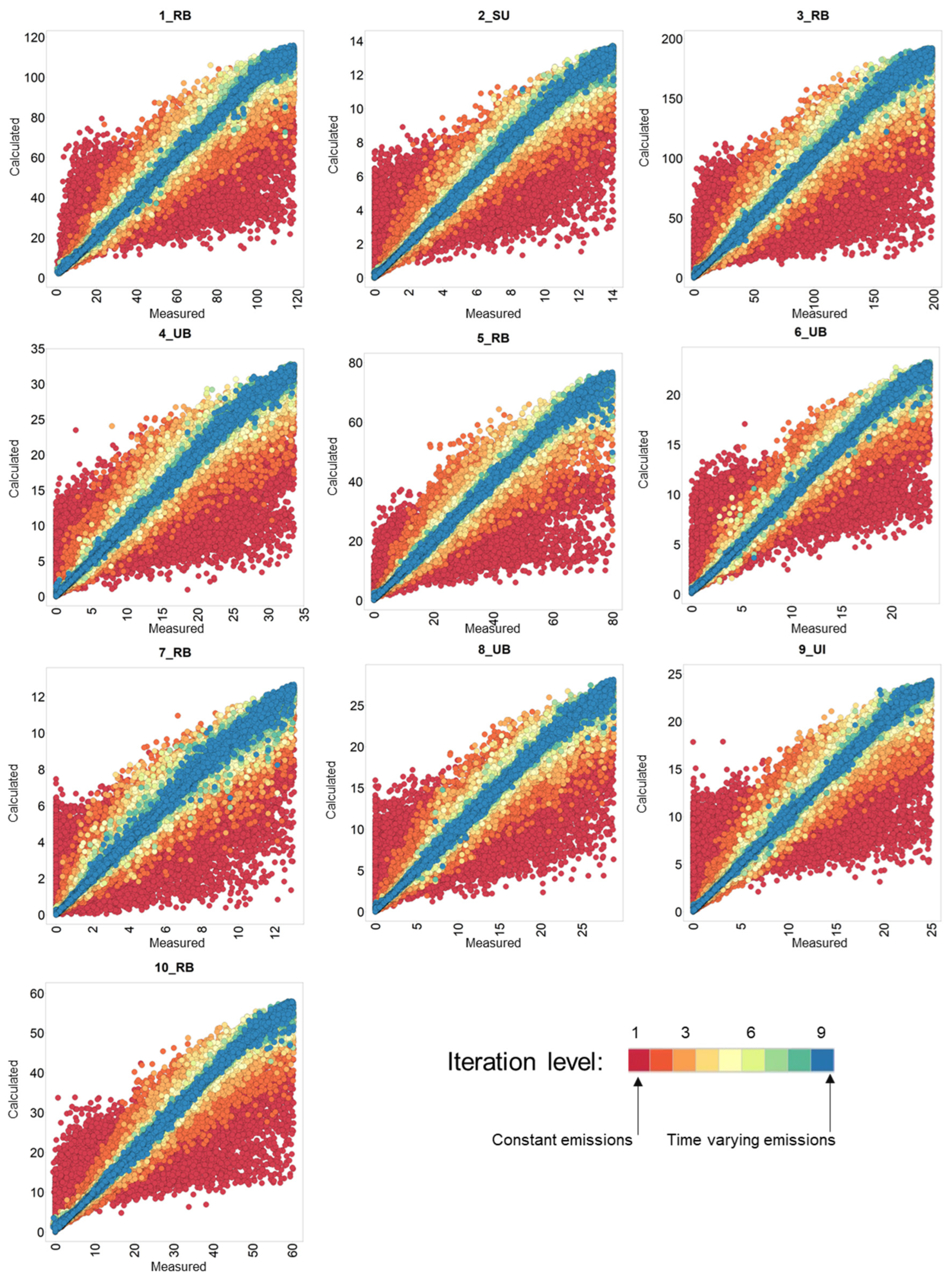
Figure 4 shows the progressive improvement of the comparison between predicted and measured concentrations by the iteration of the proposed methodology for each of the ten stations in northern Italy. The starting point is the constant emission scenario and it can be clearly seen how the iterations on the model show the same behavior for all the sites. Just moving to the second and third iteration the comparison between calculated and predicted will show a good correlation.

3. Results

The developed methodology consists in the solution of the inverse problem of estimating the ammonia emission rate in a restricted area nearby a monitoring station. The focused area can be restricted to few kilometers due to the physical and chemical properties of gaseous ammonia, lighter than air and reacting with water determining a fast decrease of concentration within the first 1-2 km from the sources [15].

The methodology calculates ammonia concentrations by similar atmospheric turbulence conditions and varying emission rate. In Figure 2, the first iteration NH₃_calc_1 predictions are only due to variability of the atmospheric conditions and do not consider real activity levels and other source specific variables, showing a sequence of different peaks of concentrations. From the second iteration, the hourly varying emissions are corrected and the predictions will vary smoothing some peaks.

The calculation of the emission rates joined to measured atmospheric concentrations is a common goal in solving inverse problem using Bayesian framework [45]. Also, in this case the authors restricted the domain to short-range transport using a Gaussian plume type solution as forward solver for transport of particles from fugitive sources. In the application of Bayesian framework, it was reported that authors would avoid the so called “inverse crime” [46]. The inverse crimes are when the numerical methods yield unrealistically optimistic results.

The link between emissions and concentrations has been examined to evaluate if the expected NH₃ concentrations and the calculated emissions are compatible with physical atmospheric turbulence parameters. The aforementioned methodology makes it possible to determine the site-specific NH₃ emissions for each hour of the dataset. On this dataset, a classification tree is used to take air turbulence parameters and time-varying observed concentrations into account. The applied methodology is available in the R package: “rpart” [47]. Using the decision tree, ammonia concentrations are classified as a function of atmospheric turbulence parameters. The classification thus obtained is then related to the estimated ammonia emission rates.

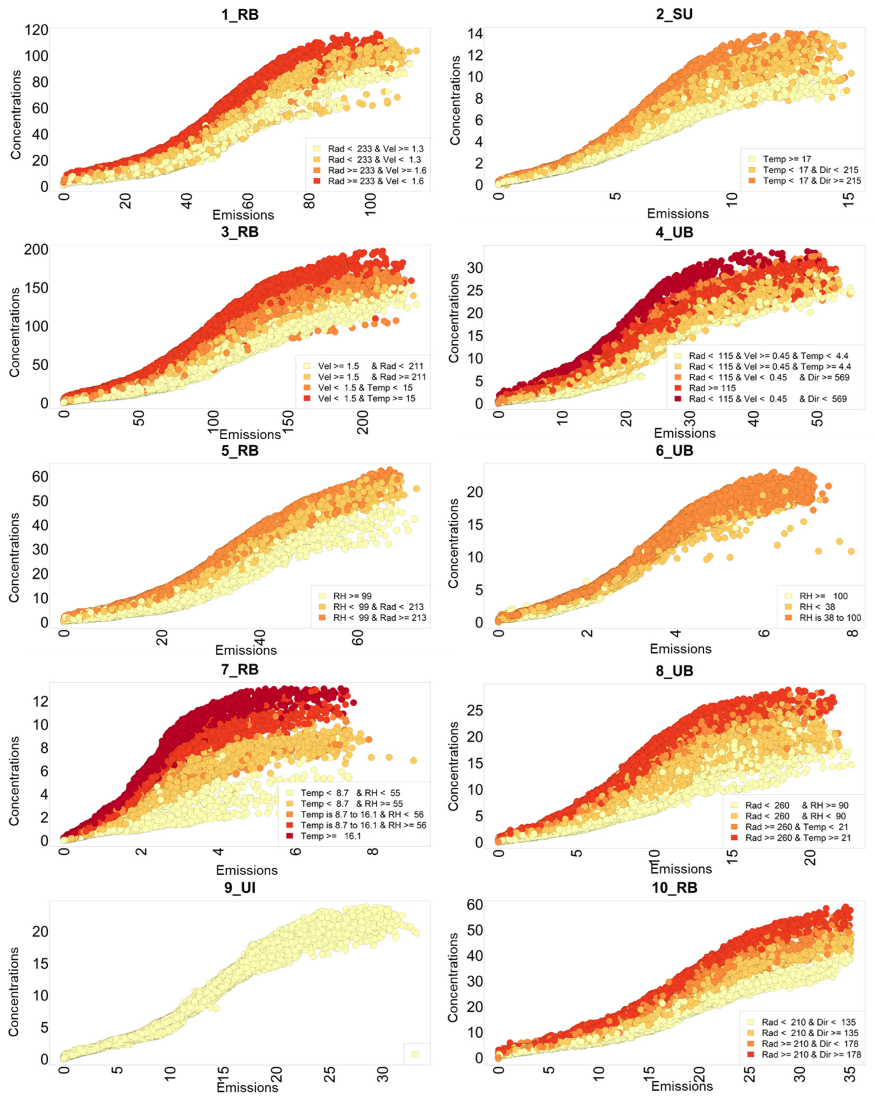
Figure 5 shows for each site, the variation of atmospheric concentrations of NH₃ with the increase of the calculated emission rates. The classification tree has identified different level of possible NH₃ atmospheric accumulation at a fixed emission level highlighting the possible role of meteorological conditions. The results seem to be reasonable from a physical point of view.

For station 1_RB in Figure 5, emission rate of 40 kg NH₃/h determines atmospheric concentrations in the range of 10-40 μg/m³. This variation can be explained considering the role of solar radiation and wind velocity. Higher values of solar radiation seem determining higher concentrations, at constant emissions. The role of wind velocity is identified, as a second actor, playing in a different way. At a fixed range of thermal radiation, higher wind strength will decrease the concentrations, allowing a better atmospheric dispersion.

By this analysis two sites, 2_SU and 10_RB, seem to be influenced also by wind direction, suggesting the presence of a specific source of ammonia emissions.

In the case of the industrial site 9_UI, the analysis was not able to identify specific turbulence pattern. For the remaining measuring stations higher temperatures, higher solar radiations and lower wind velocities seem favoring the accumulation of gaseous ammonia in the atmosphere.

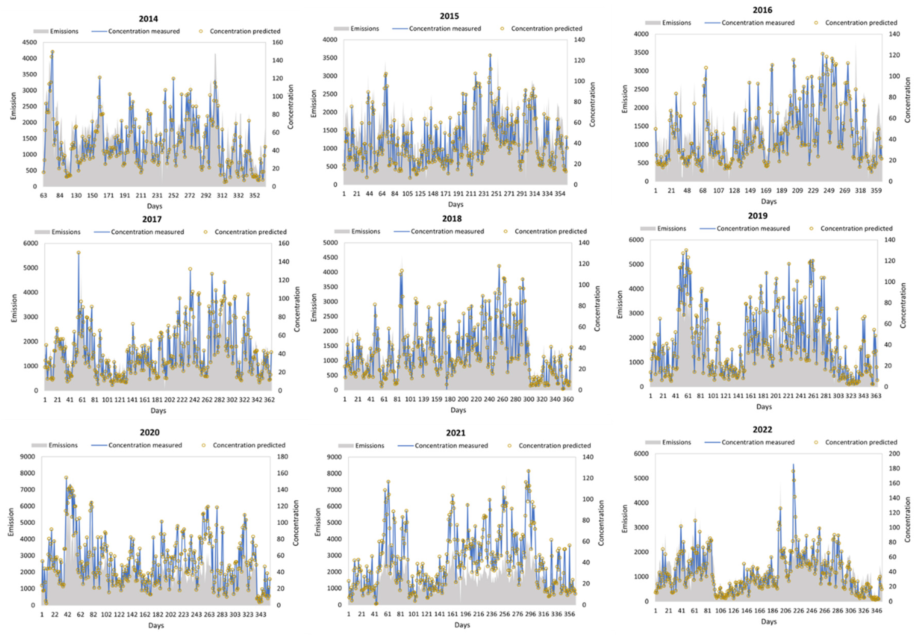
The proposed methodology allows the calculation of annual, monthly, and daily variation of the emission rate. As reported by Asman et al. [15] emission rate can show a peak in the afternoon related to warmer temperatures and higher turbulence. Farming operations can vary during the year reasonably showing peaks in Spring and Autumn. The ammonia daily concentrations during the years 2014-2022 in site 3_RB are shown in Figure 6. The comparison between the predictions and the data obtained by the measurements are in a very good agreement. The total emission rate is obtained summing the calculated ammonia emission for each day of the times series. The decoupling between emission rates and concentrations is more evident in some periods of the years 2020 and 2021, even the data from hourly base have been aggregated.

The comparison between emission rates and concentrations is based on real valid data, no data completion procedures are applied in Figure 6. The developed methodology is not affected by the absence of valid data which can be a more relevant issue in the calculation of annual and monthly total emission rate.

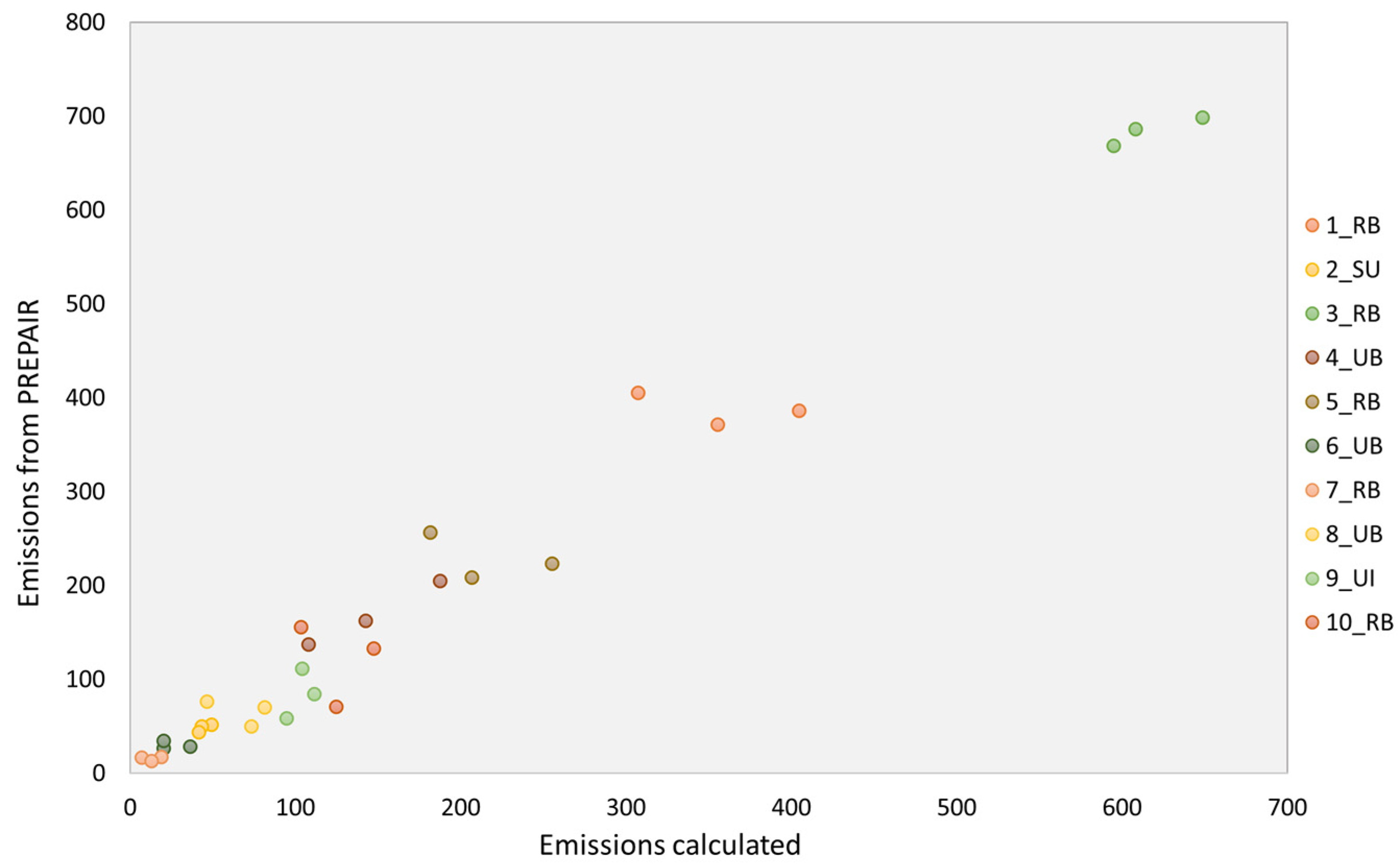
The data completion is considered in Figure 7. The total annual emission rate is calculated by applying a coefficient defined as the ratio between the total hours in the year and the number of valid data. Figure 7 clearly shows how the calculated emissions obtained by the methodology described in paragraph 2 are in very good agreement with the emission inventories of the PREPAIR Project. The spatial variation of emissions seems having a better agreement than time series for certain sites.

The motivation can be difficult to be defined, from one side the emission inventory is affected by different levels of uncertainties regarding emission factors and the annual and intra-annual fluctuation of the number of animals breaded. The field application of manure can be in different days of the year, even confined in the cultivation seasons, but also can occur not in the same municipality of the farm where the animals have produced the excreta nitrogen flow.

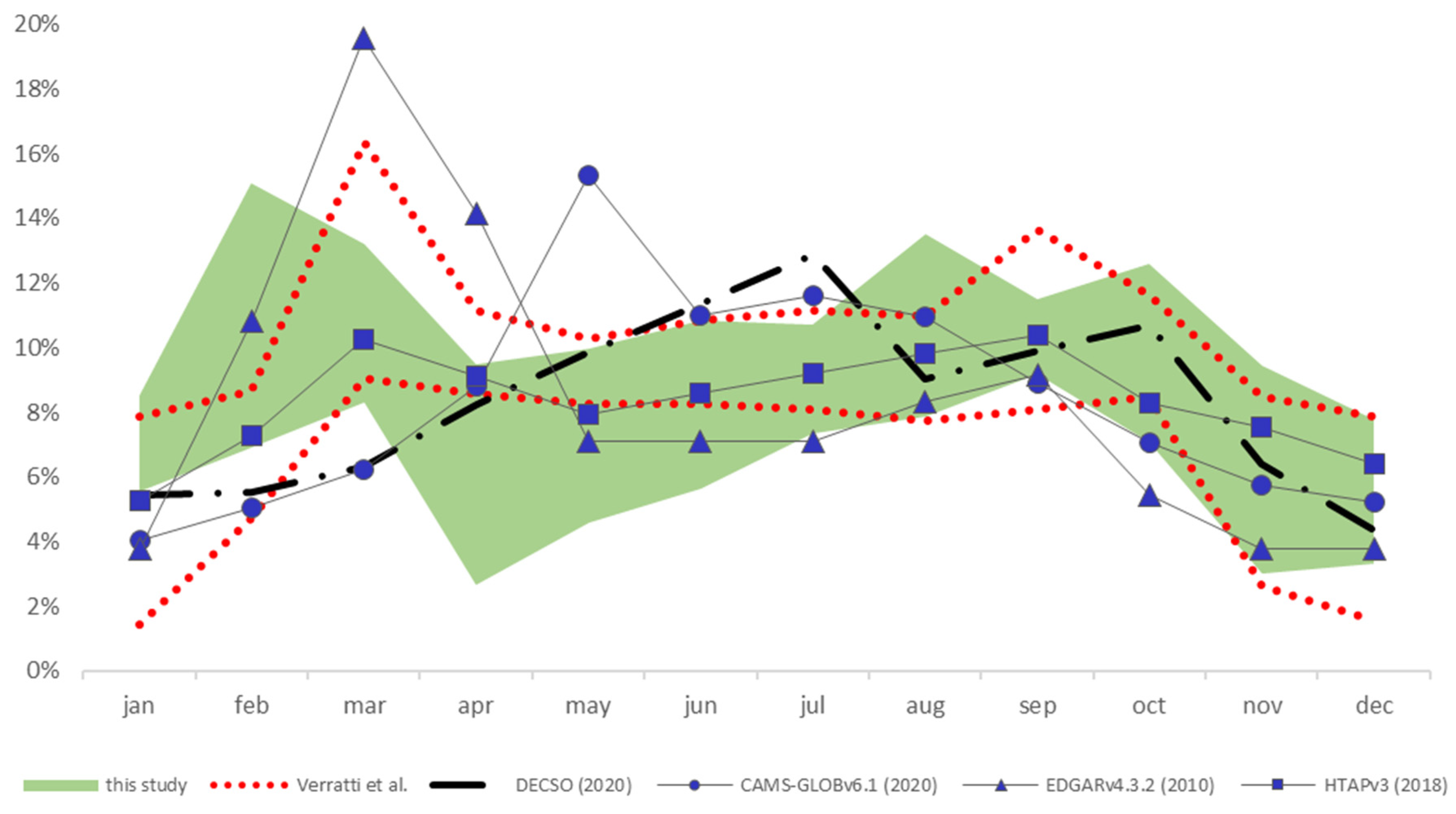
The air quality Chemical and Transport Models (CTMs) need the allocation of the annual emission inventory to hourly timesteps. The applied temporal patterns play an important role affecting the simulation results both in diagnostic and scenario elaborations. Veratti et al. [18] report an overview of the temporal distribution in Northern Italy of NH₃ emissions, applied by four different air quality modelling systems, based on three chemical transport models (CHIMERE, FARM and CAMx) [48,49,50,51,52,53,54]. The minimum and maximum monthly NH₃ emissions are reported in Figure 8 and compared to the calculation obtained by this study for the site 3_RB obtained considering the whole time series. These data are also compared with monthly emission profiles obtained from satellite observations and other global emission inventories.

The site 3_RB can be considered as representative of the area with higher emission density in the domain. The modelling emission profiles are quite in good agreement with the calculation obtained by this study. The main peaks are visible according to the period of field application of manure. The emissions calculated in this paper can show a wide variability in the years with the same order of magnitude of the range reported in the CTM modelling systems.

The method for estimating NH₃ emissions from satellite observations is an inversion technique that uses satellite observations and a chemical transport model: the DECSO v6.1 algorithm and CrIS observation. Free data are available on the SEEDS website, Sentinel EO-based Emission and Deposition Service [55], with a monthly temporal resolution for 2020 and a spatial resolution of 0.2 x 0.2 degrees (reported in Figure 8 as “DECSO”). The data are downloaded for the cell containing the site 3_RB. Data from CAMS Global anthropogenic emissions (reported as “CAMS-GLOB v6.1”), Hemispheric Transport of Air Pollution emission inventory (reported as “HTAP v3”), and EDGAR global monthly gridded anthropogenic emissions (reported as “EDGAR v4.3.2”) are all obtained from the Emissions of Atmospheric Compounds and Compilation of Ancillary Data website [56] and extrapolated by selecting the cell containing the site 3_RB.

The spatial resolution of the CAMS-GLOB inventory [57] is 0.1 × 0.1 degrees and is based on EDGAR v4.3.2 annual emissions for the years 2000-2012, where monthly temporal profiles from CAMS-GLOB-TEMPO were applied. After 2012, monthly emissions are extrapolated to the current year using linear trends fit to the years 2011-2014 from the CEDS global inventory. HTAP v3 [58] is an ad hoc global mosaic of anthropogenic inventories that combines official inventories for specific areas such as North America, Europe, Asia including Japan and Korea with the independent Emissions Database for Global Atmospheric Research (EDGAR) inventory for the remaining regions of the world. The results are spatially and temporally distributed emissions with a spatial resolution of 0.1 × 0.1 degrees and time intervals of months and years covering the period 2000–2018. For Europe, emission grid maps have been collected from officially reported data, specifically from EMEP for Europe (CAMS-REG-v5.1). The scientific global emission inventory EDGAR v4.3.2[59] provides a dataset of anthropogenic emissions of gaseous and particulate air pollutants with annual and monthly resolution in 1970–2012 and spatially disaggregated grid maps with a resolution of 0.1 × 0.1 degrees.

4. Discussion

The phenomenology of NH₃ release and its accumulation in the atmosphere can be affected by several variables. Some of these are measured or calculated by modelling systems for describing the turbulence of the atmosphere. In this study, a machine learning methodology for estimating emission rates based on these variables has been implemented. The proposed iterative process for the determination of the emission rate of NH₃ tries to separate the effects of meteorology from the variation in space and time of the overall effects of the emission sources.

Each subsequent iteration improves the ability to predict ammonia concentrations, that is, gradually as the self-learning process, inherent in the methodology itself and is strengthened from time to time by analyzing new data.

The proposed methodology provides a very good description of the ammonia concentrations measured by stations and their variability over time linked to the estimated emission rates.

The emission rates calculated in this study are compared with the main results of the emission inventories estimated on the investigated area both considering their spatial and temporal variation. This comparison, with very encouraging results, is very important to ensure consistency between the estimated data, on hourly base, with the available and estimated independently data, extracted in the same site, but on an annual scale.

Further analysis involved the monthly emission profiles estimated by the study, which agree with the main assumptions documented in air quality modeling or in inverse calculations from satellite observations and modeling simulations.

The same profiles are also reasonable considering seasonal variation of temperature and solar rations and the possible program in agriculture activities. Different behavior and comparison can be obtained considering high time and spatial resolution of the calculated emission rates. Moving to very detailed scale and to the hourly time resolution the emission profile can show very high variability. Only a minor part of this variability can be explained by atmospheric turbulence parameters, and it can be reasonably linked to changes in the emission sources. At a very local scale, the field application of manure can occur in different period of the year even on the same season and can be affected also by different parameters. The local presence of a certain number of livestock units cannot be always linked to the emissions of ammonia in all the manure management phases, being the possible treatment and field application not always located in proximity of the housing structure.

As a matter of facts, the analysis of measured ammonia concentrations does not show a recursive pattern, suggesting that at a very local scale the ammonia emission rate and its time series can be very variable. This aspect must be considered in the development of bottom-up emission inventories and in their use and application in air quality simulations.

The proposed approach is suitable for being extended to further applications, considering the possible interactions of gaseous ammonia with other ammonia like components and with reacting atmospheric acid gases in the possible formation of ultrafine particulate matter. A further possible extension of this paper is the analysis with this methodology on the determination of time series for specific atmospheric tracers or contaminants like levoglucosan, for biomass burning sources and heavy metals, for specific emission sources.

Supplementary Materials

The following supporting information can be downloaded at the website of this paper posted on Preprints.org, Table S1: for each reference site, the correlation matrix in percentage between meteorological turbulence variables and ammonia concentration divided into quartiles.

Author Contributions

Conceptualization, A.M. and E.A.; methodology, A.M.; software, A.M. and G.G.D.; validation, A.M., A.G.C. and G.G.D; formal analysis, A.M.; investigation, A.M., G.G.D and A.G.C.; resources, A.M.; data curation, A.M., G.G.D and A.G.C.; writing—original draft preparation, A.M., G.G.D and A.G.C.; writing—review and editing, E.A. and A.M.; visualization, , A.M., G.G.D and A.G.C.; supervision, A.M.; project administration, E.A.; funding acquisition, E.A. All authors have read and agreed to the published version of the manuscript.

Funding

This research was funded by LIFE-IP PREPAIR (Po Regions Engaged to Policies of AIR) project, Grant Number LIFE15 IPE/IT/000013 and by REGIONE LOMBARDIA with “Progetto di monitoraggio ammoniaca dal comparto agricolo 2022/2023” identification code n. 2022.0043891 - 18/03/2022.

Informed Consent Statement

Not applicable.

Data Availability Statement

The dataset with updated emission estimates on Lombardy is available to the public: https://www.inemar.eu/xwiki/bin/view/Inemar/HomeLombardia. Details on methodologies and emission factors are available to the public: http://www.inemar.eu/xwiki/bin/view/FontiEmissioni/.

Acknowledgments

Acknowledgments are given to all the Beneficiaries of the LIFE-IP PREPAIR: Emilia-Romagna Region (Project Coordinator) Veneto Region, Lombardy Region, Piedmont Region, Friuli Venezia Giulia Region, Autonomous Province of Trento, Regional Agency for Environment of Emilia-Romagna (ARPAE), Regional Agency for Environment of Veneto, Regional Agency for Environment of Piedmont, Regional Agency for Environmental Protection of Lombardy, Environmental Protection Agency of Valle d’Aosta, Environmental Protection Agency of Friuli Venezia Giulia, Slovenian Environment Agency, Municipality of Bologna, Municipality of Milan, City of Turin, ART-ER, Lombardy Foundation for Environment.

Conflicts of Interest

The authors declare no conflict of interest.

References

Backes, A.; Aulinger, A.; Bieser, J.; Matthias, V.; Quante, M. Ammonia emissions in Europe, part I: Development of a dynamical ammonia emission inventory. Atmospheric Environment 2016, 131, 55–66. [Google Scholar] [CrossRef]
Hempel, S.; Adolphs, J.; Landwehr, N.; Janke, D.; Amon, T. How the Selection of Training Data and Modeling Approach Affects the Estimation of Ammonia Emissions from a Naturally Ventilated Dairy Barn—Classical Statistics versus Machine Learning. Sustainability 2020, 12. [Google Scholar] [CrossRef]
Amon, B.; Kryvoruchko, V.; Amon, T.; Zechmeister-Boltenstern, S. Methane, nitrous oxide and ammonia emissions during storage and after application of dairy cattle slurry and influence of slurry treatment. Agriculture, Ecosystems & Environment 2006, 112, 153–162. [Google Scholar] [CrossRef]
Monteny, G. J.; Groenestein, C. M.; Hilhorst, M. A. Interactions and coupling between emissions of methane and nitrous oxide from animal husbandry. Nutrient Cycling in Agroecosystems 2001, 60, 123–132. [Google Scholar] [CrossRef]
Hristov, A. N. Technical note: Contribution of ammonia emitted from livestock to atmospheric fine particulate matter (PM2.5) in the United States. Journal of Dairy Science 2011, 94, 3130–3136. [Google Scholar] [CrossRef]
Vries, de W.; Grinsven HJM, van; contributions from Ayyappan, with S.; Fichelet, P. V. Published by the Centre for Ecology and Hydrology (CEH), Edinburgh UK, on behalf of the Global Partnership on Nutrient Management (GPNM) and the International Nitrogen Initiative (INI).) Our Nutrient World: The challenge to produce more food and energy with less pollution. Global Overview of Nutrient Management. Centre for Ecology and Hydrology, Edinburgh on behalf of the Global Partnership on Nutrient Management and the International Nitrogen Initiative. 2013.
Hempel, S.; Menz, C.; Pinto, S.; Galán, E.; Janke, D.; Estellés, F.; et al. Heat stress risk in European dairy cattle husbandry under different climate change scenarios-uncertainties and potential impacts. Earth System Dynamics 2019, 10, 859–884. [Google Scholar] [CrossRef]
DIRECTIVE (EU) 2016/ 2284 - on the Reduction of National Emissions of Certain Atmospheric Pollutants, Amending Directive 2003/ 35/ EC and Repealing Directive 2001/ 81/ EC; European Parliament: EU, 2016.
EMEP/EEA Air Pollutant Emission Inventory Guidebook 2016: Technical Guidance to Prepare National Emission Inventories; Office of the European Union: Luxembourg, 2016.
EMEP/EEA Air Pollutant Emission Inventory Guidebook 2019: Technical Guidance to Prepare National Emission Inventories; Publications Office of the European Union: Luxembourg, 2019.
11. European Union Emission Inventory Report 1990/2019. Office of the European Union: Luxembourg, 2021.
Italian Emission Inventory 1990 – 2019. Informative Inventory Report 2021.; ISPRA IIR: Roma, 2021; Available online: www.isprambiente.gov.it.
Marongiu, A.; Angelino, E.; Moretti, M.; Malvestiti, G.; Fossati, G. Atmospheric Emission Sources in the Po-Basin from the LIFE-IP PREPAIR Project. Open Journal of Air Pollution 2013, 11, 70–83. [Google Scholar] [CrossRef]
BDN – Anagrafe Nazionale Zootecnica. https://www.vetinfo.it/j6_statistiche/#/.
Asman, W. A. H.; Sutton, M. A.; Schjørring, J. K. Ammonia: emission, atmospheric transport and deposition. New Phytologist 1998, 139, 27–48. [Google Scholar] [CrossRef]
Asman, W. A. H. Ammonia emission in Europa: Updated emission and emission variations. 1992.
Thunis, P.; Clappier, A.; Beekmann, M.; Putaud, J. P.; Cuvelier, C.; Madrazo, J.; et al. Non-linear response of PM2.5 to changes in NOx and NH3 emissions in the Po basin (Italy): Consequences for air quality plans. Atmospheric Chemistry and Physics 2021, 21, 9309–9327. [Google Scholar] [CrossRef]
Veratti, G.; Stortini, M.; Amorati, R.; Bressan, L.; Giovannini, G.; Bande, S.; et al. Impact of NOx and NH3 Emission Reduction on Particulate Matter across Po Valley: A LIFE-IP-PREPAIR Study. Atmosphere 2023, 14, 762. [Google Scholar] [CrossRef]
Hutchings, N. J.; Sommer, S. G.; Andersen, J. M.; Asman, W. A. H. A detailed ammonia emission inventory for Denmark. Atmospheric Environment 2001, 35, 1959–1968. [Google Scholar] [CrossRef]
Ambelas SkjøTh, C.; Hertel, O.; GyldenkæRne, S.; Ellermann, T.; Ambelas SkjøTh, C.; Hertel, O.; et al. Implementing a dynamical ammonia emission parameterization in the large-scale air pollution model ACDEP. JGRD 2004, 109, D06306. [Google Scholar] [CrossRef]
Gyldenkærne, S.; Skjøth, C. A.; Hertel, O.; Ellermann, T. A dynamical ammonia emission parameterization for use in air pollution models. Journal of Geophysical Research Atmospheres 2005, 110, 1–14. [Google Scholar] [CrossRef]
Huang, X.; Song, Y.; Li, M.; Li, J.; Huo, Q.; Cai, X.; et al. A high-resolution ammonia emission inventory in China. Global Biogeochemical Cycles 2012, 26. [Google Scholar] [CrossRef]
Sutton, P.; Chemel, C.; Griffiths, S.; Sokhi, R. S. Investigation, using CMAQ, of sensitivity of air quality modelling to input ammonia emissions. In Air Pollution Modeling and its Application XXII; 2012; Vol. 96.
Reis, S.; Ambelas-Skjoth, C.; Vieno, M.; Geels, C.; Steinle, S.; Lang, M.; et al. Why time and space matters-arguments for the improvement of temporal emission profiles for atmospheric dispersion modeling of air pollutant emissions. In 19th International Congress on Modelling and Simulation; Perth, Australia, 2011.
Van Der Gon, H. D.; Hendriks, C.; Kuenen, J.; Segers, A.; Visschedijk, A. Description of Current Temporal Emission Patterns and Sensitivity of Predicted AQ for Temporal Emission Patterns EU FP7 MACC Deliverable Report D_D-EMIS_1.3; 2011.
Arogo, J.; Zhang, R. H.; Riskowski, G. L.; Christianson, L. L.; Day, D. L. Mass Transfer Coefficient of Ammonia in Liquid Swine Manure and Aqueous Solutions. Journal of Agricultural Engineering Research 1999, 73, 77–86. [Google Scholar] [CrossRef]
Cortus, E. L.; Lemay, S. P.; Barber, E. M.; Hill, G. A. Modelling ammonia emission from swine slurry based on chemical and physical properties of the slurry. Can Biosyst Eng, 2009, 51, 6–9. [Google Scholar]
de Visscher, A.; Harper, L. A.; Westerman, P. W.; Liang, Z.; Arogo, J.; Sharpe, R. R.; et al. Ammonia Emissions from Anaerobic Swine Lagoons: Model Development. JApMe 2002, 41, 426–433. [Google Scholar] [CrossRef]
Sommer, S. G.; Christensen, M. L.; Schmidt, T.; Jensen, L. S. Animal Manure Recycling - Treatment and Management; Sommer, S. G., Christensen, M. L., Schmidt, T., Jensen, L. S., Eds.; John Wiley & Sons Ltd: West Sussex, United Kingdom, 2013. [Google Scholar]
Sommer, S. G.; Zhang, G. Q.; Bannink, A.; Chadwick, D.; Misselbrook, T.; Harrison, R.; et al. Algorithms determining ammonia emission from buildings housing cattle and pigs and from manure stores. Advances in Agronomy 2006, 89, 261–335. [Google Scholar] [CrossRef]
Teye, F. K.; Hautala, M. Adaptation of an ammonia volatilization model for a naturally ventilated dairy building. Atmospheric Environment 2008, 42, 4345–4354. [Google Scholar] [CrossRef]
Wang, Z.; Zhang, R.; Mansell, G.; Fadel, J.; Rumsey, T.; Xin, H.; et al. Development of an Improved Process-Based Ammonia Model for Agricultural Sources; 2005. Available online: https://www.researchgate.net/publication/265880715.
Wang, C. Y.; Li, B. M.; Zhang, G. Q.; Rom, H. B.; Shi, Z. X. Comparison between the Statistical Method and Artificial Neural Networks in Estimating Ammonia Emissions from Naturally Ventilated Dairy Cattle Buildings. In Livestock Environment VIII - Proceedings of the 8th International Symposium; American Society of Agricultural and Biological Engineers, 2009; pp 7-. [CrossRef]
Boniecki, P.; Dach, J.; Pilarski, K.; Piekarska-Boniecka, H. Artificial neural networks for modeling ammonia emissions released from sewage sludge composting. Atmospheric Environment 2012, 57, 49–54. [Google Scholar] [CrossRef]
Stamenković, L. J.; Antanasijević, D. Z.; Ristić, M.; Perić-Grujić, A. A.; Pocajt, V. V. Modeling of ammonia emission in the USA and EU countries using an artificial neural network approach. Environmental science and pollution research international 2015, 22, 18849–18858. [Google Scholar] [CrossRef]
Liakos, K. G.; Busato, P.; Moshou, D.; Pearson, S.; Bochtis, D. Machine Learning in Agriculture: A Review. Sensors 2018, 18, 2674. [Google Scholar] [CrossRef]
Fassò, A.; Rodeschini, J.; Moro, A. F.; Shaboviq, Q.; Maranzano, P.; Cameletti, M.; et al. Agrimonia: a dataset on livestock, meteorology and air quality in the Lombardy region, Italy. Scientific Data 2023, 10. [Google Scholar] [CrossRef]
Hemant Ishwaran; Udaya B. Kogalur. Fast Unified Random Forests for Survival, Regression, andClassification (RF-SRC). 2023. Accessed 23.04.01. Available online: https://www.randomforestsrc.org/; https://ishwaran.org/.
Ishwaran, H.; Kogalur, U. B. Random Survival Forests for R. 2007, 7.
Ishwaran, H.; Kogalur, U. B.; Blackstone, E. H.; Lauer, M. S. RANDOM SURVIVAL FORESTS 1. The Annals of Applied Statistics 2008, 2, 841–860. [Google Scholar] [CrossRef]
Ishwaran, H.; Lu, M.; Lauer, M. S.; Blackstone, E. H.; Kogalur, U. B. randomForestSRC: Getting Started with randomForestSRC Vignette. 2021. Accessed 23.06.22. Available online: http://randomforestsrc.org/articles/survival.html.
Breiman, L. Random Forests; 2001; Vol. 45.
Ho, T. K. Random decision forests. Proceedings of the International Conference on Document Analysis and Recognition, ICDAR 1995, 1, 278–282. [Google Scholar] [CrossRef]
Breiman, L. Using_random_forests_v4.0.
Hosseini, B.; Stockie, J. M. Bayesian estimation of airborne fugitive emissions using a Gaussian plume model. Atmospheric Environment 2016, 141, 122–138. [Google Scholar] [CrossRef]
Kaipio, J.; Somersalo, E. Statistical and Computational Inverse Problems; Applied Mathematical Sciences; Springer New York, 2006.
Therneau, T.; Atkinson, B.; Ripley, B. Recursive Partitioning and Regression Trees. 2022. Available online: https://cran.r-project.org/package=rpart.
Mailler, S.; Menut, L.; Khvorostyanov, D.; Valari, M.; Couvidat, F.; Siour, G.; et al. CHIMERE-2017: from urban to hemispheric chemistry-transport modeling. Geosci. Model Dev. 2017, 10, 2397–2423. [Google Scholar] [CrossRef]
Menut, L.; Bessagnet, B.; Briant, R.; Cholakian, A.; Couvidat, F.; Mailler, S.; et al. The CHIMERE v2020r1 online chemistry-transport model. Geosci. Model Dev. 2021, 14, 6781–6811. [Google Scholar] [CrossRef]
Gariazzo, C.; Silibello, C.; Finardi, S.; Radice, P.; Piersanti, A.; Calori, G.; et al. A gas/aerosol air pollutants study over the urban area of Rome using a comprehensive chemical transport model. Atmospheric Environment 2007, 41, 7286–7303. [Google Scholar] [CrossRef]
Silibello, C.; Calori, G.; Brusasca, G.; Giudici, A.; Angelino, E.; Fossati, G.; et al. Modelling of PM10 concentrations over Milano urban area using two aerosol modules. Environ. Model. Softw. 2008, 23, 333–343. [Google Scholar] [CrossRef]
Dalla-Fontana, A.; Pillon, S.; Patti, S. A performance evaluation of the CAMx air quality model to forecast ozone and PM10 over the Italian region of Veneto. Tethys 2021, 18, 1–13. [Google Scholar] [CrossRef]
Ciarelli, G.; Aksoyoglu, S.; Crippa, M.; Jimenez, J.-L.; Nemitz, E.; Sellegri, K.; et al. Evaluation of European air quality modelled by CAMx including the volatility basis set scheme. Atmospheric Chemistry and Physics 2016, 16, 10313–10332. [Google Scholar] [CrossRef]
Nopmongcol, U.; Koo, B.; Tai, E.; Jung, J.; Piyachaturawat, P.; Emery, C.; et al. Modeling Europe with CAMx for the Air Quality Model Evaluation International Initiative (AQMEII). Atmospheric Environment 2012, 53, 177–185. [Google Scholar] [CrossRef]
Sentinel EO-based Emission and Deposition Service - SEEDS. Accessed 23.05.05. Available online: https://www.seedsproject.eu/data/monthly-nh3-emissions.
Emissions of atmospheric Compounds and Compilation of Ancillary Data - ECCAD. Accessed 23.05.08. Available online: https://eccad.sedoo.fr/#/catalogue.
Granier, C.; Darras, S.; Denier Van Der Gon, H.; Jana, D.; Elguindi, N.; Bo, G.; et al. The Copernicus Atmosphere Monitoring Service Global and Regional Emissions (April 2019 Version); 2019. Available online: https://hal.science/hal-02322431v2.
Crippa, M.; Guizzardi, D.; Butler, T.; Keating, T.; Wu, R.; Kaminski, J.; et al. HTAP_v3 emission mosaic: a global effort to tackle air quality issues by quantifying global anthropogenic air pollutant sources. Earth System Science Data Discussions 2023, 1–34. [Google Scholar] [CrossRef]
Crippa, M.; Guizzardi, D.; Muntean, M.; Schaaf, E.; Dentener, F.; van Aardenne, J. A.; et al. Gridded emissions of air pollutants for the period 1970–2012 within EDGAR v4.3.2. Earth System Science Data 2018, 10, 1987–2013. [Google Scholar] [CrossRef]

Figure 1. Emission density map in northern Italy and ammonia concentrations measurement sites considered in this study.

Figure 2. Focus on a short period for station 10_RB, comparison between predicted and measured concentrations of NH3 for each model iteration.

Figure 3. Focus on a short period for station 10_RB, variation of estimated emission flux for each model iteration.

Figure 4. Comparison between the measured NH₃ atmospheric concentrations and the predicted ones [μg/m³] at each step of the iteration for the different sites in Northern Italy. Each color corresponds to an iteration.

Figure 5. Relation between ammonia estimated emissions expressed in kg NH₃/h and predicted ammonia concentrations [μg/m³] as function of turbulence atmospheric parameters.

Figure 6. Time series of daily average concentrations of measured and predicted ammonia [μg/m³] and total daily emissions for 3_RB [kg NH₃/day].

Figure 7. Total annual emission of ammonia [t/year] in different sites for three years: 2013-2017-2019, comparison between calculated data by this study and emission inventories in the PREPAIR Project.

Figure 8. NH₃ monthly emissions variability between calculated in this study and different available sources expressed as ratio between monthly and annual emissions for a fixed year.

Table 1. Ammonia measurements sites, average measured ammonia and wind velocity, annual surrounding emissions estimates and main emissions macrosectors.

Id-Station	Measurement Site	NH₃ (µg/m³)	Wind velocity (m/s)	NH₃ t/year 2014	NH₃ t/year 2017	Agriculture (%) 2017	Road transport (%) 2017	Other sources (%) 2017	NH₃ t/year 2019
1_RB	Bertonico	33.65	1.46	404.9	385.9	99.2	0.2	0.6	371.4
2_SU	Colico	4.36	1.26	51.6	50.0	94.1	1.8	4.1	43.8
3_RB	Corte de Cortesi	44.5	1.9	698.4	685.9	99.7	0.1	0.2	668.4
4_UB	Cremona – Via Fatebenefratelli	8.78	1.12	205.0	162.1	95.9	2.6	1.5	137.2
5_RB	Cremona – Via Gerre Borghi	15.41	1.16	256.3	222.9	98.0	1.2	0.8	208.6
6_UB	Milano – Pascal Città Studi	9.08	1.82	26.5	28.2	47.6	41.3	11.1	34.2
7_RB	Moggio	2.77	1.21	16.9	17.4	86.5	4.7	8.9	13.2
8_UB	Pavia – Via Folperti	7.7	1.11	49.7	70.2	87.6	4.5	7.9	76.3
9_UI	Sannazzaro de’ Burgondi	8.38	2.23	58.5	111.4	57.8	0.8	41.4	84.0
10_RB	Schivenoglia	16.27	1.68	155.7	132.9	98.3	0.4	1.3	70.9

Disclaimer/Publisher’s Note: The statements, opinions and data contained in all publications are solely those of the individual author(s) and contributor(s) and not of MDPI and/or the editor(s). MDPI and/or the editor(s) disclaim responsibility for any injury to people or property resulting from any ideas, methods, instructions or products referred to in the content.

© 2023 by the authors. Licensee MDPI, Basel, Switzerland. This article is an open access article distributed under the terms and conditions of the Creative Commons Attribution (CC BY) license (http://creativecommons.org/licenses/by/4.0/).

Copyright: This open access article is published under a Creative Commons CC BY 4.0 license, which permit the free download, distribution, and reuse, provided that the author and preprint are cited in any reuse.

MDPI Initiatives

Important Links

Choose an area of interest and we will send you notifications of new preprints at your preferred frequency.

Disclaimer