1. Introduction
The last two decades have witnessed the rapid growth of wearable devices, increasingly being used for ubiquitous health monitoring. Human activity recognition (HAR) aims at detecting simple behaviours such as walking or gestures and more complex behaviours like cooking or opening a door with various use-cases that continue to grow as the field expands; assistive technology, such as identifying odd behaviours in the elderly, including falls [
1], skill assessment [
2], helping with rehabilitation [
3], sports injury detection, and ambient assisted living [
4,
5,
6]. Accurately predicting human activities from sensor data is difficult due to the complexity of human behaviour and the noise in the sensor data [
7].
With larger datasets and more computational power, deep learning has evolved, removing the need for manually created features and inductive biases from models and increasing the reliance on automatically learning features from raw labelled data [
8]. Complex deep learning techniques, such as convolutions and attention-based mechanisms, are used increasingly with growing computational capacity. These techniques perform well with larger models resulting in processes that are generally more expensive computationally and memory-wise than previous techniques. Although wearable devices and smartphones have rapidly increased in computation efficiency over the past two decades, they are still limited in power and storage; this prevents them from using state-of-the-art deep learning techniques in HAR.
MLP-Mixers, recently created by Google Brain [
8], are simplistic and less computationally expensive models, yet they produce near state-of-the-art results in computer vision tasks. Wearable devices could produce competitive results in HAR without the significant computational demands that current state-of-the-art models impose if MLP-Mixers performed similarly in HAR which would help advance HAR toward low-powered devices.
The main contributions of this paper are as follows:
We investigate the performance of the MLP-Mixer in multi-sensor HAR achieving competitive, and in some cases, state-of-the-art performance in HAR without convolution, recurrent or attention-based mechanisms in the model.
We analyse the impact of each layer in the Mixer for HAR.
We analyse the effect of the sliding windows on the Mixer’s performance in HAR.
We perform a visual analysis of the Mixer’s weights to validate that the Mixer is successfully recognising different human activities.
2. Related Work
Four main categories of deep-learning architecutres have been used in HAR, convolution-based architectures, recurrent networks, hybrid models, and attention-based models [
9]. Evaluation is performed on benchmark HAR datasets including Opportunity [
10], Daphnet Gait [
11], PAMAP2 [
12], Skoda Checkpoint [
13], WISDM [
14], MHEALTH [
15,
16] and UCI-HAR [
17].
With the recent success of CNNs in feature detection, Zeng et al. [
18] first proposed using CNNs in HAR, but they only used a basic CNN on a single accelerometer. Next, Hammerla et al. [
19] thoroughly investigated CNN use in HAR and established its viability. However, good performance requires large CNN models or residual CNNs [
20]; this increases the computational cost, constraining their use on low-power devices. To solve this, Tang et al. [
21] looked into the performance and viability of an efficient CNN that uses a tiny Lego filter inspired by Yang et al. [
22]. The paper investigated a resource-constrained CNN model for HAR on mobile and wearable devices achieving an
score of 91.40% and 86.10% in the PAMAP2 and Opportunity datasets, respectively. However, this work had the drawback of having slightly worse performance when compared to conventional CNNs when using small Lego filters instead of traditional filters.
Recurrent networks are good at capturing long-term dependencies, and because of their architecture, they can pick up temporal features in sequenced data. Hammerla et al. [
19] took advantage of these benefits and proposed three LSTM models: two uni-directional LSTM and a bi-directional LSTM model, which trains on both historical and upcoming data. The models were trained and evaluated on the PAMAP2, Opportunity and Dapnet Gait datasets. This work described how to train similar recurrent networks in HAR and introduced a brand-new regularisation method. The bi-LSTM model outperformed state-of-the-art models in the Opportunity Gestures dataset achieving an
score of 92.7%. Murad et al. [
23] showcased the performance of uni-directional, bi-directional and cascaded LSTM models. The bi-direction LSTM performed best on the Opportunity dataset with an accuracy of 92.5%. The cascaded LSTM performed the best on Daphnet with an accuracy of 94.1%. However, the work did not evaluate the models on extensive and complex human activities; additionally, resource efficiency was not considered when designing the model.
CNNs effectively extract spatial features from a local area; however, these models do not have "memory", making it hard to learn long-term dependencies between different samples. RNNs, on the other hand, due to their specific structure, have memory allowing them to learn long-term dependencies; however, they are challenging to train. Researchers have created hybrid deep learning models to address the shortcomings of both CNN and RNN neural networks. Nafea et al. [
24] proposed a new deep neural network that combined a CNN with variable kernel dimensions and bi-directional LSTM. This combination allows the model to capture features and learn long-term dependencies in the dataset. The model achieved 98.53% and 97.05% accuracy in the WIDSM and UCI-HAR datasets, respectively. As a result of combining CNNs and LSTMs, this paper did not consider power and memory usage when designing the model, limiting usage in low-powered devices. In addition, this work did not evaluate the model on complex human activities.
Recently, attention mechanisms have been applied in models to improve performance in HAR. Attention mechanisms allow the model to learn what to focus on in the dataset and understand the relationship between each input element. Ma et al. [
25] combined attention mechanisms with a CNN-GRU. This architecture provides the benefits of CNNs, GRUs and attention, enabling spatial and temporal understanding of the dataset. The model had good performance on all the datasets explored. However, the model is unsuitable for low-powered devices due to the computational complexity of combining all these models. Gao et al. [
26] combined temporal and sensor attention in residual networks using a novel dual attention technique to enhance the capacity for feature learning in HAR datasets. The temporal attention focuses on the target activity sequence and chooses where in the sequence to concentrate, whereas the sensor attention is vital in selecting which sensor to focus on, obtaining accuracy scores of 82.75% and 93.16%, on Opportunity and PAMAP2, respectively. Although this model performed well, it was constrained by the shortage of labelled multimodal training samples. Additionally, this work did not consider this model’s computation and memory requirements, which decreases its potential for use in low-powered devices.
2.1. MLP Architectures
In a different area of study, with the arrival of the MLP-Mixer, pure deep MLP architectures have started appearing in computer vision tasks. The MLP variants have similar structures to the MLP-Mixer, usually with only the internal layers being modified to improve the model. These MLPs work by using a "token-mixing" or/and "channel-mixing" layer to capture relevant information from the input, followed by stacking these layers
N times. The MLP-Mixer achieved competitive results in computer vision tasks; however, CNNs and Transformer-based Models such as Vision Transformers (ViT) [
27] outperform the Mixer. To overcome this, Liu et al. [
28] proposed a new MLP model called gMLP that introduces a spatial gating unit into MLP layers to enable cross-token interactions. GMLPs exploit the same input and output procedures as BERT [
29] in natural language processing (NLP) and ViT [
30] in vision. The gMLP performs spatial and channel projections similar to the MLP-Mixer; however, there is no channel-mixing layer. The gMLP has 66% fewer parameter than the MLP-Mixer yet has a 3% performance improvement.
Another method involves using only channel projections. Removing the token-mixing layer prevents MLPs from gaining context from the input and stops the tokens from interacting with one another. Instead, to regain context, the feature maps are spatially interacted with using channel projections after being shifted to align them between the various channels [
27]. Yu et al. [
31] proposed the
-MLP. This model uses spatial shift operations to communicate between patches. This method is computationally efficient with low complexity. This model achieves high performance even with its simplicity outperforming the MLP-Mixer and remaining competitive with ViT. Finally, Wei et al. [
32] proposed ActiveMLP. This is a token-mixing mechanism that enables the model to learn how to combine the current token with useful contextual information from other tokens within the global context of the input. This mechanism allows the model to learn diverse patterns successfully in vision-based tasks achieving an accuracy of 82% in ImageNet-1K.
The token-mixer uses static operations. This prevents the token-mixer from adapting to the varying content contained in the different tokens. Methods have been proposed to add adaptability, allowing the varying information in the tokens to be mixed [
27]. Tang et al. [
33] try to overcome the static token-mixing layer by viewing each token as an amplitude and phase-varying wave. The phase is a complex number which controls the influence of how tokens and fixed weights are related in the MLP, whereas the amplitude is a real number that represents each token’s content. The combined output of these tokens is affected by the phase difference between them, and tokens with similar phases tend to complement one another. WaveMLP limits the fully connected layers to only tokens connected within a local window to address the issue of input resolution sensitivity; however, this prevents the MLP from taking global context across the entire input. WaveMLP is among the best MLP architectures, achieving 82.6% top 1-accuracy in ImageNet-1K. It achieves competitive results with CNNs and Transformers but is still outperformed by them. To improve on this Wang et al. [
34] proposed the DynaMixer; by considering the contents of each set of tokens to be mixed, DynaMixer can dynamically generate mixing matrices. DynaMixer mixes the tokens row-wise and column-wise to improve the computation speed. In each iteration of the Dynamixer, feature dimensionality occurs to produce the mixer matrices; additionally, substantially reducing the number of dimensions has little impact on the performance. These feature spaces are separated into various segments for token-mixing. DynaMixer currently produces state-of-the-art performance among MLP vision architectures achieving 82.7% top-1 in Imagenet-1k.
3. Methodology
3.1. MLP-Mixer
The MLP-mixer (Mixer) does not use convolutions or self-attention mechanisms and is instead made up entirely of MLPs. Even with a simpler architecture than CNNs and transformers, the Mixer produces competitive results in computer vision tasks against state-of-the-art models. The Mixer only uses basic matrix multiplication, changes to data layout and scalar non-linearities, resulting in a simpler and faster model. The Mixer has a similar architecture to the ViT; however, the Mixer’s structure benefits in speed by allowing linear computation scaling when increasing the number of input patches instead of quadratic scaling in the case of the ViT.
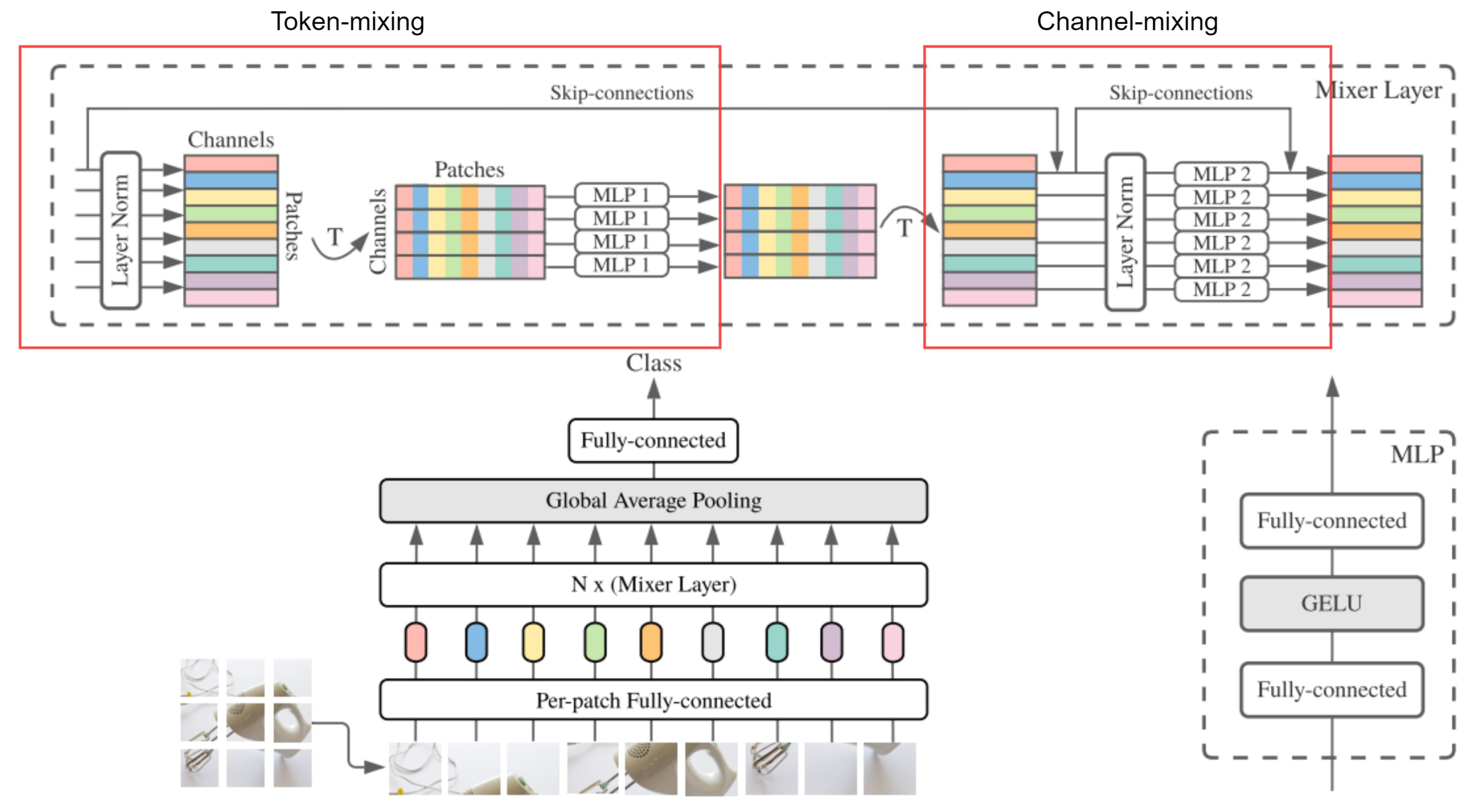
Figure 1 illustrates the MLP-Mixer architecture. The input is divided into unique patches which do not overlap. The patches are linearly projected into an embedding space. In contrast to the transformer and ViT, the input does not need positional embeddings, as the Mixer is sensitive to the position of the inputs in the token-mixing MLPs [
8]. The Mixer consists of two types of MLP layers, the token-mixing layer and the channel-mixing layer. The inspiration behind this is that modern vision neural architectures, according to [
8],
(1) mix their features at a given spatial location across channels and
(2) mix their features between different spatial locations. CNNs implement (1) with a convolution layer through the 1 x 1 convolution operation, and (2) using large kernels and by adding multiple convolution layers with pooling which decreases the input spatially. In attention-based models, both (1) and (2) are performed within each self-attention layer. The Mixer’s purpose is to separate per-location operations (1) and cross-location operations (2). These features are achieved through two layers, called "token-mixing" and "channel-mixing", representing the per-location and the cross-location operations, respectively.
Each unique patch has identical dimensions. The number of patches is calculated by dividing the input dimensions (H, W) by the patch resolution(P, P), . The sequence of non-overlapping patches is projected into an embedding space with dimension C, resulting in a matrix of dimensions SxC. The layers in the Mixer are all the same size and are made up of two MLP blocks each.
The first block is the token-mixing MLP; the input matrix is normalised and transposed to allow the data to mix across each patch. The MLP(MLP1) will act on each column of the input matrix, sharing its weights across the columns. The matrix is transposed back into its original form. The overall context of the input is obtained by feeding each patch’s data into the MLP. This token-mixing block essentially allows different patches in the same channel to communicate.
The second block is the channel-mixing MLP; this receives residual connections from its pre-normalised original input to prevent information from being lost during the training process. The result is normalised, and a different MLP(MLP2) performs the channel-mixing with a separate set of weights. The MLP acts on each input matrix row, and its weights are shared across the rows. A single patch’s MLP receives data from every channel, enabling communication between the information from various channels.
Each MLP block contains two feed-forward layers with a GELU [
35] activation function applied to each row of the input data. The Mixer layers are calculated in equation
1 (the layer index is not included) and the GELU function is demonstrated in equation
2.
It is intuitive to share the weights in each layer of the channel-mixing MLPs, as this offers positional invariance, a key characteristic of convolution layers in CNNs. However, it is less intuitive to share the weights across channels in the token-mixing MLPs. For instance, some CNNs use separable convolutions [
36], which apply convolutions to each channel independently of the other. However, these convolutions apply different filters to each channel, in contrast to the token-mixing MLPs, which use the same filter for all channels. Additionally, sharing weights in the token-mixing and channel-mixing layers prevents the Mixer from growing in size quickly when the number of patches,
S, or the dimensions of the embedding space,
C, increases, leading to substantial memory savings. Furthermore, the empirical performance of this model is unaffected by this characteristic.
4. Datasets
To evaluate the performance of the MLP-Mixer in classifying a variety of activities, three datasets are used for benchmarking.
4.1. Opportunity
The opportunity dataset [
10] contains complex labelled data collected from multiple body sensors. It consists of data from 4 subjects recorded in a daily living scenario designed to create multiple activities in a realistic manner. Each subject had six sets of data.
The opportunity dataset consists of all three types of human activities, recurrent, static, and spontaneous. The subjects wore a body jacket which contained five inertial measurement units (IMU), made up of a 3D accelerometer, gyroscope and magnetic sensor, two inertial sensors for both feet, and 12 wireless accelerometers sensors, which suffered from data loss due to their Bluetooth connection. In this dataset, only sensor data without packet loss was used. This included data from the inertial sensors on both feet and the accelerometer sensors on the back and upper limbs, resulting in each sample containing 77 dimensions of sensor data when combining all the sensor data together. The sensors recorded the data at a sampling rate of 30Hz. Mixer is trained, validated and tested on are similar to that in previous literature [
19,
37,
38,
39,
40,
41] for consistency and fair comparison. The Mixer was tested on ADL4 and AD5 from subjects 2 and 3, ADL2 from subject 1 was used as the validation set, and the rest of the ADLs and all the drill sessions were used for training the Mixer. The Opportunity dataset has multiple benchmark HAR tasks, including:
Opportunity gestures: This involves successfully classifying different gestures being performed by the subjects from both arm sensors. There are 18 different gesture classes.
Opportunity locomotion: This involves accurately classifying the locomotion of the subjects the full body sensors. There are five different locomotion classes.
4.2. PAMAP2
The PAMAP2 dataset [
12] contains complex labelled data collected from chest, hand and ankle sensors. This consisted of data recorded from nine subjects. Each subject followed a routine of 12 different actions and optionally performed an addition of 6 activities resulting in 18 recorded activities each, 19 if you include the null class.
The PAMAP2, similar to the Opportunity dataset, contains all three types of human activities. The nine subjects wore IMUs on their hands, ankles and chest. The IMU recorded multimodal data, which consisted of an accelerometer, gyroscope, heart rate, temperature and magnetic data. In total, the data contains 40 sensor recordings and 12 IMU orientation data points, resulting in each sample containing 52 dimensions of sensor data when combined. Each sensor sampled the data at a sampling rate of 100Hz, and the dataset was downsampled to approximately 33.3Hz to have a similar sampling rate to the opportunity dataset. There were missing data present in the dataset from the packet loss of the wireless sensors. To account for this, only the heart rate sensor was interpolated; afterwards, samples with missing values were excluded from the dataset. The parts of the dataset that are trained, tested and validated are identical to previous literature [
39,
42]. The Mixer was tested on subject 6 and validated on subject 5, and the rest were used for training; however, subject 9 was dropped due to significantly less sensor data compared to the rest of the subjects. Additionally, the orientation data points were not used as they were unimportant for this problem, leaving the dataset with a dimension of 40 features. To make the experiments performed on PAMAP2 comparable with previous literature, the optional activities and the null activities are excluded while training the Mixer, resulting in a total of 12 classes to be classified.
4.3. Daphnet Gait
The daphnet gait dataset [
11] contains labelled data collected from accelerometer sensors. It consists of data collected from 10 subjects who are affected with Parkinson’s Disease (PD). The subjects are instructed to carry out three types of tasks, walking in a straight line, walking while turning, and realistic ADL scenarios which involve tasks such as getting coffee. These tasks were designed to frequently induce gait freezing in the subjects. Freezing is a common symptom of PD, which causes difficulty starting movements, such as taking steps, for a short period of time [
19]. The goal of the dataset is to detect whether the subjects are freezing or doing the specified actions (walk, turn). This is a binary classification problem since the specified action are combined into one class,
No Freeze, and the "Null" class is excluded from the experiment.
Accelerometers were used to capture information about the subjects. They were placed on the chest, above the ankle and above the knee, resulting in each sample containing 9 dimensions of sensor data when combined. Each sensor sampled the data at a sampling rate of 64Hz, and the dataset was downsampled to 32Hz for temporal comparison with the other datasets. A fair comparison was maintained by splitting the dataset into training, validation, and testing sets identical to early literature [
19]. The Mixer was tested on data from subject 2, validated on subject 9 and trained using the rest of the information.
4.4. Sliding Windows
For the datasets to be trained and tested by the Mixer, a sliding window approach is used on the dataset. This splits the dataset into multiple sequences with the dimensions, (
X
), where
is the number of features in the dataset and
is the sliding window length. These 2D sequences, in the case of the Mixer, are treated as images. The length of the sliding window maintains a fixed length throughout each separate training process but varies across the different datasets and experiments. As mentioned in
Section 3.1, the Mixer takes an input image with dimensions (
H,
W) that is split into patches with identical dimensions (
P,
P). This requires the patch resolution,
P, to be fully divisible by both dimensions of the input. This limits the length of the sliding window to either be divisible by the number of features in the dataset or divisible by the patch resolution.
The Mixer outputs a prediction of the activity for every sliding window interval after observing it; however there would be multiple predictions in the sliding window instead of a single ground truth prediction. There are multiple methods around this [
42,
43], which involve using the prediction at the end of the sliding window, max-pooling all of the sequence predictions over time, or returning the most frequent predictions. The Mixer benefits from mixing its features at a given spatial location across channels and between different spatial locations. In addition, the token-mixing MLP provides a global context of the input to the model. Therefore using the most frequent predictions as the ground truth prediction is preferred to other methods since the Mixer learns context from the whole input. The details of the sliding window for each dataset are briefly described below, and the summary of their parameters is tabulated in
Table 1.
Opportunity: The dataset was fit into a sliding window with an interval of 2.57 seconds. This duration represents 77 samples, which makes the input dimensions identical, allowing the patch resolution to be a factor of 77. The dataset was normalised to account for the wide range of sensors used in the dataset. After preprocessing the data, there were no labels of "close drawer 2" activity in the test set (ADL4 and AD5 from subjects 2 and 3).
PAMAP2: Before downsampling, the dataset was fitted into a sliding window interval of 0.84 seconds, which corresponds to 84 samples. The "rope-jumping" activity in subject 6 had a very small number of samples. After preprocessing, there were no labels of this activity present in the test set (subject 6).
Daphnet Gait: Before downsampling, a sliding window interval of 2.1 seconds was used to fit the dataset; this interval corresponds to 126 samples. Daphnet Gait contains a lot of longer activities, so a wider sliding window interval was chosen to provide the Mixer with more information.
Large sliding windows were used to give the Mixer access to more information and enable the sequence to be divided into patches correctly and error-free. Smaller step sizes were used because the Mixer tends to overfit, giving it more training points and ensuring that there were enough data points for adequate testing on the various activities in each dataset.
4.5. Data Sampler and Generation
A class balance sampler was applied to the training dataset to give similar probability to the classes during training allowing the Mixer to learn from each class equally in the imbalanced datasets. The different samples are stored based on their labelled class. During each batch, the sampler accesses the training samples based on their weights. The samples are weighted based on the proportion of their class in the training dataset.
4.6. Patches
The MLP-Mixer requires a sequence of input patches. This layer converts the input sensor data into separate patches. The patch resolution has to be fully divisible by both the input height and width dimensions. The patch resolution differed between datasets and the resolution for each dataset is tabulated in
Table 2. This was implemented using a strided Conv2D layer in Pytorch. A strided Conv2D layer produces the same results as the per-patch fully-connected layer used in [
8]. This layer reshapes the input from (number of samples, number of channels, input height, input width) to (number of samples, number of patches, patch embedding dimensionality).
5. Experimental Setup
The Mixer was trained using the Adam optimiser with the cross-entropy loss as the criterion and hyperparameters = 0.9, = 0.999. The Mixer has a tendency to overfit, so a weight decay of 1e-3 was used. The gradient clipping at the global norm was set to 1, and the batch size for the training and testing dataset was 64. A learning rate scheduler was used, and the learning rate was set to 0.01. For the first 500 steps, the learning rate scheduler used a linear warm-up rate. Then, until the training was finished, it used a cosine decay.
The specifications of the Mixer architecture used to produce the main results in
Section 6 is tabulated in
Table 2. The experiments were run five times with the best specifications, and the mean of the results was taken.
5.1. Ablation Study
The Mixer is ablated to compare the importance of different design choices of the MLP-Mixer in HAR. The different design choices involve the architecture of the Mixer (token-mixing MLP, channel-mixing MLP) and the RGB embedding layer. The macro score is used in the ablation study to assess the model. This prevents high evaluation scores by simply choosing the majority class in imbalanced datasets and provides accurate insight into the model’s learning capabilities across class activities.
The MLP-Mixer without RGB Embedding: The Mixer saw a slight decrease in performance, which meant that this layer had some contribution to the Mixer’s learning capabilities. This allows the sensor data to simulate the RGB channels in images. This produces three sets of features for the Mixer to project into its embedding space instead of a single set of features from the single sensor channel. The results are tabulated in
Table 3.
The MLP-Mixer without the Token-Mixing MLPs: The model had a significant decrease in performance in all the datasets without the token-mixing MLPs. The Mixer uses token-mixing to learn global context from the input and communicate information between patches; without this layer, the Mixer can not effectively capture the spatial and temporal information of the activities in the datasets. The results tabulated in
Table 3 indicate the Mixer loses its capabilities to learn relevant features of the dataset; hence it can be concluded that the token-mixing MLP is necessary for the Mixer to perform well in HAR benchmark datasets.
The MLP-Mixer without the Channel-Mixing MLPs: The channel-mixing MLPs allow the model to communicate between channels, essentially acting as a 1x1 convolution. It enables the Mixer to detect features between channels, and without it, only spatial information between the various patches will be learned. The results tabulated in
Table 3 showcase substantial performance loss which indicates that the channel-mixing MLP is important for HAR. However, the performance loss is lower compared to the performance loss in the absence of the token-mixing MLPs. This indicates that the channel-mixing MLP is a supplement to the token-mixing MLP, communicating the information learned from the token-mixing layer across channels rather than capturing core features needed for accurate prediction in HAR.
6. Results
The Mixer is compared with the following state-of-the-art architectures:
Ensemble LSTMs [37]: combines multiple LSTMs using ensemble techniques to produce a single LSTM.
CNN-BiGRU [44]: CNN connected with a biGRU.
AttenSense [25]: a CNN and GRU are combined using an attention mechanism to learn spatial and temporal patterns.
Multi-Agent Attention [45]: combines multi-agent collaboration with attention-based selection.
DeepConvLSTM [42]: combines an LSTM to learn temporal information with a CNN to learn spatial features.
BLSTM-RNN [38]: a bi-LSTM, with its weights and activation functions binarized.
Triple Attention [46]: a ResNet, using a triple-attention mechanism.
Self-Attention [47]: a self-attention-based model without any recurrent architectures.
CNN [19]: a CNN with three layers and max pooling.
b-LSTM-S [19]: bidirectional LSTM that uses future training data.
Table 4 shows the performance comparison between the Mixer and existing state-of-the-art literature.
Table 4 shows that the MLP-Mixer performs better than previous techniques in the Opportunity Locomotion, PAMAP2, and the Daphnet Gait datasets. Despite the model’s shortcomings in the Opportunity Gestures dataset, it is still competitive with most of the previously developed methods. Sliding window techniques were used in all the previous techniques, with only the sliding window lengths and overlaps differing. Although the Mixer beats the previous techniques in Opportunity Locomotion, most previous work that used the Opportunity dataset for performance evaluation only focused on the gesture classification task while disregarding the locomotion task.
The sliding window lengths used were similar to or larger than previous techniques, allowing the model to capture more information from each interval. Therefore, it can be concluded that the MLP mixer model can learn the spatial and temporal dynamics of the sensor data more effectively than the previous models. The Mixer performs better than existing attention and convolution-based models in PAMAP2. The macro-score of the Mixer is slightly higher(0.97) than the triple-attention model [
46] (0.96) and significantly higher than the best convolution-based model [
19] (0.937), it performed better than the state-of-the-art by 1%. In the daphnet-gait dataset the model also performed better than convolution and recurrent models, producing a macro-score of 0.842 compared to 0.741. It performed better than the state-of-the-art by 10.1%. However, existing literature using the Daphnet Gait focus more on future prediction [
48,
49,
50] instead of recognition and use different evaluation metrics, therefore cannot be directly compared to the Mixer. In the opportunity gestures, the Mixer remains competitive but does not perform better than the b-LSTM-S, the opportunity dataset was particularly challenging for the MLP-Mixer, due to shorter activities combined with a larger sliding window necessary for the image to be split into patches. As a result, there were several activities in the training sliding window, making it more difficult for the Mixer to learn and harder for it to predict activities in the test sliding window. The b-LSTM-S performed 1.7% better than the Mixer in this dataset.
7. Discussion
Convolutions capture the spatial information in a local area of the data. However, they are not effective at learning long-term dependencies (temporal data) [
27], unlike recurrent networks, which specialise in long-term dependencies. The self-attention mechanism learns the entire context of input patches. Additionally, it learns what to pay attention to based on its weights [
47], allowing it to learn the relationship between the sensors and the different activities. The token-mixing MLPs can be considered a convolution layer that captures information about the entire input. It combines spatial information from a single channel and distributes channel weights to increase efficiency, which allows the Mixer to perform better than previous techniques when an adequate amount of data is provided and the invariant features of the input are coherent.
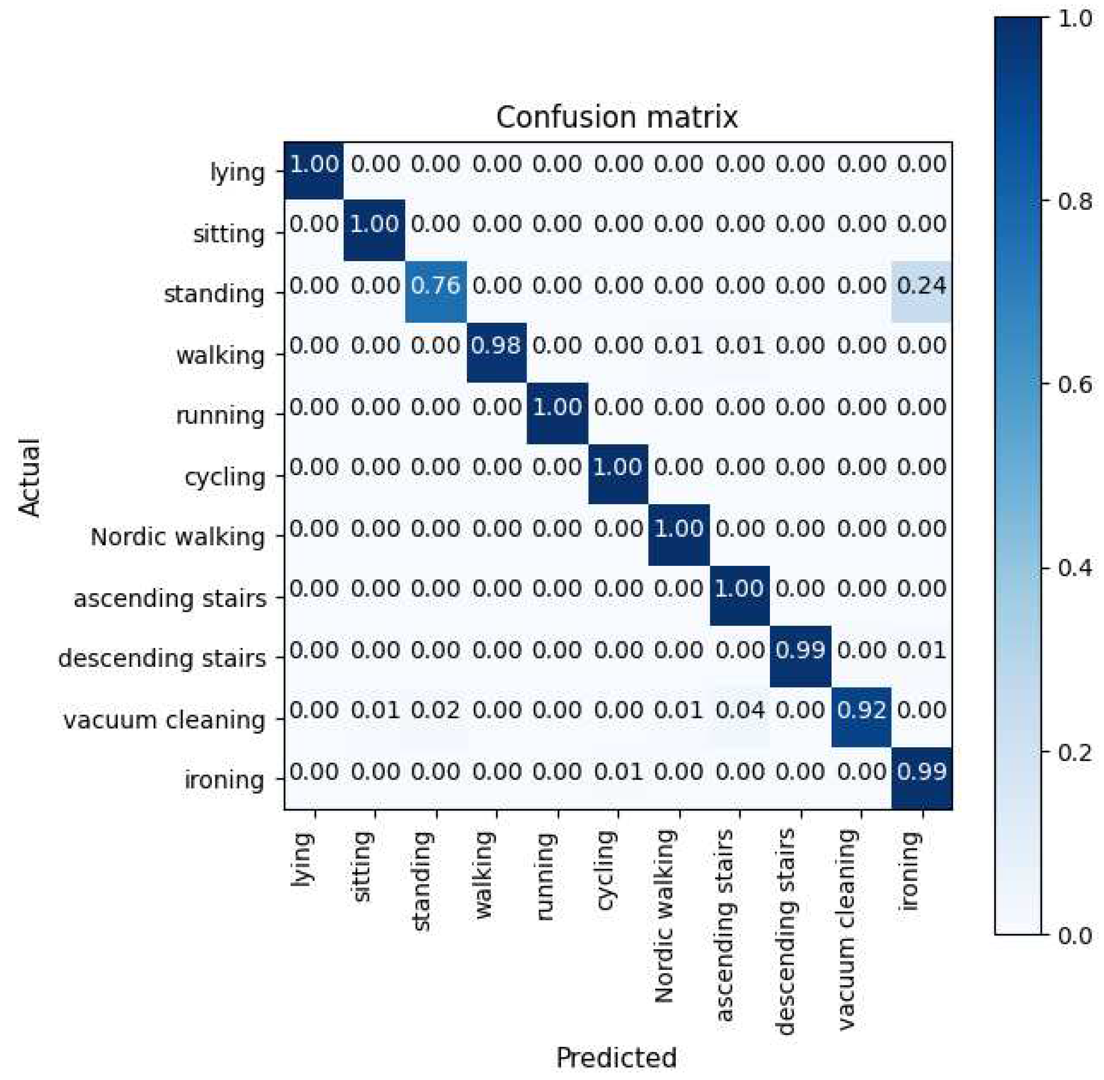
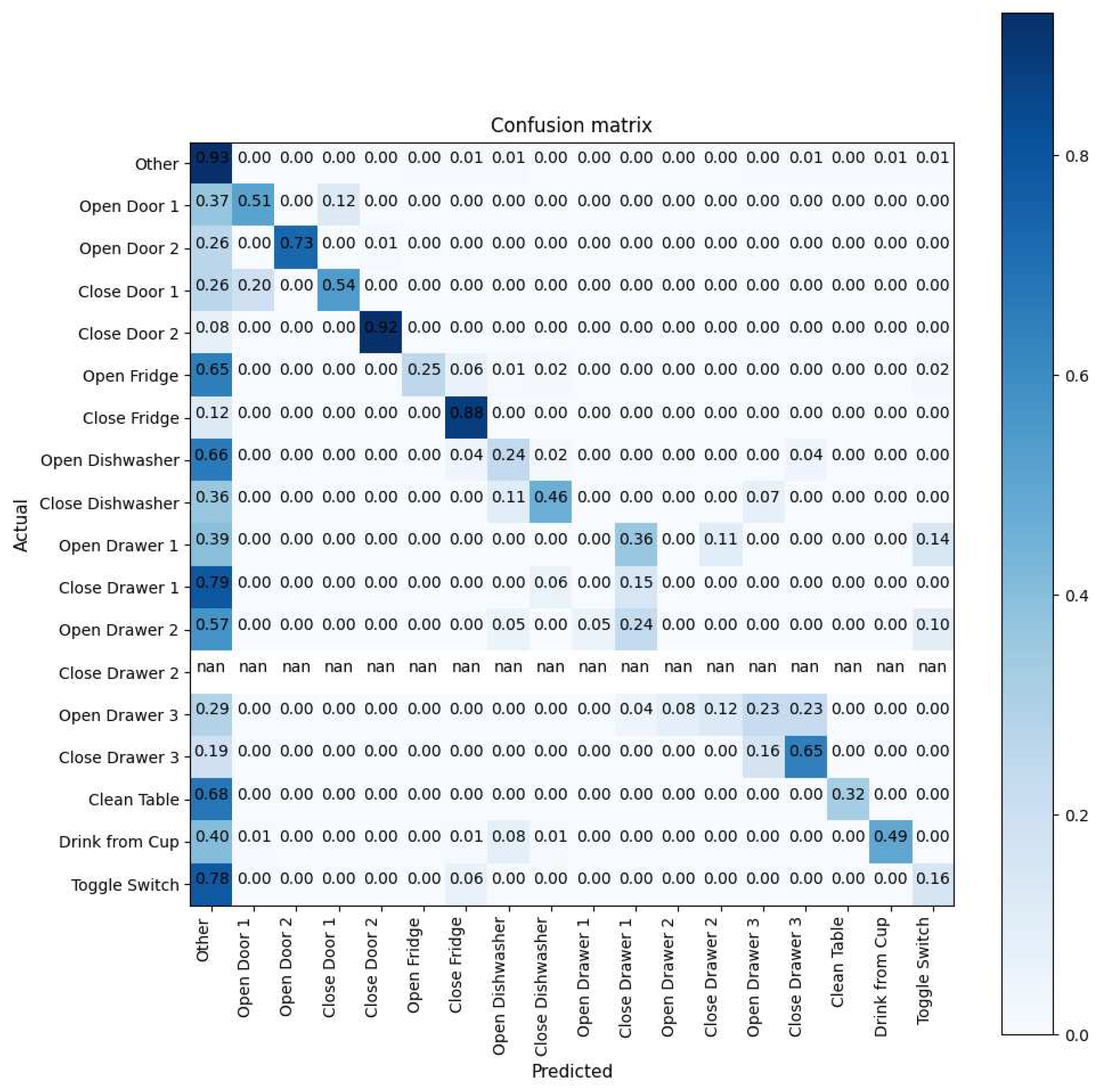
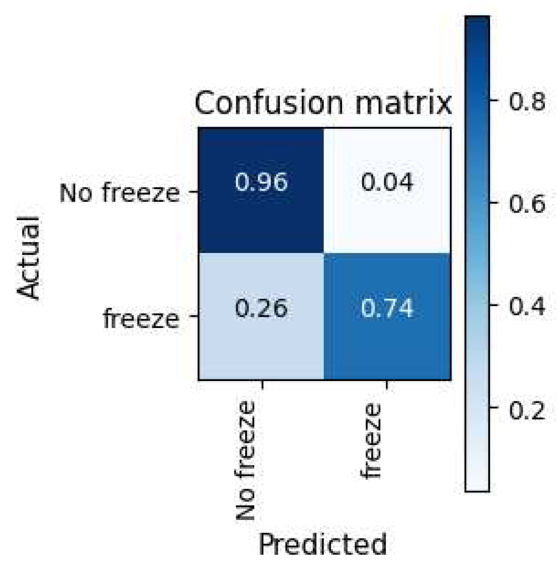
The normalised confusion matrices of the PAMAP2, Opportunity and Daphnet datasets are illustrated in
Figure 2,
Figure 3 and
Figure 4, respectively. The model’s ability to distinguish between activities in the PAMAP2 confusion matrix showed that it had learned various spatial and temporal characteristics of each activity. The model did have some trouble distinguishing between the "ironing" and "standing" activities; this is probably because the sensor data for these actions are similar in the chest and ankle regions but only slightly different in the hand regions. With further inspection, standing consisted of talking while gesticulating, further validating the possibility of similarities in the hand sensors. Furthermore, The model had little trouble differentiating "walking", "vacuum cleaning", and "descending stairs" activities; this is understandable since it mistook these activities for similar ones.
It was more difficult for the model to distinguish between different activities in the Opportunity dataset. Because there were significantly more samples of Null activities than any other activity, the Opportunity confusion matrix,
Figure 3, shows that the model frequently mistook activities for being unrelated. Furthermore, because the activities were short, the model had a more challenging time figuring out where a given activity began and ended in the sliding window. The confusion matrix demonstrates that the model was could pick up on some of the "open door 2" and "close fridge" activity characteristics. However, the model did not successfully capture features of "open drawer 1" and mistook this activity for "close drawer 1". Further investigation revealed that the activity—which consisted of opening and closing the drawer—took place in a single sequence, suggesting that the model could not determine when the activity began and, therefore, could not correctly distinguish between the two.
There was a significant imbalance between the two activities in the Daphnet Gait dataset, much like in the opportunity dataset. As shown in
Figure 4, the Mixer was trained on an adequate sample size for the majority class,” No freeze,” allowing it to learn when the participants were not freezing correctly. However, in the minority case, there was insufficient data from the Mixer to properly learn relevant features, resulting in the Mixer incorrectly classifying the participants as not freezing 26% of the time.
8. Performance of Sliding Window Parameters
Each dataset contains a different range of activity lengths and repetition rates. The sliding window length has a significant impact depending on how long the activities are in the dataset. The sliding window’s parameters were altered to study its effect on the Mixer performance. The model’s parameters were fixed, and the step size was constant instead of using an overlap percentage of the window length to prevent the number of samples from affecting the results. Small window intervals contain insufficient data for the Mixer to learn from and make decisions. On the other hand, if the sliding window interval is large relative to the activities in the window, it allows information from multiple activities to be present in a single sliding window, making it harder for the Mixer to determine which activity the sliding window represents among the multiple activities.
Performance generally improves with increasing overlap, but as there are more samples to train and test, the computational complexity of training the Mixer also rises. In contrast, little to no overlap significantly reduces the sample size, particularly for larger sliding window sizes, which causes the Mixer to over-fit on the dataset.
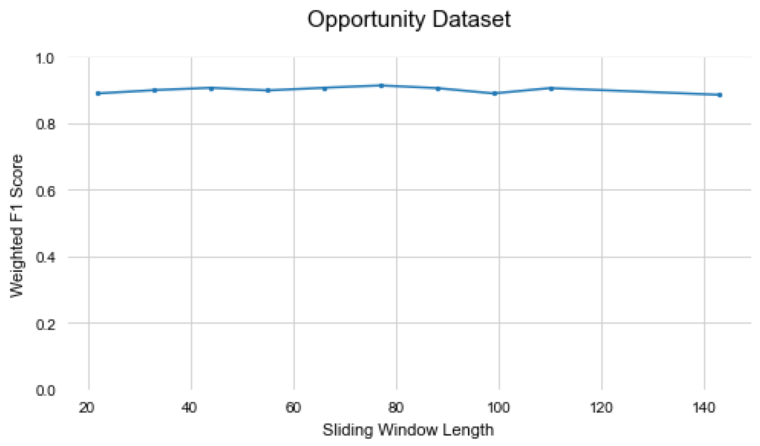
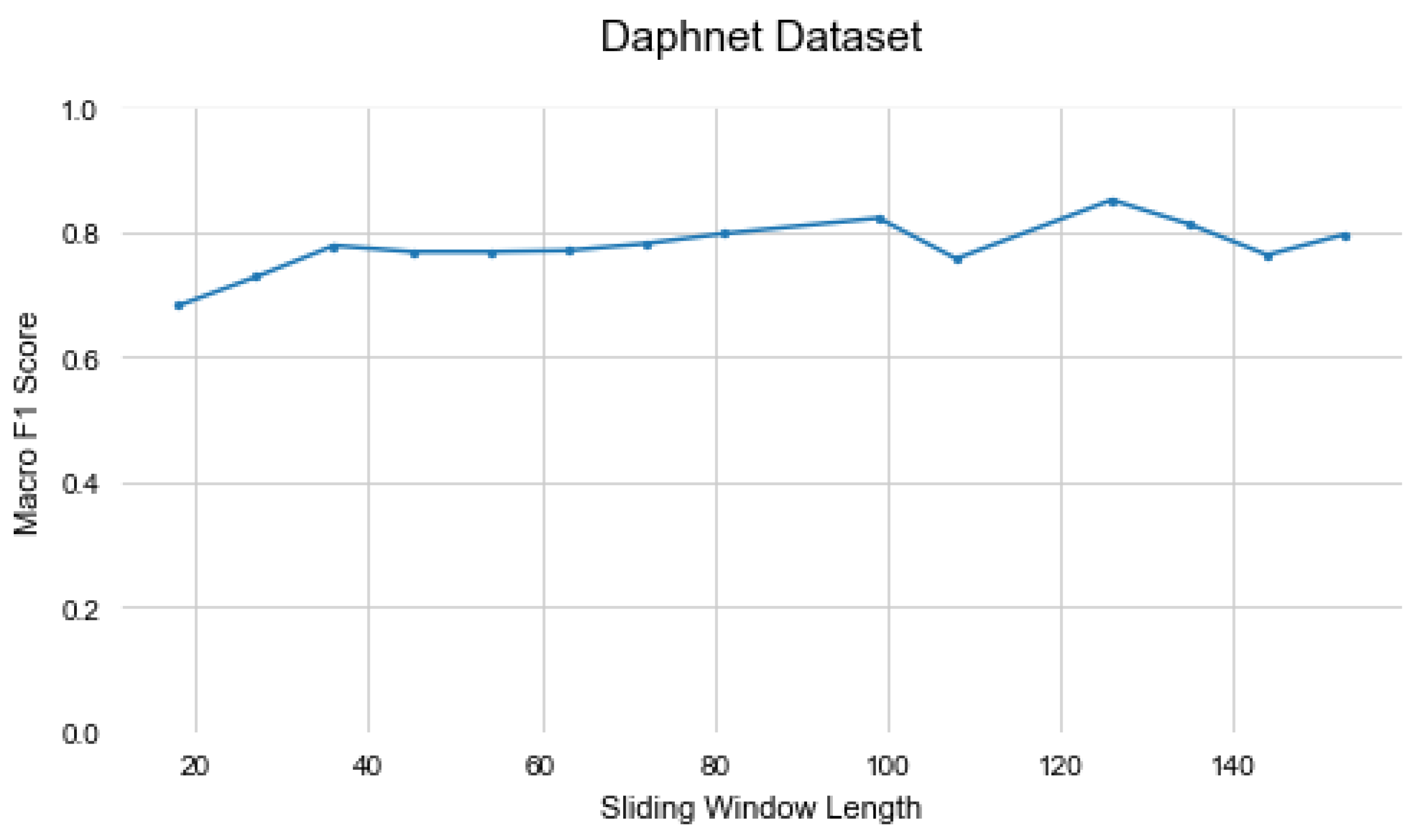
Figure 5,
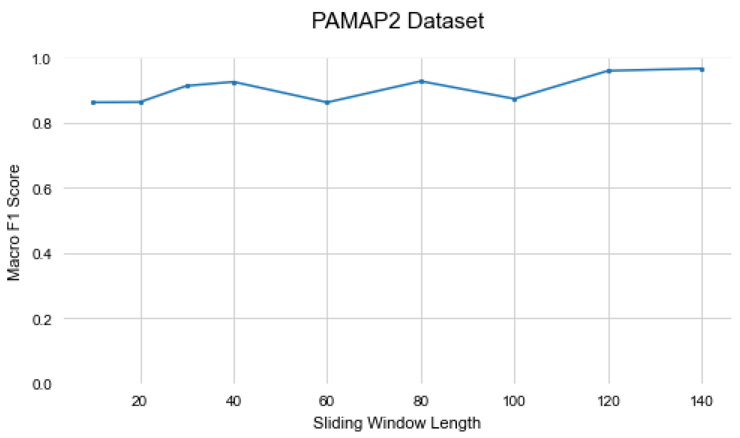
Figure 6 and
Figure 7 illustrate the changes in the Mixer’s performance when the sliding window length is changed. In datasets with more extended activities, such as PAMAP2 and Daphnet, larger sliding windows increase the model’s capability to learn by providing more information. On the other hand, in the Opportunity dataset, which contains shorter activities, the model’s performance decreases with larger window lengths. The sliding window figures indicate that the sliding window has a slight effect on the Mixer’s performance, but overall the model is not sensitive to the sliding window length.
9. Weight Visualisation
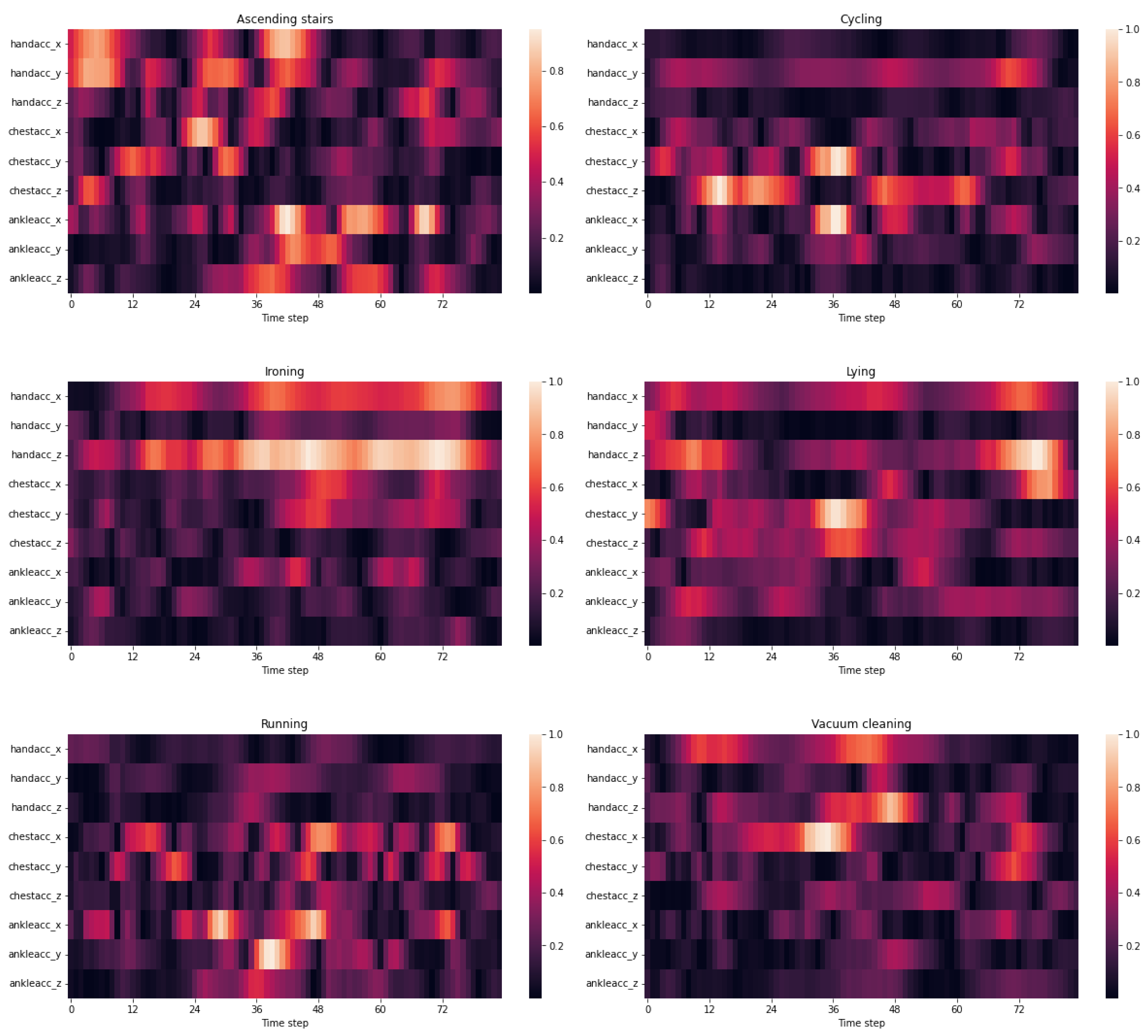
The models’ weights are visualised to provide insight into which sensors the model considers necessary for different activities. This experiment aims to confirm that the Mixer is capturing relevant features and to offer some interpretation of how the Mixer categorises the activities. The analysis is performed on the PAMAP2 dataset to showcase various simple and complex activities. Six different activities and their associated weights are illustrated in
Figure 8.
Figure 8 shows how the Mixer associates various sensors with various activities. The Mixer not only learns which sensors are crucial but also when they are crucial as the emphasis of sensors changes throughout the sliding window. For example, in ascending stairs, the hand(X, Y), chest(X), and ankle sensors have essential features that the Mixer emphasises, typical when climbing a staircase with handrails. Cycling focuses on the hand(Y) sensor, most likely for steering, and the chest and ankle sensors, likely for pedalling. The Mixer prioritises the hand’s (X, Z) sensors when ironing, as expected. While lying down, the Mixer considered all sensors important, except for the ankle (Z) and hand (Y), which is to be expected given that the participants had complete freedom to change their lying positions. Finally, the Mixer values the hand (X, Z) and chest (X) sensors for vacuum cleaning and the ankles (X, Y) and chest (X) sensors for running activities, which is consistent with common sense. This analysis concludes that the Mixer is successfully learning the spatial and temporal characteristics of the various activities because the weight assignments for these activities are understandable and in tune with common sense.
10. Conclusions
In this paper, the MLP-Mixer performance is investigated for HAR. The Mixer does not use convolutions or self-attention mechanisms and instead relies solely on MLPs. It uses token-mixing and channel mixing layers to communicate between patches and channels, learning the global context of the input and enabling excellent spatial and temporal pattern recognition in HAR. Experiments were performed on three popular HAR datasets, Opportunity, PAMAP2 and Daphnet Gait. The Mixer was assessed using sliding windows on the dataset. This paper demonstrates that pure-MLP architectures can compete with convolutional and attention-based architectures in terms of HAR viability and performance. We demonstrate that the MLP-Mixer outperforms current state-of-the-art models in the test benchmarks for all datasets except for Opportunity Gestures. It performs 10.1% better in the Daphnet Gait dataset, 1% better in the PAMAP2 dataset and 0.5% in the Opportunity Locomotion dataset. The Mixer was outperformed in the Opportunity Gestures; however it remained competitive with the state-of-the-art results. To the best of my knowledge vision-based MLP architectures have not been applied to HAR tasks. It is interesting to see the performance of a pure-MLP architecture, outperform and remain competitive with state-of-the-art models in HAR.
References
- Parker, S.J.; Strath, S.J.; Swartz, A.M. Physical Activity Measurement in Older Adults: Relationships With Mental Health. Journal of aging and physical activity 2008, 16, 369–380. [Google Scholar] [CrossRef] [PubMed]
- Kranz, M.; Möller, A.; Hammerla, N.; Diewald, S.; Plötz, T.; Olivier, P.; Roalter, L. The mobile fitness coach: Towards individualized skill assessment using personalized mobile devices. Pervasive and Mobile Computing 2013, 9, 203–215. [Google Scholar] [CrossRef]
- Patel, S.; Park, H.S.; Bonato, P.; Chan, L.; Rodgers, M. A Review of Wearable Sensors and Systems with Application in Rehabilitation. Journal of neuroengineering and rehabilitation 2012, 9, 21. [Google Scholar] [CrossRef] [PubMed]
- Cedillo, P.; Sanchez-Zhunio, C.; Bermeo, A.; Campos, K. A Systematic Literature Review on Devices and Systems for Ambient Assisted Living: Solutions and Trends from Different User Perspectives. 2018. [CrossRef]
- De Leonardis, G.; Rosati, S.; Balestra, G.; Agostini, V.; Panero, E.; Gastaldi, L.; Knaflitz, M. Human Activity Recognition by Wearable Sensors : Comparison of different classifiers for real-time applications. 2018 IEEE International Symposium on Medical Measurements and Applications (MeMeA), 2018, pp. 1–6. [CrossRef]
- Park, S.; Jayaraman, S. Enhancing the quality of life through wearable technology. IEEE Engineering in Medicine and Biology Magazine 2003, 22, 41–48. [Google Scholar] [CrossRef] [PubMed]
- Lara, O.D.; Labrador, M.A. A Survey on Human Activity Recognition using Wearable Sensors. IEEE Communications Surveys and Tutorials 2013, 15, 1192–1209. [Google Scholar] [CrossRef]
- Tolstikhin, I.O.; Houlsby, N.; Kolesnikov, A.; Beyer, L.; Zhai, X.; Unterthiner, T.; Yung, J.; Steiner, A.; Keysers, D.; Uszkoreit, J.; Lucic, M.; Dosovitskiy, A. MLP-Mixer: An all-MLP Architecture for Vision. CoRR, 2021. [Google Scholar]
- Le, V.T.; Tran-Trung, K.; Truong, V. A Comprehensive Review of Recent Deep Learning Techniques for Human Activity Recognition. Computational Intelligence and Neuroscience 2022, 2022. [Google Scholar] [CrossRef] [PubMed]
- Roggen, D.; Calatroni, A.; Rossi, M.; Holleczek, T.; Förster, K.; Tröster, G.; Lukowicz, P.; Bannach, D.; Pirkl, G.; Ferscha, A.; Doppler, J.; Holzmann, C.; Kurz, M.; Holl, G.; Chavarriaga, R.; Sagha, H.; Bayati, H.; Creatura, M.; Millàn, J.d.R. Collecting complex activity datasets in highly rich networked sensor environments. 2010 Seventh International Conference on Networked Sensing Systems (INSS), 2010, pp. 233–240. [CrossRef]
- Bächlin, M.; Plotnik, M.; Roggen, D.; Maidan, I.; Hausdorff, J.; Giladi, N.; Troster, G. Wearable Assistant for Parkinson’s Disease Patients With the Freezing of Gait Symptom. Information Technology in Biomedicine, IEEE Transactions on 2010, 14, 436–446. [Google Scholar] [CrossRef] [PubMed]
- Reiss, A.; Stricker, D. Introducing a New Benchmarked Dataset for Activity Monitoring. 2012 16th International Symposium on Wearable Computers, 2012, pp. 108–109. [CrossRef]
- Zappi, P.; Lombriser, C.; Stiefmeier, T.; Farella, E.; Roggen, D.; Benini, L.; Tröster, G. Activity Recognition from On-Body Sensors: Accuracy-Power Trade-Off by Dynamic Sensor Selection. Wireless Sensor Networks; Verdone, R., Ed.; Springer Berlin Heidelberg: Berlin, Heidelberg, 2008; pp. 17–33. [Google Scholar]
- Weiss, G.M.; Yoneda, K.; Hayajneh, T. Smartphone and Smartwatch-Based Biometrics Using Activities of Daily Living. IEEE Access 2019, 7, 133190–133202. [Google Scholar] [CrossRef]
- Banos, O.; García, R.; Holgado-Terriza, J.; Damas, M.; Pomares, H.; Rojas, I.; Saez, A.; Villalonga, C. mHealthDroid: A Novel Framework for Agile Development of Mobile Health Applications. 2014, Vol. 8868, pp. 91–98. [CrossRef]
- Banos, O.; Villalonga, C.; García, R.; Saez, A.; Damas, M.; Holgado-Terriza, J.; Lee, S.; Pomares, H.; Rojas, I. Design, implementation and validation of a novel open framework for agile development of mobile health applications. BioMedical Engineering OnLine 2015, 14, S6. [Google Scholar] [CrossRef] [PubMed]
- Anguita, D.; Ghio, A.; Oneto, L.; Parra, X.; Reyes-Ortiz, J.L. A Public Domain Dataset for Human Activity Recognition using Smartphones. ESANN, 2013.
- Zeng, M.; Nguyen, L.T.; Yu, B.; Mengshoel, O.J.; Zhu, J.; Wu, P.; Zhang, J. Convolutional Neural Networks for human activity recognition using mobile sensors. 6th International Conference on Mobile Computing, Applications and Services, 2014, pp. 197–205. [CrossRef]
- Hammerla, N.Y.; Halloran, S.; Ploetz, T. Deep, Convolutional, and Recurrent Models for Human Activity Recognition using Wearables. CoRR, 2016. [Google Scholar]
- He, K.; Zhang, X.; Ren, S.; Sun, J. Deep Residual Learning for Image Recognition. CoRR, 1512. [Google Scholar]
- Tang, Y.; Teng, Q.; Zhang, L.; Min, F.; He, J. Layer-Wise Training Convolutional Neural Networks With Smaller Filters for Human Activity Recognition Using Wearable Sensors. IEEE Sensors Journal 2021, 21, 581–592. [Google Scholar] [CrossRef]
- Yang, Z.; Wang, Y.; Liu, C.; Chen, H.; Xu, C.; Shi, B.; Xu, C.; Xu, C. LegoNet: Efficient Convolutional Neural Networks with Lego Filters. Proceedings of the 36th International Conference on Machine Learning; Chaudhuri, K.; Salakhutdinov, R., Eds. PMLR, 2019, Vol. 97, Proceedings of Machine Learning Research, pp. 7005–7014.
- Murad, A.; Pyun, J.Y. Deep Recurrent Neural Networks for Human Activity Recognition. Sensors 2017, 17. [Google Scholar] [CrossRef] [PubMed]
- Nafea, O.; Abdul, W.; Muhammad, G.; Alsulaiman, M. Sensor-Based Human Activity Recognition with Spatio-Temporal Deep Learning. Sensors 2021, 21. [Google Scholar] [CrossRef] [PubMed]
- Ma, H.; Li, W.; Zhang, X.; Gao, S.; Lu, S. AttnSense: Multi-level Attention Mechanism For Multimodal Human Activity Recognition. Proceedings of the Twenty-Eighth International Joint Conference on Artificial Intelligence, IJCAI-19. International Joint Conferences on Artificial Intelligence Organization, 2019, pp. 3109–3115. [CrossRef]
- DanHAR: Dual Attention Network for multimodal human activity recognition using wearable sensors. Applied Soft Computing 2021, 111, 107728. [CrossRef]
- Liu, R.; Li, Y.; Tao, L.; Liang, D.; Zheng, H.T. Are we ready for a new paradigm shift? A survey on visual deep MLP. Patterns 2022, 3, 100520. [Google Scholar] [CrossRef] [PubMed]
- Liu, H.; Dai, Z.; So, D.R.; Le, Q.V. Pay Attention to MLPs. CoRR, 2021. [Google Scholar]
- Devlin, J.; Chang, M.; Lee, K.; Toutanova, K. BERT: Pre-training of Deep Bidirectional Transformers for Language Understanding. CoRR, 2018. [Google Scholar]
- Dosovitskiy, A.; Beyer, L.; Kolesnikov, A.; Weissenborn, D.; Zhai, X.; Unterthiner, T.; Dehghani, M.; Minderer, M.; Heigold, G.; Gelly, S.; Uszkoreit, J.; Houlsby, N. An Image is Worth 16x16 Words: Transformers for Image Recognition at Scale. CoRR, 2020. [Google Scholar]
- Yu, T.; Li, X.; Cai, Y.; Sun, M.; Li, P. S2-MLP: Spatial-Shift MLP Architecture for Vision. 2022 IEEE/CVF Winter Conference on Applications of Computer Vision (WACV), 2022, pp. 3615–3624. [CrossRef]
- Wei, G.; Zhang, Z.; Lan, C.; Lu, Y.; Chen, Z. ActiveMLP: An MLP-like Architecture with Active Token Mixer, 2022. [CrossRef]
- Tang, Y.; Han, K.; Guo, J.; Xu, C.; Li, Y.; Xu, C.; Wang, Y. An Image Patch is a Wave: Phase-Aware Vision MLP. CoRR, 2021. [Google Scholar]
- Wang, Z.; Jiang, W.; Zhu, Y.; Yuan, L.; Song, Y.; Liu, W. DynaMixer: A Vision MLP Architecture with Dynamic Mixing. CoRR, 2022. [Google Scholar]
- Hendrycks, D.; Gimpel, K. Bridging Nonlinearities and Stochastic Regularizers with Gaussian Error Linear Units. CoRR, 2016. [Google Scholar]
- Chollet, F. Xception: Deep Learning with Depthwise Separable Convolutions. CoRR, 2016. [Google Scholar]
- Guan, Y.; Ploetz, T. Ensembles of Deep LSTM Learners for Activity Recognition using Wearables. CoRR, 2017. [Google Scholar]
- Edel, M.; Köppe, E. Binarized-BLSTM-RNN based Human Activity Recognition. 2016 International Conference on Indoor Positioning and Indoor Navigation (IPIN), 2016, pp. 1–7. [CrossRef]
- Moya Rueda, F.; Grzeszick, R.; Fink, G.A.; Feldhorst, S.; Ten Hompel, M. Convolutional Neural Networks for Human Activity Recognition Using Body-Worn Sensors. Informatics 2018, 5. [Google Scholar] [CrossRef]
- Bock, M.; Hölzemann, A.; Moeller, M.; Laerhoven, K.V. Improving Deep Learning for HAR with shallow LSTMs. CoRR, 2021. [Google Scholar]
- Bock, M.; Hoelzemann, A.; Moeller, M.; Van Laerhoven, K. Improving Deep Learning for HAR with shallow LSTMs, 2021. [CrossRef]
- Ordóñez, F.J.; Roggen, D. Deep Convolutional and LSTM Recurrent Neural Networks for Multimodal Wearable Activity Recognition. Sensors 2016, 16. [Google Scholar] [CrossRef] [PubMed]
- Ng, J.Y.H.; Hausknecht, M.; Vijayanarasimhan, S.; Vinyals, O.; Monga, R.; Toderici, G. D: Short Snippets, 2015; arXiv:cs.CV/1503.08909].
- Mekruksavanich, S.; Jitpattanakul, A. Deep Convolutional Neural Network with RNNs for Complex Activity Recognition Using Wrist-Worn Wearable Sensor Data. Electronics 2021, 10. [Google Scholar] [CrossRef]
- Chen, K.; Yao, L.; Zhang, D.; Guo, B.; Yu, Z. Multi-agent Attentional Activity Recognition. CoRR, 2019. [Google Scholar]
- Tang, Y.; Zhang, L.; Teng, Q.; Min, F.; Song, A. Triple Cross-Domain Attention on Human Activity Recognition Using Wearable Sensors. IEEE Transactions on Emerging Topics in Computational Intelligence 2022, pp. 1–10. [CrossRef]
- Mahmud, S.; Tonmoy, M.T.H.; Bhaumik, K.K.; Rahman, A.K.M.M.; Amin, M.A.; Shoyaib, M.; Khan, M.A.H.; Ali, A.A. Human Activity Recognition from Wearable Sensor Data Using Self-Attention. CoRR, 2020. [Google Scholar]
- Li, B.; Yao, Z.; Wang, J.; Wang, S.; Yang, X.; Sun, Y. Improved Deep Learning Technique to Detect Freezing of Gait in Parkinson’s Disease Based on Wearable Sensors. Electronics 2020, 9, 1919. [Google Scholar] [CrossRef]
- Thu, N.T.H.; Han, D.S. Freezing of Gait Detection Using Discrete Wavelet Transform and Hybrid Deep Learning Architecture. 2021 Twelfth International Conference on Ubiquitous and Future Networks (ICUFN), 2021, pp. 448–451. [CrossRef]
- El-ziaat, H.; El-Bendary, N.; Moawad, R. A Hybrid Deep Learning Approach for Freezing of Gait Prediction in Patients with Parkinson’s Disease. International Journal of Advanced Computer Science and Applications 2022, 13. [Google Scholar] [CrossRef]
|
Disclaimer/Publisher’s Note: The statements, opinions and data contained in all publications are solely those of the individual author(s) and contributor(s) and not of MDPI and/or the editor(s). MDPI and/or the editor(s) disclaim responsibility for any injury to people or property resulting from any ideas, methods, instructions or products referred to in the content. |
© 2020 by the authors. Licensee MDPI, Basel, Switzerland. This article is an open access article distributed under the terms and conditions of the Creative Commons Attribution (CC BY) license (https://creativecommons.org/licenses/by/4.0/).
