Preprint
Article

Combination of Physics-Informed Neural Networks and Single-Relaxation-Time Lattice Boltzmann Method for Solving Inverse Problems in Fluid Mechanics

Altmetrics

Downloads

167

Views

88

Comments

0

A peer-reviewed article of this preprint also exists.

This version is not peer-reviewed

Submitted:

08 September 2023

Posted:

11 September 2023

You are already at the latest version

Alerts
Abstract
The Physics-Informed Neural Networks (PINNs) improve the efficiency of data utilization by combining physical principles with neural network algorithms and ensure that the predictions are consistent and stable with the physical laws. PINNs opens up a new approach to address inverse problems in fluid mechanics. Based on the single-relaxation-time lattice Boltzmann method (SRT-LBM) with the Bhatnagar-Gross-Krook (BGK) collision operator, the PINN-SRT-LBM model is proposed in this paper for solving the inverse problem in fluid mechanics. The PINN-SRT-LBM model consists of three components. The first component involves a deep neural network that predicts the equilibrium control equations in different discrete velocity directions within SRT-LBM. The second component employs another deep neural network to predict non-equilibrium control equations, enabling inference of the fluid's non-equilibrium characteristics. The third component, a physics informed function translates the outputs of the first two networks into physical infor-mation. By minimizing the residuals of the physical partial differential equations (PDEs), the physics informed function infers relevant macroscopic quantities of the flow. The model evolves two sub-models applicable to different dimensions, named PINN-SRT-LBM-I and PINN-SRT-LBM-II models according to the construction of the physical informed function. The innovation of this work is the introduction of SRT-LBM and discrete velocity models as physical drivers into the neural network through the interpretation function. Therefore, PINN-SRT-LBM allows the neural network to handle inverse problems of various dimensions and focus on problem-specific solving. Experimental results confirm the accurate prediction of flow infor-mation at different Reynolds numbers within the computational domain. Relying on the PINN-SRT-LBM models, inverse problems in fluid mechanics can be solved efficiently.
Keywords: 
Subject: Computer Science and Mathematics  -   Mathematics

1. Introduction

Machine learning has experienced rapid growth over the past few decades, bringing forth fresh opportunities across multiple application domains. These new opportunities have a significant impact on the fields of science and engineering and provide chances for paradigm shifts. Machine learning has introduced novel possibilities for modeling, predicting, and solving inverse problems related to fluid mechanics research [1].
Deep learning, as one of the most crucial branches of machine learning, has achieved remarkable success across various application domains. Particularly, deep learning has demonstrated significant accomplishments in areas such as computer vision, natural language processing, and speech recognition [2,3,4]. Deep learning algorithms can handle large-scale intricate data, extract advanced features, and attain exceptional performance in various tasks[5], such as image classification, object detection, semantic segmentation, and machine translation [6,7,8,9]. Common DNN (Deep Neural Network) models encompass a variety of architectures, including the Multilayer Perceptron (MLP) [10],Convolutional Neural Network (CNN) [11] and Recurrent Neural Network (RNN) [12].
Over the past several decades, CFD has undergone significant development in numerical simulations of both incompressible and compressible flows. Great progress has been achieved in CFD through finite difference method [13], finite volume method [14], finite element method [15], and spectral method [16]. CFD has made significant advancements in the domains of microscale and mesoscale methods. For instance, molecular dynamics [17], cellular automata[18], lattice Boltzmann methods (LBM) [19], and others have contributed to these developments. As a mesoscopic CFD method, LBM is based on the evolution of statistical distributions on the lattice. LBM has achieved considerable success in simulating fluid flow and associated transport phenomena [20]. In particular, LBM is able to handle a wide variety of boundary conditions and complex geometries with a simple program structure and a high degree of parallelism [21]. The most commonly used model in LBM is the single relaxation time LBM (SRT-LBM). Despite some limitations of the SRT-LBM, such as the challenges of flow simulation at high Reynolds numbers [21], it has become one of the most popular forms of lattice Boltzmann equations due to its simplicity [22].
Recently, numerous cases of combining deep learning with CFD numerical solution models have emerged in research. For example, the fusion of LBM with LSTM and ResNet models to accelerate traditional numerical solving time [22]. Solving inverse problems using PINNs combined with Navier-Stokes equations [23,24,25]. Tackling forward and inverse problems in fluid mechanics through solving the Boltzmann-BGK equation with PINNs [26]. Han et al. [27] employed deep convolutional neural networks to solve the Boltzmann-BGK equation, suitable for multiscale flows with Knudsen numbers ranging from 10-3 to 10. Da et al. [28] utilized machine learning in combination with the LBM method to enhance simulations of flow through porous media.
Traditional numerical methods in CFD rely heavily on physical equations and assumptions for modeling and require the application of complex numerical methods to solve the problem. The introduction of machine learning techniques informed by large-scale data-driven learning patterns and correlations has enabled systems to automatically discover and understand intricate patterns and behaviors. Through machine learning, researchers can utilize large amounts of fluid flow data to explore underlying regularities and structures and extract valuable insights. But the computational cost is still quite high when solving the inverse problem. Different from the forward problem with well-defined boundary and initial conditions, the inverse problem refers to scenarios with uncertain initial and boundary conditions, in which only limited passive measurements and observations are available [26]. In addition, direct numerical simulation of turbulent systems is extremely difficult due to the need to deal with complex spatial scales and multiple physical constraints. This challenge is particularly pronounced in complex flows involving phase transitions or chemical reactions, such as thermal convection [29], as well as in various scenarios like shale gas flow in porous media [30,31], vacuum technology [32], and microfluidics [33]. In some cases, solving partial differential equations (PDEs) with million-scale grids introduces new challenges in terms of computational resources and algorithmic robustness.
Deep learning algorithms have risen as an alternative to conventional CFD methods, especially when combined with sparse data [35,36,37]. It is important to note that when deep learning methods are used to solve PDEs, the solution model is consistent with solving the inverse problems with fluid mechanics. Machine learning offers innovative solutions to inverse problems with fluid mechanics. Traditional approaches to solving such problems usually involve iterative optimization or statistical inference techniques. However, the training process of physics-driven neural networks aligns with the essence of solving inverse problems. By training on limited observed data, these networks can learn and deduce concealed information within fluid systems. This approach assists scientists and engineers in extracting more insights from restricted observational data, thus addressing complex fluid flow issues effectively [34]. Therefore, the advancement of machine learning techniques not only introduces novel avenues for modeling and prediction in the field of fluid mechanics but also furnishes robust tools and methods for solving inverse problems in fluid mechanics.
This paper focuses on the progress of combining PINNs with the LBM. Traditional numerical methods require discretization of the partial differential operators, PINN uses back-propagation auto-differentiation techniques to compute all the necessary operators in given PDEs [26]. The combination of PINN and LBM implies a significant reduction in computational cost by eliminating the need to generate a mesh when solving PDEs. In particular, PINNs can infer unknown parameters within the PDEs and generate final solutions based on partial solutions derived from the PDEs.
PINNs are currently capable of simulating laminar and turbulent channel flows [35]. PINNs are also employed to learn the impact of density gradients on velocity, pressure, and density fields within high-speed flows, based on partial observations of the density gradient [36]. The utilization of PINNs involves inferring velocity and pressure, as well as temperature or solute concentration, from spatiotemporal visualizations of passive scalars and given measurements [37].
SRT-LBM is a commonly used method in mesoscopic LBM. SRT-LBM has advantages in dealing with complex geometries and multi-scale flow challenges. By embedding the physical equations and boundary conditions within neural networks, PINNs can effectively learn the physical behavior of a system and make predictions at points where conditions are unknown. The combination of PINNs with macroscopic physical methods represented by the Navier-Stokes equations has an excellent results[25]. However, there is still potential for further combinations beyond the macroscopic physical methods, such as the mesoscopic physical methods described by SRT-LBM.
The primary objective of this paper is to combine SRT-LBMs with PINNs and to be able to enhance the capability of PINNs in modeling incompressible steady and unsteady flows.
The rest of this paper is organized as follows: In Section 2, we propose the PINN-SRT-LBM model and divides it into two sub-models, PINN-SRT-LBM-I and PINN-SRT-LBM-II, based on the physics-informed part. In Section 3, comparative experiments and performance testing are set up for PINN-SRT-LBM. The last section draws conclusions.

2. Materials and Methods

2.1. Single-Relaxation-Time Lattice Boltzmann Method (SRT-LBM)

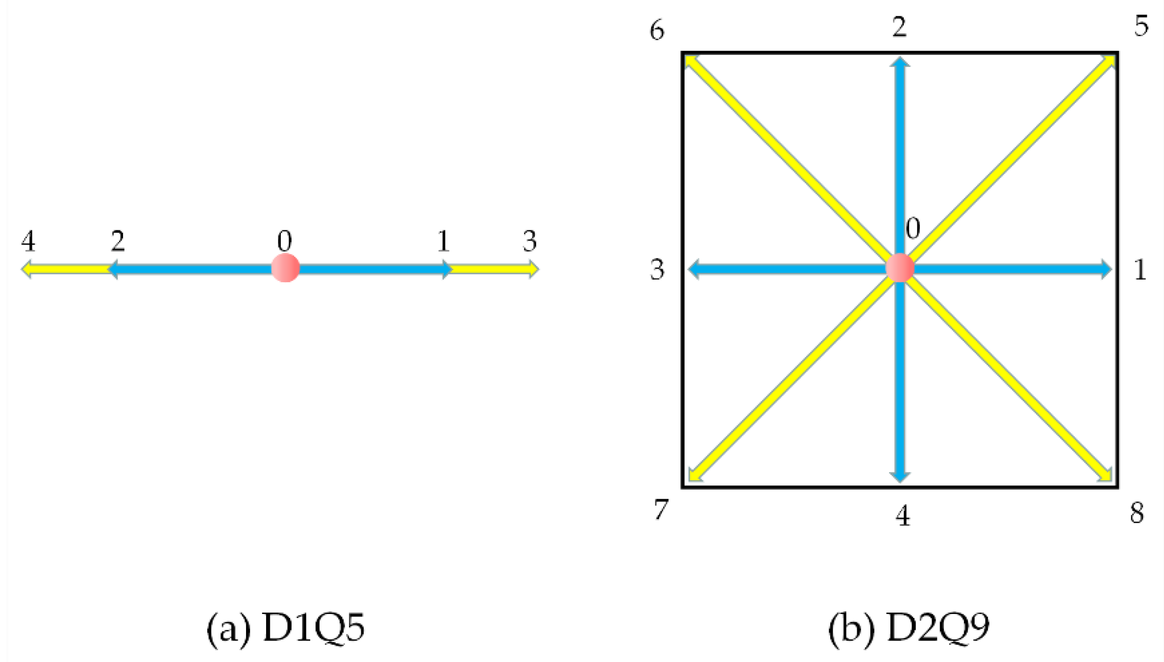
SRT-LBM is one of the most widely used LBE models based on the Bhatnagar-Gross-Krook (BGK) collision operator [38]. The particle velocity distribution function in the SRT-LBM model is discretized in multiple velocity directions. Constructing a single-relaxation-time (SRT) model hinges on the appropriate selection of equilibrium distribution functions. The specific form of equilibrium distribution functions is contingent upon the construction of the chosen discrete velocity model (DVM). The symmetry of the discrete velocities determines whether the corresponding lattice Boltzmann model can accurately recover the macroscopic equations to be solved. Hence, the selection of the DVM constitutes a pivotal aspect in the construction of the SRT-LBM. The DnQm model (where n represents the spatial dimension and m indicates the number of discrete velocities) proposed in reference [39] serves as the fundamental model for SRT-LBM. In the case of n=1, the commonly used DVM is the D1Q5 model (shown in Figure 1(a)), and for n=2, the prevalent choice for the DVM is the D2Q9 model (shown in Figure 1(b)).
The governing equations for SRT-LBM based on the DnQm can be expressed as follows:
f t + ξ × f = - 1 τ f - f e q f n e q = f - f e q ,
where f = f(ξ,x,t) represents the particle distribution function, t is time, x is spatial position, ξ is particle velocity, τ is the relaxation time, f neq stands for the non-equilibrium part of the particle distribution function, and f eq denotes the equilibrium distribution function. The specific formulas are as follows:
f e q = ρ ( 2 π R T ) D 2 e x p - ξ - u 2 2 R T ,
where R represents the gas constant, T stands for temperature, D denotes spatial dimension, and ρ signifies the density associated with fluid pressure p, and ρ is given by ρ=p/RT, while u represents fluid velocity.
Since the particle velocity ξ is continuous, the DnQm discrete velocity Boltzmann model is used in this paper for computational convenience. Consequently, Equation (2) is transformed into the following discrete form:
f a e q = ρ ω a 1 + e a × u c s 2 + ( e a × u ) 2 2 c s 4 - u 2 2 c s 2 ,
where cs= RT represents the lattice speed of sound, and ωa stands for the lattice weight coefficient.
In D1Q5 discrete velocity Boltzmann model, the discrete velocities ea is shown below:
e a = e [ 0 , 1 , - 1 , 2 , - 2 ] , ω a = 1 2 , e a = 0 1 6 , e a = 1 , - 1 1 12 , e a = 2 , - 2
where ea denotes the direction of velocity discretization, and ωa stands for the weight associated with the lattice direction, a=0, 1, 2, 3, 4.
In D2Q9 discrete velocity model, the discrete velocities ea satisfy the following:
e a = ( 0 , 0 ) a = 0 c ( c o s [ ( a - 1 ) π 2 ] , s i n [ ( a - 1 ) π 2 ] ) a = 1 , 2 , 3 , 4 2 c ( c o s [ ( a - 1 ) π 4 ] , s i n [ ( 2 a - 1 ) π 4 ] ) a = 5 , 6 , 7 , 8
where ea represents the direction of velocity discretization, c = δ x / δ t , where δx and δt are grid spacing and time step, respectively. The weight coefficient ωa follows the condition:
ω 0 = 4 9 , ω 1 = ω 2 = ω 3 = ω 4 = 1 9 , ω 5 = ω 6 = ω 7 = ω 8 = 1 36 .
In order to recover macroscopic physical quantities from the particle distribution functions in the mesoscale equation, the equilibrium distribution function faeq needs to satisfy the following moment equations:
a f a e q = ρ a f a e q e a = ρ u .
Where the macroscopic pressure is directly obtained from the equation of state as p=ρcs2 and cs is the lattice speed of sound, typically set to 1 / 3 .

2.2. Network Structure

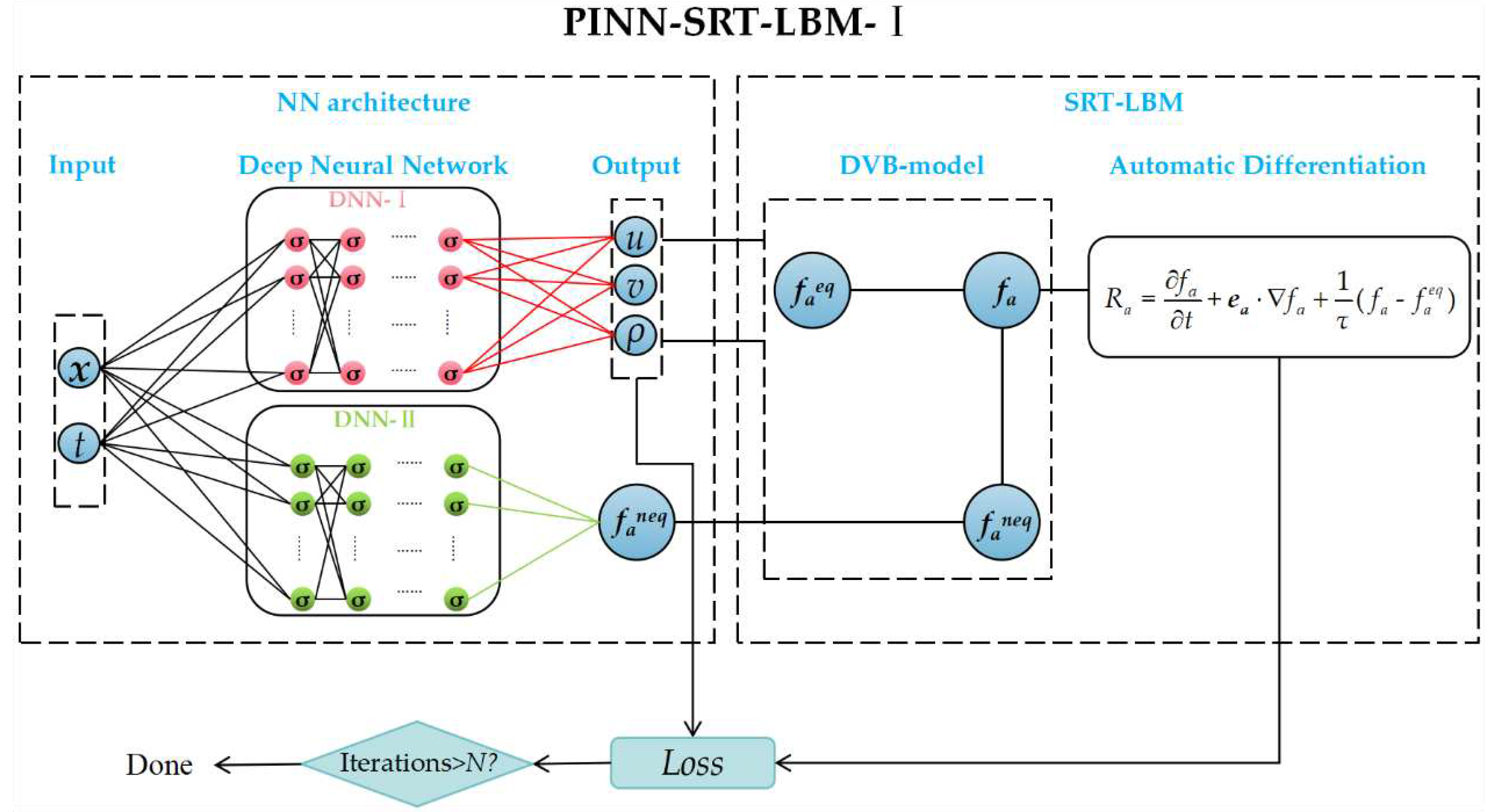
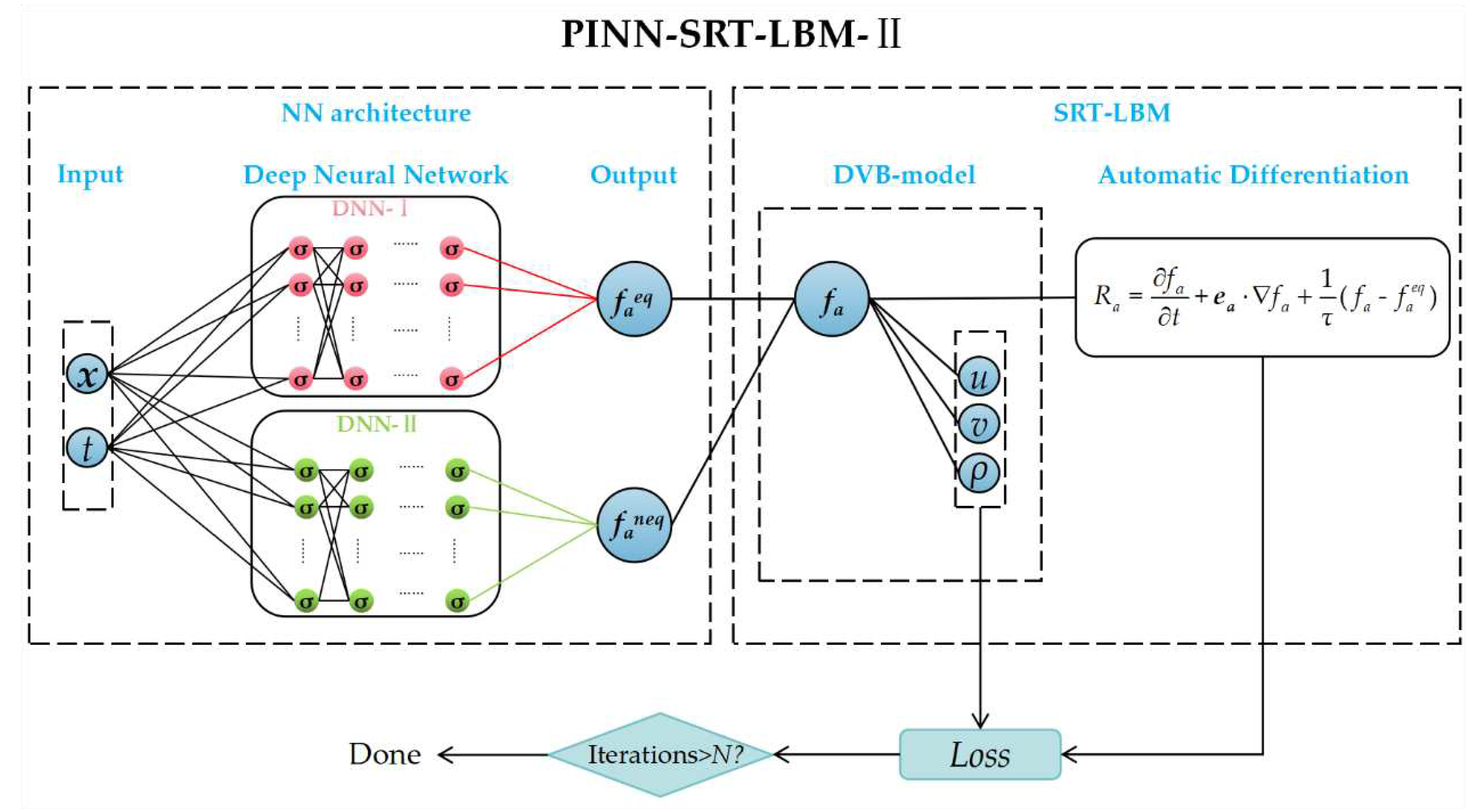
In this part, the neural network architecture of combining SRT-LBM with PINNs is presented. To supplement the practical application of PINNs in the context of combining mesoscopic physical models, this paper proposes two variants of the PINN-SRT-LBM model, namely, PINN-SRT-LBM-I and PINN-SRT-LBM-II, based on distinct physical driving mechanisms from a mesoscopic physics perspective (refer to Figure 2 and Figure 3).
As shown in Figure 2, the PINN-SRT-LBM-I model consists of a neural network architecture and the physical informed function SRT-LBM. The neural network structure of the PINN-SRT-LBM-I model comprises network inputs x and t, two deep neural networks labeled as DNN-I and DNN-II, along with the macroscopic quantities output by DNN-I and the non-equilibrium distribution function faneq output by DNN-2. The input x represents location information and t represents time information. The network components DNN-I and DNN-II consist of deep neural networks with adjustable parameters. DNN-I and DNN-II are the fundamental neural networks that make up PINN-SRT-LBM. The activation function of the neurons, denoted as σ, is configured as the hyperbolic tangent function (tanh) within the model. DNN-I is employed for the prediction of macroscopic quantities, while DNN-II is utilized for approximating the non-equilibrium distribution function. During training, the model's performance can be adjusted by configuring the network's depth and width. The output section encompasses the macroscopic quantities u, v, and ρ predicted by DNN-I, as well as the approximated non-equilibrium distribution function faneq from DNN-II.
The physical informed function of the PINN-SRT-LBM-I (the SRT-LBM component in Figure (2) is initially derived using the DVM to obtain the distribution function. Subsequently, employing the automatic differentiation capability (Autograd) provided by PyTorch, the PDEs specified in the SRT-LBM formulation are computed to yield residual values. These residuals, in combination with the macroscopic quantities, formulate the Mean-Square Loss. The iterative process continues until reaching the maximum iteration count N. The definition of the residuals is obtained from Equation (1).
The construction of the PINN-SRT-LBM-II model is depicted in Figure 3. The neural network structure of this model is the same as the PINN-SRT-LBM-I model. However, in the neural network output section, DNN-I approximates the equilibrium distribution function faeq, while DNN-II approximates the non-equilibrium distribution function faneq. The physical informed function of the PINN-SRT-LBM-II model employs the DVM. It transforms the equilibrium distribution function faeq and the non-equilibrium distribution function faneq, as defined in Equation (6), into macroscopic quantities u, v, and ρ. These quantities are used to compute residuals through automatic differentiation. This implementation process is contrary to that of the PINN-SRT-LBM-I model. The primary distinction between the PINN-SRT-LBM-I and PINN-SRT-LBM-II models lies in the neural network outputs and the physical informed function. Simply put, the difference between the PINN-SRT-LBM-I model and the PINN-SRT-LBM-II model is evident in their different network outputs. The former yields macroscopic quantities, while the latter provides microscopic quantities.
This difference in the PINN-SRT-LBM model stems from the variation in input values when applying physical constraints using the DVB model. Notably, the structure of the deep neural networks (DNN-I and DNN-II) outputs should be adjusted based on the chosen DVM. For instance, if a D2Q9 DVM is chosen, then the equilibrium distribution function and non-equilibrium distribution function (f eq and f neq) should correspond to the nine discrete velocity directions.
In both PINN-SRT-LBM-I and PINN-SRT-LBM-II, these distribution functions follow the relationship fa (x,t) = faeq + faneq.
During the process of network training, challenges such as vanishing gradients (where gradients become extremely close to 0) and exploding gradients (where gradients become excessively large) can arise. These issues can lead to ineffective or counterproductive gradients during backpropagation. Consequently, in this work, the initialization method chosen for network parameters is Xavier initialization [40]. This technique is employed to mitigate the impact of gradient-related problems and contribute to the stability of the training process.
The Xavier initialization demonstrates exceptional performance when the activation function is set to tanh. Xavier initialization significantly impacts the convergence speed and final performance of neural networks, potentially aiding in learning deeper levels of abstract features. Additionally, the range of weights is effectively constrained by Xavier initialization, thereby preserving the consistency of input-output data distribution variances. This special initialization helps prevent overfitting and ensures a high degree of model stability.
The formulas for Xavier initialization in both uniform and Gaussian distributions are as follows:
W ~ U [ - 6 n i + n i + 1 , 6 n i + n i + 1 ]
W ~ U [ 0 , 2 n i + n i + 1 ] ,
where W represents the initialized weights of the neural network and ni signifies the size of the ith layer in the network. These initialization formulas contribute to maintaining a balanced distribution of weights, promoting better training and generalization capabilities of the neural network.

2.3. Loss Function and Optimization Method

Simulation of the inverse problem in fluid dynamics using the PINN-SRT-LBM-I and PINN-SRT-LBM-II models proposed in this paper, the physical constraints of SRT-LBM should be integrated into the training by minimizing the following loss function:
L = β 1 L S R T + β 2 L M L S R T = 1 N t r a i n a = 0 Q - 1 j = 1 N t r a i n R a ( x j , t j ) - 0 2 , L M = 1 N t r a i n n = 1 N t r a i n Φ ( x n , t ) - Φ * ( x n , t ) 2 ,
where Ra(x,t) represents the residual values corresponding to the Boltzmann-BGK equation, which can be computed according to Equation (1). Constructing the residual calculation formula as follows:
R a = f a t + e a f a + 1 τ ( f a - f a e q ) , a = 0 , 1 , 2 , ... , 8
In the loss function (Equation (10)), this work introduces a set of weighting coefficients (β1, β2) to address the issue of disparate error magnitudes among different terms. These weighting coefficients ensure that distinct components of the loss function hold equal importance during the optimization process.
Moreover, within the loss function, L, LSRT and LM respectively correspond to the loss associated with the entire loss function, the loss stemming from the residuals of the SRT-LBM, and the loss concerning the macroscopic quantities of the training points. Ntrain pertains to the number of training points within the computational domain. Φ signifies the macroscopic quantities u, v, ρ. Importantly, the loss function in the introduced PINN-SRT-LBM-I and PINN-SRT-LBM-II models adheres to an identical configuration.
During the training of the neural network models, two distinct neural network optimizers are employed: Adam [44] and L-BFGS-B. These two optimizers play a crucial role in the model training process, aiding in minimizing the loss function and updating the model's parameters.
In the training phase, a transfer learning approach using the Adam and L-BFGS-B optimizer combination was adopted to accelerate model training. Initially, during the early stages of training, the Adam optimizer is utilized with a dynamically adjusted learning rate. After the loss value is less than the pre-defined value, the optimization transitions to the L-BFGS-B optimizer and iterates to the set maximum number of iterations. This hybrid optimization strategy aims to optimize the neural network model more efficiently by leveraging the strengths of both optimizers.

2.4. Dataset Construction

In order to evaluate the model performance, the proposed PINN-SRT-LBM-I and PINN-SRT-LBM-II models were tested through simulation experiments involving 1D and 2D inverse problems in fluid mechanics. For the 1D case, the Sod shock tube problem was selected, while for the 2D cases, lid-driven cavity flow and flow around circular cylinder were selected. This section will introduce the construction of the datasets.
Initially, for the 1D Sod shock tube case, precise solution data was obtained from Riemann solvers [41]. In the case of the 2D lid-driven cavity flow, we adapted the numerical solution from the example code provided in reference [42] to create an appropriate dataset format. As for the 2D flow around circular cylinder dataset, an open-source dataset from reference [25] was utilized.
In the data processing phase, data manipulation libraries and tools were utilized for tasks such as data cleansing, preprocessing, and feature extraction. The data underwent normalization and smoothing processes to better suit subsequent data analysis and modeling tasks.
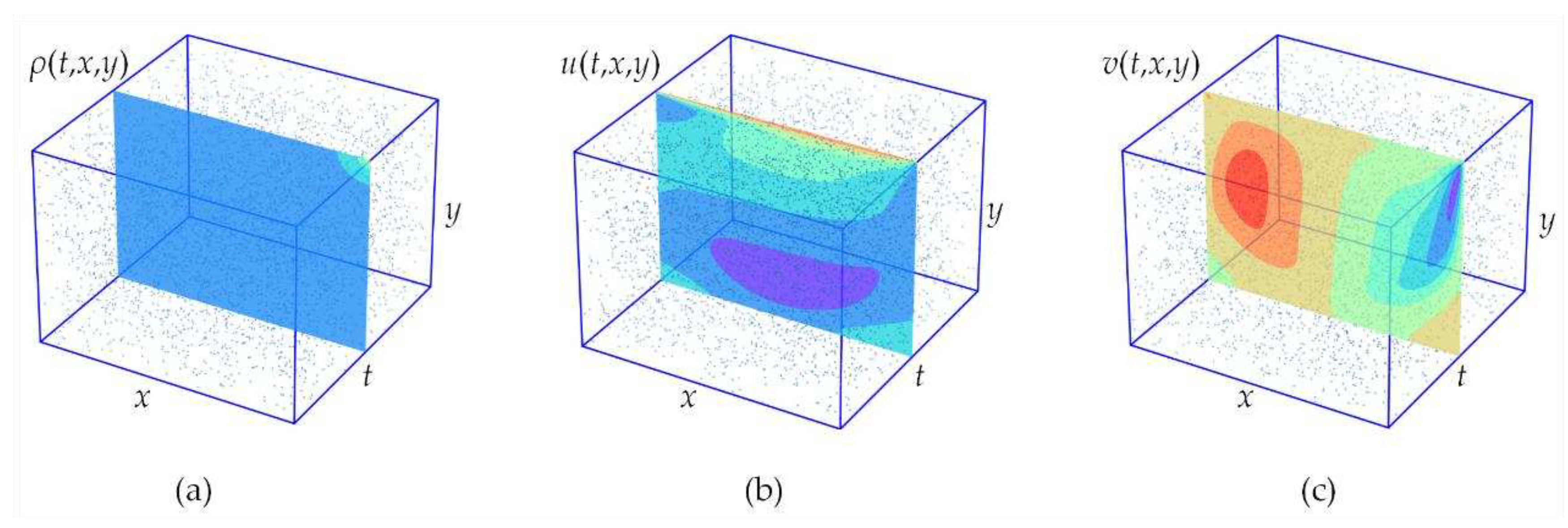
Ultimately, the processed data was saved in the standardized format of Matlab data storage. The dataset encompasses crucial physical variables along with accompanying annotation information to facilitate research and analysis across different problem domains. As a reference, a schematic illustration of the dataset structure, exemplified by lid-driven cavity flow, is presented in Figure 4. This includes representative time slices of density distribution ρ(t,x,y) , as well as velocity components u(t,x,y) and v(t,x,y).
The detailed information about the datasets used in the experiments is presented in Table 1, where Xexact represents the coordinate values of the points selected within the computational domain. The ρexact represents the recorded density of training points at different time steps, Uexact corresponds to the velocity of points at each time step. Di , where i = 1,2, denotes the dimensionality, either 1D or 2D. Ns, NL and Ncy ​respectively indicate the number of training points in the Sod shock tube, lid-driven cavity flow, and flow around circular cylinder datasets. Ts , TL, Tcy correspond to the number of time steps in the Sod shock tube, lid-driven cavity flow, and flow around circular cylinder datasets. To emphasize the model's ability to learn from scattered and sparse training data, this paper opted for Ns = 1000, NL = 4225, Ncy = 5000. The number of time slices was set as follows: Ts = 100, TL = 100 and Tcy = 200. Notably, when employing our proposed model to simulate fluid mechanics inverse problems, only 1% of the available data points are utilized as training points.

3. Results

This section presents a comprehensive experimental validation and analysis of the PINN-SRT-LBM-I and PINN-SRT-LBM-II using classical CFD cases. In order to ensure accuracy, the experiments encompass both 1D and 2D cases, specifically addressing the sod shock tube case in the 1D scenario, and the lid-driven cavity flow and flow around circular cylinder cases within the 2D scenario.
The computational resources employed in this paper include NVIDIA Titan X based on the Pascal architecture. The card offers a floating-point computational capacity of 11 TFLOPS, a memory capacity of 12288MB, 3584 CUDA cores, and a clock frequency of 1.53 GHz.

3.1. Sod Shock Tube

The shock tube is a type of experimental apparatus that serves as a significant means for studying nonlinear mechanics. The sod shock tube problem is a commonly employed test case in CFD, smoothed particle hydrodynamics (SPH), and similar methods. It serves to assess the efficacy of specific computational approaches and exposes potential shortcomings within methods, such as numerical schemes. The shock tube for the sod shock tube problem is divided into two regions, left and right, separated by a thin membrane. When the membrane ruptures (T=0), a shock wave propagates from the left to the right, while an expansion wave moves from the right to the left [43].
In this part, this paper employed three methods: PINN-SRT-LBM-I, PINN-SRT-LBM-II, and DNNs, to simulate the density field, pressure field, and velocity field within the computational region of the Sod shock tube at T=100.
For the sod shock tube problem, the D1Q5 DVM was utilized. The model configuration is shown in Figure 1(a), and the model parameters are established according to Equation (4).
The initial values for the exact solution are set as follows:
( ρ L , u L , p L ) = ( 0.125 , 0.0 , 0.1 ) 0 < x < 0.5 ( ρ R , u R , p R ) = ( 1.0 , 0 , 1.0 ) 0.5 < x < 1.0 .
In the experiments, the density and length are respectively set as:ρ0 = 1 and L0 = 1. The grid size is set as Δx = 1/1000, the time step length is Δt = 0.001, the total duration is t = 0.1, and the number of time slices is T = 100. The position of the shock is chosen at x = 0.5.
To simulate the density ρ, pressure p, and velocity u, we divide the entire simulation duration of t = 0.1 into T time slices and extract 1000 training points. This constitutes 1% of the total available data. These points are employed as internal observations for solving the inverse problem and are used for training, while the remaining data is reserved for validation.
For the DNN-I and DNN-II in both the PINN-SRT-LBM-I and PINN-SRT-LBM-II models, the neural network configuration consists of 8 hidden layers with 20 neurons each, utilizing the tanh activation function. The DNNs employed for comparison are similarly structured with 8 hidden layers and 20 neurons per layer, utilizing the tanh activation function. The weight coefficients in the loss function are set as (β1, β2) = (1, 1). The max iteration is set to 80000, and the optimizer follows the Adam + L-BFGS-B combination.
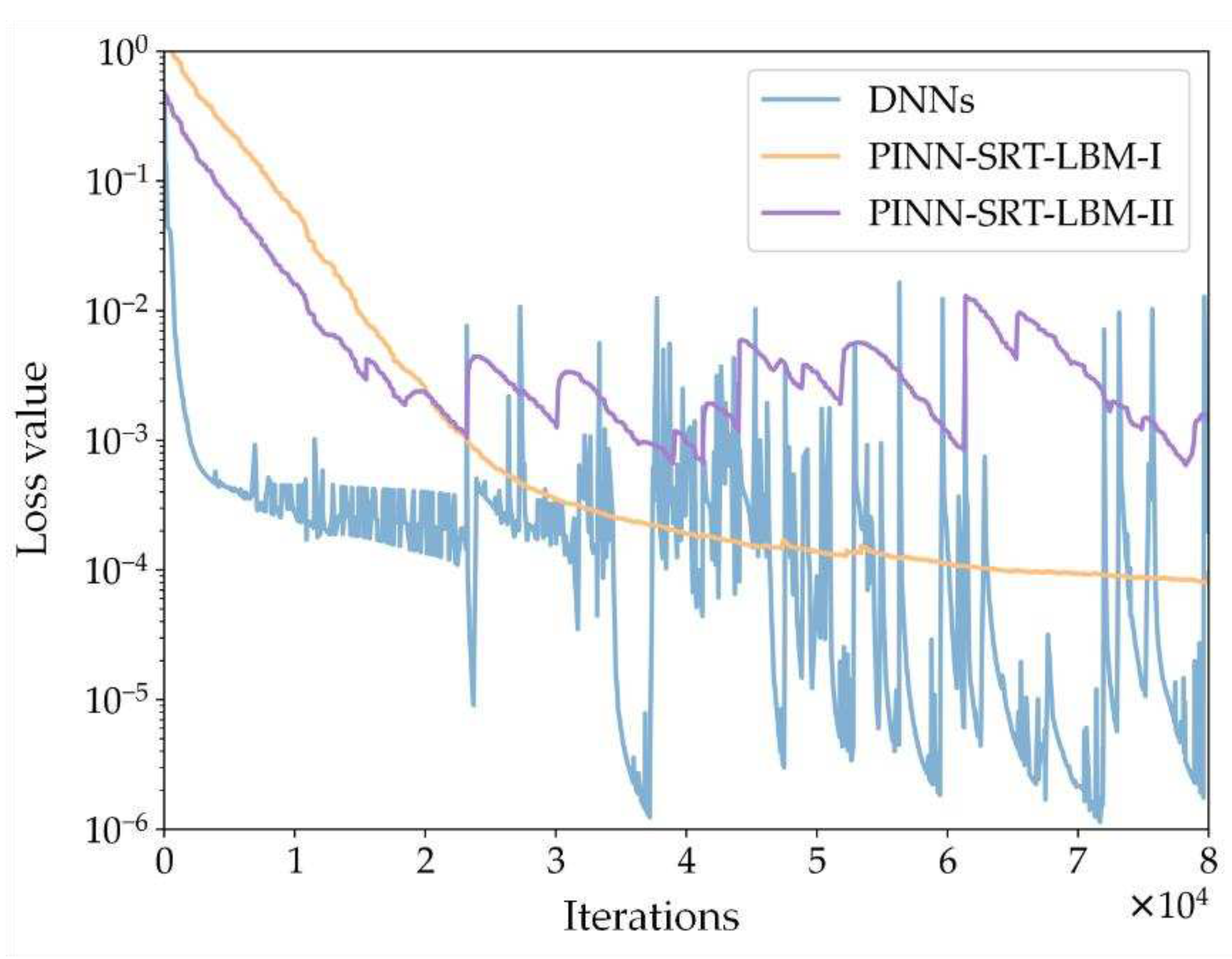
Figure 5 shows the comparison of training loss curves for the Sod shock tube inverse problem simulation using three methods: PINN-SRT-LBM-I, PINN-SRT-LBM-II, and DNNs. The depicted oscillation amplitude and convergence range of the training loss curves in the graph indicate a significant advantage of the PINN-SRT-LBM-I.
To further validate the superiority of the PINN-SRT-LBM-I model, Table 2 presents the relative errors L2 of the simulation results obtained using the three methods with respect to the reference solution. Here, erru, errp, and errρ represent the relative errors L2 for velocity, pressure, and density, respectively.
The data in Table 2 reveals that the PINN-SRT-LBM-I model exhibits higher accuracy in solving the sod shock tube problem compared to DNNs and PINN-SRT-LBM-II. This advantage translates to more precise simulation results within the predicted region and enhanced stability.
The definition of the relative error L2 is given by:
e r r L 2 = 1 N i = 1 N | y i - y i * | 2 ,
where yi represents the predicted value, yi* represents the exact value, and N is the number of prediction points.
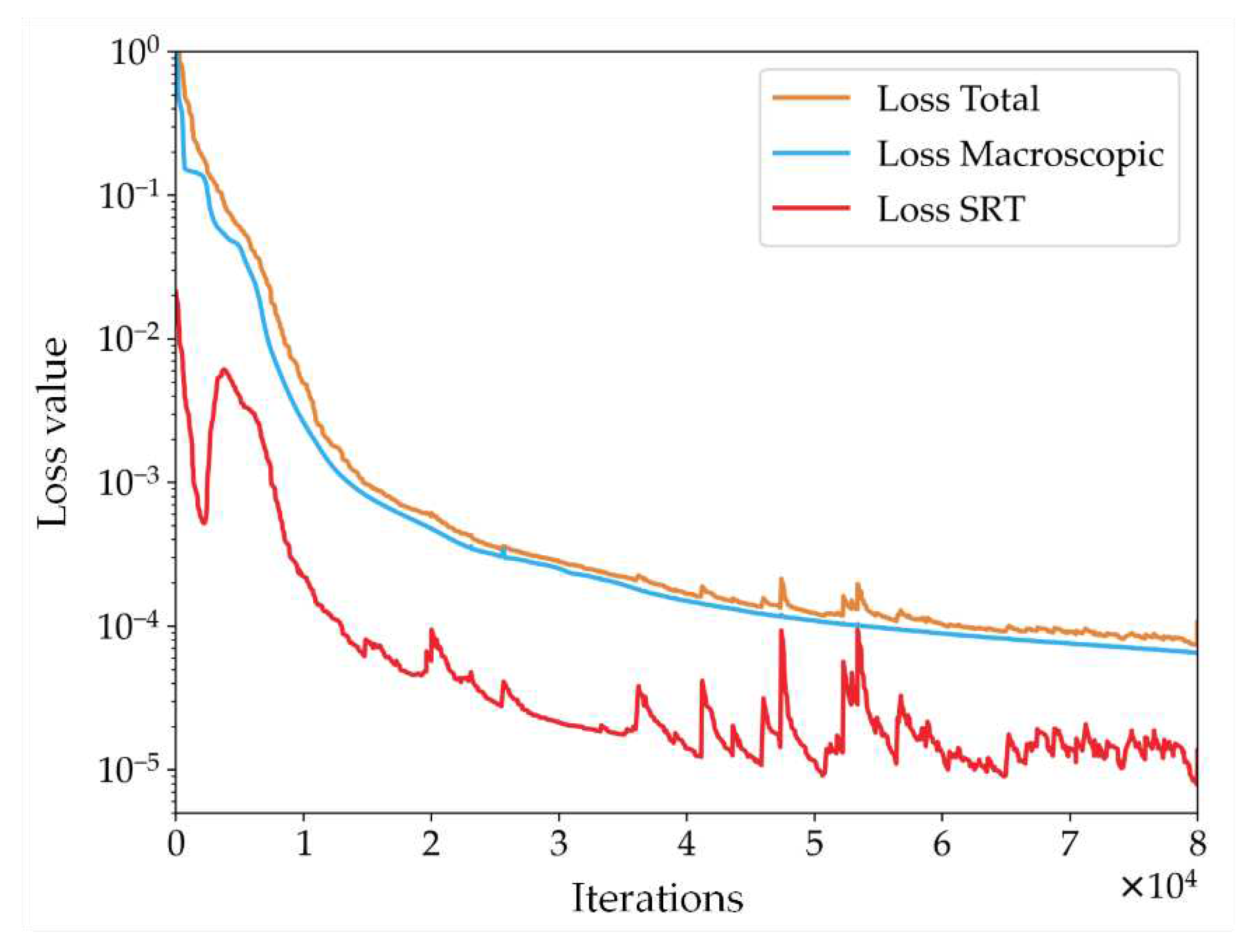
Furthermore, Figure 6 presents a schematic curve depicting the variation of the loss function values during training for the PINN-SRT-LBM-I model. The curves include Loss SRT, representing the loss function of the residual values from the SRT-LBM's PDEs; Loss Macroscopic, depicting the loss function of the macroscopic quantities at training points; and Loss Total, the summation of the preceding two. By comparing the training loss curves over iterations, one can observe the substantial influence of the Loss SRT curve on the Loss Total curve. This validates that the proposed model in this paper enforces the physical constraints on neural network training.
In Figure 7, a comparison is presented between the predicted pressure p, density ρ, and velocity u by the PINN-SRT-LBM-I model and the exact solutions.
The results in Figure 7 indicate that the predicted physical quantities closely match the exact solutions, highlighting the effectiveness of the PINN-SRT-LBM-I in simulating the Sod shock tube problem. However, it's worth noting that when abrupt changes occur in the physical quantities over a short time, the predictions display oscillations. This suggests that the neural network's ability to learn such rapid variations is limited due to the nonlinear nature of these changes. To improve this aspect, exploring networks with stronger nonlinear learning capabilities is advisable.

3.2. Lid-Driven Cavity Flow

In this section, we conduct experimental validation concerning a classic problem in 2D scenarios: the incompressible steady-state lid-driven cavity flow. The experiments are conducted in a 2D cavity domain, denoted as Ω = (0,1) × (0,1). The number of time slices is set to T=100,A continuous and constant rightward initial velocity of U=0.1 is applied at the upper boundary of the cavity. Non-equilibrium extrapolation is employed for the boundary conditions. The initial density of the flow field is ρ0=1, and the governing equation is represented by Equation (1). The DVM utilizes the D2Q9, as illustrated in Figure 1(b).
There are four datasets of training data, each comprising 4225 randomly selected spatiotemporal training points within the computational domain, are gathered at Re = 400, 1000, 2000, 5000. The reference solutions for the velocity field and density field of these points are derived from reference [44]. The horizontal velocity and vertical velocity are denoted as u(T,x,y) and v(T,x,y) respectively, while the density field is represented as ρ(T,x,y). The weights for the loss function are set as (β1, β2) = (1,1). In this reference solution, 1% of the entire dataset will be used for training, with the remaining portion utilized for validating the predictive outcomes. Considering that the flow field of the lid-driven cavity under the specified Reynolds numbers attains a steady state we focus solely on simulating the flow field at the final time step (T=100).
To train the models for the experimental cases, the foundational components DNN-Ⅰ and DNN-Ⅱ of both the PINN-SRT-LBM-I and PINN-SRT-LBM-II models are configured with 8 hidden layers, each containing 40 neurons and employing the hyperbolic tangent (tanh) activation function. The parameters of the contrasting DNNs network are set to 8 layers with 40 neurons per layer. The maximum number of training iterations is established at 80000, and the training process employs the Adam + L-BFGS optimizer. Notably, for the DNNs in this experiment, the SGD optimizer will be utilized in the pursuit of potentially enhanced performance.
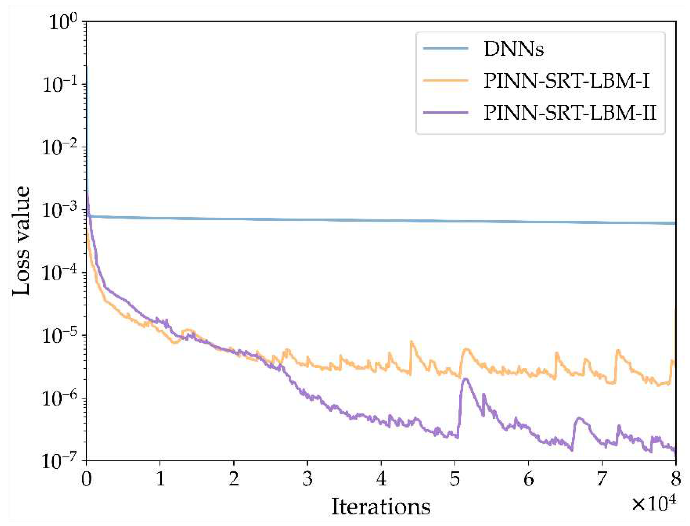
The results shown in Figure 8 unveil the characteristics of the training loss curves for the three methods: PINN-SRT-LBM-I, PINN-SRT-LBM-II, and DNNs, when simulating the lid-driven cavity flow. Notably, the loss value of DNNs experiences a rapid descent to below 1×10⁻³ followed by an onset of overfitting. Meanwhile, the loss value of the PINN-SRT-LBM-II model converges within a range one order of magnitude smaller than that of the PINN-SRT-LBM-I model. This deduction is grounded in the fact that the PINN-SRT-LBM-II model directly leverages deep neural networks to approximate both equilibrium and non-equilibrium distribution functions. When tackling the 2D inverse problem of the lid-driven cavity flow, the PINN-SRT-LBM-II model is anticipated to excel in capturing intricate details of the underlying physical distribution patterns compared to both DNNs and the PINN-SRT-LBM-I model. In order to empirically validate our conjecture, Table 3 presents the relative errors L2 for the results obtained by the PINN-SRT-LBM-I, PINN-SRT-LBM-II, and DNNs when simulating at Re =1000 and T =100.
In Table 3, erru, errv, and errρ respectively denote the relative errors L2 of u, v, and ρ. The results notably illustrate that the relative errors L2 of the predictions generated by the PINN-SRT-LBM-II model are approximately one order of magnitude lower than those of both DNNs and the PINN-SRT-LBM-I model.
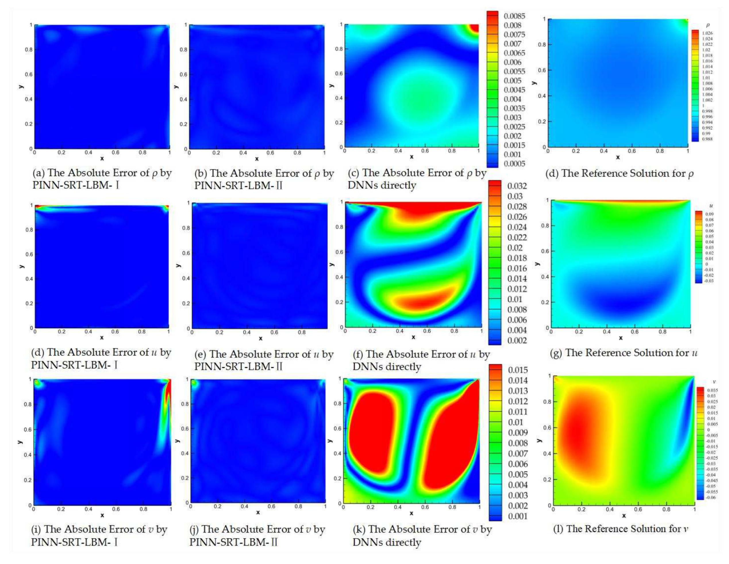
For a more comprehensive comparison of the accuracy of different models, Figure 9 displays the visualizations of absolute errors between the reference solution and the simulated results by PINN-SRT-LBM-I, PINN-SRT-LBM-II, and DNNs. The first column (a), (e), (i) presents the visualizations of absolute errors for PINN-SRT-LBM-I; the second column (b), (f), (j) displays the visualizations of absolute errors for PINN-SRT-LBM-II; and the third column (c), (g), (k) showcases the visualizations of absolute errors for DNNs. The absolute error images reveal the observable discrepancies between predicted and reference values. Finally, the last column (d), (h), (l) provides the visual representations of the reference solutions.
As for the absolute error, let Ypred(t,x,y) denote the predicted value at coordinates (x,y) for T=t, and Yexact(t,x,y) represent the reference solution value at the same coordinates and time. The absolute error function is defined as follows:
E a b s ( t , x , y ) = | Y p r e d ( t , x , y ) - Y e x a c t ( t , x , y ) | ,
where Eabs(t,x,y) represents the absolute error function, Ypred(t,x,y) denotes the predicted value at time T=t and position (x,y), and Yexact(t,x,y) signifies the reference solution value at time T=t and position (x,y). Subtracting these two values and taking the absolute value yields the absolute error at point (x,y) during the time slice T=t.
From the results shown in Figure 9 and the relative error L2 presented in Table 3, a reasonable inference can be made that DNNs lack the capability to address the inverse problem of 2D lid-driven cavity flow. Moreover, it can be observed that the PINN-SRT-LBM-I model, when employed to simulate the 2D lid-driven cavity flow, struggles to capture the characteristics of physical quantities at the boundaries. This phenomenon arises due to the significant variations of physical quantities in proximity to the boundaries. Consequently, the model encounters greater difficulty in learning the evolution patterns near these boundaries compared to other regions, leading to elevated levels of error.
It is worth noting that in the simulations of CFD, the Reynolds number exerts a substantial influence on the results. Thus, in the experimental cases of this section, we have included investigations of the inverse problem of lid-driven cavity flow under various Reynolds numbers.
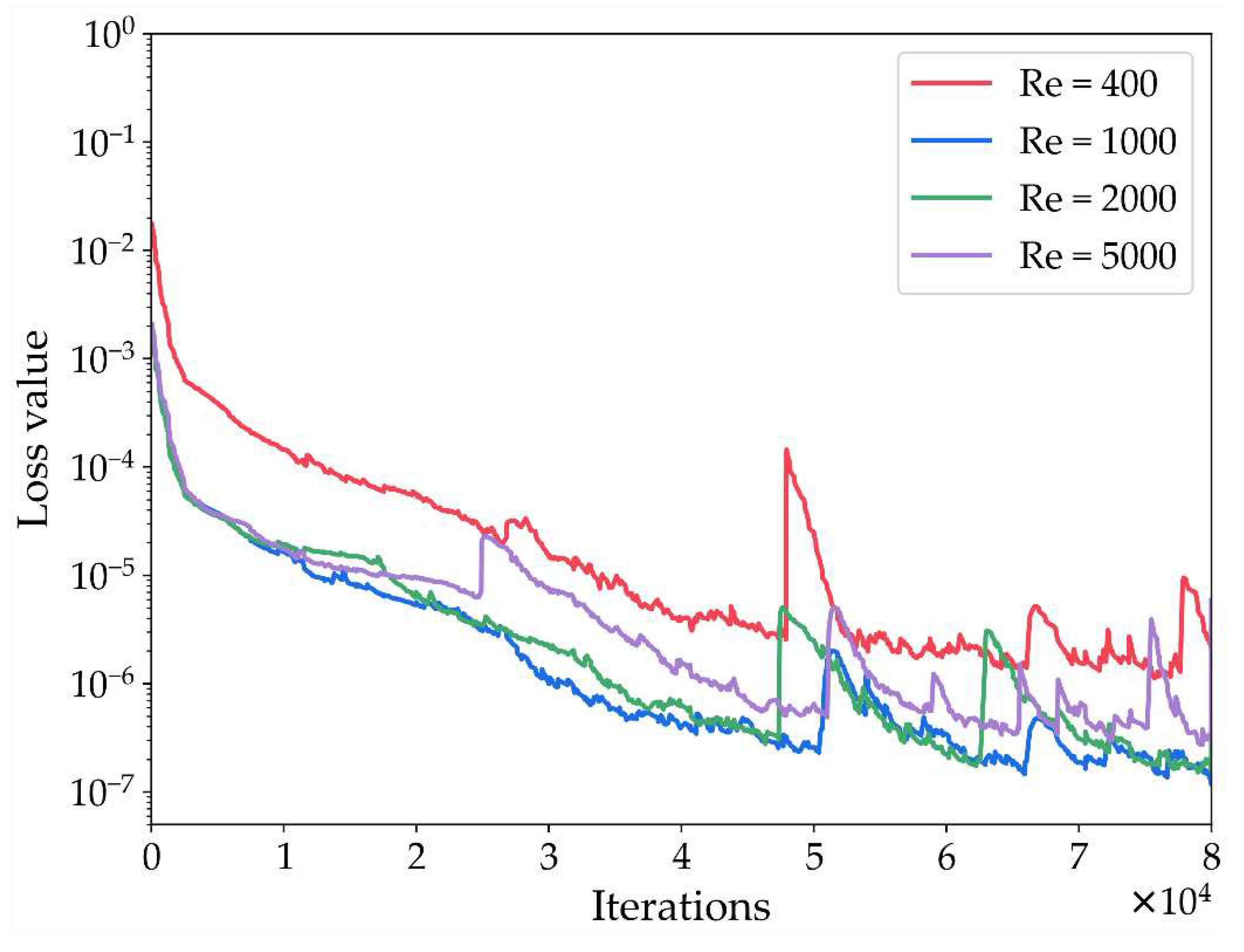
In the course of the experiments, four distinct Reynolds number values were considered: Re = 400, Re = 1000, Re = 2000, and Re = 5000. Predictions were made for the results at T = 100, which corresponds to the attainment of a steady state within the cavity. Using PINN-SRT-LBM-II to address predictions for different Reynolds numbers, the variation of the training loss curves with respect to time is depicted in Figure 10. Observing the trend of the loss value across iterations in Figure 10, it can be concluded that the convergence range of the model's loss value remains relatively consistent as the Reynolds number increases. This indicates that the PINN-SRT-LBM-II model exhibits stability across different Reynolds numbers and underscores its capacity for generalization.
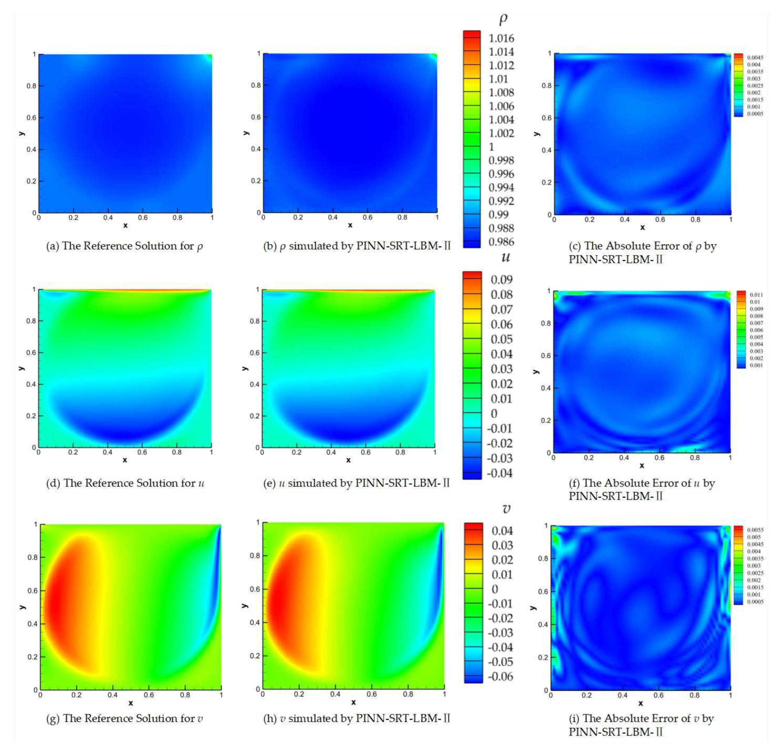
In Figure 11, we present the visual results of the predictions made by the PINN-SRT-LBM-II model and the reference solution for Re=5000 and T=100.
Figure 11(a), (b), and (c) respectively depict the visualizations of the reference solution ρ, the predicted ρ from the PINN-SRT-LBM-II model, and the visualization of the absolute error in the predicted ρ. Figure 11(d), (e), and (f) correspondingly represent the visualizations of the u for reference solution, the predicted u from the model, and the visualization of the absolute error in the predicted u using the PINN-SRT-LBM-II model. Similarly, Figure 11(g), (h), and (i) show the same pattern for v.
In Figure 11(b), (e), and (h), observe elevated absolute error values in regions near the cavity boundaries and the primary vortex. Notably, absolute errors surpass 10-2 at the cavity vertices, with errors near the primary vortex exceeding other areas by around 10-3. These discrepancies are attributed to the accumulation of errors and rapid changes in the physical distribution patterns.
Significantly, the absolute error results in the predicted density ρ are notably better than those for u and v in the results. Consequently, we can infer that regions with intense variations in physical patterns within the computational domain pose a challenge for the model's learning process. Moreover, the mesoscopic physics-based approach SRT-LBM imparts a distinct advantage to the model in accurately capturing the distribution patterns of ρ.
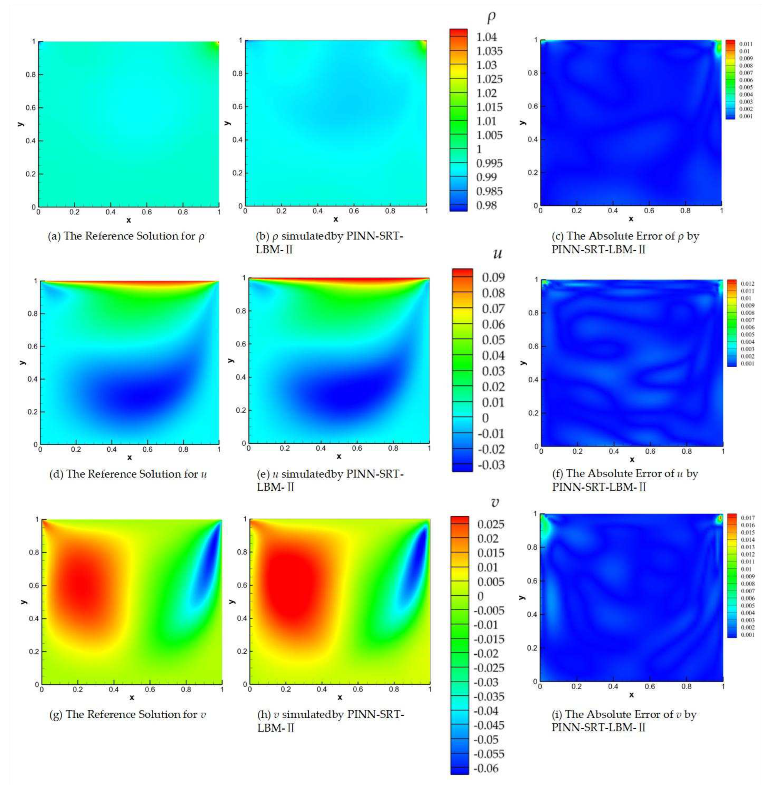
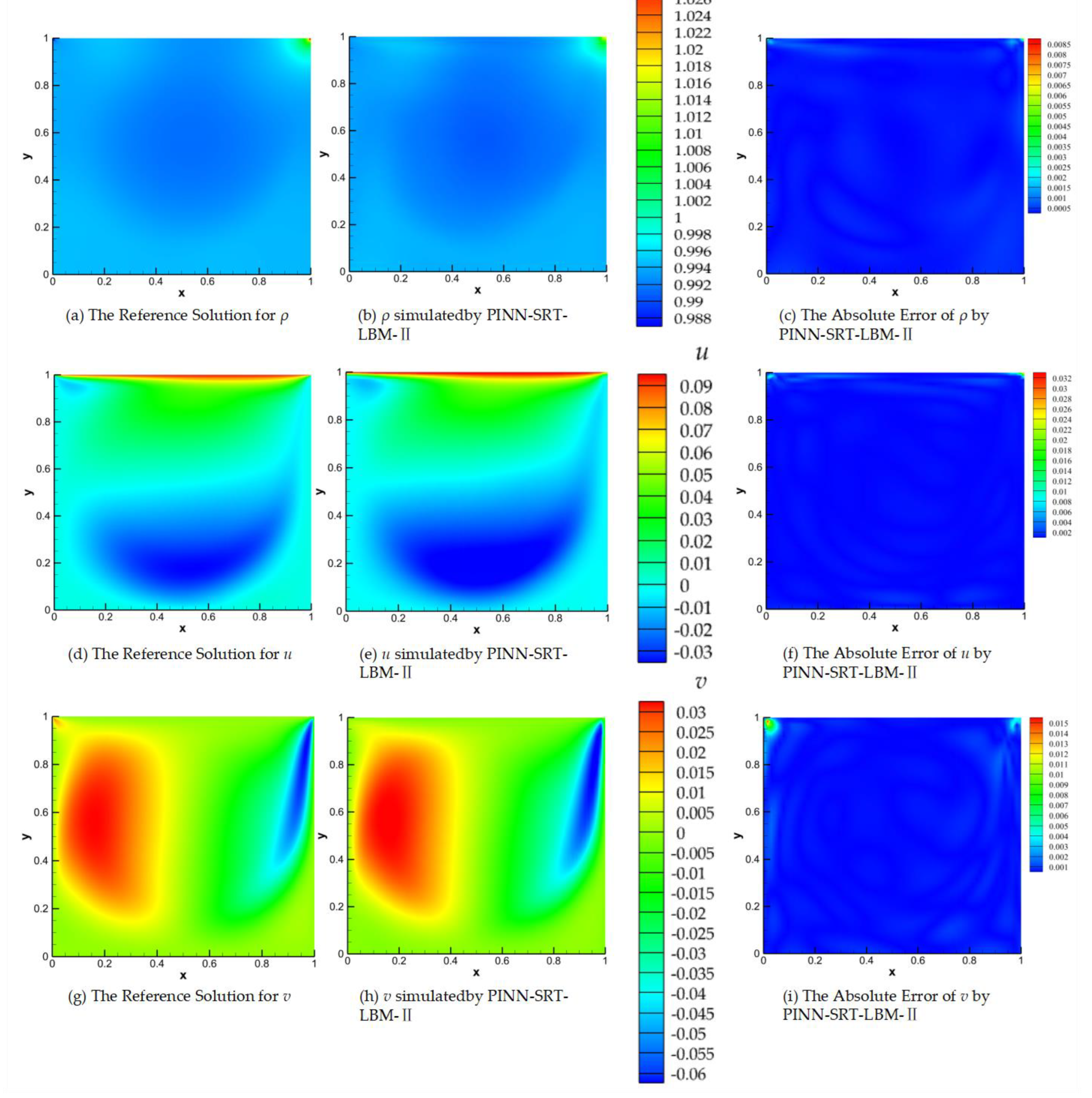
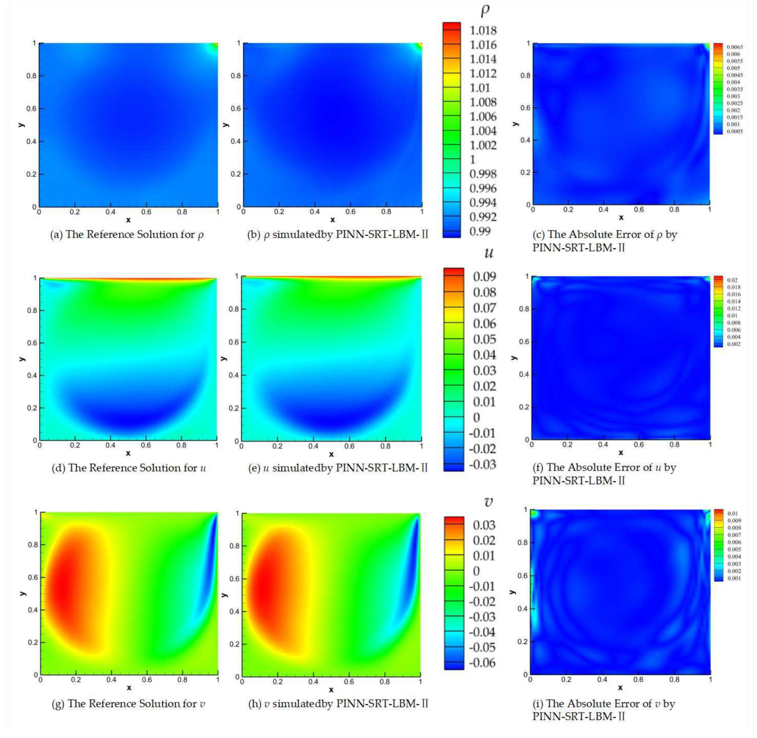
Consistent with the results presented in Figure 11, Figure 12, 13, and 14 depict visualizations of the reference solutions, model predictions, and absolute error results for Reynolds numbers Re=400, 1000, 2000 at T=100.
Through the progressive comparison of Figure 11, Figure 12, Figure 13and Figure 14 as the Reynolds number increases, a conclusion can be drawn. Given that the maximum absolute error remains below 10-2, the PINN-SRT-LBM-II model exhibits stability in simulating 2D lid-driven cavity flow. Furthermore, the comparative analysis of the results reveals that regions with more pronounced variations in physical distribution patterns tend to exhibit relatively higher absolute errors compared to other areas within the computational domain. This is due to the escalating nonlinearity with higher Reynolds numbers. However, the nonlinearity within the PINN-SRT-LBM-II model doesn't align perfectly. For instance, in Figure 11 (c), (f), and (i), there are irregular oscillations and uneven distribution of absolute errors within the simulation domain. As a result, prediction accuracy gradually decreases with higher Reynolds numbers. In order to address the above, attention should be given to countering overfitting during the model's training process [44].
To better assess the alignment between the results of the PINN-SRT-LBM-II model and the reference solution, this paper provides further comparison in Table 4 regarding the coordinate of main vortex center point. A represents the predictions from PINN-SRT-LBM-II, while B, C, and D correspond to the results presented in references [45,46,47].
The conclusion drawn from the coordinate of main vortex center point is that there exists a strong physical consistency between the prediction results and the reference solution. This signifies that the predictive results of the PINN-SRT-LBM-II model possess certain physical attributes, indicating the capability of the model to incorporate physical constraints, a manifestation of the synergy between the PINN-SRT-LBM-II model and SRT-LBM principles.
The relative errors L2 of the simulation results are shown in Table 5. The results indicate that with an increase in Reynolds number, the relative errors L2 do not exhibit a pronounced rise. This further substantiates the physical reliability and stability of PINN-SRT-LBM.
This work has differentiated the dimensions in which the PINN-SRT-LBM-I and PINN-SRT-LBM-II models are suited through comparative experiments. PINN-SRT-LBM has successfully conducted simulations of the inverse problem of 2D lid-driven cavity flow by learning from a sparse, randomly distributed 1% of data within the computational domain. This extension from one dimension to two dimensions demonstrates the applicability of dispersed temporal and spatial data, akin to passive scalar or limited data encountered in inverse problems, within the training of neural network models.

3.3. Flow around Circular Cylinder

In this part, this study have opted to employ a 2D flow around circular cylinder dataset provided by M. Raissi et al. in reference [25]. Flow around circular cylinder is a classic simulation problem in CFD. The purpose of conducting experiments in this subsection is twofold: to verify the performance of PINN-SRT-LBM in simulating the inverse problem of incompressible unsteady flows and to conduct comparative experiments with the work of other researchers. Open-source code exists for PINNs solving the inverse problem of fluid mechanics using the Navier-Stokes equations (referred to as PINN-NS in the subsequent). The performance of PINN-SRT-LBM in addressing the inverse problem of unsteady flows will be elaborated upon in detail within this part.
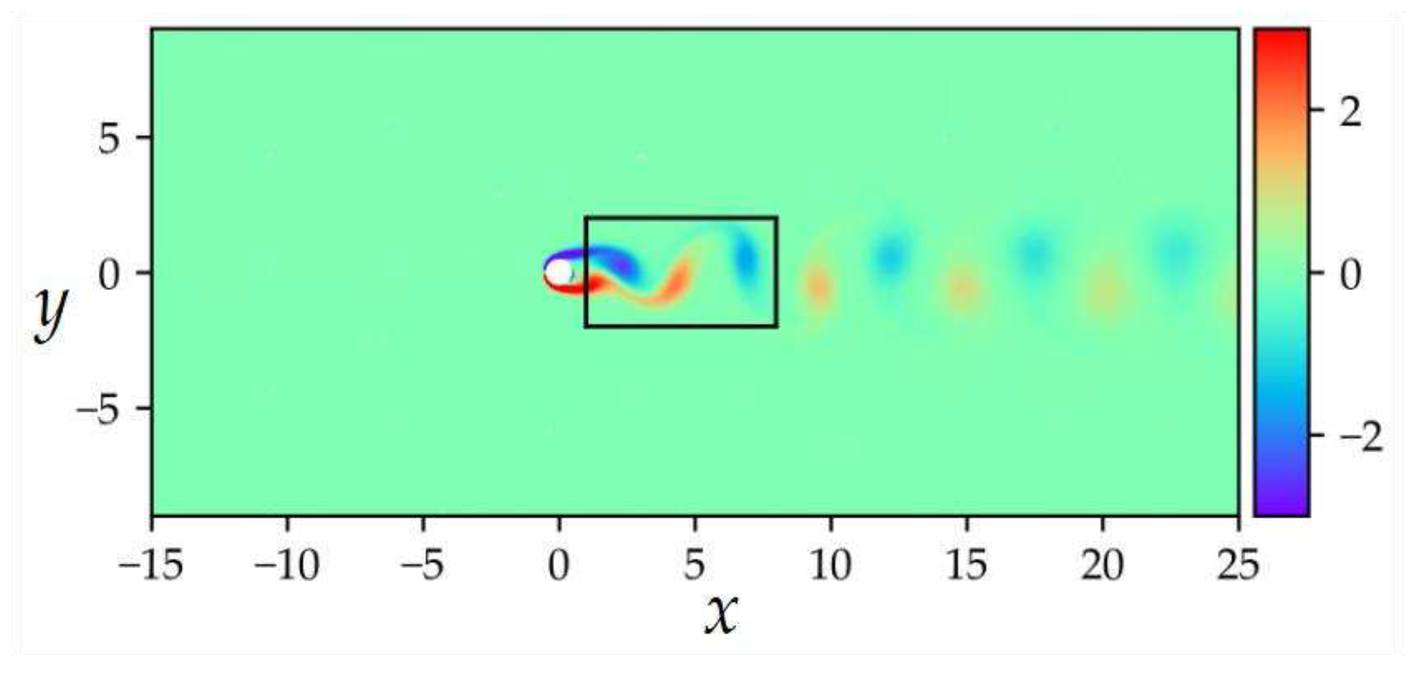
The dataset was set up with Re = 100, focusing on the wake region of the flow around circular cylinder. The dataset contained 5000 sampled training points, with a total of T = 200 time slices. For simplicity, the data collection was confined to a rectangular region downstream of the cylinder, as shown in Figure 15. The solver employed in this case was the spectral/hp element solver NekTar [48]. Since the dataset only contained velocity and pressure, the focus in this part's experiment was solely on simulating the velocity u(t,x,y) and v(t,x,y) within the sampled region.
This case assumes a uniform freestream velocity profile is imposed at the left boundary of the domain Ω = (-15,25) × (-8,8). A zero-pressure outflow condition is applied at the right boundary, 25 units downstream of the cylinder. The top and bottom boundaries of the domain adopt periodic boundary conditions. The initial velocity of the fluid is U=1, cylinder diameter D=1, and viscosity coefficient ν = 0.01. The system displays periodic steady state features characterized by asymmetric vortex shedding patterns in the wake flow around a circular cylinder, known as the Kármán vortex street [49]. The simulation is confined to the region [1,7] × [-2,2].
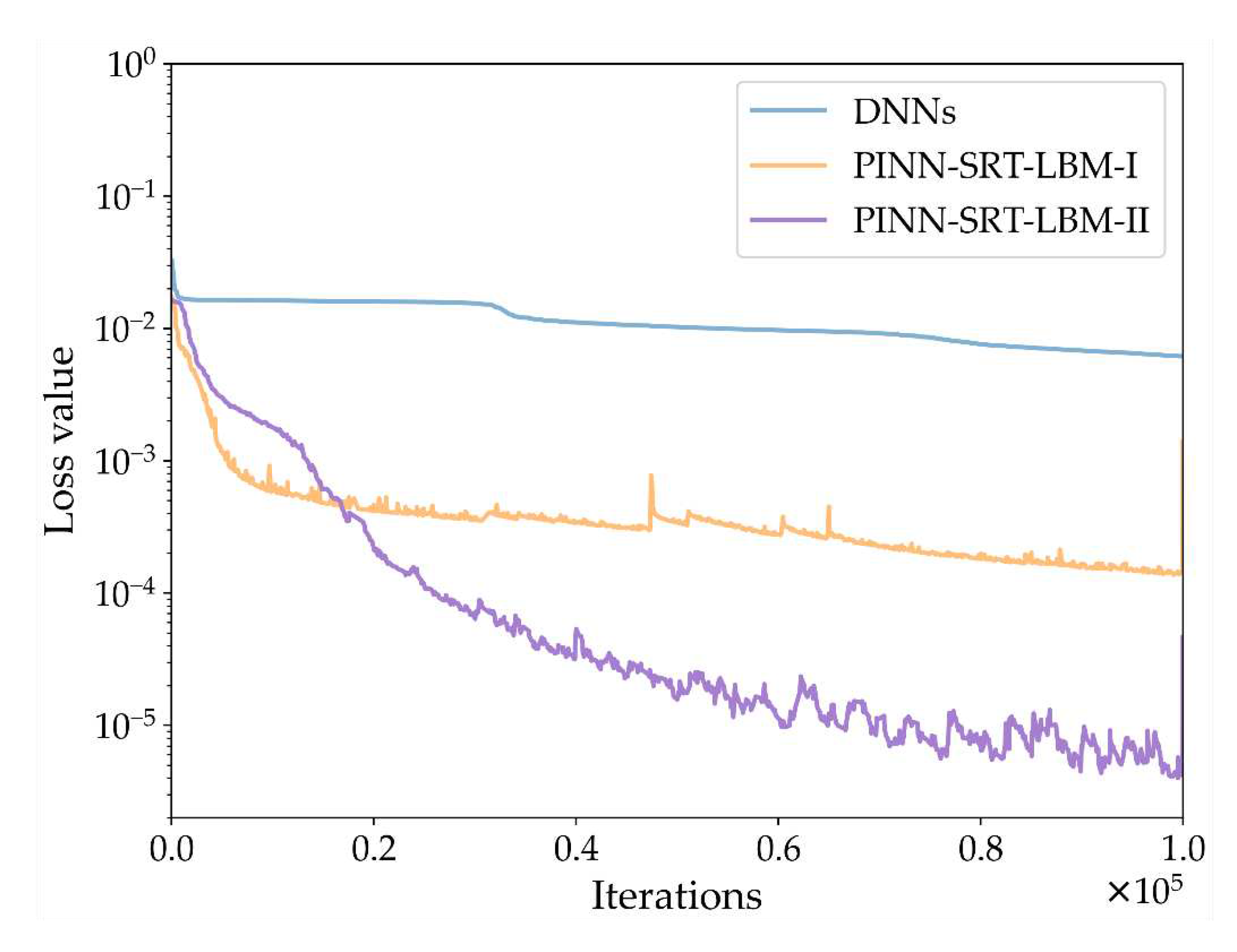
For the training settings, the foundational components DNN-I and DNN-II within the PINN-SRT-LBM-I and PINN-SRT-LBM-II were configured with 8 hidden layers, each containing 40 neurons and utilizing the tanh activation function. The DNNs employed for comparison were also designed with 8 hidden layers and 40 neurons per layer. The PINN-NS’s network configuration followed the default structure outlined in [25], which entails 6 layers with 40 neurons each, utilizing the tanh activation function. Regarding optimizer selection, DNNs were optimized using the SGD optimizer, while the other models employed a combination of the Adam optimizer and L-BFGS optimizer. The maximum number of iterations was uniformly set to 100,000.
Figure 16 presents a schematic of the variations in the training loss curves for the three models: DNNs, PINN-SRT-LBM-I, and PINN-SRT-LBM-II. From the trend of loss value shown in Figure 16, it can be concluded that the PINN-SRT-LBM-II model exhibits a more distinct convergence range when simulating the inverse problem of 2D flow around circular cylinder. This suggests that the precision of the PINN-SRT-LBM-II model is higher compared to the other models. Additionally, Table 6 presents the relative errors L2 for u and v at T=100.
Conclusions can be drawn from the relative errors L2 of the results by the four models presented in Table 6. Under the same training conditions, our proposed PINN-SRT-LBM-II model achieves a level of accuracy comparable to that of the PINN-NS model in [25]. Additionally, PINN-SRT-LBM-II outperforms PINN-SRT-LBM-I in simulating the inverse problem of 2D. Consequently, for the subsequent experiments, we will employ the PINN-SRT-LBM-II model.
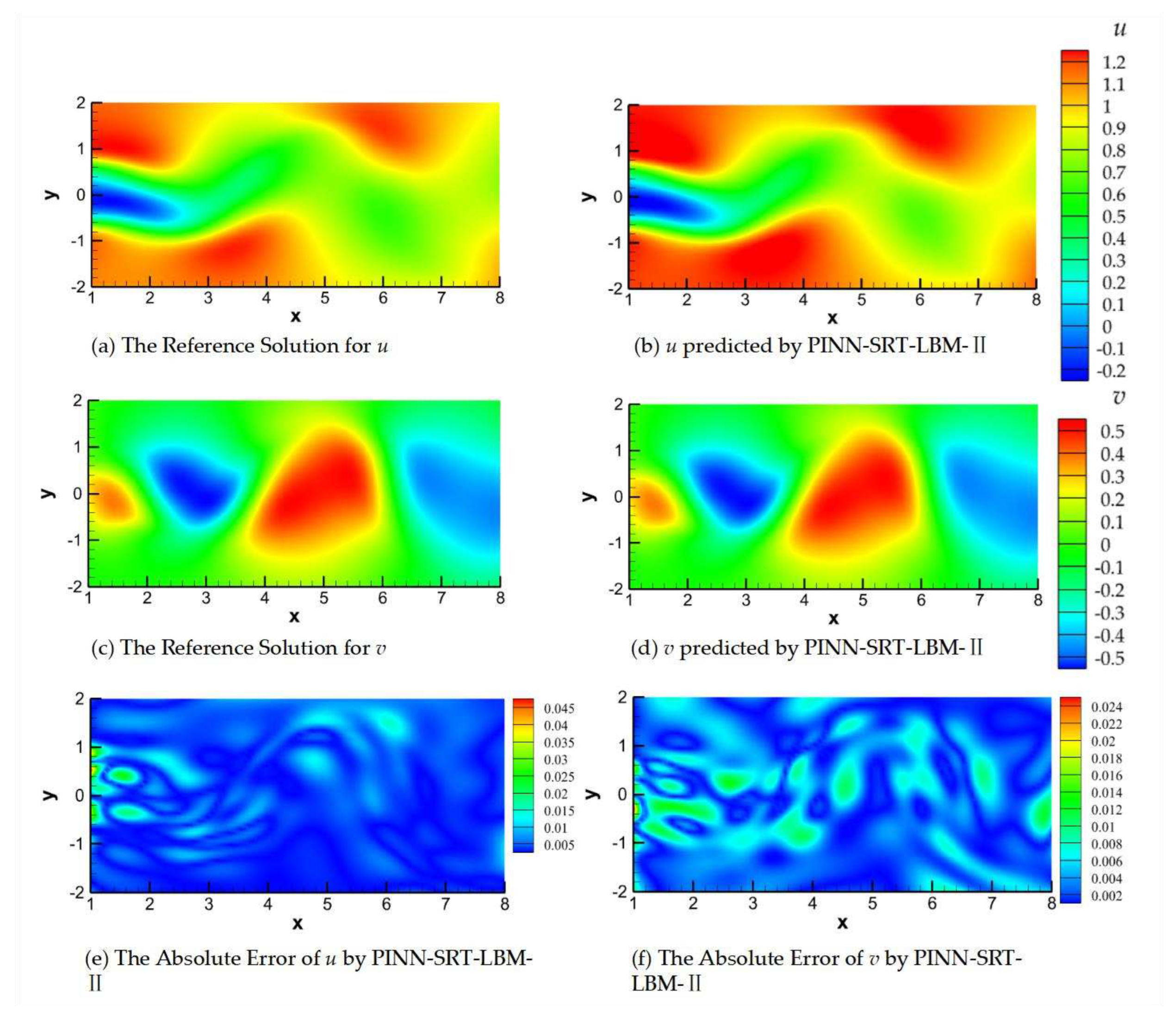
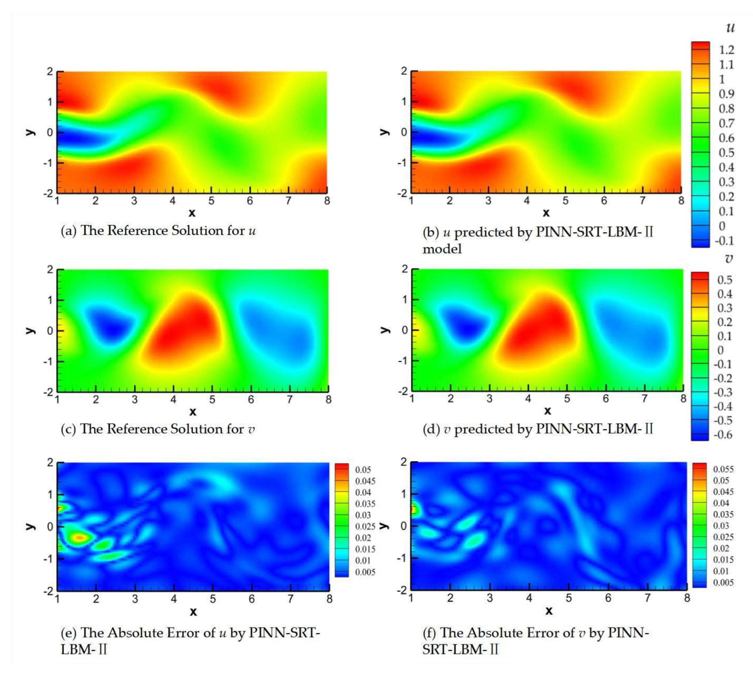
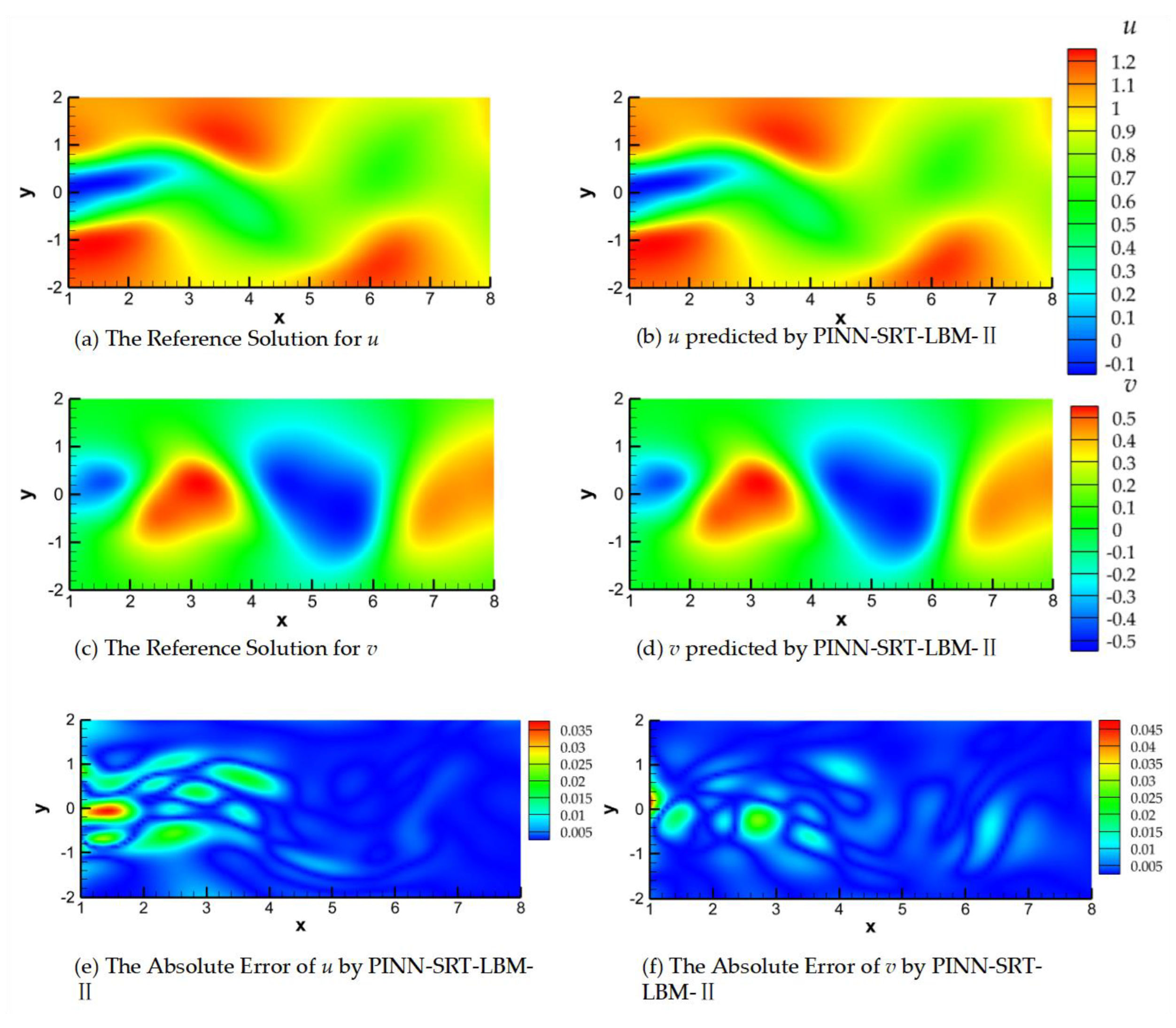
Flow around circular cylinder is a classic unsteady flow phenomenon. In this paper, an attempt is made to verify the learning effect of the PINN-SRT-LBM in the whole continuous time domain. Predictions using the PINN-SRT-LBM-II model were performed at T=50, 100, 200. Refer to Figure 17, Figure 18, and Figure 19for the respective results.
In Figure 17, Figure 18 and Figure 19, (a) and (b) represent the reference solution and model predictions for u (velocity component in the x-direction), (c) and (d) depict the reference solution and model predictions for v (velocity component in the y-direction), and (e) and (f) show the visualizations of the absolute errors for u and v, respectively.
Observing the absolute errors in panels (e) and (f) of Figure 17, Figure 18 and Figure 19 leads to a reasonable inference. Due to error accumulation, areas with larger absolute errors are predominantly located in regions of significant fluid variation, aligning well with the flow patterns in cylinder wake flow. The shedding of the Kármán vortex street in the wake exhibits the most pronounced variations, posing a challenge for neural networks to capture the underlying physical distribution patterns. This issue can potentially be addressed through alterations in training methodologies and optimization of neural network structures. Upon sequential comparison at time snapshots T=50, 100, and 200, a noteworthy observation emerges when focusing on the early time slice (T=50), as shown in Figure 17. Due to the absence of a relatively stable flow configuration and the periodic shedding of the Kármán vortex street, the PINN-SRT-LBM-II model's predictions exhibit oscillations in the distribution of absolute errors within the computational domain, owing to the abrupt variations in the underlying physical distribution patterns.
It is noteworthy that the absolute error values in the model predictions shown in Figure 17, Figure 18 and Figure 19 do not exceed magnitudes of 1×10⁻¹. Furthermore, the majority of the computational domain exhibits absolute errors in the model predictions that are smaller than 1×10⁻². From this, the conclusion can be drawn that the PINN-SRT-LBM-II model is capable of providing highly accurate prediction results across the continuous temporal and spatial domain of the unsteady 2D inverse problem.
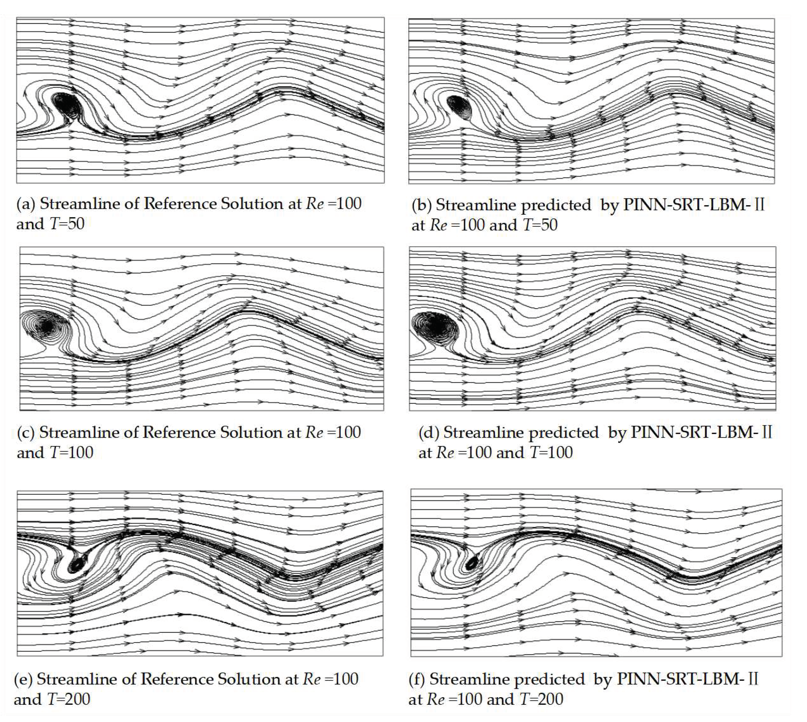
To validate the physical reliability of the prediction results generated by the PINN-SRT-LBM-II model, Figure 20 provides streamline diagrams for T=50, 100, 200. In Figure 20, panels (a) and (b) depict the streamline patterns of the reference solution and model predictions at T=50; panels (c) and (d) display the patterns at T=100; and panels (e) and (f) illustrate the patterns at T=200. By comparing the streamline patterns of the reference solution with those of the model predictions, it becomes apparent that the positions of vortex shedding are nearly identical. While the dataset only captures a portion of the wake, excluding the performance near the boundary, the congruence between vortex shedding positions and streamline patterns between the reference solution and the model predictions still underscores the physical reliability of the results obtained from the PINN-SRT-LBM-II model.
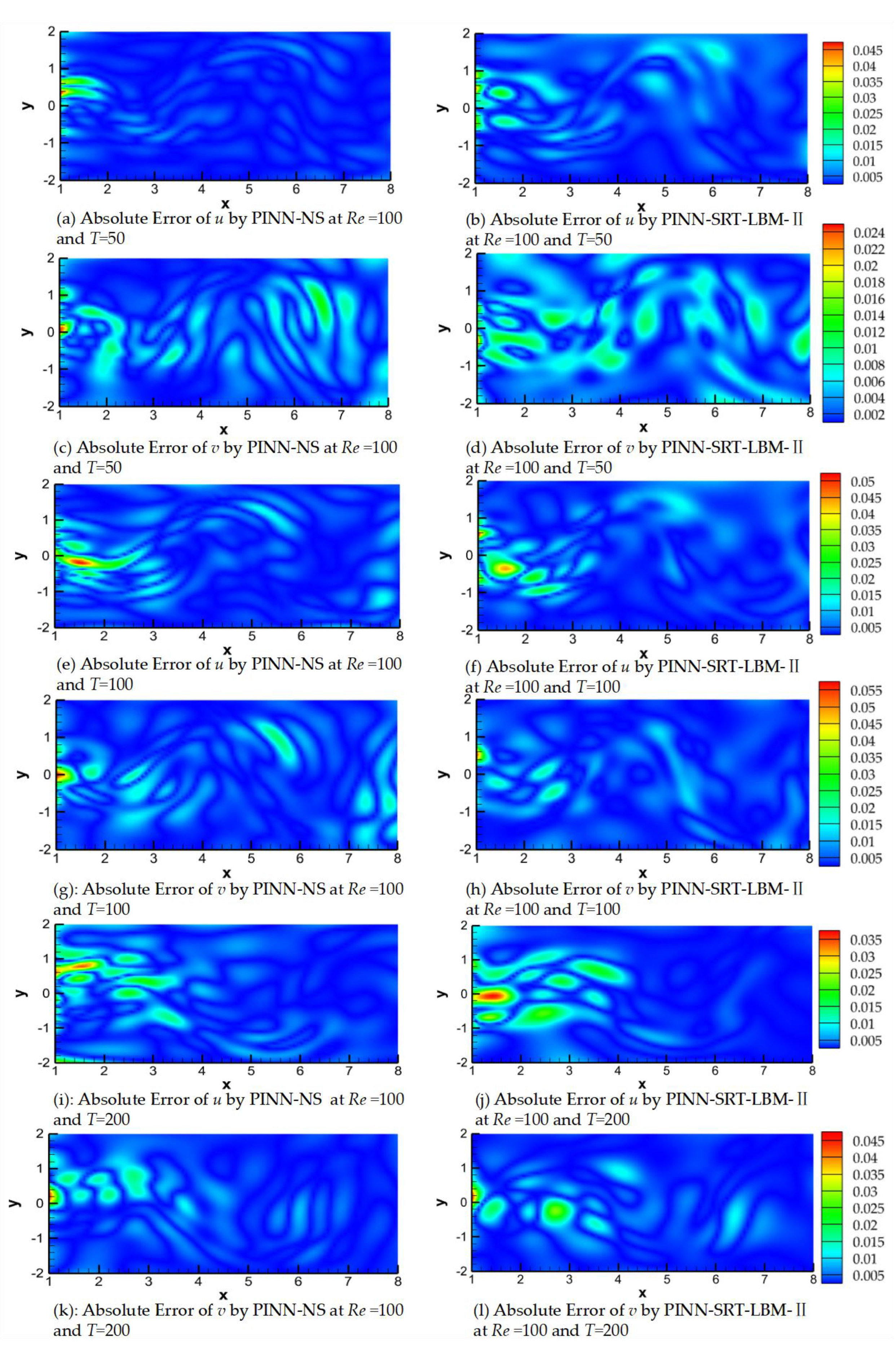
Finally, in Figure 21, we present the visualizations of the absolute errors for u and v, simulated by PINN-NS and PINN-SRT-LBM-II. From the visualizations, a reasonable deduction can be made that, under the same training parameter settings, the accuracy of the prediction results from PINN-SRT-LBM-II is comparable to that of PINN-NS. At the boundaries of the simulation region, the performance of PINN-SRT-LBM-II is better than PINN-NS. However, in regions characterized by more pronounced variations in physical behavior, the predictive accuracy of PINN-SRT-LBM-II is at a disadvantage. Overall, the accuracy of simulations conducted by the PINN-SRT-LBM-II model is approaching that of PINN-NS. This underscores the potential of mesoscopic physics methods in conjunction with PINNs except macroscopic physics methods and demonstrates the feasibility of employing mesoscopic physics methods combined with PINNs for simulating inverse problems in fluid mechanics.
In this part, this paper employed the PINN-SRT-LBM-II model to test its performance in simulating 2D unsteady fluid mechanics inverse problems. Moreover, for an impartial assessment of the PINN-SRT-LBM-II model's capabilities, we compared its prediction accuracy with that achieved by existing PINNs coupled with macroscopic physics methods, particularly the Navier-Stokes equations. The test data and comparative results collectively indicate the substantial potential of the PINN-SRT-LBM-II model in inverse problem simulations. Notably, in the realm of simulating 2D inverse problems in fluid mechanics, the performance of the PINN-SRT-LBM-II model has already reached the same level as that presented in reference [24], where PINNs were combined with the Navier-Stokes equations.
4. Conclusions

To solve the inverse problem in fluid mechanics, this paper proposes PINN-SRT-LBM by combining SRT-LBM with PINNs. The model proposed in this work has the capability of extracting the features of the flow to the constraints of the physical laws, and providing spatio-temporal simulation results. For the 1D problem, this paper proposes PINN-SRT-LBM-I and for the 2D problem this paper proposes PINN-SRT-LBM-II. The combination of SRT-LBM with deep neural networks is achieved by reducing the Mean Square Loss which consists of the physical residual values and the existing macroscopic quantities.
The comparison tests demonstrate that PINN-SRT-LBM-I has the advantages of high accuracy and stable prediction results in simulating the 1D inverse problem, and PINN-SRT-LBM-II has the advantages of high physical reliability in simulating the 2D inverse problem with the advantages of high accuracy. The two sub-models of PINN-SRT-LBM can flexibly solve complex inverse problems in fluid mechanics under different scenarios.
To further test the performance of the proposed model, this paper conducts comparisons of PINN-SRT-LBM with DNNs and PINN-NS, and the results show the scalability of PINN-SRT-LBM. The comparison experiments in different dimensions show that PINN-SRT-LBM is suitable for both unsteady and steady state flow simulations, showing excellent versatility.
The combination of PINNs and LBM can be used to solve the inverse problem in fluid mechanics, and the model proposed in this paper has good scalability and extensibility in different dimensions. In particular, the PINN-SRT-LBM is applicable to 1D and 2D unsteady flow and steady flow inverse problems. The potential of PINNs for inverse problems in fluid mechanics can be further developed in the future work by evaluating the neural network model or replacing the physical method.

Author Contributions

Conceptualization, Zhixiang Liu and Yuanji Chen; Data curation, Wei Song; Investigation, Ge Song and Wei Song; Methodology, Zhixiang Liu and Yuanji Chen; Project administration, Wei Song and Jingxiang Xu; Resources, Zhixiang Liu, Ge Song and Wei Song; Software, Zhixiang Liu and Yuanji Chen; Supervision, Ge Song, Wei Song and Jingxiang Xu; Validation, Zhixiang Liu and Yuanji Chen; Writing – original draft, Zhixiang Liu, Yuanji Chen and Wei Song; Writing – review & editing, Ge Song, Wei Song and Jingxiang Xu.

Funding

This research was funded by National Key Research and Development Program of China (Grant No.2021YFC3101601); National Natural Science Foundation of China (Grant No. 61972240) and the Program for the Capacity Development of Shanghai Local Colleges (Grant No. 20050501900).

Data Availability Statement

Experimental data related to this paper can be requested from the authors by email if any researcher in need of the dataset, email: zxliu@shou.edu.cn.

Acknowledgments

The authors would like to express their gratitude for the support of the Fishery Engineering and Equipment Innovation Team of Shanghai High-level Local University.

Conflicts of Interest

The authors declare no conflict of interest.

References

  1. Sharma, P.; Chung, W.T.; Akoush, B.; Ihme, M. A Review of Physics-Informed Machine Learning in Fluid Mechanics. Energies 2023, 16, 2343. [Google Scholar] [CrossRef]
  2. Mahony, N.O.; Campbell, S.; Carvalho, A.; Harapanahalli, S.; Velasco-Hernandez, G.; Krpalkova, L.; Riordan, D.; Walsh, J. Deep Learning vs. Traditional Computer Vision; 2020; Vol. 943.
  3. Liu, X.; He, P.; Chen, W.; Gao, J. Multi-Task Deep Neural Networks for Natural Language Understanding 2019.
  4. Nassif, A.B.; Shahin, I.; Attili, I.; Azzeh, M.; Shaalan, K. Speech Recognition Using Deep Neural Networks: A Systematic Review. IEEE access 2019, 7, 19143–19165. [Google Scholar] [CrossRef]
  5. Hu, C.; Cai, Z.; Zhang, Y.; Yan, R.; Cai, Y.; Cen, B. A Soft Actor-Critic Deep Reinforcement Learning Method for Multi-Timescale Coordinated Operation of Microgrids. Protection and Control of Modern Power Systems 2022, 7, 29. [Google Scholar] [CrossRef]
  6. Rawat, W.; Wang, Z. Deep Convolutional Neural Networks for Image Classification: A Comprehensive Review. Neural Computation 2017, 29, 2352–2449. [Google Scholar] [CrossRef]
  7. Ge, Z.; Liu, S.; Wang, F.; Li, Z.; Sun, J. YOLOX: Exceeding YOLO Series in 2021 2021.
  8. Yu, C.; Wang, J.; Peng, C.; Gao, C.; Yu, G.; Sang, N. BiSeNet: Bilateral Segmentation Network for Real-Time Semantic Segmentation.; 2018; pp. 325–341.
  9. Mikolov, T.; Le, Q.V.; Sutskever, I. Exploiting Similarities among Languages for Machine Translation 2013.
  10. Gardner, M.W.; Dorling, S.R. Artificial Neural Networks (the Multilayer Perceptron)—a Review of Applications in the Atmospheric Sciences. Atmospheric Environment 1998, 32, 2627–2636. [Google Scholar] [CrossRef]
  11. Gu, J.; Wang, Z.; Kuen, J.; Ma, L.; Shahroudy, A.; Shuai, B.; Liu, T.; Wang, X.; Wang, G.; Cai, J.; et al. Recent Advances in Convolutional Neural Networks. Pattern Recognition 2018, 77, 354–377. [Google Scholar] [CrossRef]
  12. Zaremba, W.; Sutskever, I.; Vinyals, O. Recurrent Neural Network Regularization 2015.
  13. Godunov, S.K.; Bohachevsky, I. Finite Difference Method for Numerical Computation of Discontinuous Solutions of the Equations of Fluid Dynamics. Matematičeskij sbornik 1959, 47(89), 271–306.
  14. Eymard, R.; Gallouët, T.; Herbin, R. Finite Volume Methods. In Handbook of Numerical Analysis; Solution of Equation in ℝ (Part 3), Techniques of Scientific Computing (Part 3); Elsevier, 2000; Vol. 7, pp. 713–1018.
  15. Zienkiewicz, O.C.; Taylor, R.L.; Zhu, J.Z. The Finite Element Method: Its Basis and Fundamentals; Elsevier, 2005; ISBN 978-0-08-047277-5.
  16. Canuto, C.; Hussaini, M.Y.; Quarteroni, A.; Zang, T.A. Spectral Methods: Evolution to Complex Geometries and Applications to Fluid Dynamics; Springer Science & Business Media, 2007; ISBN 978-3-540-30728-0.
  17. Hollingsworth, S.A.; Dror, R.O. Molecular Dynamics Simulation for All. Neuron 2018, 99, 1129–1143. [Google Scholar] [CrossRef]
  18. Wolfram, S. Cellular Automata as Models of Complexity. Nature 1984, 311, 419–424. [Google Scholar] [CrossRef]
  19. Chen, S.; Doolen, G.D. LATTICE BOLTZMANN METHOD FOR FLUID FLOWS. Annu. Rev. Fluid Mech. 1998, 30, 329–364. [Google Scholar] [CrossRef]
  20. Wang, M.; Pan, N. Predictions of Effective Physical Properties of Complex Multiphase Materials. Materials Science and Engineering: R: Reports 2008, 63, 1–30. [Google Scholar] [CrossRef]
  21. Körner, C.; Pohl, T.; Rüde, U.; Thürey, N.; Zeiser, T. Parallel Lattice Boltzmann Methods for CFD Applications. In Numerical Solution of Partial Differential Equations on Parallel Computers; Bruaset, A.M., Tveito, A., Eds.; Lecture Notes in Computational Science and Engineering; Springer-Verlag: Berlin/Heidelberg, 2006; Vol. 51, pp. 439–461. ISBN 978-3-540-29076-6. [Google Scholar]
  22. Chen, X.; Yang, G.; Yao, Q.; Nie, Z.; Jiang, Z. A Compressed Lattice Boltzmann Method Based on ConvLSTM and ResNet. Computers & Mathematics with Applications 2021, 97, 162–174. [Google Scholar] [CrossRef]
  23. Raissi, M.; Perdikaris, P.; Karniadakis, G.E. Physics-Informed Neural Networks: A Deep Learning Framework for Solving Forward and Inverse Problems Involving Nonlinear Partial Differential Equations. Journal of Computational Physics 2019, 378, 686–707. [Google Scholar] [CrossRef]
  24. Raissi, M.; Perdikaris, P.; Karniadakis, G.E. Physics Informed Deep Learning (Part I): Data-Driven Solutions of Nonlinear Partial Differential Equations. 2017. [CrossRef]
  25. Raissi, M.; Perdikaris, P.; Karniadakis, G.E. Physics Informed Deep Learning (Part II): Data-Driven Discovery of Nonlinear Partial Differential Equations. 2017. [CrossRef]
  26. Lou, Q.; Meng, X.; Karniadakis, G.E. Physics-Informed Neural Networks for Solving Forward and Inverse Flow Problems via the Boltzmann-BGK Formulation. Journal of Computational Physics 2021, 447, 110676. [Google Scholar] [CrossRef]
  27. Han, J.; Ma, C.; Ma, Z.; E, W. Uniformly Accurate Machine Learning-Based Hydrodynamic Models for Kinetic Equations. Proc. Natl. Acad. Sci. U.S.A. 2019, 116, 21983–21991. [Google Scholar] [CrossRef]
  28. Da Wang, Y.; Chung, T.; Armstrong, R.T.; Mostaghimi, P. ML-LBM: Machine Learning Aided Flow Simulation in Porous Media. 2020. [CrossRef]
  29. Shenoy, A.V.; Mashelkar, R.A. Thermal Convection in Non-Newtonian Fluids. In Advances in Heat Transfer; Elsevier, 1982; Vol. 15, pp. 143–225 ISBN 978-0-12-020015-3.
  30. Akkutlu, I.Y.; Efendiev, Y.; Vasilyeva, M.; Wang, Y. Multiscale Model Reduction for Shale Gas Transport in Poroelastic Fractured Media. Journal of Computational Physics 2018, 353, 356–376. [Google Scholar] [CrossRef]
  31. Jin, Z.; Firoozabadi, A. Flow of Methane in Shale Nanopores at Low and High Pressure by Molecular Dynamics Simulations. The Journal of chemical physics 2015, 143, 104315. [Google Scholar] [CrossRef]
  32. Redman, A.L.; Bailleres, H.; Perré, P.; Carr, E.; Turner, I. A Relevant and Robust Vacuum-Drying Model Applied to Hardwoods. Wood Sci Technol 2017, 51, 701–719. [Google Scholar] [CrossRef]
  33. Karniadakis, G.; Beskok, A.; Aluru, N. Microflows and Nanoflows: Fundamentals and Simulation; Springer Science & Business Media, 2006; ISBN 978-0-387-28676-1.
  34. Sallam, O.; Fürth, M. On the Use of Fourier Features-Physics Informed Neural Networks (FF-PINN) for Forward and Inverse Fluid Mechanics Problems. Proceedings of the Institution of Mechanical Engineers, Part M: Journal of Engineering for the Maritime Environment 2023, 147509022311664. [CrossRef]
  35. Jin, X.; Cai, S.; Li, H.; Karniadakis, G.E. NSFnets (Navier-Stokes Flow Nets): Physics-Informed Neural Networks for the Incompressible Navier-Stokes Equations. Journal of Computational Physics 2021, 426, 109951. [Google Scholar] [CrossRef]
  36. Mao, Z.; Jagtap, A.D.; Karniadakis, G.E. Physics-Informed Neural Networks for High-Speed Flows. Computer Methods in Applied Mechanics and Engineering 2020, 360, 112789. [Google Scholar] [CrossRef]
  37. Raissi, M.; Yazdani, A.; Karniadakis, G.E. Hidden Fluid Mechanics: Learning Velocity and Pressure Fields from Flow Visualizations. Science 2020, 367, 1026–1030. [Google Scholar] [CrossRef]
  38. Bhatnagar, P.L.; Gross, E.P.; Krook, M. A Model for Collision Processes in Gases. I. Small Amplitude Processes in Charged and Neutral One-Component Systems. Phys. Rev. 1954, 94, 511–525. [Google Scholar] [CrossRef]
  39. Qian, Y.H.; D’Humières, D.; Lallemand, P. Lattice BGK Models for Navier-Stokes Equation. Europhys. Lett. 1992, 17, 479–484. [Google Scholar] [CrossRef]
  40. (a)Glorot, X.; Bengio, Y. Understanding the Difficulty of Training Deep Feedforward Neural Networks. In Proceedings of the Proceedings of the Thirteenth International Conference on Artificial Intelligence and Statistics; JMLR Workshop and Conference Proceedings, March 31 2010; pp. 249–256.
  41. Toro, E.F. Riemann Solvers and Numerical Methods for Fluid Dynamics: A Practical Introduction; Springer Science & Business Media, 2013; ISBN 978-3-662-03490-3.
  42. Guo, Z.; Shu, C. Lattice Boltzmann Method And Its Application In Engineering; World Scientific, 2013; ISBN 978-981-4508-31-5.
  43. Sod, G.A. A Survey of Several Finite Difference Methods for Systems of Nonlinear Hyperbolic Conservation Laws. Journal of Computational Physics 1978, 27, 1–31. [Google Scholar] [CrossRef]
  44. Zhang, C.; Bengio, S.; Hardt, M.; Recht, B.; Vinyals, O. Understanding Deep Learning (Still) Requires Rethinking Generalization. Commun. ACM 2021, 64, 107–115. [Google Scholar] [CrossRef]
  45. Vanka, S.P. Block-Implicit Multigrid Solution of Navier-Stokes Equations in Primitive Variables. Journal of Computational Physics 1986, 65, 138–158. [Google Scholar] [CrossRef]
  46. Ghia, U.; Ghia, K.N.; Shin, C.T. High-Re Solutions for Incompressible Flow Using the Navier-Stokes Equations and a Multigrid Method. Journal of Computational Physics 1982, 48, 387–411. [Google Scholar] [CrossRef]
  47. Hou, S.; Zou, Q.; Chen, S.; Doolen, G.; Cogley, A.C. Simulation of Cavity Flow by the Lattice Boltzmann Method. Journal of Computational Physics 1995, 118, 329–347. [Google Scholar] [CrossRef]
  48. Karniadakis, G.; Sherwin, S.J. Spectral/Hp Element Methods for Computational Fluid Dynamics: Second Edition; OUP Oxford, 2005; ISBN 978-0-19-852869-2.
  49. Wille, R. Kármán Vortex Streets. In Advances in Applied Mechanics; Elsevier, 1960; Vol. 6, pp. 273–287 ISBN 978-0-12-002006-5.
Figure 1. DnQm discrete velocity model.
Preprints 84667 g001
Figure 2. PINN-SRT-LBM-I model.
Preprints 84667 g002
Figure 3. PINN-SRT-LBM-II model.
Preprints 84667 g003
Figure 4. The reference solution structure of lid-driven cavity flow.
Preprints 84667 g004
Figure 5. Training loss curves of PINN-SRT-LBM-I, PINN-SRT-LBM-II, and DNNs.
Preprints 84667 g005
Figure 6. Training loss curves of PINN-SRT-LBM-I.
Preprints 84667 g006
Figure 7. Comparison between the predicted results of the PINN-SRT-LBM-I model and the exact solution.
Preprints 84667 g007
Figure 8. Comparison of the training loss curves for DNNs, PINN-SRT-LBM-I, and PINN-SRT-LBM-II at Re = 1000.
Preprints 84667 g008
Figure 9. Comparison of the absolute error for PINN-SRT-LBM-I, PINN-SRT-LBM-II, DNNs and the reference solution at Re = 1000 and T = 100.
Preprints 84667 g009
Figure 10. Training loss curves at Re = 400,1000,2000,5000.
Preprints 84667 g010
Figure 11. Comparison of the reference solution, the predictions from PINN-SRT-LBM-II, and the absolute errors at Re = 5000 and T = 100.
Preprints 84667 g011
Figure 12. Comparison of the reference solution, the predictions from PINN-SRT-LBM-II, and the absolute errors at Re = 400 and T = 100.
Preprints 84667 g012
Figure 13. Comparison of the reference solution, the predictions from PINN-SRT-LBM-II, and the absolute errors at Re =1000 and T=100.
Preprints 84667 g013
Figure 14. Comparison of the reference solution, the predictions from PINN-SRT-LBM-II, and the absolute errors at Re =1000 and T=200.
Preprints 84667 g014
Figure 15. Data acquisition region.
Preprints 84667 g015
Figure 16. The training loss curves for DNNs, PINN-SRT-LBM-I, PINN-SRT-LBM-II at Re = 100 and T =100.
Preprints 84667 g016
Figure 17. The reference solution, the predictions from PINN-SRT-LBM-II, and the absolute errors at Re = 100 and T=50.
Preprints 84667 g017
Figure 18. The reference solution, the predictions from PINN-SRT-LBM-II, and the absolute errors at Re = 100 and T=100.
Preprints 84667 g018
Figure 19. The reference solution, the predictions from PINN-SRT-LBM-II, and the absolute errors at Re = 100 and T=200.
Preprints 84667 g019
Figure 20. Streamline traces of the reference solution and the predictions from the PINN-SRT-LBM-II model at Re = 100, T = 50, 100, 200.
Preprints 84667 g020
Figure 21. Comparison of the absolute errors for PINN-NS and PINN-SRT-LBM-II.
Preprints 84667 g021
Table 1. Dataset structure.
Dataset Xexact ρexact Uexact T
Sod shock tube Ns×D1 Ns×Ts Ns×D1×Ts Ts
Lid-driven cavity flow NL×D2 NL×TL NL×D2×TL TL
Flow around circular cylinder Ncy×D2 Ncy×Tcy Ncy×D2×Tcy Tcy
Table 2. The relative errors L2 for PINN-SRT-LBM-I, PINN-SRT-LBM-II, and DNNs.
Model erru(%) errp(%) errρ(%)
PINN-SRT-LBM-I
PINN-SRT-LBM-II
6.47%
15.87%
1.64%
10.56%
1.85%
14.87%
DNNs 18.87% 5.66% 5.75%
Table 3. The relative errors L2 for PINN-SRT-LBM-I, PINN-SRT-LBM-II, and DNNs at Re = 1000 and T=100.
Model erru(%) errv(%) errρ(%)
DNNs 2.01% 1.76% 0.23%
PINN-SRT-LBM-I
PINN-SRT-LBM-II
0.30%
0.08%
0.26%
0.06%
0.05%
0.03%
Table 4. Comparison between the predicted center coordinates of the primary vortex by the PINN-SRT-LBM-II model and the reference results.
Re A B C D
400 (0.5563,0.6000) (0.5547,0.6055) (0.5608,0.6078) (0.5556,0.6000)
1000 (0.5438,0.5625) (0.5313,0.5625) (0.5333,0.5647) (0.5327,0.5652)
2000 (0.5226,0.5482) (0.5255,0.5490) (0.5250,0.5500) (0.5254,0.5499)
5000 (0.5125,0.5313) (0.5117,0.5352) (0.5176,0.5373) (0.5137,0.5424)
Table 5. The relative errors L2 for PINN-SRT-LBM-II at Re=400, 1000, 2000, 5000.
Re erru(%) errv(%) errρ(%)
400
1000
2000
0.06%
0.08%
0.09%
0.09%
0.06%
0.06%
0.05%
0.04%
0.04%
5000 0.13% 0.05% 0.04%
Table 6. The relative error L2 at T=100.
Model erru(%) errv(%)
DNNs 13.48% 20.51%
PINN-SRT-LBM-I 2.71% 2.47%
PINN-SRT-LBM-II 0.49% 0.51%
PINN-NS 0.35% 0.72%
Disclaimer/Publisher’s Note: The statements, opinions and data contained in all publications are solely those of the individual author(s) and contributor(s) and not of MDPI and/or the editor(s). MDPI and/or the editor(s) disclaim responsibility for any injury to people or property resulting from any ideas, methods, instructions or products referred to in the content.
Copyright: This open access article is published under a Creative Commons CC BY 4.0 license, which permit the free download, distribution, and reuse, provided that the author and preprint are cited in any reuse.
Prerpints.org logo

Preprints.org is a free preprint server supported by MDPI in Basel, Switzerland.

Subscribe

© 2024 MDPI (Basel, Switzerland) unless otherwise stated