1. Introduction
In the operating lifetime of mechanical systems working at high dynamics, vibrations are a common source of fatigue damage that could lead components to premature failure. To test whether the components could withstand the elastodynamic loads occurring for a particular application, just the latter is used to tailor qualification tests performed by means of shakers/slip tables. The so -<called Test Tailoring procedure aims at a proper definition of the vibratory profiles (Mission Synthesis) to be used as the excitation for the device under test (DUT), based on the processing of reference environmental data – measured in those working conditions that are particularly significant to represent real-life excitations expected for the DUT – in order to reproduce their most important characteristics in laboratory tests.
Instead of replicating the recorded environmental data as shaker input signals, which would result in the major drawback of losing stochasticity and limiting the qualification tests to represent a given working condition only [
1], the conventional Mission Synthesis procedures implemented so far [
2] provide the synthesis of a test profile in terms of a Power Spectral Density (
PSD). In Random Control tests, the shaker controller then generates the actual vibration after applying the Inverse Fast Fourier Transform (
IFFT) to the spectral domain. Amplitudes and phases characterize this domain, with the former being obtained from the
PSD and the latter being randomly generated as uniformly distributed random variables.
Owing to their random generation, the probability distribution of the values of the obtained time-series is Gaussian. This could compromise the reliability of tests since most excitation signals encountered in real applications feature non-Gaussian distributions. A parameter that accounts for deviations from Gaussianity is
kurtosis [
3]: for Gaussian signals, its theoretical value amounts to 3.0, whereas if peaks and bursts or deterministic components are preponderant, it becomes higher or lower than 3.0, respectively. Signals with kurtosis value greater than 3.0 are named Leptokurtic, and so is their distribution.
Over the last decades, the so-called
kurtosis control methods have gained increasing interest: the aim is to generate shaker input signals by controlling both the
PSD and the kurtosis parameter, in order to carry out more realistic tests by preserving the nature of real-life random excitations (i.e. the values probability distribution due to peaks and bursts). Several kurtosis-control algorithms can be found in the literature [1, 4-17], which are essentially based on three different main approaches (or their possible combinations): Phase Manipulation [5, 8, 12, 16, 17], Amplitude Modulation [10, 11], and Polynomial Transformation [13-15]. The methods proposed feature different characteristics and performance depending on the corresponding targeted goals (not limited to durability testing applications, which is instead the general framework of the present work). Overall, however, one common critical issue exists that needs to be addressed by any procedure of kurtosis-control, as it significantly affects the effectiveness of transferring peaks and bursts from the excited base to the DUT. In fact, it is known that the response of a lightly damped system to a generic excitation may tend to a Gaussian probability distribution due to a filtering effect [
18]. Thus, if this occurs, the tests would be no different from the standard procedure that generates directly Gaussian signals. Hereinafter, this filtering effect will be referred to as
Papoulis’ Rule, which stems from the mathematician who proved it based on the
Central Limit Theorem [18, 19].
In this work, two novel algorithms are proposed for the synthesis of random excitation signals with prescribed
PSD and kurtosis value, able to robustly circumvent the Papoulis’ Rule and to excite a generic DUT effectively irrespective of the signal features of the reference environmental data. Indeed, most kurtosis control algorithms prove to be effective only if certain conditions are met (e.g.: the DUT natural frequencies must be known; the reference environmental data to be processed need to be narrowband signals…). The main difference between the two algorithms regards the predicted kurtosis value of the DUT response: constant and equal to the excitation one for the first algorithm, variable and significantly larger for the second one. Moreover, it will also be shown that the proposed methods can be used for accelerated fatigue-life tests with the help of the filter proposed by Kihm
et al. [
20]. These tests seek to preserve the damage potential of a signal measured from an application and replicate it in a shorter time. The damage potential associated with a vibratory excitation is estimated via a spectral function called Fatigue Damage Spectrum (
FDS) [
21] and current procedures already available in some commercial software permit the synthesis of a
PSD from prescribed
FDS and duration of the test [
2]. Since the output is the only
PSD, the standard procedure leads to accelerated tests featuring Gaussian excitation signals, hence the same problems with not preserving the nature of reference signals – possibly non-Gaussian – may occur in this case as well. The two kurtosis-control algorithms do not directly control the
FDS, but by convolving the synthesized signal with the filter mentioned above, it is possible to match a prescribed
FDS for accelerated fatigue-life tests while preserving the non-Gaussian features of the environmental data.
The paper structure is as follows:
Section 2 reports the theoretical background on the popular procedures of kurtosis-control and the analytical formulations of the two original algorithms proposed in this work; the results of the application of the algorithms for a case study are reported and discussed in
Section 3 and
Section 4, respectively; finally,
Section 5 is devoted to some concluding remarks. In addition, details about some computational issues related to the algorithms implementation are reported in the
Appendices: in particular, computationally efficient procedures for the implementation of kurtosis-control algorithms based on Phase Modulation and for the kurtosis value computation of multiple/concatenated time-series are proposed in
Appendix A and
Appendix B, respectively, whereas the effectiveness of the special filter proposed by Kihm
et al. in [
20] is analytically proven in
Appendix C.
2. Materials and Methods
2.1. Theoretical background
In the field of random vibration testing, the shaker controller typically generates a stationary vibratory signal in the time domain from a prescribed
PSD input by applying the
IFFT to the spectral domain. Amplitudes and phases characterize the spectral domain; the former are related to the
PSD via the equation:
where the amplitude
An of the
nth harmonic is related to the
nth PSD element
Gn and frequency resolution Δ
f. The randomness required for the generation of the time-series is guaranteed by the phases, which are defined as uniformly distributed random variables in the interval [0, 2π[. The time histories generated in such a way are always characterized by a probability distribution of their values close to Gaussian. The statistical parameter known as kurtosis is the 4
th statistical central moment of a signal, normalized by the 4
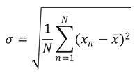
th power of its standard deviation. For Gaussian signals, the theoretical value of kurtosis is 3.0, whereas Leptokurtic signals feature greater values (e.g. due to high peaks caused by micro-collisions). In practical applications, discretized formulations of the signal statistical quantities are typically used:
where , σ, σ2, k are the mean value, the standard deviation, the variance, and the kurtosis of the signal, respectively, xn its nth sample, and N its total number of samples. Current kurtosis control algorithms are generally based on three approaches: Phase Manipulation (PM), Polynomial Transformation (PT), and Amplitude Modulation (AM).
PM methods [5, 8, 12, 16, 17] employ the formulation of kurtosis written in terms of the amplitudes and phases of a time-series. Steinwolf
et al. [4-9, 17] described some analytical methods that control kurtosis by changing only the phases while keeping the amplitudes constant. This would imply preserving the
PSD as well since it only depends on amplitudes. In
Appendix A, computational cost issues are discussed and an original procedure is proposed to efficiently implement the PM algorithms based on Steinwolf’s studies.
PT methods consist of generating a Gaussian signal
x(
t) with the prescribed
PSD first and then applying an analytical transformation of the form:
with the coefficients α
1 and α
3 being functions of the target kurtosis value [13-15]. The transformation in Eq. (6) presents two disadvantages: (
i) the
PSD of the signal is affected by an unwanted disturbance and (
ii) Papoulis’ Rule is very likely to occur, thus causing the peaks present in the input signal to be filtered out and leading the response to approaching a Gaussian probability distribution.
The second problem is similar to the case of PM methods. In fact, the effectiveness of kurtosis-control methods lies in the fact that the bursts of the signal must have either of two characteristics: (i) a long enough duration in order to appear also in the unavoidably time-delayed response of the system, (ii) a narrow-band frequency content containing the natural frequency of the system. Typically, the bursts generated by both PM and PT methods do not have a long enough duration and this is the reason why they are likely to be filtered out by the system.
Methods that generate bursts of desired duration employ the AM approach, which consists in modulating a Gaussian signal
x(
t) having the desired
PSD with an appropriate function
w(
t) in order to obtain a signal with a desired kurtosis value [10, 11]:
This method is effective in transferring the kurtosis value to the response of the DUT if the signal bursts of the modulating signal have greater duration than the inverse of the bandwidth of the lightly-damped system [
11]. The carrier waveform
w(
t) introduces low frequency components in the spectrum of
y(
t) compared to that of
x(
t), albeit negligible if
w(
t) is appropriately designed.
Both the algorithms presented in this paper, which aim to synthesize vibratory profiles whose kurtosis and PSD match the reference input ones, are based on two different approaches that can hardly be classified into the above-mentioned categories. The following Sections are devoted to the detailed description of their implementation.
2.2. Multi-Level Variance (MLV) algorithm
The algorithm named Multi-Level Variance (
MLV) attains the synthesis of a signal by dividing the signal duration
Ttot into
nb blocks of the same size and duration
Tb (
Tb =
Ttot/
nb). The generated blocks are not overlapped and have different variance, which is closely related to a modulation procedure, although no modulating function is explicitly used. As shown in the following, the different levels of variance
σi2 (
i = 1,…,
nb) are produced in such a way that the synthesized signal complies with the kurtosis and
PSD constraints. In general, the
PSD of a signal is computed by calculating the Fast Fourier Transforms (FFT) over small-sized blocks and squaring their magnitude to obtain the so-called periodograms. More specifically, the periodogram could be thought of as some sort of
PSD computed only for the generic block of the signal. After obtaining the periodograms, the last step is to average them in order to calculate the
PSD of the signal. In the algorithm, the
PSD of the
ith block of the signal,
Gi, is defined to be proportional to the
PSD of the reference signal,
G, as in the following expression:
In Eq. (8)
σtot2 and
σi2 are the variance values of the overall signal and the
ith block, respectively. It is to be highlighted that the
σi2 parameters are the unknowns, whereas
σtot2 can be calculated from either the reference signal, Eq. (4), or directly from the reference
PSD:
where
G(
f) is the
PSD amplitude at the generic frequency
f of a continuous signal. However, since the processed signal is discrete in practice, the
PSD is also discrete and the theoretical computation of Eq. (9) must be discretized. The unknown parameters
σi2 are also related to the overall variance
σtot2 through the following equation (cf.
Appendix B for proof):
From Eqs. (8, 10) the following relation must hold:
Since the
PSD G is computed by averaging the
PSDs of the blocks, Eq. (11) is automatically satisfied. Hence, the constraint on the
PSD spectrum is fulfilled if
nb values
σi2 that comply with Eq. (10) are found. In addition to Eqs. (10, 11), there is also a relation between the kurtosis values of the overall signal,
ktot, and of the single blocks,
ki (cf.
Appendix B):
The first step of the algorithm is to randomly generate the
σi2 values such that
σi2 ∈ [
σmin2,
σmax2] and
σmin2 <
σtot2 <
σmax2. The ratio
rσ2 =
σmin2/
σtot2 ∈ ]0, 1[ must be selected by the user as an input for the algorithm: the closer to 0, the more the variance of the synthesized signal will vary in time, whereas the opposite is true if closer to 1. The parameter
σmax2 is not selectable directly by the user because it is adjusted throughout the algorithm iterations in order to converge to the target kurtosis value. The user can also choose the number of bursts with high amplitude excursion of the synthesized signal (parameter
np = 0,…,
nb); this is typically done by referring to the number of bursts that can be observed in the reference measured data. The algorithm generates
np blocks with a variance equal to
σmax2, which is greater than the variance of the other blocks. The kurtosis
ki and variance
σi2 of the blocks are calculated via Eqs. (4, 5) only on the first iteration, whereas the discrete signal
xn is obtained by the
IFFT of the
PSD of the single blocks with randomly generated phases and then by concatenating the blocks. A random integer
s, representing a single block, is then automatically generated in the interval [1,
nb]. After the
σi2 levels are generated (
i = 1,…,
nb,
i ≠
s), the variance and the kurtosis of the randomly selected
sth block are calculated via the following relations, which stem from Eqs. (9, 12):
Eqs. (13, 14) are used in order to verify if the prescribed
PSD and target kurtosis can be achieved: indeed,
σs2 is required to be not null and
ks greater than a lower threshold,
ks_min, and smaller than an upper threshold,
ks_max. The upper threshold should not be set excessively high because it would lead to generating unrealistic peaks in the
sth block exceeding by far the amplitude of those of the other blocks. Afterward, in order to obtain the
ks given by Eq. (14), the harmonics phases of the
sth block are adjusted using a phase manipulation procedure (cf.
Section 2). With very few iterations, where the parameter
σmax2 is changed in order to converge towards the target kurtosis value, Eqs. (13, 14) are usually satisfied. The final step of the algorithm is to concatenate the generated blocks by smoothing them through proper interpolation of the values close to the edges of the adjoining blocks, in order to avoid unrealistic discontinuities among them.
In conclusion, the user has to insert:
the reference input signal or, alternatively, reference PSD and kurtosis value;
the duration Ttot of the signal to be synthesized;
the sampling frequency Fs of the synthesized signal (usually the same as the reference signal);
the signal blocks duration Tb;
the ratio rσ2;
the number of bursts np;
the lower and upper thresholds for kurtosis value ks_min and ks_max, respectively.
2.3. Variable Spectral Density (VSD) algorithm
The algorithm hereinafter called Variable Spectral Density (VSD) splits the signal to be synthesized into nb blocks of the same duration Tb as the previous algorithm. The major difference is that the PSD Gi of the ith block is randomly generated.
Let the
PSD matrix [
G’’ij] be defined as:
where
Nh is the number of spectral lines. This matrix has
Nh rows and
nb columns, with the
jth column being the
PSD vector of the
jth block of the reference signal. Eq. (15), where all the columns have the same elements (harmonic amplitudes), refers implicitly to a signal having a stationary
PSD. On the other hand, the
PSD matrix [
G’’ij] corresponding to the signal synthesized through the
MLV algorithm has the following form:
Both the matrices in Eqs. (15) and (16) satisfy Eq. (11) that may be rewritten in this case, in conformity with the notation used in this Section, as:
The
VSD algorithm synthesizes a signal with a
PSD variable over time, corresponding to a
PSD matrix having the most general form:
where the elements must comply with Eq. (17).
The generic matrix in Eq. (18) can be derived from Eqs. (15) and (17), by changing one row, the
ith for instance, as in the following equation, where
p ∈ [0, 1] and
l is a positive integer such that
l ≤
nb:
Equation (17) is still complied with if the terms of the type pGi are l – 1. If similar operations were done not only on the term Gij but also on other terms and in a random manner, then the PSD of each block could be varied still preserving the overall PSD.
In conclusion, the user is required to perform the following operations:
insert a reference input signal or, alternatively, reference PSD and kurtosis value;
set the duration Ttot and the sampling frequency Fs of the signal to be synthesized;
choose p ∈ [0, 1].
Then, the workflow of the algorithm is based on the following operations that are automatically performed:
set Tb and i = 1;
set s = 0;
choose a random element j of the ith row;
generate a positive random integer l ≤ nb – s;
set Gij = [1 + (l – 1)(1 – p)Gi and s = s + l;
repeat 3 – 4 – 5 with another value for j (different from the values generated in the previous loops) and another value of l, until s ≥ nb – 1;
set Gim = pGi with m ranging over all the elements of the ith row which have not been modified in point 5;
if i < Nh, set i = i+1 and repeat from point 2, otherwise proceed to point 9;
terminate if the kurtosis of the synthesized signal matches the target value (within a certain tolerance, to be preliminarily set), otherwise repeat from point 1 where a different Tb is automatically generated. Decreasing Tb makes the kurtosis value increase and vice versa (this is how the algorithm converges towards the target kurtosis).
As in the case of the MLV algorithm, the very last step is to smooth the signal at the edges of the blocks in order to avoid unrealistic discontinuities.
It is worth noting that a limitation of the algorithm could be that the variation of the PSD over time (i.e. over the blocks) is not controlled but randomly generated.
3. Results
Real field data sampled at 8192Hz and having a duration of 660s are used as reference signal for an example of application (
Figure 1). The synthesis by the
MLV and
VSD algorithms was performed in order to obtain signals with the same sampling frequency and duration for the sake of a direct and more straightforward comparison. Two signals synthesized by the
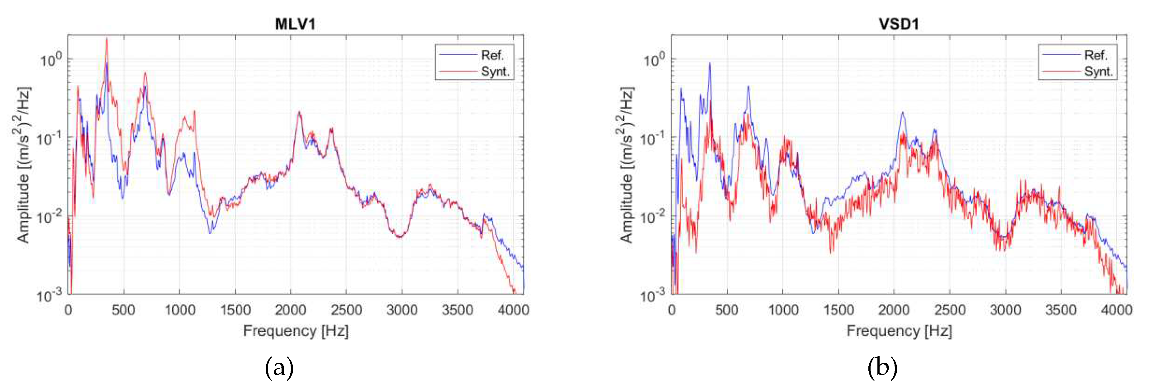
MLV algorithm are shown in
Figure 2, hereinafter referred to as MLV1 and MLV2, respectively. The main difference between the two implementations of the algorithm was in the choice of the signal blocks durations and number of bursts: {
Tb = 3s,
np = 10} and {
Tb = 0.1s,
np = 300}, for MLV1 and MLV2 signals, respectively. The parameter
rσ2 was set equal to 0.25 for both. Statistical parameters and
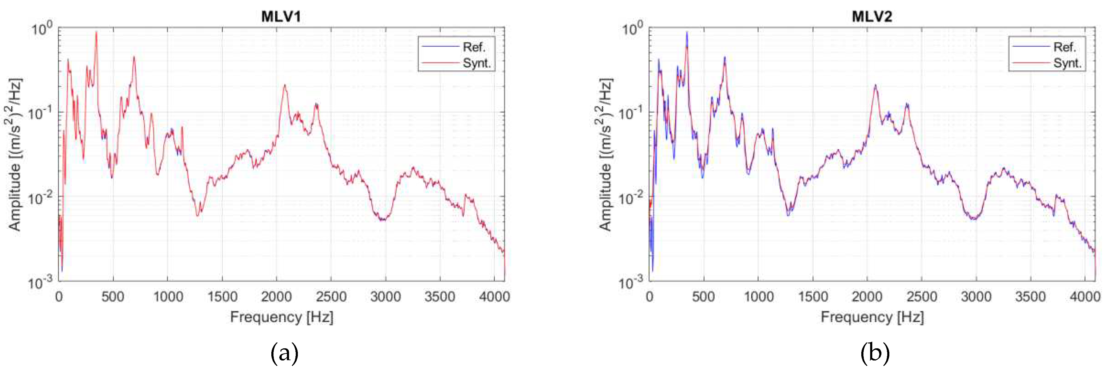
PSDs of the signals are respectively reported in
Table 1 and
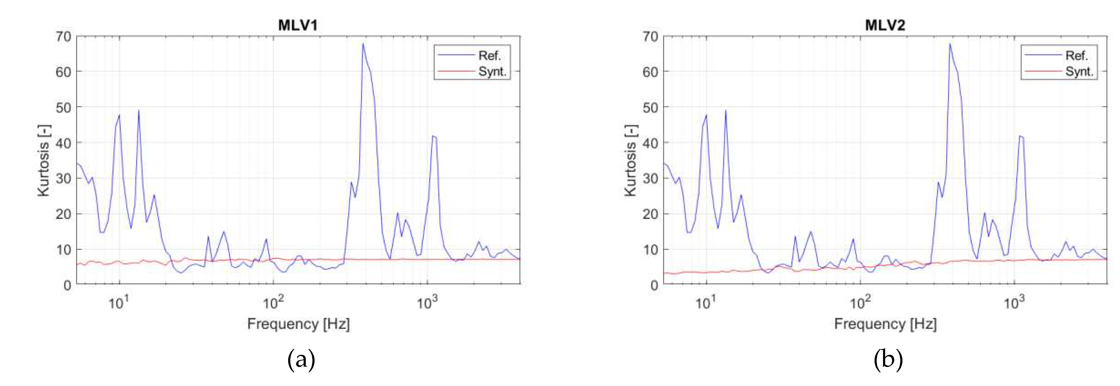
Figure 3, over the frequency range 0÷4096Hz. The acceleration response of a series of single-degree-of-freedom (SDOF) linear systems, with natural frequency in the range 0÷4000Hz and a constant damping ratio equal to 2.5%, was calculated by convolution between the impulse response of the system and its input. The response kurtosis of the synthesized and reference signals is shown in
Figure 4, where the kurtosis parameter is plotted versus the natural frequencies of the SDOF systems. It can be observed that the kurtosis of the synthesized signals remains approximately constant over the frequency range; however, the signal with the lower
Tb (MLV2) suffers more from the Papoulis’ Rule, whereas the higher
Tb (MLV1) permits the generation of bursts that last enough to be transferred to the response, thus almost preserving the input kurtosis value. By inspecting the plot, it should be evident that the kurtosis of the response to the reference signal is not constant over the frequency range and in particular, for some frequencies it is much higher.
The
VSD algorithm only requires the parameter
p to be specified, and two synthesized signals with different
p (respectively 0.1 and 0.6) are shown in
Figure 5, hereinafter referred to as VSD1 and VSD2, respectively. Their corresponding statistical parameters are listed in
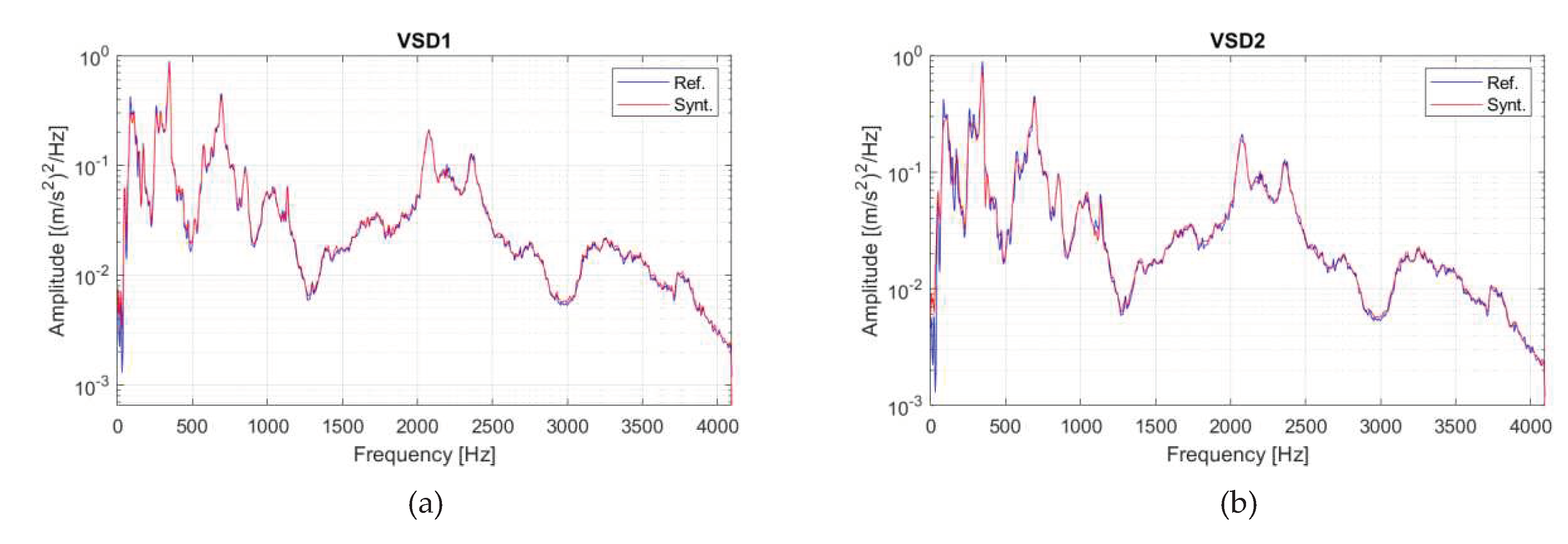
Table 2 and their
PSD in
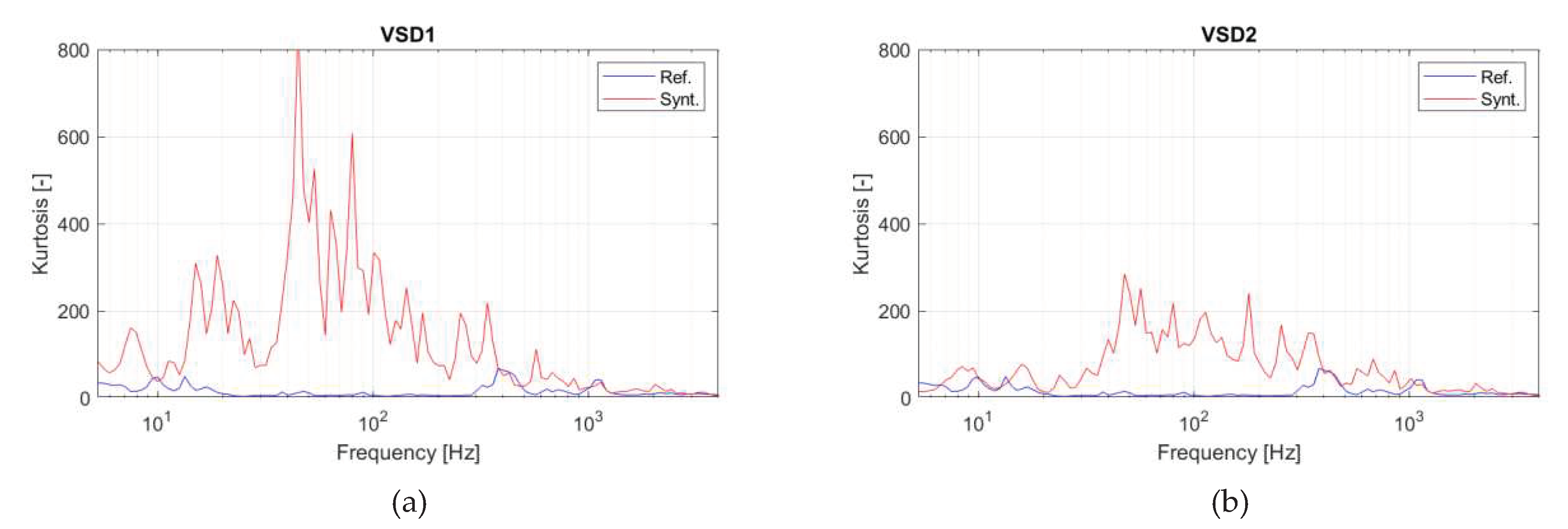
Figure 6. The kurtosis of the SDOF systems responses is shown in
Figure 7. It can be observed that the kurtosis changes over the frequency range and proves significantly higher than the input kurtosis, to which extent depending on parameter
p: the lower
p, the higher the output kurtosis.
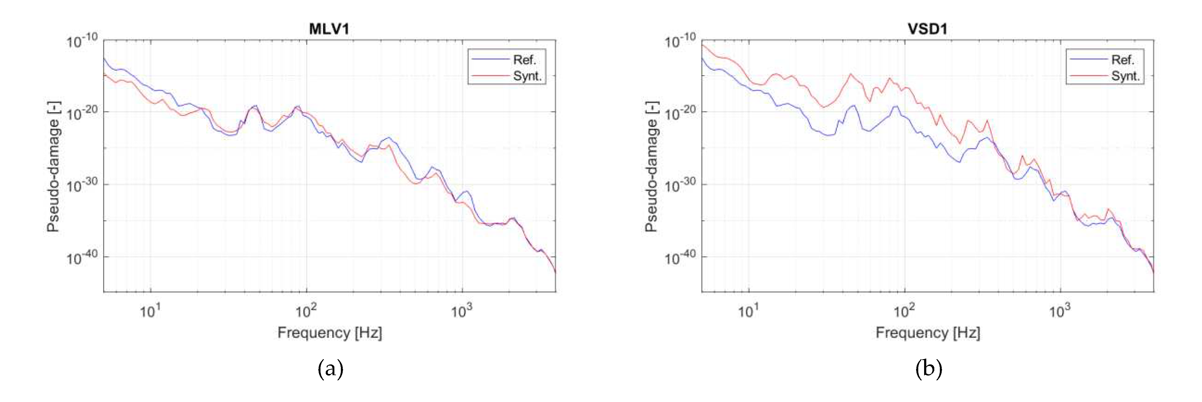
In the perspective of using the proposed algorithms to generate shaker input signals for fatigue life tests, further processing of the synthesized signals is carried out. For a straightforward comparative illustration of results, the duration of the hypothetical durability tests is ideally assumed to be equal to the duration of the reference field data. In particular, the
FDS curves over the frequency range 0÷4000Hz are calculated and plotted with a resolution of 1/12
th octave. For brevity, only the
FDS of the reference, MLV1, and VSD1 signals are shown. The most influent parameters in the
FDS calculation are the Wohler’s curve slope (i.e. the exponent
b in the well-known Basquin’s law
NSb = const.) and the damping ratio of the SDOF systems, which were set to 7 and 2.5%, respectively. The plots of the reference and the synthesized signals
FDSs are reported in
Figure 8. It should be evident that the Fatigue Damage curves are not overlapped. In order to adjust the
FDS of the signals to match the reference one, the filter described in [
20] is used (cf.
Appendix C for an original mathematical proof of the filter effectiveness). The steps of the procedure are:
calculate the FDSs of the reference and synthesized signals Dr(fn) and Ds(fn), respectively;
define the spectral function:

;
calculate the Inverse Fourier Transform of W(fn) to obtain the impulse response of the filter;
convolve the so-obtained impulse response with the synthesized signal.
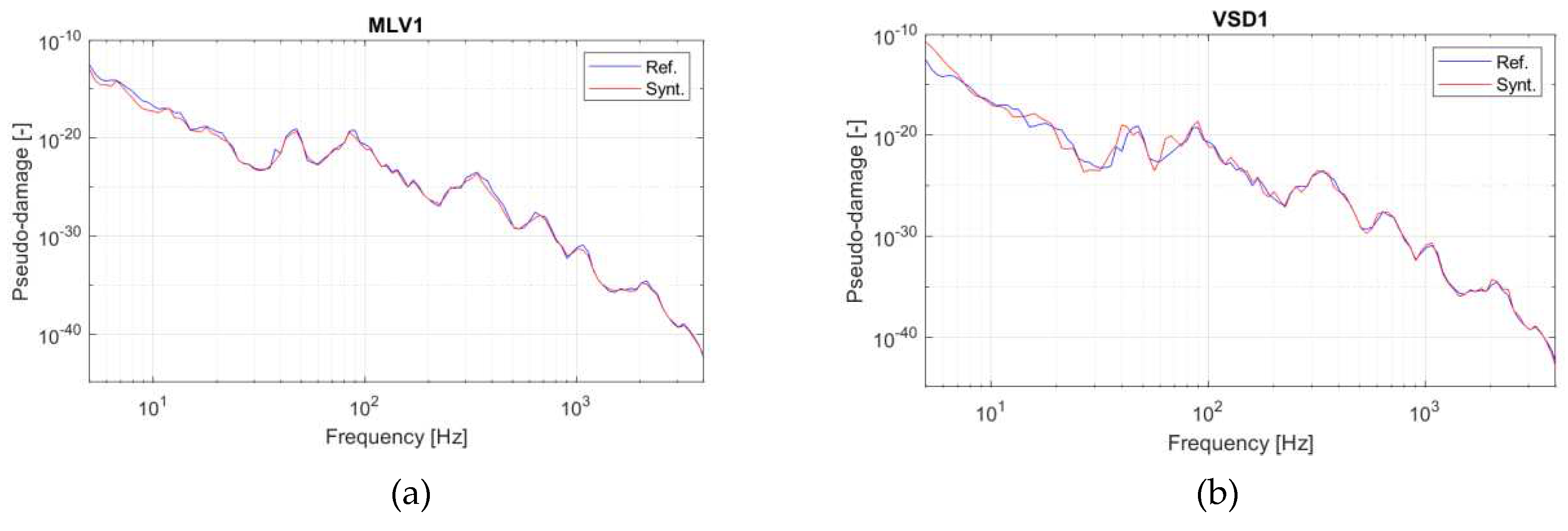
Now, the synthesized and the reference profiles have the same
FDS. It must be highlighted that the newly obtained signals are different from those synthesized previously and their statistical parameters and
PSD change to some extent (
Figure 9 and
Figure 10,
Table 3). However, their nature remains Leptokurtic and similar to the signals MLV1 and VSD1. The plots of the signals
FDSs obtained after convolution with the filter are reported in
Figure 11 and show a precise matching. It is worth noting that the signals in
Figure 9 have a sampling frequency of 10240Hz since an up-sampling was necessary to correctly compute the
FDS, as highlighted in [22, 23]. Though, the
PSDs in
Figure 10 are plotted in the range 0÷4096Hz, consistently with
Figure 1b,
Figure 3,
Figure 6.
4. Discussion
The results show that the MLV algorithm synthesizes shaker input signals that can transfer their kurtosis value to the output of any SDOF linear system, irrespective of the latter’s natural frequency. This aspect eliminates the main flaw of Phase Manipulation and Polynomial Transformation methods. In particular, the kurtosis of the output features small fluctuations around a value close to the excitation one, due to the following reason: all the blocks constituting the synthesized signal have a wideband PSD, thus resonance effects cannot occur. The kurtosis transfer is only due to the energy of the bursts appearing in the signal, and the high excursions in the output cannot physically contain more energy. However, the input parameters of the algorithm are relevant and may affect the results. In fact, if the bursts duration (represented by parameter Tb) is not long enough, the system may not have time to respond and high excursions may not appear in the response. In addition, the MLV algorithm only deterministically imposes the phases of one block, thus achieving a high randomness. Consequently, different runs of the algorithm – with unchanged setup parameters – to process the same reference signal provide the synthesis of different time-series (all complying with the target PSD and kurtosis). Therefore, random vibration tests that require a sizable duration can be carried out starting from short environmental measurements by concatenating many profiles synthesized by the MLV algorithm.
The VSD algorithm can generate narrowband blocks, which can exasperate resonance effects on the DUT: the lower the value of parameter p, the more evident the resonance occurrence. The advantages of this algorithm are two-fold: (i) the synthesized signals are capable of generating SDOF systems responses with high kurtosis, though the excitation features relatively small value of the crest factor, thus subjecting the shaker to non-critical loads; (ii) kurtosis of the response is not constant over the natural frequency and is generally broadly higher than the excitation one (this scenario being quite common in many practical applications, due to the variable spectrogram of real-life vibrations). It must be highlighted, however, that a significant limitation of the algorithm could be that the PSD variation cannot be controlled. On the other side, its randomness contributes to the synthesized signal stochasticity, which is further increased by the complete aleatory generation of the phases in the IFFT transform for each block.
Both the algorithms could lead to signals with a very different damage potential from the excitation one, since kurtosis control does not directly control the
FDS. The filter described in [
20] was used to correct the
FDSs of the signals generated by both the
MLV and the
VSD algorithms. The new signals showed similar Leptokurtic distributions as their corresponding synthesized ones, with slightly different
PSD and statistical parameters. The procedure was used to synthesize signals having the same duration as that of the reference input, for the sake of direct comparison of results, but is actually intended to be used for accelerated fatigue-life testing.
5. Conclusions
In this work, two novel kurtosis control algorithms were proposed. The first algorithm, named Multi-Level Variance (MLV), splits the signal to be synthesized into blocks of the same duration and featuring variable variance. Namely, the shape of the PSD of each single block remains the same but scaled by an appropriate factor. The overall PSD and kurtosis approach closely to the reference input ones within a certain tolerance. The Papoulis’ Rule proves not to apply if the parameter that controls the duration of the bursts in the synthesized signal is appropriately chosen. In particular, the kurtosis of the output features the tendency to be constant over the natural frequency range of the DUT.
The second algorithm, named Variable Spectral Density (VSD), splits the signal into blocks of the same duration, not only with variable variance but in general with variable PSD. The overall PSD and kurtosis approach closely to the reference input ones, within a certain tolerance. The Papoulis’ Rule proves to not apply for every value of the only algorithm parameter that depends on the user’s choice. The kurtosis of the output tends to vary conspicuously over the natural frequency range of the DUT, with broadly higher values than those determined by the reference field data.
The damage potential associated with the shaker input signals synthesized by both algorithms proves different from that of the reference field data. The difference in the FDSs functions can be corrected by applying a special filter found in the literature. This leads to the generation of new profiles that match the reference FDS still featuring PSD and kurtosis values very similar to those of the signals synthesized by the algorithms. Hence, the overall procedure can be effectively employed to generate shaker input signals for accelerated fatigue-life testing.
The proposed algorithms have been validated through the application to many case studies, not reported in this paper for the sake of brevity (but a few examples can be partially considered in references [24, 25], where the formulation of the algorithms was not still optimized), starting from different reference field data featuring different characteristics – e.g. kurtosis value, bandwidth, spectral content, duration – thus proving their robustness for different scenarios.
Author Contributions
Conceptualization, EP and MT.; methodology, EP; software, EP; validation, EP and MT; formal analysis, MT and AR; investigation, EP; resources, AR; data curation, EP and MT; writing—original draft preparation, EP and MT; writing—review and editing, MT and AR; visualization, EP and MT; supervision, MT; project administration, AR; funding acquisition, AR. All authors have read and agreed to the published version of the manuscript.
Acknowledgments
This activity was performed in collaboration with Easting S.r.l.s. (Trieste, Italy), that is gratefully acknowledged for cooperation and financial support.
Conflicts of Interest
The authors declare no conflict of interest.
Appendix A
This paragraph focuses on operative aspects associated with the implementation of PM-based methods to control the kurtosis of synthesized signals. A number of kurtosis-control algorithms (in particular the works by Steinwolf, e.g. [5, 8], considered by the Authors as the most significant ones in this field) exploit analytical methods that preserve the
PSD of the reference field data by changing only the phases while keeping constant the amplitudes. Indeed, from Eq. A1 (which is a simpler expression of the equation used by Steinwolf in [
8] to demonstrate the proof of the proposed method) and Eq. A2, it is evident that the kurtosis
k depends on both the signal amplitudes and phases, whereas the
PSD depends on amplitudes only:
It is worth noting that PM procedures based on the direct implementation of Eq. A1 (or equivalent formulations) are not particularly efficient due to the high number of calculations required. From the computational cost standpoint, the procedure based on the following steps is suggested as a simple and efficient implementation of PM methods:
Step 0) starting from the PSD of the reference signal, generate phases randomly;
Step 1) select one of the phases randomly;
Step 2) randomly set another value for that phase between 0 and 2π;
Step 3) perform IFFT and calculate the new kurtosis value via Eq. (5);
Step 4) if the new kurtosis value is closer to the target value, keep the value of the phase changed at step 2, otherwise discard it and restore the former value for that phase;
Step 5) repeat from step 1 until the target is reached.
The upgrade in speed of the method is given by the fact that there is no burdensome analytical formula to compute, and it allows for a very straightforward implementation. However, this procedure may present two major disadvantages if not used along with other methods. The first one regards the filtering of the peaks occurring because of Papoulis’ Rule: in fact, the natural frequency of the DUT should be known a priori, in order to change the phases only in the vicinity of the resonance [
17], otherwise the response may be close to Gaussian [
18]. The second one concerns computational complexity: despite optimizing its implementation, the method is still slower than other commonly used kurtosis-control methods. If PM is implemented, it is suggested to generate a signal by splitting it into blocks in order to create more realistic peaks and decrease computational complexity, since smaller blocks would imply a lower
Nh.
Appendix B
The formulae for kurtosis and variance of a time-series composed of
n signals can be written in the following forms:
where the following nomenclature holds:
n: number of concatenated signals/blocks;
kj: kurtosis of the jth signal/block;
ktot: kurtosis of the overall signal;
σj2: variance of the jth signal/block;
σtot2: variance of the overall signal/block;
Tj: duration of the jth signal/block;
T: duration of the overall signal (

).
These formulae are a generalization of Eqs. (10, 12) because, in that case, the blocks had the same duration. Their proof is given next, with the assumption that a signal
xj has zero mean (without loss of generality). From the definition of the
sth statistical moment
Mstot of the signal
xj:
and the definition of the following parameters:
Ntot: number of samples of the overall signal;
ns: number of samples of the sth signal/block;
Ns: sum of the number of samples of the 1st, 2nd,…, sth signal/block.
Equation (B1) can be derived from the following equalities:
In the last step,
M4s represents the 4
th statistical moment of the
sthblock. By substituting the definition for kurtosis Eq. (B1) is found:
Similarly, Eq. (B2) can be derived in the following way:
By substituting the definition for the second-order moments Eq. (B2) is found:
Appendix C
The procedure reported in
Section 3, which permits to adjust the
FDS based on the filter proposed by Kihm
et al. [
20], is mathematically justified. Let the following quantities be defined:
D(fn): value of the Fatigue Damage if the DUT had a natural frequency equal to fn;
x(t): signal synthesized by any kurtosis control algorithm;
T: duration of x(t);
h(t): impulse response of the system/DUT;
z(t): relative displacement between the SDOF system mass and the base excitation at time t;
Δz: half-cycle belonging to the histogram of z(t);
p(Δz): probability density of Δz;
K: proportionality constant between mechanical stress and relative displacement;
b: exponent of Wohler’s curve;
C: constant in Wohler’s curve;
Np: number of positive peaks per unit time of a signal.
The expected damage caused by the signal
x(
t) can be expressed via the following equation [
2]:
Equation (C1) could be equivalently re-written in terms of
z(
t) in the following way:
where
p(
t1,
t2) is the probability density to find a valley/trough at instant
t1 and its corresponding peak at instant
t2. Since
z(
t) can be related to
x(
t) via convolution:
Eq. (C2) can also be put in the following form:
Let us now assume that the Fatigue Damage Spectrum of
x(
t), namely
E{
D(
fn)}, has been computed and it differs from the reference one, symbolically written as
Dr(
fn). To simplify the mathematical details and arrive at simple results, assume that the spectral function:
can be considered relatively constant over the natural frequency axis. Hence, its Inverse Fourier Transform is approximately proportional to a Dirac delta:
If a new signal

is considered, given by the convolution between
x(
t) and
g(
t) and substituted into Eq. (C4) in place of
x(
t), the following would result:
The steps show that the
FDS of the function

, obtained from convolving
x(
t) with
g(
t), is equal to the reference one. Thus, the filter defined by Eq. (C5) or Eq. (C6) is effective for adjusting the
FDS of a signal synthesized by kurtosis-control methods.
References
- Steinwolf, A. Random vibration testing beyond PSD limitations. Sound & Vibration 2006, 40, 12–21. [Google Scholar]
- Lalanne, C. Mechanical Vibration and Shock Analysis-Volume 5: Specification Development, John Wiley & Sons, Inc-ISTE, London, 2009. S: Vibration and Shock Analysis-Volume 5, 2009.
- Lalanne, C. Mechanical Vibration and Shock Analysis-Volume 3: Random Vibration, John Wiley & Sons, Inc-ISTE, London, 2009. R: Vibration and Shock Analysis-Volume 3, 2009. [Google Scholar]
- Giacomin, J. , Steinwolf, A., Staszewski, W.J. Application of mildly nonstationary mission synthesis (MNMS) to automotive road data. Engineering Integrity 2000, 7, 44–56. [Google Scholar]
- Steinwolf, A. Approximation and simulation of probability distributions with a variable kurtosis value. Computational Statistics and Data Analysis 1996, 21, 163–180. [Google Scholar] [CrossRef]
- Steinwolf, A. , Connon, W.H. Limitations on the use of Fourier Transform Approach to Describe Test Course Profiles. Sound &Vibration 2005, 39, 12–17. [Google Scholar]
- Steinwolf, A. Two methods for random shaker testing with low kurtosis. Sound & Vibration 2008, 42, 18–22. [Google Scholar]
- Steinwolf, A. Vibration testing of vehicle components by random excitations with increased kurtosis. Int. J. Vehicle Noise and Vibration 2015, 11, 39–66. [Google Scholar] [CrossRef]
- Steinwolf, A., Peeters, B., Van der Auweraer, H. Two methods of generating random excitations with increased kurtosis for in-house testing of vehicle components. Proceedings of The 22nd International Congress on Sound and Vibration, Florence, Italy, 2015. 2015.
- Minderhoud, J. , Van Baren, P. Using Kurtosion® to Accelerate Structural Life Testing, Sound & Vibration 2010, 44, 8–12. [Google Scholar]
- Kihm, F. , Ferguson, N.S., Antoni, J. Fatigue life from kurtosis controlled excitations. Procedia Engineering 2015, 133, 698–713. [Google Scholar] [CrossRef]
- Zhang, J., Cornelis, B., Peeters, B., Janssens, K., Guillaume, P. A new practical and intuitive method for kurtosis control in random vibration testing, Proceedings of ISMA, Leuven, Belgium, 2016. 2016.
- Winterstein, S.R. Nonlinear vibration models for extremes and fatigue, ASCE Journal of Engineering Mechanics 1988, 114, 1772–1790. 1988.
- Merritt, R.G. A stochastic model for the pulse method - Part 2: random part. In Annual technical meeting-institute of environmental sciences. Institute of Environmental Sciences, 1997, Vol. 43; pp121–129.
- Smallwood, D.O. Generating non-Gaussian vibration for testing purposes, Sound & Vibrations 2005, 39, 18–24.
- Hsueh, K.D. , Hamernik, R. P. A generalized approach to random noise synthesis: theory and computer simulation, Journal of the Acoustical Society of America 1990, 87, 1207–1217. [Google Scholar]
- Cornelis, B. , Steinwolf, A., Troncossi, M., Rivola, A. Shaker testing simulation of non-Gaussian random excitations with the fatigue damage spectrum as a criterion of mission signal synthesis. Proceedings of the 2015 International Conference on Engineering, Ljubljana, Slovenia, 2015, pp 763–772.
- Papoulis, A. Narrow-Band systems and Gaussianity, IEEE Trans. on Information Theory 1972, 18, 20–27. [Google Scholar] [CrossRef]
- Papoulis, A., Unnikrishna Pillai, S. Probability, Random Variables, and Stochastic Processes, 3rd ed. McGraw-Hill, New York, NY (USA), 1991. 1991.
- Kihm, F., Halfpenny, A., Munson, K. Synthesis of Accelerated and More Realistic Vibration Endurance Tests Using Kurtosis, SAE Technical Paper 2016, 2016-01-0275.
- Lalanne, C. Mechanical Vibration and Shock Analysis-Volume 4: Fatigue Damage, John Wiley & Sons, Inc-ISTE, London, 2009.
- Ahlin, K. Shock Response Spectrum Calculation – An Improvement of the Smallwood Algorithm. Proceedings of the 70th Shock and Vibration Symposium, Albuquerque, NM, 1999.
- McNeill, S.I. Implementing the Fatigue Damage Spectrum and Fatigue Damage Equivalent Vibration Testing. Proceedings of the 79th Shock and Vibration Symposium, Orlando, FL, 2008, Vol. 23.
- Pesaresi, E., Troncossi, M. Synthesis of Vibration Signals with Prescribed Power Spectral Density and Kurtosis Value. Proceedings of the 28th International Conference on Noise and Vibration Engineering - ISMA2018, Leuven (Belgium), 2018, pp. 29–40.
- Troncossi, M. , Pesaresi E. Analysis of synthesized non-Gaussian excitations for vibration-based fatigue life testing, J. Phys.: Conf. Ser. 2019, 1264, 012039. [Google Scholar]
|
Disclaimer/Publisher’s Note: The statements, opinions and data contained in all publications are solely those of the individual author(s) and contributor(s) and not of MDPI and/or the editor(s). MDPI and/or the editor(s) disclaim responsibility for any injury to people or property resulting from any ideas, methods, instructions or products referred to in the content. |
© 2023 by the authors. Licensee MDPI, Basel, Switzerland. This article is an open access article distributed under the terms and conditions of the Creative Commons Attribution (CC BY) license (http://creativecommons.org/licenses/by/4.0/).




 ;
;


 ).
).


 is considered, given by the convolution between x(t) and g(t) and substituted into Eq. (C4) in place of x(t), the following would result:
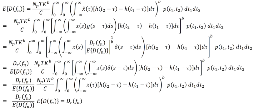
 , obtained from convolving x(t) with g(t), is equal to the reference one. Thus, the filter defined by Eq. (C5) or Eq. (C6) is effective for adjusting the FDS of a signal synthesized by kurtosis-control methods.

