Submitted:
13 September 2023
Posted:
14 September 2023
You are already at the latest version
Abstract
Keywords:
1. Introduction
- Sequence : 10101010101010101010101010
- Secuence : 01101011100110111001011010
- A process generated by some physical or natural process, e.g. radiation, resistor or semiconductor noise (the practitioner’s view).
- A process that cannot be described in a “few words” or succinctly (the instance or descriptional complexity view) - the smaller the description of a sequence of bits can be made, the less random it is (try to apply this to the two sequences above).
- A process that cannot be guessed in a “reasonable” amount of time (the computational complexity view).
- A process that is fundamentally impossible to guess (the “philosophical” view).
- A process possessing certain statistical characteristic of the ideally uniform process (the statistician’s view).
2. Physical Sources of Randomness

3. Pseudorandom Number Generation
- Easy to evaluate:The value is efficiently computable given s and x.
- Pseudorandom:The function cannot be efficiently distinguished from a uniformly random function , given access to pairs , where the ’s can be adaptively chosen by the distinguisher.
- The bits are easy to calculate (for example in polynomial time in some suitable definition of the size parameter, e.g. size of a modulus).
- The bits are unpredictable in the sense that it is computationally intractable to predict in sequence with probability better than , i.e for any computationally feasible next-bit predictor algorithm ,for .
3.1. The Linear Congruential Generator
- The parameter c should be relatively prime to m.
- If m is a multiple of 4 then should, also, be a multiple of 4.
- For all prime divisors p of m the value of should be a multiple of p.
- m is prime,
- a is a primitive element modulo m,
- is relatively prime to m.
3.2. Cryptographically Secure Generators
3.2.1. The BBS Generator
- Find primes p and q such that mod 4
- Set
- Start with = seed (a truly random value),
- Set mod N
- Output the least significant bit of
- Set , go to step 3
3.2.2. The RSA/Rabin Generator
- Find primes p and q as well as a small prime e such that
- Set
- Start with = seed (a truly random value),
- Set mod N
- Output the least significant bit of
- Set and repeat from Step 3
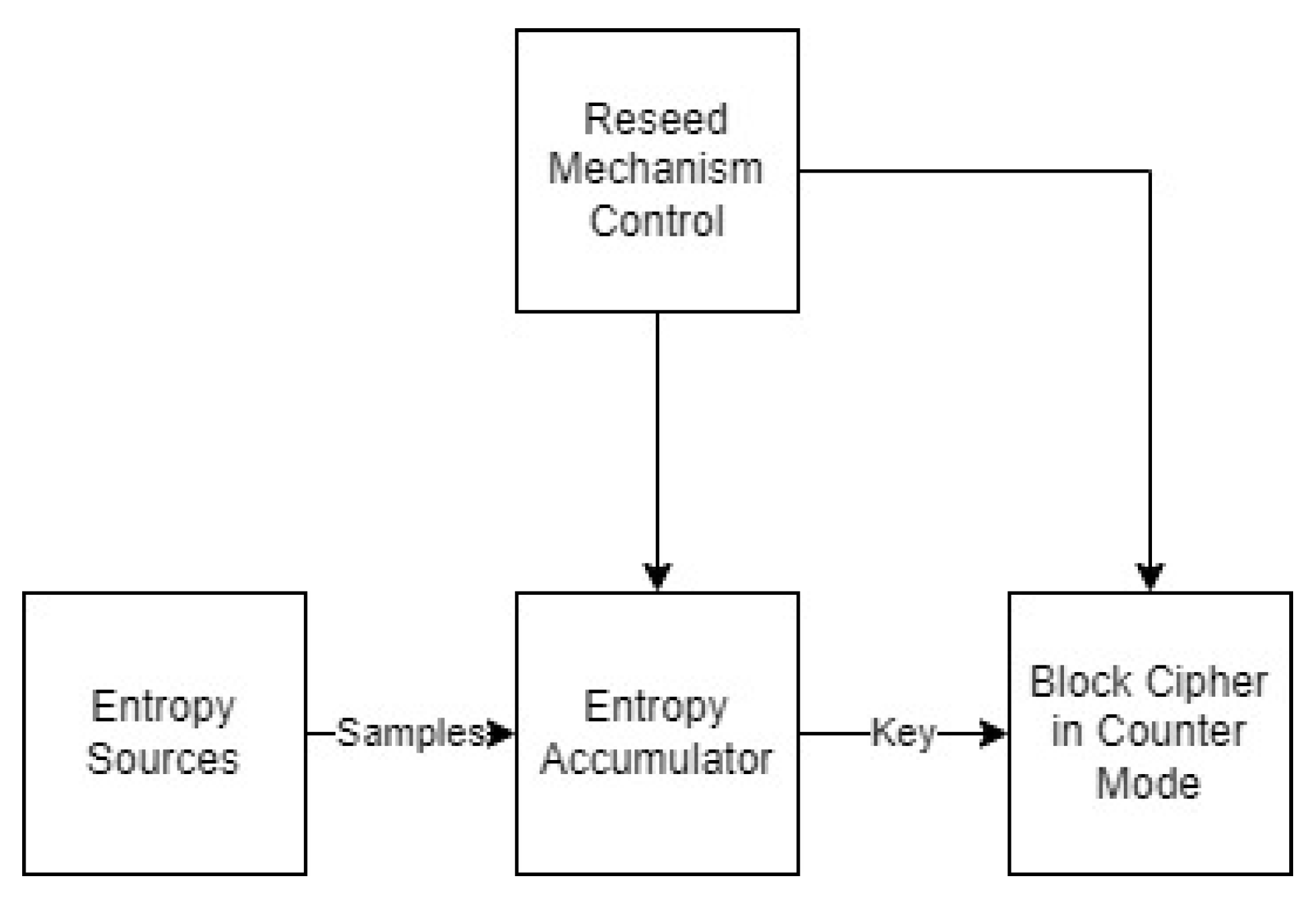
3.2.3. Generators Based on Block-Ciphers
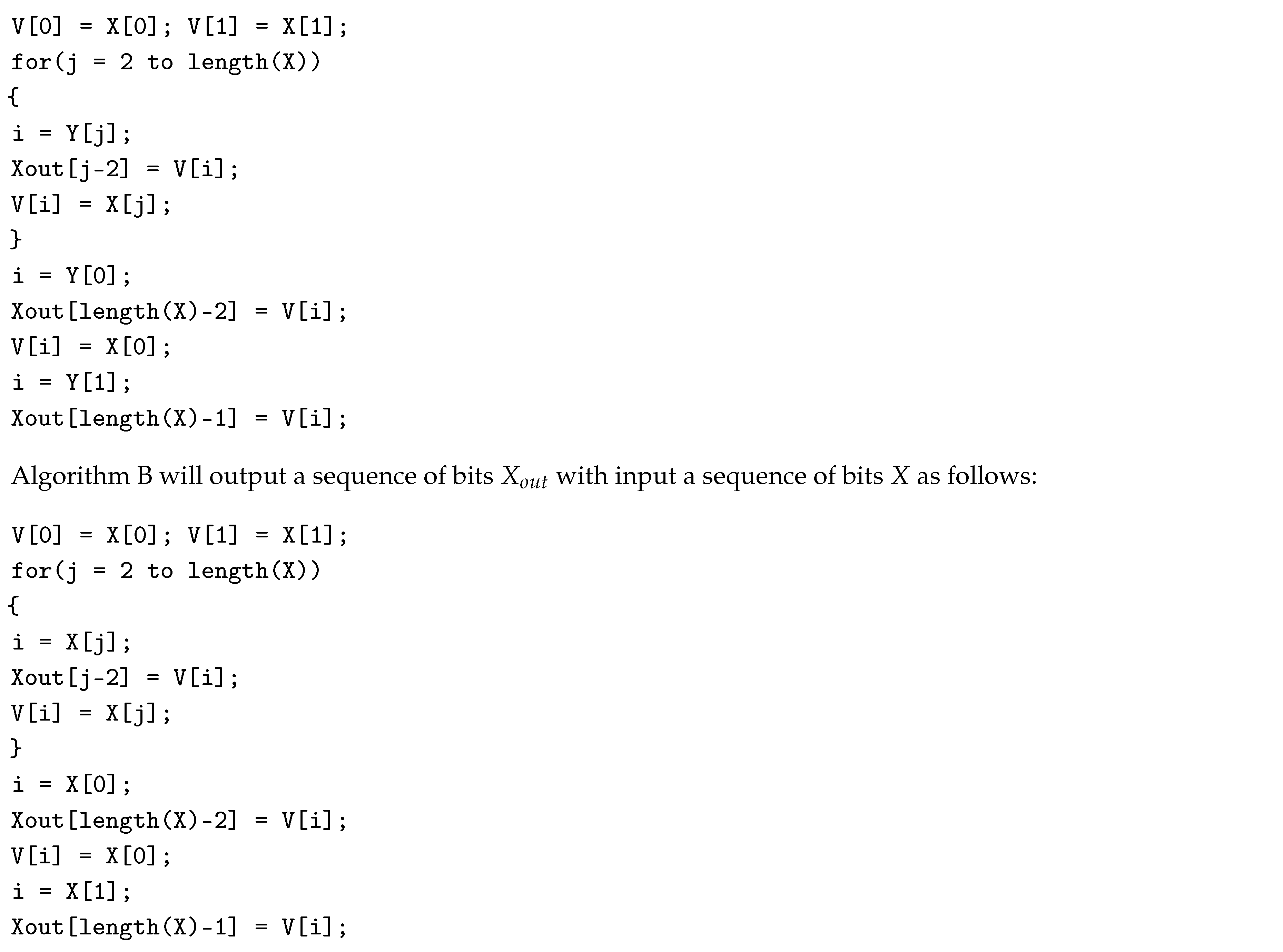
3.2.4. Algorithms M and B

- , where m is the modulus of the sequence X.
- is the next new element of the sequence ,
- We set and is set to the next element of the sequence X.
4. Randomness Tests
4.1. Practical Statistical Tests
4.1.1. The “Chi-Square” Test
- Each observation can belong to one of k categories.
- We have obtained n independent measurements.
4.1.2. The Kolmogorov-Smirnov Test
- First, we take n independent observations corresponding to a certain continuous distribution function .
- We rearrange the observations so that they occur in non-descending order .
- The desired statistical quantities are given by the following formulas:
4.1.3. Equidistribution or Frequency (Monobit) Test
- Using the “Kolmogorov-Smirnov” test with distribution function , for .
- For each element a, , we count the number of occurrences of a in the given sequence and then we apply the “chi-square” test with degree of freedom , and probability for each element (“bin”).
4.1.4. Serial Test
- We count the number of times that pairs occur, for , .
- We apply the “Chi-Square” test with degrees of freedom and probability for each category (i.e. pair).
- The value of n should be, at least, .
- The test can also be applied to groups of triples, quadruples, etc. of consecutive generator values.
- The value of d must be limited in order to avoid the formation of many categories.
4.1.5. Gap Test

4.1.6. Poker Test
- All 5 elements are distinct.
- There is only one pair of equal elements.
- There are two distinct pairs of equal elements each.
- There is only one triple of equal elements.
- There is a triple of equal elements and a pair of equal elements, different from the element in the triple.
- There is one one quadruple of equal elements.
- There is a quintuple of equal elements.
4.1.7. Coupon Collector’s Test
-
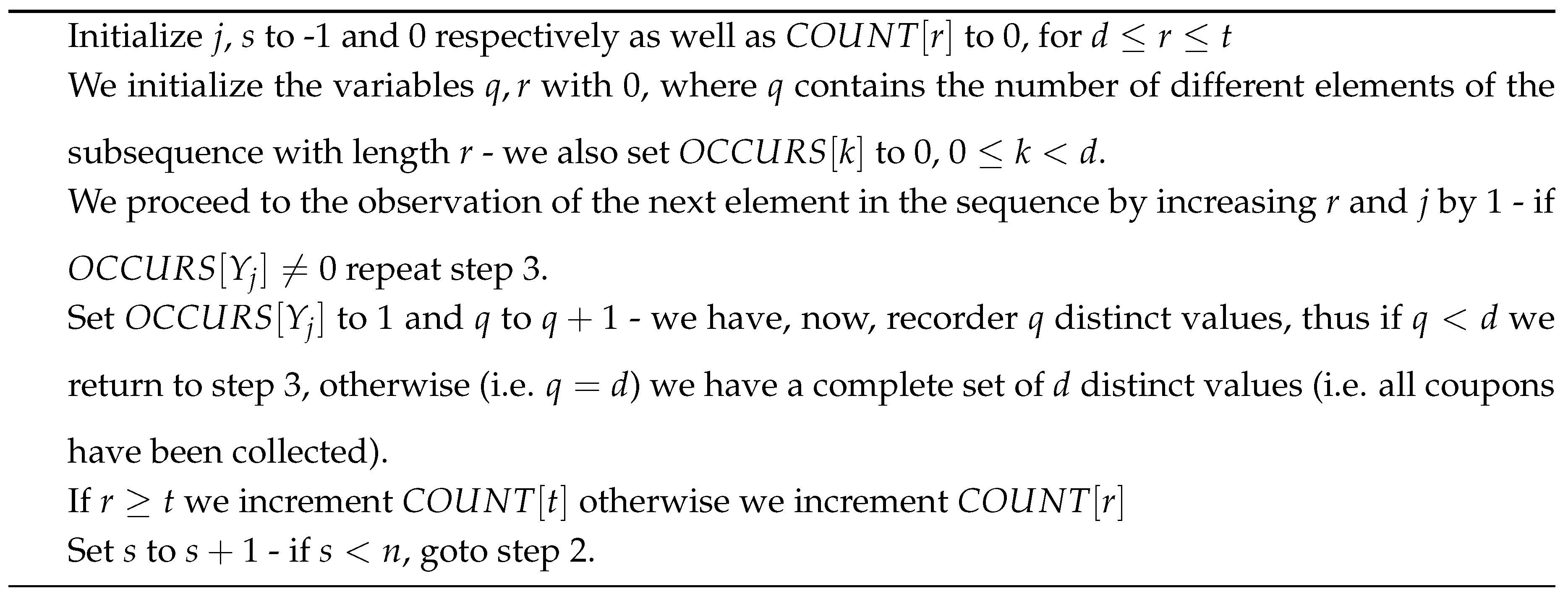
Given the PRNG sequence , where , we count the lengths of n consecutive “coupon collector” samplings using the algorithm that follows. In the algorithm, is the number of segments of length r, , while is the number of segments of length at least t.Algorithm description:
-
After the algorithm has counted n lengths, we apply the “Chi-Square” test to(i.e. the number of coupon collection steps of length r) with (degrees of freedom). The propabilities that correspond to these events are the following (see [12] for the derivation):
4.1.8. Permutation Test

4.1.9. Run Test
- We use an algorithm that measures the lengths of the monotone runs (this is easy to accomplish).
-
After the lengths have been computed, we calculate the statistical indicator V as follows:The values and are specific constants, which are given in [12] in matrix form. The value of V is expected to obey the “Chi-Square” distribution with six degrees of freedom and sufficiently large n, e.g. .
4.1.10. The Maximum t Test
- We take the maximum value of the given t numbers, i.e. for all n subsequences, , .
- We apply the “Kolmogorov-Smirnov” test to the sequence of maximums with distribution function , . As an alternative, we can apply the Equidistribution test to the sequence .
4.1.11. Collision Test
4.1.12. Birthday Spacings Test
4.1.13. Serial Correlation Test
4.2. The Diehard Suite of Statistical Tests
- Birthday spacings: We select random points on a large interval. The spacings between the selected points should be, asymptotically, exponentially distributed (test connected with the Birthday Paradox in probability theory).
- Overlapping permutations: We analyze sequences of five consecutive numbers from the given sequence. The 120 possible orderings are expected to occur with, approximately, equal probabilities.
- Ranks of matrices: We choose a certain number of bits from the numbers in the given sequence and form a matrix over the elements . We then determine the rank of the matrix and compare with the expected rank of a fully random 0-1 matrix.
- Monkey tests: We view the given numbers as “words” in a language. We count the overlapping words in the sequence of the numbers. The number of such “words;; that do not appear should follow the expected distribution (test based on the Infinite Monkey Theorem in probability theory).
- Count the 1’s: We count the 1’s in either successive or chosen numbers from the given sequence. We then convert the counts to “letters” and count the occurrence of 5-letter such “words”.
- Parking lot test: We randomly place unit radius circles in a 100×100 square area. We say that such a circle is successfully parked if it does not overlap with another already successfully parked circle. After 12000 such parking trials, the number of successfully parked circles should follow an expected normal distribution.
- Minimum distance test: We randomly place 8000 points in a 10000×10000 square area. We, then, calculate the minimum distance between all the point pairs. It is expectet that the square of this distance should follow the exponential distributed for a specific mean value.
- Random spheres test: We randomly select 4000 points in a cube of edge 1000. We, then, center a sphere on each of these points, where the sphere radius is the minimum distance to the other points. It is expected the the minimum sphere volume should follow the exponential distribution for a specific mean value.
- The squeeze test: We multiply 231 by random floating numbers in the range until we obtain as a result 1. We repeat this experiment 100000 times. The number of floating points required to obtain 1 should follow an expected distribution.
- Overlapping sums test: We produce a sufficiently long sequence of random floating points in the range . We add the sequence formed by 100 successive floating point numbers. It is expected that these sums follow the normal distribution with a specific variance and mean values.
- Runs test: We generate a sufficiently long sequence of random floating points in the range . We count ascending and descending runs. These counts should follow an expected, from random values, distribution.
- The craps test: We play 200000 games of “craps”, counting the winning games and the number of dice throws for each of these games. These counts should follow an expected distribution.
5. Application Domains Where Unpredictability Is Essential
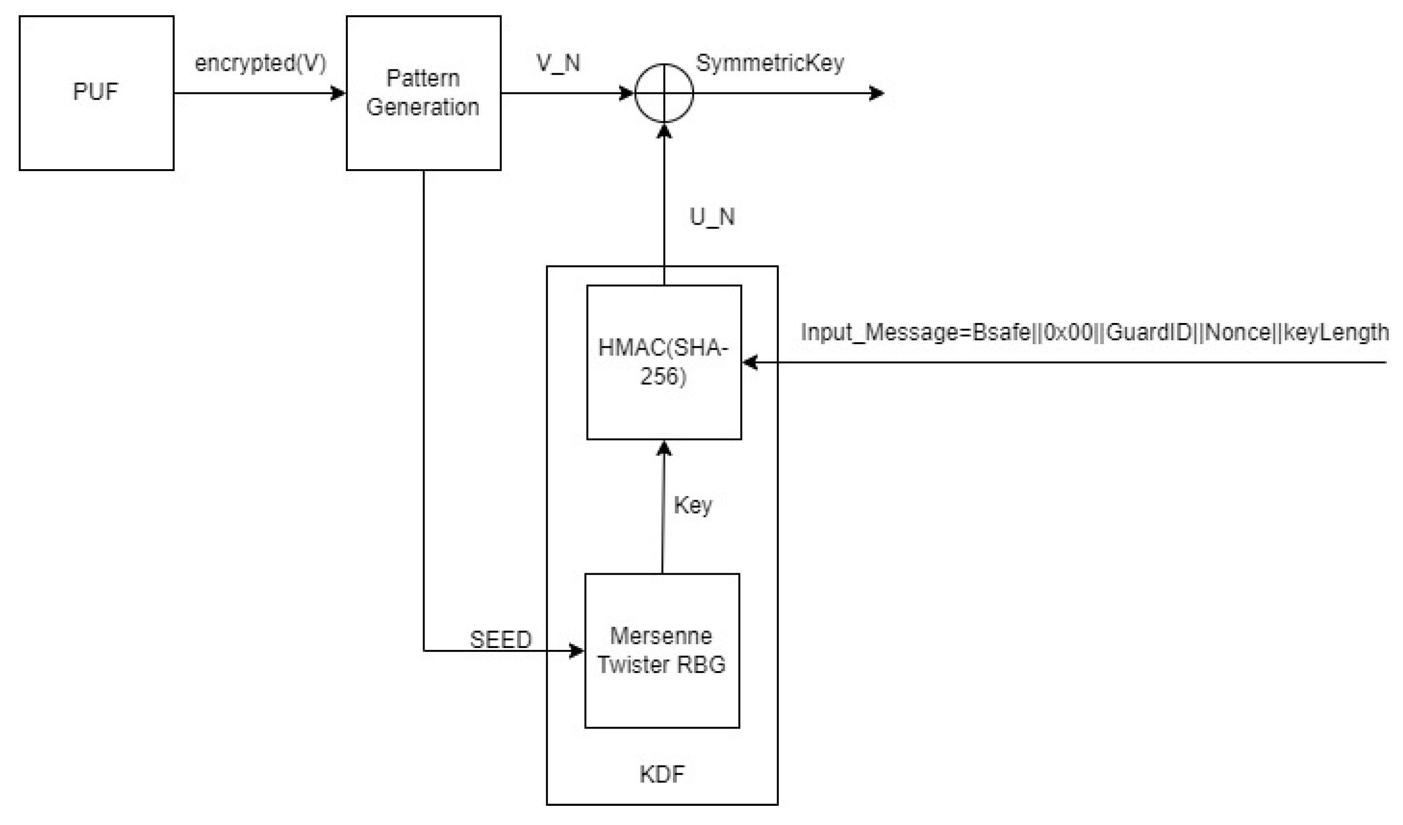
5.1. Cryptographic Key Generation
5.2. Online Electronic Lotteries
- The produced numbers should obey the uniform distribution over the required number range.
- It should be infeasible for anyone (even the lottery owner and operator) to predict the numbers of the next draw, given the draw history, with a prediction probability “better” than the uniform over the range of the lottery numbers.
- It should be infeasible for anyone (even the lottery owner and operator) to interfere with the draw mechanism in any way.
- The draw mechanism should be designed so as to obey a number of standards and, in addition, there should also be a process through which it can be officially certified (by a lottery designated body) that these standards are met by the lottery operator.
- The draw mechanism should be under constant monitoring (by a lottery designated body) so as to detect and rectify possible deviations from the requirements.
- The details of the operation of the lottery draw mechanism should be publicly available for inspection in order to build trust and interest towards the lottery. In addition, this publicity facilitates auditing (which may be required by a country’s regulation about electronic lotteries).
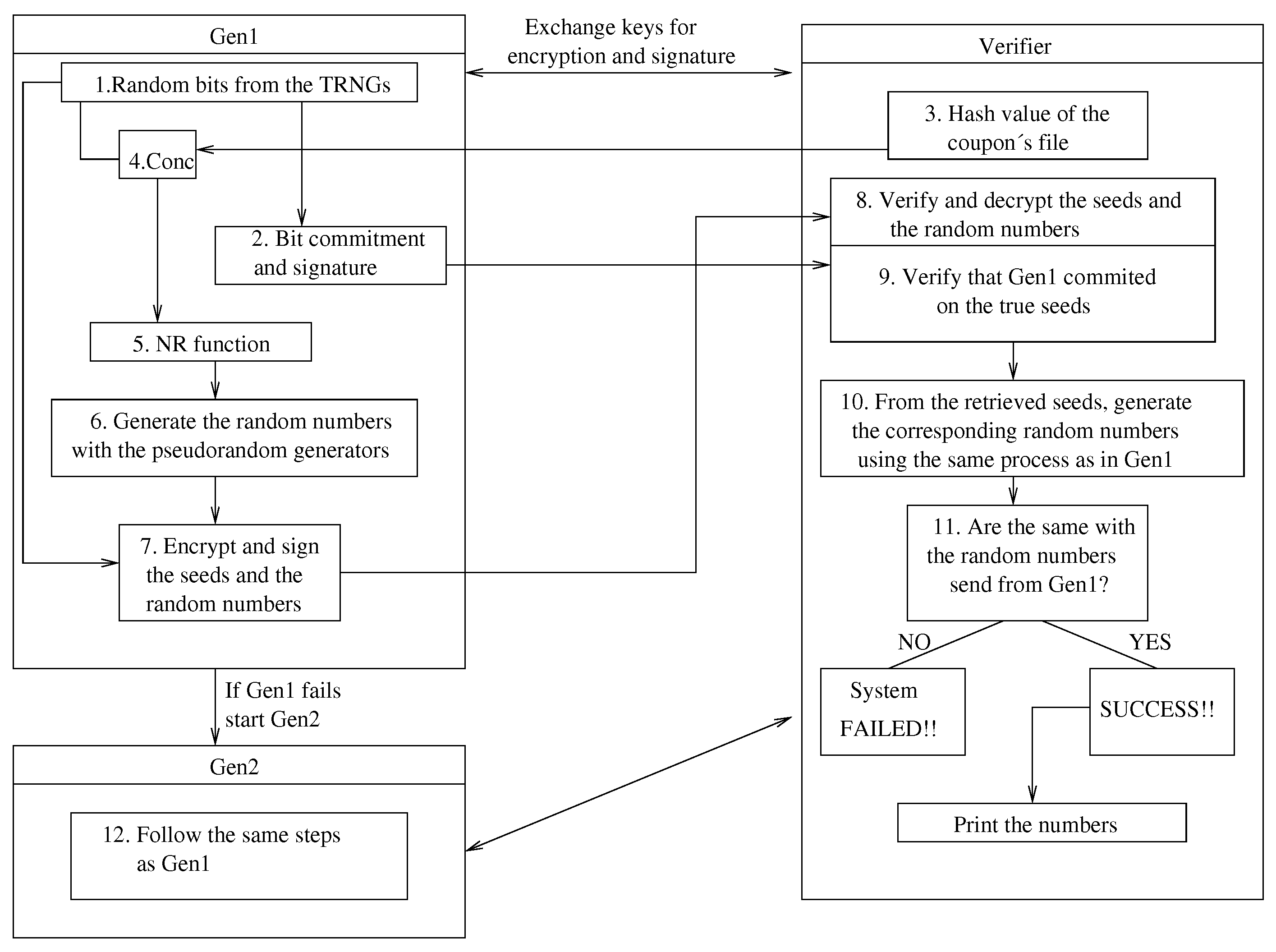
5.3. The Protocol Components
5.3.1. Prevention of Post-Betting
5.3.2. Signing the Numbers and Authenticating Their Source
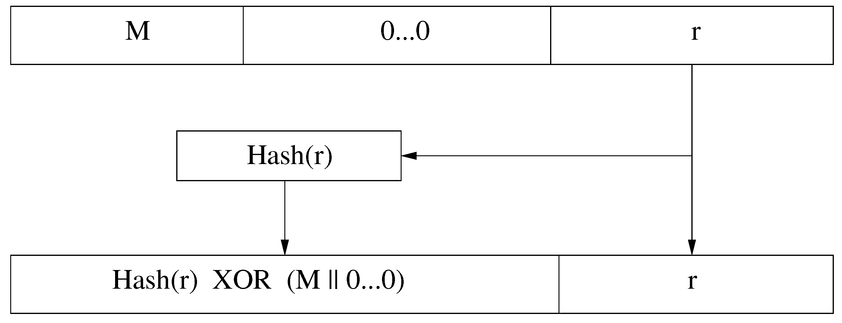
5.3.3. Seed Commitment and Reproduction of Received Numbers
5.3.4. Incorporation of Several True Randomness Sources
5.3.5. Mixing the Outputs of the Generators: Algorithms M and B
5.3.6. Capability for Dynamic, On-Line, Reconfiguration
6. Conclusions
Acknowledgments
References
- Alexi, W.; Chor, B.; Goldreich, O.; Schnorr, C. RSA and Rabin Functions: Certain Parts are as Hard as the Whole. SIAM J. Computing 1988, 17, 194–209. [Google Scholar] [CrossRef]
- E. Barker, A. Roginsky, R. Davis, Recommendation for Cryptographic Key Generation, NIST Special Publication 800-133 Revision 2. 2. [CrossRef]
- Blum, L.; Blum, M.; Shub, M. A Simple Unpredictable Pseudo-Random Generator. SIAM J. Computing 1986, 15. [Google Scholar] [CrossRef]
- Blum, M.; Micali, S. How to Generate Cryptographically Strong Sequences of Pseudo-Random Bits. SIAM J. Computing 1984, 13, 850–864. [Google Scholar] [CrossRef]
- D. Boneh. In Proc. Crypto 2001, pp. 275–291. Lecture Notes in Computer Science, Vol. 2139, Springer-Verlag.
- Boyar, J. Inferring sequences produced by pseudo-random number generators. J. Assoc. Comput. Mach. 1989, 36, 129–141. [Google Scholar] [CrossRef]
- Boyar, J. Inferring sequences produced by a linear congruential generator missing low-order bits. Journal of Cryptology 1989, 1, 177–184. [Google Scholar] [CrossRef]
- Carmichael, R.D. On composite numbers P which satisfy the Fermat congruence aP-1≡1modP. Am. Math. Monthly 1919, 26, 137–146. [Google Scholar]
- Goldreich, O.; Goldwasser, S.; Micali, S. How to construct random functions (extended abstract). Proc. FOCS 1984, 464–479. [Google Scholar]
- J. Guajardo, S. S. Kumar, G. J. Schrijen, P. Tuyls: FPGA Intrinsic PUFs and Their Use for IP Protection. CHES 2007: 63-80.
- G Marsaglia. The Marsaglia Random Number CDROM including the Diehard Battery of Tests of Randomness. Florida State University. 1995. Archived from the original on 2016-01-25. Available online: https://web.archive.org/web/20160125103112/http://stat.fsu.edu/pub/diehard/.
- D. Knuth. The Art of Computer Programming: Volume 2, Seminumerical Algorithms. Addison-Wesley Professional, 3rd edition, 1997.
- O.O. Koçak, F. Sulak, A. Doğanaksoy, and M. Uğuz. Modifications of Knuth Randomness Tests for Integer and Binary Sequences. Commun. Fac. Sci. Univ. Ank. Ser. A1 Math. Stat., Volume 67, Number 2, pp. 64–81, 2018. Available online: https://hdl.handle.net/11511/44973.
- E. Konstantinou, V. Liagkou, P. Spirakis, YC. Stamatiou, and M. Yung. Electronic National Lotteries. In Proc. Financial Cryptography: 8th International Conference, FC 2004, pp. 147–163. Lecture Notes in Computer Science, vol 3110. Springer, Berlin, Heidelberg.
- E. Konstantinou, V. Liagkou, P. Spirakis, YC. Stamatiou, and M. Yung. “Trust Engineering:” From Requirements to System Design and Maintenance - A Working National Lottery System Experience. In Proc. Information Security, ISC 2005, pp. 44–58. Lecture Notes in Computer Science, vol 3650. Springer, Berlin, Heidelberg.
- E. Kranakis. Primality and Cryptography. Wiley-Teubner Series in Computer Science, 1986.
- Mcrypt cryptographic library. Available online: ftp://mcrypt.hellug.gr/pub/crypto/mcrypt.
- J. Kelsey, B. Schneier, and N. Ferguson, Yarrow-160: Notes on the Design and Analysis of the Yarrow Cryptographic Pseudorandom Number Generator, Sixth Annual Workshop on Selected Areas in Cryptography, Springer Verlag, August 1999.
- S. Micali, M. Rabin and S. Vadhan, Verifiable Random Functions. In Proc. 40th Annual Symposium on the Foundations of Computer Science (FOCS `99), pp. 120–130. New York: IEEE Computer Society Press.
- M. Naor and O. Reingold, Number-theoretic constructions of efficient pseudo-random functions, Proc. 38th IEEE Symp. on Foundations of Computer Science, 1997.
- C.W. O’Donnell, G.E. Suh, and S. Devadas, PUF-Based Random Number Generation, MIT CSAIL CSG Technical Memo 481.
- I. Shparlinski. On the linear complexity of the power generator. Kluwer Academic Publishers, Designs, Codes and Cryptography, 23, 5-10, 2001.
- M.S. Turan, E. Barker, J. Kelsey, K.A. McKay, M.L. Baish, M. Boyle, Recommendation for the Entropy Sources Used for Random Bit Generation, NIST Special Publication 800-90B. [CrossRef]
- A. Yao. Theory and Applications of Trapdoor Functions. IEEE FOCS, 1982.
- H. Zenil (ed.). Randomness through computation. Collective Volume. World Scientific, 2011.
Disclaimer/Publisher’s Note: The statements, opinions and data contained in all publications are solely those of the individual author(s) and contributor(s) and not of MDPI and/or the editor(s). MDPI and/or the editor(s) disclaim responsibility for any injury to people or property resulting from any ideas, methods, instructions or products referred to in the content. |
© 2023 by the authors. Licensee MDPI, Basel, Switzerland. This article is an open access article distributed under the terms and conditions of the Creative Commons Attribution (CC BY) license (http://creativecommons.org/licenses/by/4.0/).


