Directional Graph Attention Networks

Preprint

Article

Directional Graph Attention Networks

Altmetrics

Downloads

133

Views

Comments

Jiaqi Zhu^*

This version is not peer-reviewed

Submitted:

12 September 2023

Posted:

14 September 2023

You are already at the latest version

Alerts

Abstract

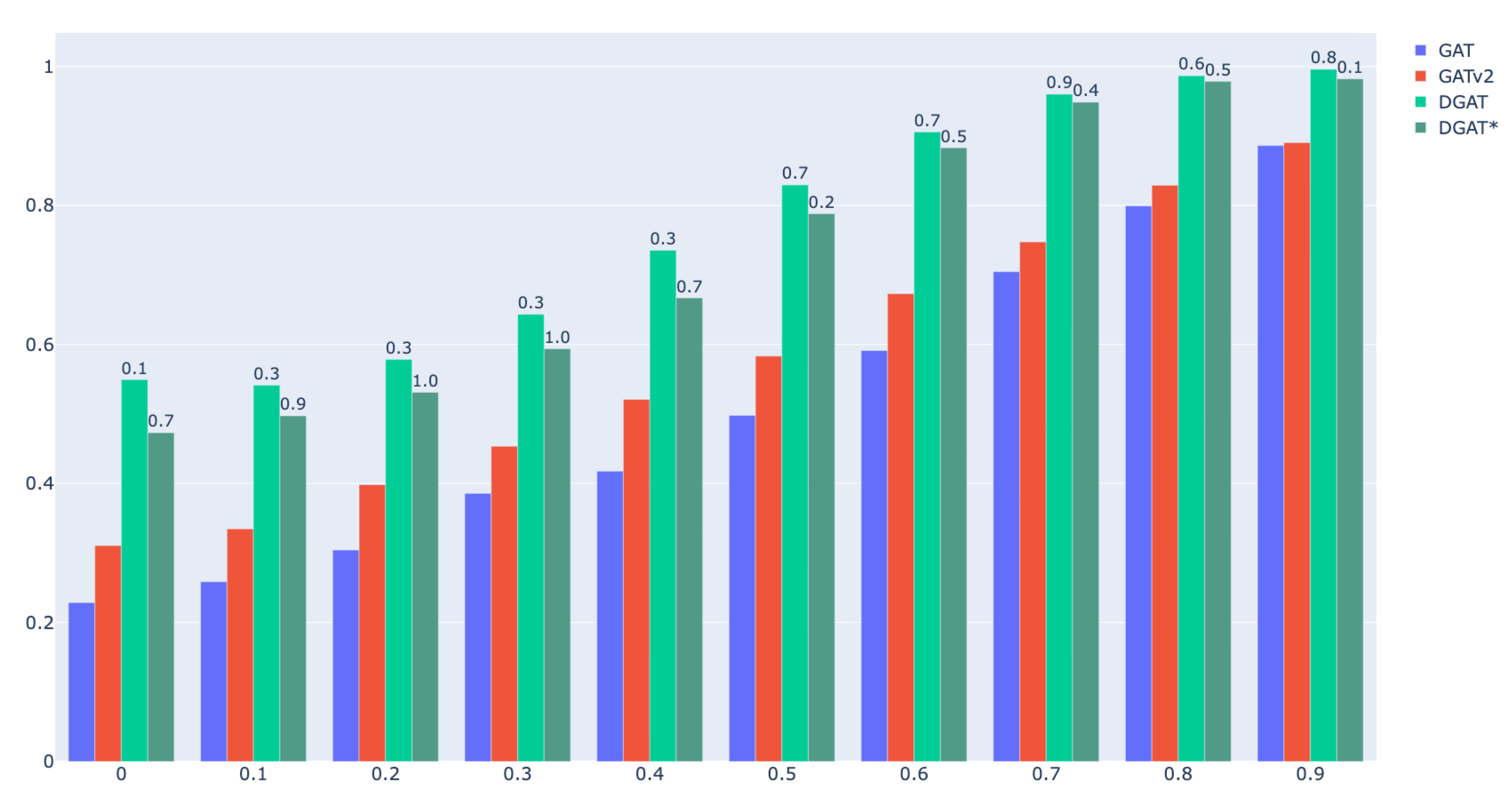
In recent years, graph neural networks (GNNs) have become a promising method for analyzing data structured in graph format. By considering connections between entities in a graph, GNNs are able to extract valuable insights. One notable variation of GNN is the graph attention network (GAT), which employs the attention mechanism and has demonstrated promising performance in various applications. However, its ability to incorporate feature information from nodes beyond the immediate neighborhood is limited, leading to degraded performance on heterophilic data. To address this limitation, this thesis proposes a novel attention-based model, namely the Directional Graph Attention Network (DGAT). This model combines the feature-based attention with the global directional information extracted from the graph topology, as inspired by the Directional Graph Network (DGN). A new class of Laplacian matrices is proposed and an existing theoretical result on DGN is extended. This extension bridges a gap in the literature. The experimental results presented in the thesis, based on nine real-world benchmarks and ten synthetic data sets, demonstrate the superiority of the proposed DGAT model compared to the GAT baseline model. Particularly on heterophilic data sets, DGAT showed a notable average increase of approximately 35% in node classification tasks across all heterophilic real-world data sets. In addition, DGAT outperforms GAT by an average margin of around 51% in all ten synthetic data sets with various levels of heterophily

Keywords:

Subject: Computer Science and Mathematics - Artificial Intelligence and Machine Learning

1. Introduction

The field of deep learning has gained much attention in recent years. People have achieved state-of-the-art results on many distinct tasks in fields such as natural language processing and computer vision by utilizing neural network models.

In those fields where deep learning methods proved to be effective, the data fed into the models are all structured and Euclidean (e.g. 1-dimensional sequence text/audio data and 2-dimensional grid image data). Nevertheless, there also exist an extensive amount of real-world data that cannot be represented using those regular data structures. Those data have more complex underlying structures and can be found in many domains like biology, chemistry, social network analysis and e-commerce, to name a few. Naturally, graphs are chosen to be the best data structure for representing them.

The inherent complexity and irregularity of graph data have imposed significant challenges on existing deep learning models. When working with graph structured data, the traditional deep learning models often discard the connectivity between the data entities and ignore the topological structure of it, which often lead to potential information loss and poor performance results. Over the years, new models have been proposed to address those issues. This new generation of deep learning models built directly to work with graph-structured data is often referred to as graph neural networks (GNNs).

Graph neural networks learn the representation of the input graph by generating embeddings of each graph node in a lower-dimensional space. The embedding generation of a node is done recursively by aggregating information of its neighbours. This mechanism of embedding generation is also referred to as the message passing framework. Depending on the downstream tasks, the node-level embedding can also be used to obtain a graph or subgraph level representation.

LeCun et al. are the pioneer in the filed of graph deep learning, they combined graph signal processing and convolutional neural networks [1]; since then, various GNN architectures have been proposed [2,3,4,5,6,7,8]. The graph attention network (GAT) [4] has demonstrated promising results in node classification tasks on graphs and stands out among various graph neural network variations. The graph attention mechanism employed by GAT contributes to its success. Additionally, Beaini et al. introduced a novel approach that involves defining and leveraging a vector field on the graph. This integration of global topological information enhances the GNN architecture with remarkable effectiveness.

1.1. Goals, Organization and Contributions

The graph attention mechanism adopted by the GAT model is purely based on the local node features, which could lead to performance loss when applied to highly heterophilous graphs [9,10,11]. In this thesis, we aim to mitigate this problem by incorporating topological-based global attention to the original graph attention mechanism. In particular, we introduce a brand-new attention-based model, the DGAT model. By utilizing two mechanisms, namely the neighbour pruning and global directional aggregation, the DGAT model is able to enhance the graph attention mechanism and outperform the GAT model by a large margin on all real-world heterophilic node classification benchmarks in the experiment. Furthermore, in the synthetic experiments we conducted, the DGAT model also demonstrates strong performance and outperformed both the GAT and the GATv2 model by large margins on all datasets with different homophily level.

In Chapter 2, we provide the background knowledge required to understand the rest of the thesis, including a brief introduction to graph representation learning and the essential concepts in general neural networks as well as in graph neural networks.

The review of related work to this thesis is given in Chapter 3. The topics covered in this chapter include graph convolution networks, graph attention mechanism, and how to define and utilize direction in a general graph.

In Chapter 4, we propose the so-called Directional Graph Attention Network (DGAT) based on the directional aggregation mechanism proposed by Beaini et al. [7]. The design principle and the vectorized implementation of the model are explained thoroughly in the chapter. In addition, the training and inference processes are also outlined Chapter 4.

In Chapter 5, we explain the details of our experiment settings, as well as the datasets we used in the experimental study. In addition, we also present and analyze the experiment results in this chapter. We demonstrate the effectiveness of the DGAT model, especially for the highly heterophilous graphs, by comparing its performance with the original Graph Attention Network (GAT) on nine different real-world datasets, as well as ten distinct synthetic datasets. Additionally, we conducted a performance comparison between the DGAT model and the Directional Graph Network (DGN) proposed by Beaini et al., which likewise employs the directional aggregation mechanism. This comparison was carried out on the same nine diverse real-world datasets.

Finally, the summarization of this thesis and discussion regarding further research directions are presented in Chapter 6.

1.2. Notation

In this section, we introduce some notation and terms to be used in this thesis.

We use

G : = (V, E)

to denote a graph with the vertex set

V

and the edge set

E

. Unless specifically mentioned, all graphs G are undirected.

We denote scalars by normal type letters (usually lowercase letters, occasionally upper case letters), column vectors by boldface lowercase letters and matrices by boldface upper case letters.

We use

R

and

Z

to denote the sets of real scalars and integer scalars respectively, and

R^{n}

and

Z^{n}

to denote the set of n-dimensional real vectors and integer vectors, respectively; moreover,

R^{m \times n}

and

Z^{m \times n}

are used to denote

m \times n

real matrices and integer matrices, respectively.

For a column vector

x \in R^{n}

x_{i : j}

denotes the subvector composed of elements of

x

with indices from i to j,

x_{i}

x (i)

denotes the i-th element of

x

For a matrix

A \in R^{m \times n}

A_{i : j, k : l}

denotes the submatrix containing all the elements of

A

whose row indices are from i to j and column indices are from k to l,

A_{i, :}

denotes the

i^{t h}

row of

A

, and

A_{:, j}

denotes the

j^{t h}

column of

A

. The

(i, j)

element of

A

is denoted by

a_{i j}

A (i, j)

. The transpose of matrix

A

is denoted by

A^{T}

We also define some special vectors and matrices here. We use

1_{n}

to denote the n-vector of ones and

0_{n}

to denote the n-vector of zeros (sometimes the subscript n may be omitted). We use I to denote an identity matrix and

e_{k}

to denote the k-th column of the identity matrix I.

We use

A | | B

[\begin{matrix} A \\ B \end{matrix}]

to denote column concatenation of matrix

A

and

B

, and

[A, B]

to denote the row concatenation of matrix

A

and

B

. We use ⊙ to represent element-wise matrix product operator.

For a set S,

| S |

denote the number of elements S has. For a function f of

x

\nabla_{x} f

denotes the gradient of function f with respect to

x

2. Preliminary

This chapter provides the background knowledge needed to understand the rest of the thesis. It first gives a high level description of the graph representation learning in Section 2.1. Then it introduces basic concepts of neural networks, including the multi-layer perceptron and the back propagation algorithm in Section 2.2. Afrer that it briefly discuses structured neural networks for grids and sequences, namely the convolutional neural network and recurrent neural network, in Section 2.3. Finally, an overview of graph neural network is provided in Section 2.5.

2.1. Graph Representation Learning

A graph is defined as

G : = (V, E)

, where

V = {v_{1}, v_{2}, \dots, v_{n}}

is a finite set of nodes of size n, and

E

is a finite set of edges. An edge

e_{i j}

in the edge set

E

are expressed as a tuple of nodes

(v_{i}, v_{j}) \in V \times V

. The adjacency matrix

A \in R^{n \times n}

of G is defined as follows:

a_{i j} = \{\begin{matrix} 1, & e_{i j} \in E \\ 0, & o t h e r w i s e \end{matrix}

The degree matrix

D \in R^{n \times n}

of G is a diagonal matrix whose i-th diagonal entry

d_{i}

represents the number of direct neighbours

| N (v_{i}) |

a node

v_{i}

has, i.e.,

d_{i} = | N (v_{i}) | = \sum_{v_{j} \in N (v_{i})} a_{i j}

. A graph G may have a node feature matrix

X \in R^{n \times d}

whose

i^{t h}

row is the transpose of the feature vector

x_{i} \in R^{d}

of node

v_{i}

Another important type of matrix related to a graph G is the Laplacian matrix [12]. Typically, three different Laplacian matrices are commonly used in practice, namely the unnormalized (or combinatorial) Laplacian, random-walk (or degree) normalized Laplacian and symmetric normalized Laplacian:

L = D - A, L_{rw} = D^{- 1} L, L_{sym} = D^{- 1} L D^{- 1}

(2.1)

The eigenvalues and eigenvectors of Laplacians are important in graph representation learning. Since

L

is symmetric and positive semi-definite, it has n non-negative eigenvalues. Often the eigenvalues are arranged in the ascending order. Note that it is easy to see

L 1 = 0

. Thus the smallest eigenvalue of

L

is 0 and is its one corresponding eigenvector.

The random walk Laplacian matrix

L_{rw}

and the symmetric normalized Laplacian matrix

L_{sym}

shares the same set of eigenvalues, which are between 0 and 2. For the same eigenvalue, the corresponding eigenvectors

ϕ_{rw}

L_{rw}

and

ϕ_{sym}

L_{sym}

have the simple relation:

ϕ_{rw} = D_{ϕ sym}^{\frac{1}{2}}

Graph representation learning aims to learn low-dimensional representations that encode structural information about the graph (so-called embeddings) at different levels, including the node level, sub-graph level and graph level [13]. The learned embeddings of the graph can be further used for different downstream machine tasks, such as node classification, link prediction, community detection and clustering.

Traditionally, graph representations are generated based on graph statistics, kernel functions or hand-engineered features. However, those approaches are limited due to their inflexibility and difficulty of generalizing [14].

Recently, there has been a surge of graph neural network-based graph embedding methods and has drawn much research attention. The key idea of those approaches is to encode nodes into vectors by compressing their local neighbourhood information [15,16]. More details about this class of methods will be presented in later sections.

2.2. Neural Network Basics

2.2.1. Neural networks

Neural networks are computation models inspired by human brains. They are modelled by early descriptions of neuron activity, characterized by a linear operation followed by a typically nonlinear activation function [17]. The artificial neurons (as shown in Figure 1) are the building block of neural networks. Each neuron performs some simple computations, and those interconnected units form neural networks.

The right image of Figure 1 shows a detailed structure of an artificial neuron (also called perceptron), where

x_{1}, x_{2}, \dots, x_{n}

are numerical value input units taken from the raw input or output of other perceptrons, and

x_{0} = 1

, which is introduced for the sake of writing convenience (see later);

w_{1}, w_{2}, \dots, w_{n}

are weight parameters that control the level of importance of each input, and

w_{0}

is a bias parameter, usually written as b. The optimal values for

w_{i}

for

i = 0, 1, \dots, n

are obtained during the learning process of the neural network.

As shown in Figure 1, a perception first takes the inputs

x_{1}, x_{2}, \dots, x_{n}

, multiplies them by weights,

w_{1}, w_{2}, \dots, w_{n}

, and add the bias term b, which can be written

w_{0} \cdot x_{0} = b \cdot 1

. Then, it computes the weighted sum:

z = \sum_{i = 0}^{n} w_{i} \cdot x_{i}

(2.2)

Finally, a nonlinear activation function

f (\cdot)

is applied to get the output y. We can write the output y as:

y = f (\sum_{i = 0}^{n} w_{i} \cdot x_{i})

(2.3)

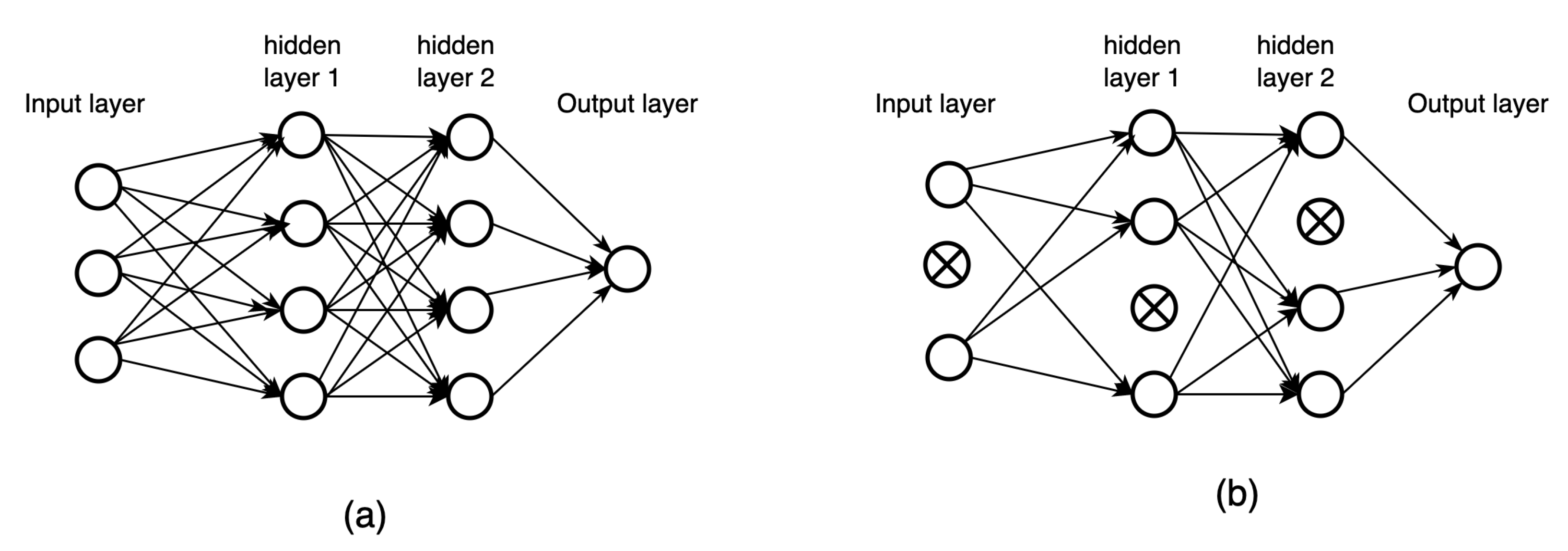
Multi-layer perceptron (MLP) is the most basic neural network, where the neurons are organized into layers. MLP has an input layer, one or more hidden layers and an output layer. The input layer takes input values and passes them to the hidden layer, which processes the input data and presents it to the output layer. Each layer consists of several neurons, and each neuron is fully interconnected to neurons in the subsequent layer; furthermore, a weight is associated with each connection. A neuron computes the weighted sum of outputs from the previous layer and applies a non-linear activation function to it.

As mentioned earlier, an MLP is layered; thus, it is helpful (and commonly what people do in practice) to represent a single-layer unit in the matrix form. Moreover, people often take a step further and express the entire MLP in the matrix form. Notation-wise, it is a common practice to only use

x

to denote the input vector at the input layer, and use

h

to represent the input vector to other layers. We will adopt this convention in this thesis.

Let

h^{(k - 1)} \in R^{d_{k - 1} + 1}

represents the input vector to layer k (where

d_{k - 1}

is the dimension of input with an additional bias term):

\begin{matrix} h^{(k - 1)} = {[1, h_{1}^{(k - 1)}, h_{2}^{(k - 1)}, \dots, h_{d_{k - 1}}^{(k - 1)}]}^{T} \end{matrix}

where we let

h^{(0)} = x

Let

W^{(k)} \in R^{(d_{k} + 1) \times (d_{k - 1} + 1)}

represents the weight matrix at the

k^{t h}

layer of an MLP:

\begin{matrix} W^{(k)} & = [\begin{matrix} w_{00}^{(k)} & w_{01}^{(k)} & \dots & w_{0 d_{k - 1}}^{(k)} \\ w_{10}^{(k)} & w_{11}^{(k)} & \dots & w_{1 d_{k - 1}}^{(k)} \\ \dots & \dots & \dots & \dots \\ w_{d_{k} 0}^{(k)} & w_{d_{k} 1}^{(k)} & \dots & w_{d_{k} d_{k - 1}}^{(k)} \end{matrix}] \end{matrix}

where

d_{k}

is the size of that layer. The matrix-vector product

W^{(k)} h^{(k - 1)} \in R^{d_{k} + 1}

contains all the linear combinations in the

k^{t h}

hidden layer of the MLP, where the

i^{t h}

entry can be expressed in a fashion similar to (2.2):

{(W^{(k)} h^{(k - 1)})}_{i} = w_{i 0}^{(k)} + \sum_{j = 1}^{n} w_{i j}^{(k)} h_{j}^{(k - 1)}

Next, we can extend the notation of activation function

f (\cdot)

to deal with the general matrix as input. For a matrix

A \in R^{m \times n}

, we define

f (A) = [\begin{matrix} f (a_{11}) & f (a_{12}) & \dots & f (a_{1 n}) \\ f (a_{21}) & f (a_{22}) & \dots & f (a_{2 n}) \\ \dots & \dots & \dots & \dots \\ f (a_{m 1}) & f (a_{m 2}) & \dots & f (a_{m n}) \end{matrix}]

i.e., f is an element wise function.

Finally, with this notion we developed, the matrix representation of (2.3) at the

k^{t h}

layer can be written as:

h^{(k)} = f^{(k)} (W^{(k)} h^{(k - 1)})

(2.4)

where

k \geq 1

. In particular, the

i^{t h}

entry of

h^{(k)}

can be written as

h_{i}^{(k)} = {(f^{(k)} (W^{(k)} h^{(k - 1)}))}_{i} = f^{(k)} (w_{i 0}^{(k)} + \sum_{j = 1}^{n} w_{i j}^{(k)} h_{j}^{(k - 1)})

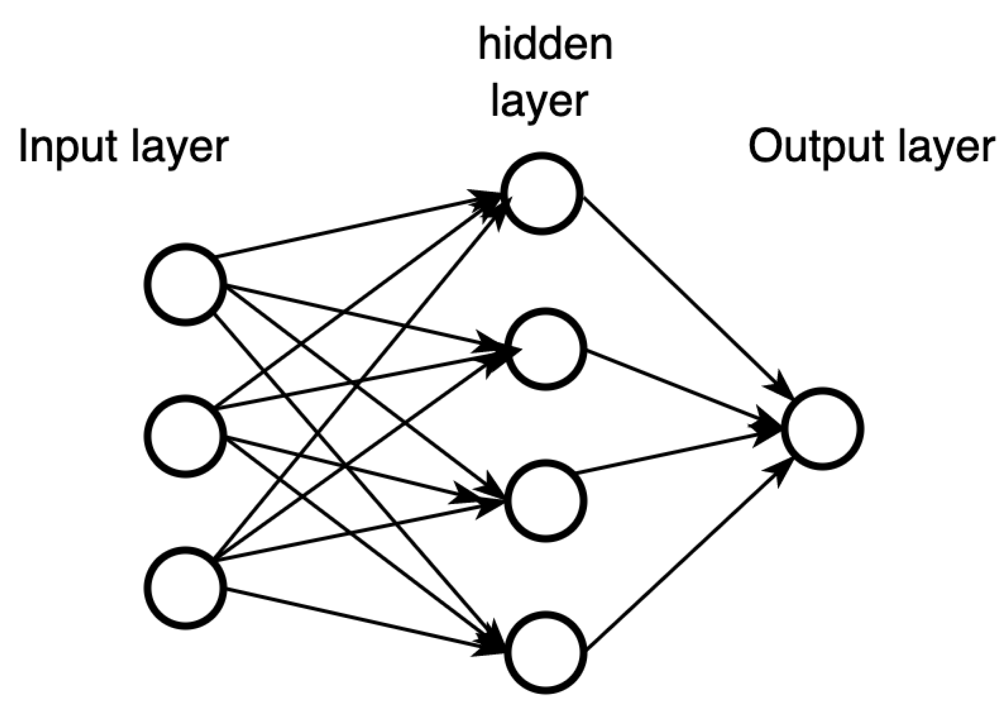
Figure 2 shows an example of MLP with an input of size 3, one hidden layer of size 4, and an output layer of size 1, which can be represent as:

y = f^{(2)} (\sum_{i = 0}^{4} w_{i}^{(2)} \cdot f^{(1)} (\sum_{j = 0}^{3} w_{i j}^{(1)} \cdot x_{j}))

(2.5)

where

x_{j}

denotes the input j,

w_{i j}^{(1)}

denotes the weight from input unit j to hidden unit i in the hidden layer;

w_{i}^{(2)}

denotes the weight from hidden unit i in the hidden layer to output unit in the output layer;

f^{(1)} (\cdot)

and

f^{(2)} (\cdot)

denote the activation function in hidden and output layer respectively; and y denotes the output.

Equation (2.5) can be written in matrix form as:

y = f^{(2)} (W^{(2)} f^{(1)} (W^{(1)} x))

where

x \in R^{4 \times 1}

W^{(1)} \in R^{5 \times 4}

, and

W^{(2)} \in R^{1 \times 5}

There are a few commonly used activation functions.

Hyperbolic tangent ( $t a n h$ ) is defined as $\tanh (z) = \frac{e^{z} - e^{- z}}{e^{z} + e^{- z}}$ . It is non-linear, continuously differentiable, and has a fixed output range (between -1 and 1) [18]. The biggest problem $t a n h$ activation gives rise to is the “vanishing gradients” problem, which causes weights stop updating, this concept will be further explained in the next section.
Rectied Linear Unit function (ReLU) is defined as ReLU $(z) = \max (0, z)$ [19]. It avoids the vanishing-gradient issue and can be evaluated quickly. However, it suffers from the “dead neurons” problem, in which the neurons with $z < 0$ stop outputting anything other than 0.
LeakyReLU is defined as LeakyReLU $(z) = \max (α z, z)$ , where $α$ is a hyperparameter that represents the slope of the function for $z < 0$ (see [20]) It addresses the “dead neurons” problem by making a small variations.
The softmax function is a function that takes an n-dimensional column (resp. row) vector $z$ and outputs an n-dimensional column (resp. row) vector $\tilde{z}$ :

${\tilde{z}}_{i} : = softmax {(z)}_{i} = \frac{\exp (z_{i})}{\sum_{j = 1}^{n} \exp (z_{j})}$

Note that each ${\tilde{z}}_{i} \in (0, 1)$ and $\sum_{i} {\tilde{z}}_{i} = 1$ . Thus, these elements can be interpreted as probabilities.

2.2.2. Back-propagation

Back-propagation [21], an efficient algorithm used for training neural networks, is considered one of the most fundamental building blocks in deep learning.

Each back-propagation step consists of two passes, namely a forward pass and a backward pass. The predicted output is evaluated against the expected result in the forward pass; moreover, all the intermediate results are preserved since they are used later in the backward pass. The algorithm first measures the network’s output error during a backward pass using a cost function; it then computes the error gradient by the chain rule and propagates it through all the hidden layers until it reaches the input layer. Finally, the computed error gradients are used to update the network’s parameters (weights and biases).

Let’s first define the general forward pass of a MLP with K hidden layers. We denote the input layer as the 0^th layer and the output layer the

{(K + 1)}^{t h}

layer. Given the input vector

x

, we define

h^{(0)} = x

. Then for

k \in {1, 2, \dots, K + 1}

, we have:

\begin{matrix} Weighted sum at hidden layer k : & z^{(k)} = W^{(k)} h^{(k - 1)} \\ Activated weighted sum at hidden layer k : & h^{(k)} = f^{(k)} (z^{(k)}) \end{matrix}

Finally, we denote the output of the network

h^{(K + 1)}

y

As mentioned in preceding paragraph, the network’s output error (also called loss) is then measured by using the output vector

y

against an expected output vector

\bar{y}

using a cost function:

C = cost (y, \bar{y})

The expected output

\bar{y}

is part of the training data and is associated with the input

x

, which is often expressed as a tuple

(x, \bar{y})

. Depending on the task, there are different choices of the cost function. Some commonly used ones include MSE (mean squared error) and cross-entropy. The smaller the loss returned by the cost function C, the closer the output

y

is to the expected output

\bar{y}

The objective during the neural network training process is to minimize the loss with respect to the weights for the training data set. The most common method for solving such a problem is the stochastic gradient descent method [22], which solves the minimization problem in an iterative manner. In particular, at each iteration we use the back-propagation algorithm to compute the gradient of the loss with respect to the weights, and then update the weights accordingly. We need to calculate the derivative of C with respect to every weight in the network, starting from the output layer and working backwards through the network to the input layer:

\frac{\partial C}{\partial w_{i j}^{(k)}}

(2.6)

where

k \in {1, \dots, K + 1}

with K being the total number of hidden layers,

w_{i j}^{(k)}

is the weight of unit i in layer

k - 1

to unit j in layer k in the network. With the help of chain rule, this computation can be done efficiently.

Let

W

be the representation of the weight matrices

W^{(k)}

for

k = 1, \dots, K + 1

of the network. In matrix notation, (2.6) can be expressed as:

\nabla_{W^{(k)}} C (W) = (\frac{\partial C (W)}{\partial w_{i j}^{(k)}})

To emphasize C is a function of the variable

W

, here we write C as

C (W)

, but often we omit

W

for simplicity.

In the output layer, the gradient

\nabla_{y} C

is a column vector:

\begin{matrix} \nabla_{y} C & = [\begin{matrix} \frac{\partial C}{\partial y_{1}} \\ \frac{\partial C}{\partial y_{2}} \\ ⋮ \\ \frac{\partial C}{\partial y_{m}} \end{matrix}] \end{matrix}

where m is the number of output units. The gradient of C with respect to the weighted sum

z^{(k)}

at the

k^{t h}

hidden layer (i.e.,

z^{(k)} = W^{(k)} h^{(k - 1)}

\nabla_{z^{(k)}} C

, can be defined in the similar fashion.

Since

y = f^{(K + 1)} (z^{(K + 1)})

, by applying the chain rule, we can compute the gradient of C with respect to the weighted sum vector

z^{(K + 1)}

at the output layer as:

\nabla_{z^{(K + 1)}} C = \nabla_{y} C ⊙ \frac{\partial f^{(K + 1)}}{\partial z^{(K + 1)}}

where ⊙ is the element-wise product operator (so-called Hadamard product) and

\begin{matrix} \frac{\partial f^{(K + 1)}}{\partial z^{(K + 1)}} : = \frac{\partial f^{(K + 1)} (z^{(K + 1)})}{\partial z^{(K + 1)}} & = [\begin{matrix} \frac{\partial f^{(K + 1)} (z_{1}^{(K + 1)})}{\partial z_{1}^{(K + 1)}} \\ \frac{\partial f^{(K + 1)} (z_{2}^{(K + 1)})}{\partial z_{2}^{(K + 1)}} \\ ⋮ \\ \frac{\partial f^{(K + 1)} (z_{m^{'}}^{(K + 1)})}{\partial z_{m^{'}}^{(K + 1)}} \end{matrix}] \end{matrix}

Since

z^{(k + 1)} = W^{(k + 1)} f^{(k)} (z^{(k)}) = W^{(k + 1)} [\begin{matrix} f^{(k)} (z_{1}^{(k)}) \\ ⋮ \\ f^{(k)} (z_{n}^{(k)}) \end{matrix}]

\begin{matrix} \frac{\partial C}{\partial z_{j}^{(k)}} & = \sum_{j} \frac{\partial C}{\partial z_{j}^{(k + 1)}} \frac{\partial z_{j}^{(k + 1)}}{\partial f^{(k)}} \frac{\partial f^{(k)}}{\partial z_{i}^{(k)}} \\ = (\sum_{j} \frac{\partial C}{\partial z_{j}^{(k + 1)}} w_{j i}^{(k + 1)}) \frac{\partial f^{(k)}}{\partial z_{i}^{(k)}} \end{matrix}

Then we have

\nabla_{z^{(k)}} C = ({(W^{(k + 1)})}^{T} \nabla_{z^{(k + 1)}} C) ⊙ \frac{\partial f^{(k)}}{\partial z^{(k)}}

Note that

z^{(k)} = W^{(k)} h^{(k - 1)}

. Thus,

w_{i j}^{(k)}

is involved only in

z_{i}^{(k)}

. Specifically,

z_{i}^{(k)} = \sum_{ℓ} w_{i ℓ}^{(k)} h_{ℓ}^{(k - 1)}

. Therefore,

\frac{\partial z_{i}^{(k)}}{\partial w_{i j}^{(k)}} = h_{j}^{(k - 1)}

Then

\begin{matrix} \frac{\partial C}{\partial w_{i j}^{(k)}} & = \frac{\partial C}{\partial z_{i}^{(k)}} \frac{\partial z_{i}^{(k)}}{\partial w_{i j}^{(k)}} & = \frac{\partial C}{\partial z_{i}^{(k)}} h_{j}^{(k - 1)} \end{matrix}

Write the above equality in matrix-vector form:

\nabla_{W^{(k)}} C = \nabla_{z^{(k)}} C \cdot {(h^{(k - 1)})}^{T}

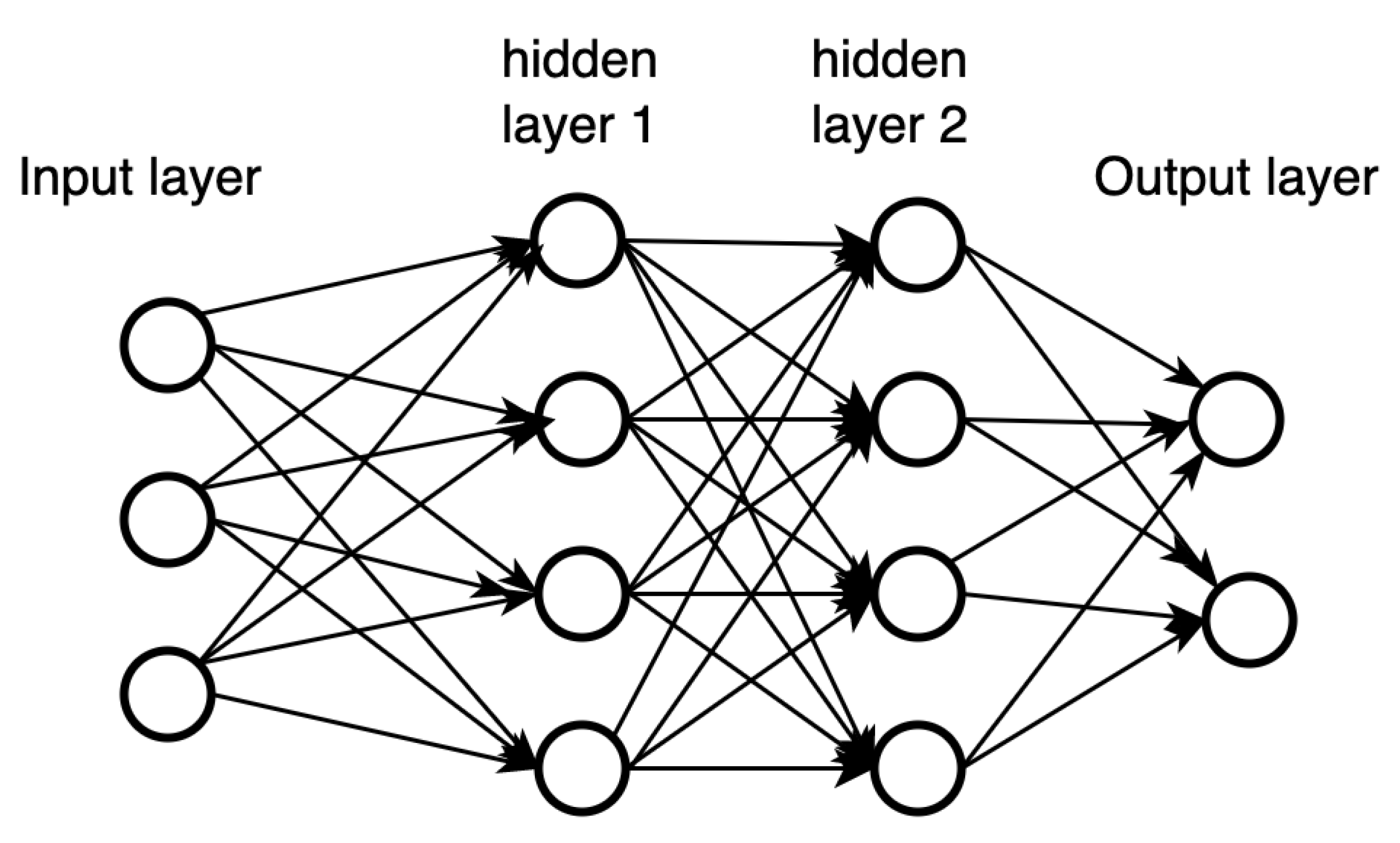
To demonstrate the idea of the back-propagation algorithm, we will use a more complex-structured MLP with two hidden layers and two output units, as shown in Figure 3.

The forward pass of the network can be expresses by the following set of equations :

\begin{matrix} Input layer : & h^{(0)} = x \\ Weighted sum at hidden layer 1 : & z^{(1)} = W^{(1)} h^{(0)} \\ Activated weighted sum at hidden layer 1 : & h^{(1)} = f^{(1)} (z^{(1)}) \\ Weighted sum at hidden layer 2 : & z^{(2)} = W^{(2)} h^{(1)} \\ Activated weighted sum at hidden layer 2 : & h^{(2)} = f^{(2)} (z^{(2)}) \\ Weighted sum at output layer : & z^{(3)} = W^{(3)} h^{(2)} \\ Final output : & y = f^{(3)} (z^{(3)}) \end{matrix}

We first write the cost function of our network as a function of weights by substituting the output

y

by the explicit expression of each layer:

\begin{matrix} C & = (\bar{y}, f^{(3)} (z^{(2)})) \\ = (\bar{y}, f^{(3)} (W^{(3)} h^{(2)})) \\ = (\bar{y}, f^{(3)} (W^{(3)} f^{(2)} (z^{(1)}))) \\ = (\bar{y}, f^{(3)} (W^{(3)} f^{(2)} (W^{(2)} h^{(1)}))) \\ = (\bar{y}, f^{(3)} (W^{(3)} f^{(2)} (W^{(2)} f^{(1)} (z^{(1)})))) \\ = (\bar{y}, f^{(3)} (W^{(3)} f^{(2)} (W^{(2)} f^{(1)} (W^{(1)} h^{(0)})))) \\ = (\bar{y}, f^{(3)} (W^{(3)} f^{(2)} (W^{(2)} f^{(1)} (W^{(1)} x)))) \end{matrix}

Next, we compute the gradient of C with respect to the weight

W^{(3)}

in the output layer as:

\nabla_{W^{(3)}} C = \nabla_{y} C \cdot {(h^{(2)})}^{T}

where

\begin{matrix} \nabla_{y} C & = [\begin{matrix} \frac{\partial C}{\partial y_{1}} \\ \frac{\partial C}{\partial y_{2}} \end{matrix}] \end{matrix}

Then we calculate the gradient of C with respect to the weight

W^{(2)}

in the hidden layer 2:

\nabla_{W^{(2)}} C = \nabla_{z^{(2)}} C \cdot {(h^{(1)})}^{T}

where

\nabla_{z^{(2)}} C = ({(W^{(3)})}^{T} \nabla_{y} C) ⊙ \frac{\partial f}{\partial z^{(2)}}

Lastly, we can calculate the gradient of C with respect to the weight

W^{(1)}

in the hidden layer 1:

\nabla_{W^{(1)}} C = \nabla_{z^{(1)}} C \cdot {(h^{(0)})}^{T}

where

\nabla_{z^{(1)}} C = ({(W^{(2)})}^{T} \nabla_{z^{(2)}} C) ⊙ \frac{\partial f}{\partial z^{(1)}}

As mentioned earlier, the chain rule is the key ingredient in gradient computation. In order to avoid the redundant computations of intermediate terms in the chain rule, the back-propagation algorithm starts backward from the last layer, as in the sample computation we showed above.

Once the gradients are computed, we can update the weights in the k-th layer of the network by:

W^{(k)} : = W^{(k)} - ϵ \cdot \nabla_{W^{(k)}} C

where

ϵ

is a hyperparameter that controls how much the weights are being adjusted with respect to the gradient, and it is often referred to as the learning rate. Weights for each layer is updated in a sequential order.

A common practice people have adopted to ensure a neural network trains properly is to initialize the weights randomly before running it, which is sometimes referred to as "break symmetry" between neurons [23]. If two neurons at the same hidden layer have the same initial weights, then their weights may be updated similarly during the training process and remain indistinguishable from each other at each iteration. In this case, the model may be biased towards a particular set of weights and fail to generalize the input data. Another common pitfall worth mentioning during the initialization stage is that, if initialized weights of a neural network are too small or too large, it may lead to undesired phenomena often referred to as the “vanishing gradient” and “exploding gradient” problem. In particular, “vanishing gradient” describes the scenario where the gradients become smaller and approach zero as the back-propagation algorithm advances backwards from the output layer towards the input layer, which eventually leaves the weights of the lower layers of a neural network nearly unchanged. On the contrary, “exploding gradient’ describes the situation where the gradients become larger and larger as the back-propagation progresses, which causes huge weights update and makes the gradient descent algorithm diverge. Some initialization methods, such as Xavier’s initialization [24] and He’s initialization [25] are often used for network weight initialization, which can significantly alleviate the vanishing/exploding gradient problem.

2.3. Structured Neural Networks for Grids and Sequences

This section will briefly introduce two types of specialized neural networks targeting two distinct input forms: the convolution neural network that processes grid-like data and the recurrent neural network that processes sequential data.

Notice that only the bare minimal information will be provided. The goal is to assist readers in better understanding the later content of this thesis, which is the neural network on the graph.

2.3.1. Convolutional neural networks

Convolutional neural networks (CNNs) are a specialized class of neural networks designed for processing grid-like data. The typical inputs of a CNN are order d tensors, which represents images with h height, w width and d colour channels. Figure 4 shows a typical CNN architecture, which consists of a series of interleaved convolutional and pooling layers (we showed only one convolution and polling layer in the figure). Until the input is reduced sufficiently, it will be fed into and processed by an MLP.

The main building block of CNNs is the convolution layer, which is based on a mathematical operation called convolution. In a convolution layer, a convolution operator slides the parameter tensor along the input tensor and measures the summation of their element-wise multiplication.

Figure 5 demonstrates how a

2 \times 2

convolution operator (kernel) works on an image represented by a

3 \times 4 \times 1

tensor. The sliding of the kernel starts from the top-left corner, and it keeps moving towards the right until it reaches the border of the image. The kernel then returns to the left of the image and moves down by an element. This process is repeated until the kernel reaches the bottom-right of the image. The element-wise product between the kernel and its overlapped area (so-called the receptive field) with the image tensor is computed at each location. The convolution result will then be the summation of the products.

Recall from the preceding section that, in an MLP, each neuron is connected with all the other neurons. However, this is not always the case with CNNs. In a CNN, each neuron in a convolutional layer is only connected to neurons in its receptive field. This particular property of CNNs is often referred to as sparse connectivity. Sparse connectivity enables CNNs to have fewer parameters in a convolution layer; furthermore, it allows the parameters to be used as the kernel moves to different locations (so-called parameter sharing). The parameter sharing encodes a structural bias: a feature extracted by a convolution kernel is important, no matter where it happens in the image. Note that it is conventional to apply a nonlinear layer after a convolutional layer, with the same purpose of the activation function in the MLP, which is to insert non-linearity.

Once one or more convolutional layers are applied to the input image, another critical ingredient of CNNs comes into play, namely the pooling layer. A pooling layer’s primary function is to successively reduce the size of the computed convolution representation, which further reduces the number of parameters and computations in the network. The reduction is made by retaining only the most critical information in a spatial neighbourhood of the input representation. One of the most commonly used pooling layers is max-pooling, which takes a filter and moves over the input patches across each channel and transforms them by taking only the maximal value.

2.4. Recurrent neural networks

Recurrent neural networks (RNNs) are a specialized class of neural networks designed for processing sequential data. The most typical input of RNNs is text data, which consist of arbitrarily many words. One thing to notice is that before feeding the input text into an RNN, people often first convert each word in the text into a feature vector.

Similar to CNNs, RNNs also use a special layer to process the input data, namely the recurrent layer. A recurrent layer is composed of the recurrent neuron. The input of each recurrent layer at time step t consists of two types of data: the new input from time t and the hidden representation generated from time

t - 1

. Just like the inputs, there are also two types of outputs produced by a recurrent layer at each time step t, the hidden representation and the RNN output.

Figure 6 shows an example of the typical RNN architecture.

Since there are two types of inputs for each recurrent neuron, there will also be two sets of weights associated with each input type; and just like CNNs, those weights are shared and updated across time steps.

More specifically, as illustrated in Figure 6, for each time step t,

x_{t} \in R^{n}

is the input feature vector,

h_{t} \in R^{p}

is the hidden representation, which can be expressed as:

h_{t} = f_{h} (W_{h x} x_{t} + W_{h h} h_{t - 1})

and

y_{t} \in R^{m}

is the RNN output vector, which can be repressed as:

y_{t} = f_{y} (W_{y} x_{t})

where

W_{h x} \in R^{p \times n}

is the weight matrix associated with the input in the recurrent layer,

W_{h h} \in R^{p \times p}

is the weight matrix associated with the hidden units in the recurrent layer,

W_{y} \in R^{m \times n}

is the weight matrix associated with the hidden units in the to the output;

f_{h} (\cdot)

and

f_{y} (\cdot)

are nonlinear activation functions.

2.5. Graph Neural Networks

Inspired by the success of convolutional neural netroks (CNNs) and recurrent neural networks (RNNs), people attempted to apply neural network models to graphs. Gori et al. were the first who outlined the notion of graph neural networks [26]; later on, the idea was further developed by Scarselli et al. in their work [2] and Gallicchio et al. in the work [27]. Those graph neural network models share a similar spirit as the RNN models (also referred to as RecGNNs), which aims to learn representations for each node via recurrent neural architecture. An important assumption made by this type of GNNs is that a node and its neighbours are constantly exchange information/propagate messages until a stable equilibrium state is reached [28]. Another family of graph neural network models that inherits the idea from CNN architectures was developed in parallel by redefining the convolution for graph data. Bruna et al. developed the first ConvGNNs based on spectral graph theory [29]. A representation of each node is generated iteratively based on its own representation and the representation of its neighbours (referred to as the message passing process). One key distinction between ConvGNNs and RecGNNs is that, ConvGNNs stack several graph convolutional layers to extract high-level node representation. Right after their introduction, ConvGNNs successfully proved their effectiveness, and the idea of message passing became the fundamental building block of constructing graph neural networks.

Formally, we can define the architecture of a graph neural network (GNN) as follows: A GNN typically takes a graph

G : = (V, E)

represented by the adjacency matrix

A

and a node feature matrix

X

as inputs, and it outputs a set of node-level representation vectors

{h_{u} : \forall u \in V}

, or a single graph-level representation vector

h_{G}

2.6. The message-passing framework

As mentioned in the proceeding section, most modern GNNs adopt the message-passing framework, in which the representation

h_{u}

of node u is generated by iteratively aggregating the representation of its neighbours, as well as its own representation generated from the previous layer. The

k^{t h}

layer of a GNN can be represented by the two following operations [14]:

where

m_{u}^{(k)}

is the aggregated message by applying the AGGREGATE operator to node u’s direct neighbours,

N (u)

; and

h_{u}^{(k)}

is the representation vector for node u at the

k^{t h}

layer generated by using the UPDATE operator (in practice, people often initialize

h_{u}^{(0)}

to be the feature vector

x_{u}

), and

N (u)

is the set of neighboring nodes of u. Since the AGGREGATE function operates on a subset of nodes, it should be invariant under the permutation; some commonly used AGGREGATE functions are: mean, sum and max function.

The operators AGGREGATE and UPDATE in a GNN model have learnable parameters similar to other types of neural networks (refer to Chapter 3 for more details), and the choice of the operators varies in different models, but most of GNNs can be expressed by the above two expressions [14].

2.7. Different types of graph learning tasks

Typically, GNNs are used for three levels of downstream tasks, namely the node level task, edge level task and graph level task.

In a node-level task, each node

u \in V

is associated with a label (for node classification task) or a target value

y_{u}

(for node regression task), the goal is to learn a representation vector

h_{u}

of u so that the label or target value associated with u can be accurately predicted using such representation.

Edge-level tasks are sometimes referred to as relation prediction or link prediction tasks. Typically, an incomplete set of edges

\tilde{E}

between the nodes is given in such a task. The goal is to learn a representation vector for each node, such that given node representations

h_{u}

and

h_{v}

of node u and v, where

u v \in E

and

u v \notin \tilde{E}

, the missing edge

u v

can be accurately inferred by utilizing

h_{u}

and

h_{v}

In a graph-level task, a set of graph

{G_{1}, G_{2}, . . ., G_{m}}

, and a set of the corresponding labels

L = {L_{1}, L_{2}, . . ., L_{m}}

(for graph classification) or values

Y = {y_{1}, y_{2}, . . ., y_{m}}

(for graph regression) are given; and the goal is to learn a graph-level representation vector

h_{G_{i}}

for each graph

G_{i} \in G

, such that its label or target value can be accurately predicted using

h_{G_{i}}

For node-level and edge-level tasks, the node representation

h_{u}^{(K)}

learned at the last hidden layer will be used directly for prediction/inference; whereas for graph-level tasks, an additional

R E A D O U T

pooling function is required to generate the full graph representation

h_{G_{i}}

by aggregating all the node-level representations from the final layer [30]:

h_{G_{i}} = READOUT (h_{v^{(K)}} | v \in V)

The most straightforward pooling strategy is to use a permutation invariant function, such as the summation function. More sophisticated pooling strategies involve performing graph clustering or coarsening techniques, which also exploit the graph topological property at the pooling stage [31,32].

In this thesis, we focus on the node-level classification task.

2.8. Homophilic vs. heterophilic graphs

Homophily and heterophily are both properties of of a graph

G : = (V, E)

. In particular, in the context of graph representation leanring, homophily refers to the tendency for nodes in a graph to share the same labels with their neighbours [33]. Heterophily, in contrast, describes the tendency for nodes to connect with other nodes with different labels. The homophily level of a graph can be measured by using two different types of metrics, namely the node homophily [34] and the edge homophily [9].

The node homophily metric

H_{node}

calculates the average ratio of the nodes which have neighbours that have the same class label as themselves:

H_{node} = \frac{1}{| V |} \sum_{u \in V} \frac{| y_{u} = y_{v} : v \in N (v) |}{| N (u) |}

(2.7)

On the other hand, the edge homophily metric

H_{edge}

measures the average ratio of the edges that connect two nodes with the same class label:

H_{edge} = \frac{1}{| V |} \sum_{u \in V} \frac{| y_{u} = y_{v} : e_{u v} \in E |}{| E |}

(2.8)

Both

H_{node}

and

H_{edge}

ranges from 0 to 1. Graphs with strong homophily have large

H_{node}

and

H_{edge}

(typically ranges between

[0.5, 1]

); on the contrary, heterophilous graphs have small

H_{node}

and

H_{edge}

(typically

< 0.5

3. Related Work

In this chapter, an overview of the recent research literature related to the graph attention model is presented; in addition, another critical GNN architecture that inspired this work, the Directional Graph Network (DGN), is also discussed. First of all, Section 3.1 of this chapter gives an overview of the "ancestor" of the Graph Attention Network (GAT), namely the Graph Convolutional Networks (GCNs). The general concept of the attention mechanism, which originated in the language models, is then briefly discussed in Section 3.2. Next, Section 3.3 gives a thorough introduction to the GAT model, which is one of the essential works that this thesis is based. Lastly, another important work [7] that introduces the notion of direction in graph neural network and has inspired this thesis is presented in detail in Section 3.4.

3.1. Graph Convolutional Networks

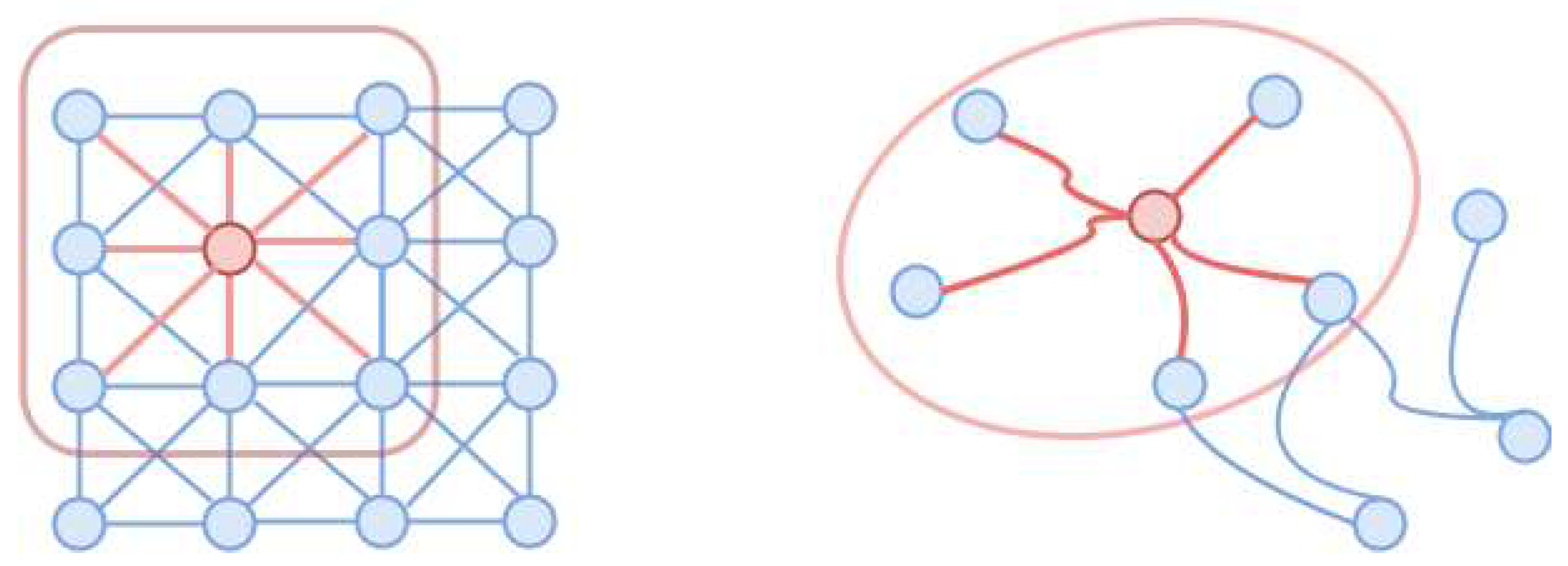
As briefly discussed in Section 2.5, inspired by the success of Convolutional Neural Networks, people attempted to generalize the convolution operation to graph-structured data. This genre of graph neural networks based on graph convolution operations is often referred to as Convolutional Graph Neural Networks (ConvGNNs); or simply as Graph Convolution Networks (GCNs). Akin to convolutional layers used in CNNs, a graph convolutional layer in GCNs generates higher-level representations of each graph node u by leveraging the information of its neighbourhood. However, as illustrated in Figure 7, unlike grid-like image data, which has a fixed and regular neighbouring structure, in a graph, a node’s neighbours are unordered and vary in size, which makes the generalization of the graph’s convolution operation much more challenging.

The first GCN proposed by Bruna et al. [29] is based on the spectral theorem, which uses graph Fourier transformation to transform the graph signal into its spectral domain, and then perform the graph convolution in that domain. Graph convolutions defined by the spectral method are closely related to filters in the context of graph signal processing, which can be interpreted as operations removing noise from the graph signals (or graph features in the context of graph representation learning) [29]. However, this method is computationally intensive since it requires calculating the graph Fourier transformation as well as the inverse graph Fourier transformation. Furthermore, the graph convolution relies on the eigen-decomposition of the Laplacian matrix, which implies that learnt convolution operations are domain-dependent and are not easily transferable to graphs with different topological properties [35].

ChebNet is then proposed to address those drawbacks [36], it uses Chebyshev polynomials to approximate the spectral graph convolution operation up to

k^{t h}

order. ChebNet implicitly avoids the graph Fourier transformation computation, thus reducing the computation complexity by a large margin.

Kipf and Welling further simplified the convolution operation in their work [5] by explicitly setting

k = 1

. Many later pieces of literature referred their model as GCN; thus, the same parlance will be adopted in the rest of this thesis.

GCN can be understood from the perspective of message passing, which has been introduced earlier in Section 2.5. Given a graph

G : = (V, E)

, and let

X \in R^{n \times (d + 1)}

be the feature matrix of G, whose the first column is 1 that reserved for bias terms in the weight matrix and whose

i^{t h}

row spanning from the 2^nd column to the

{(d + 1)}^{t h}

column is the transpose of the feature vector of node

v_{i}

. To obtain a high level representation

h_{i}^{(k)}

of node

v_{i}

at the

k^{t h}

GCN layer, an intermediate representation

m_{i}^{(k)}

is generated first by aggregating the representation of

v_{i}

’s neighbouring nodes and its own representation

h_{i}^{(k - 1)}

generated by the previous layer. This intermediate representation

m_{i}^{(k)}

is then transformed into the output representation

h_{i}^{(k)}

with a one hidden layer MLP.

The above process of node representation generation can be expressed in the matrix form as the following:

H^{(k)} = f (\tilde{A} H^{(k - 1)} W^{(k)})

(3.1)

where

H^{(k - 1)} \in R^{n \times (d_{k - 1} + 1)}

is the node representation matrix at the

{(k - 1)}^{t h}

GCN layer (an extra dimension for the bias term), such that its

i^{t h}

row is the transpose of the node representation vector

h_{i}^{(k)}

of node

u_{i} \in V

, the matrix

\tilde{A} : = A + I_{n}

is the adjacency matrix with self-loops added in,

W^{(k)} \in R^{(d_{k - 1} + 1) \times (d_{k} + 1)}

is a learnable weight matrix (note that here we shall use

{(W^{(k)})}^{T}

instead of

W^{(k)}

if we consider notation consistency with Chapter 2. But for simplicity we use the latter.) and

f (\cdot)

is an element-wise non-linear activation function. As usual, we take the initial

H^{(0)} = X

One issue with the above expression is that

\tilde{A} H^{(k - 1)}

is not normalized. This may introduce numerical instability and cause the exploding/vanishing gradient problem (e.g. nodes with many neighbours will get tremendous values in their representations) when multiple GCN layers are stacked together [5]. The most trivial solution to fix the issue is to modify (3.1) as follows:

H^{(k)} = f ({\tilde{D}}^{- 1} \tilde{A} H^{(k - 1)} W^{(k)})

(3.2)

where

\tilde{D} : = D + I_{n}

, and

D

is the degree matrix of the graph G. Adding the term

{\tilde{D}}^{- 1}

into (3.1) is equivalent as applying the mean operation, which normalizes each row of

\tilde{A}

based on the degree of nodes involved in. The node-wise message passing rule of (3.2) can be expressed as:

{h_{i}}^{(k)} = f (\sum_{j : v_{j} \in {N (v_{i}), v_{i}}} \frac{1}{(| N (v_{i}) | + 1)} {(W^{(k)})}^{T} {h_{j}}^{(k - 1)})

where

{({h_{i}}^{(k)})}^{T}

is the

i^{t h}

row of of the representation matrix

H^{(k)}

In the GCN model proposed by Kipf and Wellington [5], a more sophisticated normalization method, namely the symmetric normalization, is adopted:

H^{(k)} = f ({\tilde{D}}^{- \frac{1}{2}} \tilde{A} {\tilde{D}}^{- \frac{1}{2}} H^{(k - 1)} W^{(k)})

(3.3)

and the equivalent node-wise expression can be written as:

{h_{i}}^{(k)} = f (\sum_{j : v_{j} \in {N (v_{i}), v_{i}}} \frac{1}{\sqrt{(| N (v_{i}) | + 1) (| N (v_{j}) | + 1)}} {(W^{(k)})}^{T} {h_{j}}^{(k - 1)})

The utilization of symmetric normalization allows the definition of a more refined aggregation process, as this no longer amounts to the simple averaging of neighbouring nodes. However, both the normalized and symmetric normalized GCN models require prior knowledge of the entire graph structure to perform message passing, which makes them less robust and inapplicable to inductive-learning tasks (see Section 4.4 for more deatils). GraphSAGE [3] addressed this issue by introducing a general inductive framework, which samples a fixed-size set of neighbours of each node and only uses them to aggregate information in the message-passing step. The node representation generated by GraphSAGE can be expressed as:

h_{u}^{(k)} = f ({(W^{(k)})}^{T} {AGGREGATE}_{k} (h_{u}^{(k - 1)}, {h_{v}^{(k - 1)}, \forall v \in S_{N (u)}})

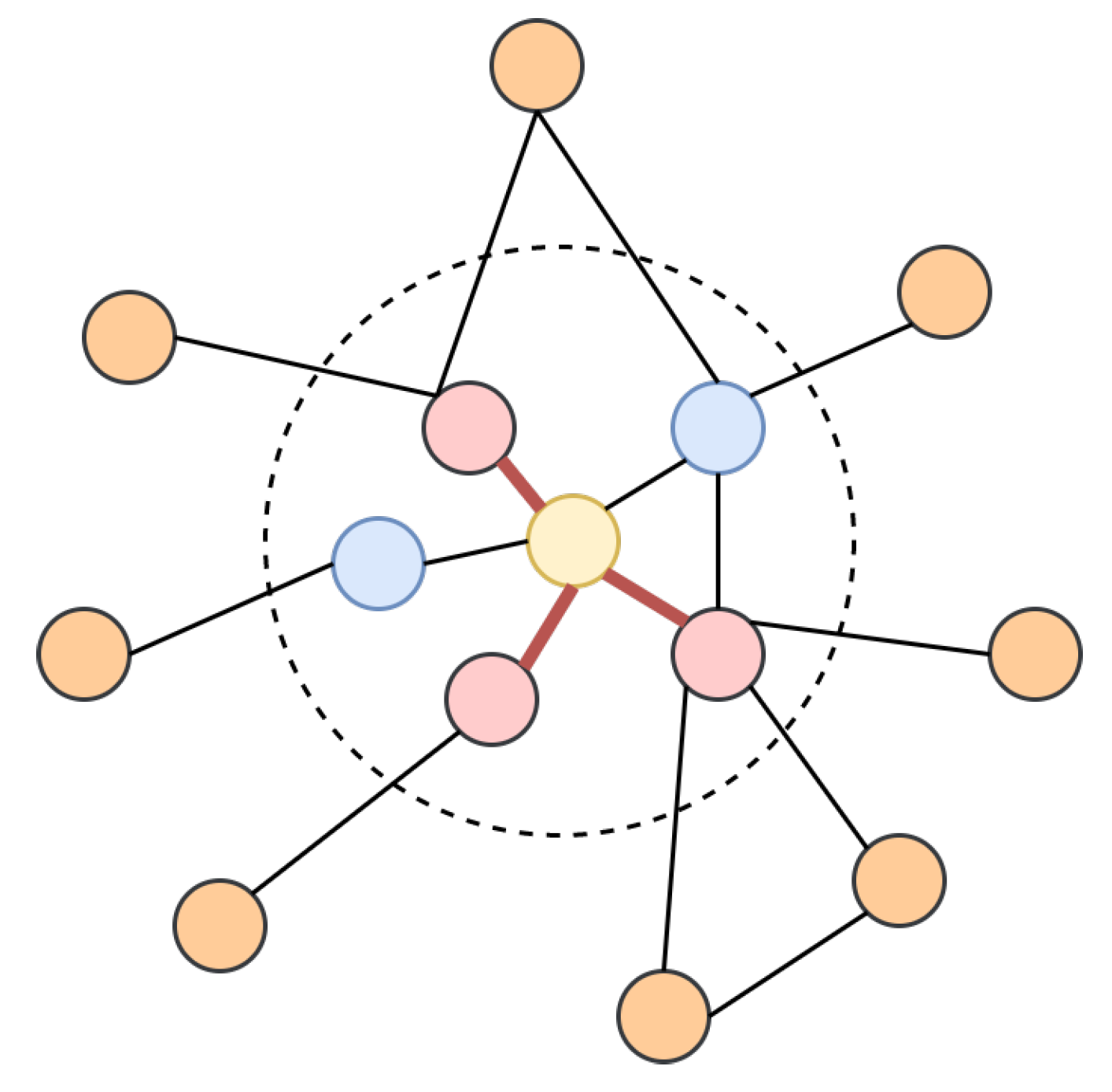
where

S_{N (u)}

is a random sample of the neighbours of node u, and

{AGGREGATE}_{k} (\cdot)

is the

A G G R E G A T E

operation at

k^{t h}

layer. Figure 8 shows an example of nodes sampled (red nodes) for the centering yellow node in its neighbourhood.

3.2. Attention Mechanism

The idea of attention was first proposed in the field of psychology, which is used to explain the cognitive process of selectively processing certain information in an environment while ignoring others [37]. Bahdanau et al. [38] were the first researchers who utilized the attention mechanism in machine learning; more specifically, they applied it to the machine translation task in natural language processing [39]. After their enormous success, people began to adopt and integrate the attention mechanism into different sub-domains of machine learning, such as computer vision [40] and recommendation systems [41]. Nowadays, the attention mechanism has became a prevailing concept in machine learning and it is also an essential component of many neural network architectures.

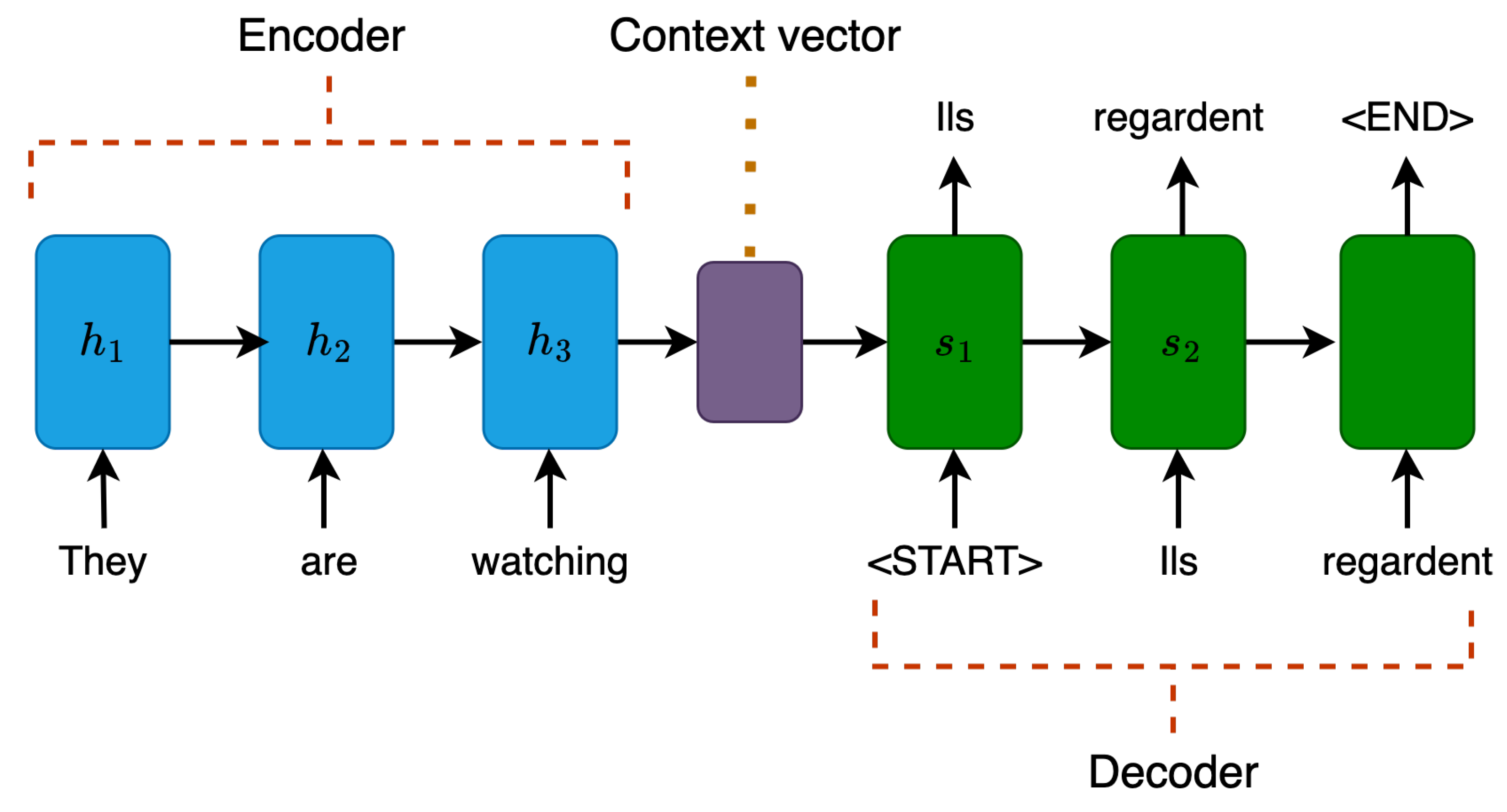
Before the attention mechanism was used for language modelling, the predominant architecture for natural language processing tasks was the sequence-to-sequence model (or the seq2seq model in short) [42]. The seq2seq model consists of two main components: an encoder and a decoder, which both are recurrent neural networks introduced in Section 2.4. With this specialized architecture, a seq2seq model can transform an input with an arbitrary length into an output with an arbitrary length. In particular, the encoder compresses the input sequence of tokens/words into a single fixed-length context vector, which then serves as the decoder’s input and is used to generate the output sequence. Figure 9 shows a high-level overview of a seq2seq model that translates the English sentence "They are watching" into the French sentence "Ils regardent".

Regardless of its prevalence, the traditional seq2seq model faced two major challenges. [39]. The first challenge is dealing with long input sequences; since the context vector generated by the encoder is fixed-length regardless of the input sequence size, this may lead to information loss when the input sequence is long [43]. The second challenge is to model alignment between the input and the output sequences, which is essential for certain tasks, such as machine translation and summarization. Intuitively speaking, in sequence-to-sequence tasks, each output token should be more influenced by certain parts of the input sequence than the rest. As an example, for the English-French translation showed in Figure 9, "Ils" in the output sequence should be associated with "They" in the input sequence, while "regardent" should be related to "are watching". Unfortunately, the encoder-decoder architecture utilized in the seq2seq model lacks any mechanism to selectively focus on relevant input tokens while generating each output token [44].

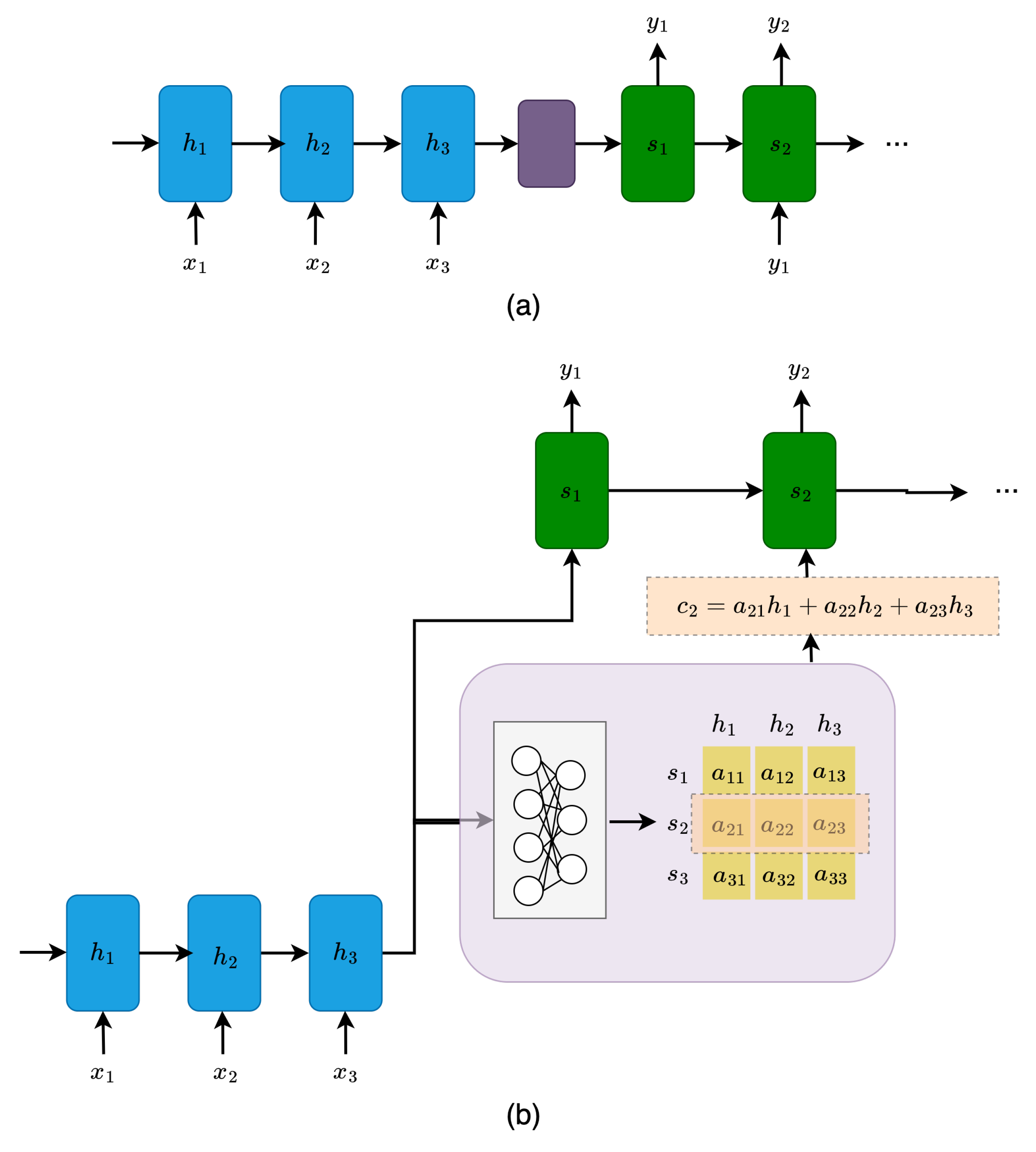
The attention model was proposed to mitigate those two challenges. The fundamental idea behind it is that, instead of generating the context vector solely based on the last hidden state of the encoder, attention weights, which reflect the inter-relationships between each pair of tokens in the input sequence, are used in lieu of in the context vector generation.

The attention weights are learned jointly with all the other model parameters during the training (by using a MLP). Next, the context vector is computed as the weighted sum of the encoder’s hidden states on all input tokens to avoid information loss. Then, when generating the output sequence, the attention weights prioritize a set of positions in the input sequence where the relevant information presents [39]. Figure 10 compares the traditional encode-decoder seq2seq architecture with the attention-based seq2seq architecture.

Even though the attention mechanism boosts the performance of the seq2seq model in many language-related tasks, it still has some drawbacks inherited from the recurrent architecture. One of the drawbacks is computational efficiency. It is difficult to parallelize the input sequence processing since the tokens are processed sequentially. [39]. Another flaw the seq2seq model has is its lack of ability to relate the tokens within the input/output sequence itself. To address these problems, Vaswani et al. proposed the Transformer architecture in [45], which profoundly impacted the later research of neural network architecture. In short, the Transformer eliminates the sequential processing and the recurrent architecture by utilizing the self-attention mechanism, allowing the model to see the entire input sequence simultaneously.

As hinted by its name, self-attention is an attention mechanism that computes a representation of a sequence by relating tokens at different positions of a sequence itself. The results in [45] revealed that the Transformer achieves higher accuracy with less training time via parallel processing for the machine translation task without using any recurrent component [39]. Apart from self-attention, another essential mechanism introduced in [45] is the multi-headed attention. Instead of computing the attention only once, the multi-headed mechanism runs through the attention computation multiple times in parallel by using different linear transformations of the same input sequence. The outputs are then concatenated and linearly transformed into the expected dimension [39]. The empirical results have shown that the attention weights learned using the multi-headed mechanism can even further boost the model’s performance.

3.3. Graph Attention Network

As mentioned in the preceding section, the attention mechanism frees the transformer model from the sequential processing of the input; this characteristic allows the idea to be easily extended to data structures other than a sequence, such as graph-structured data.

The graph-structured data extracted from the real-world are often large and chaotic; using attention can help highlight elements of the graph that are more relevant to the main task. Moreover, the attempt that forces the model to focus on the most important part of the graph potentially allows it to filter out the noises, thus improving the signal-to-noise ratio [46]. Another benefit of using attention is interpretability; the learned attention weights are a potential tool that may be used to interpret the results obtained from the model [47]. The attention mechanism on a graph can be defined at different levels, namely the node level, edge level, or sub-graph level; in this thesis, the focus will be on the node-level attention mechanism.

Given a graph

G : = (V, E)

, let node

v_{i} \in V

and let

N (v_{i}) \subseteq V

be the set of neighboring nodes of

v_{i}

. The attention on graph is defined as a function

f : v_{i} \times N (v_{i}) \to [0, 1]

that maps the node

v_{i}

and any node in

N (v_{i})

to a relevance score, which defines how much attention the target should give to each of its neighbor. Moreover, it is often assumed that

\sum_{v_{j} \in N (v_{i})} f (v_{i}, v_{j}) = 1

[48].

Several different types of graph attention mechanisms exist, though they all share the same principle and only differ in how the attention function f is defined.

One may quickly realize some similarities between the attention mechanism and the symmetric normalized adjacency matrix used in GCN ((3.3)). Both of them seem to be used to indicate the strength of relationship between a pair of connected node. Intuitively speaking, the elements in the symmetric normalized adjacency matrix can be viewed as a relevance score that are used to determine the importance of a given node and its neighbouring nodes during the message passing. The most significant distinction between the relevance score used by the two models is that the edge weights in the attention mechanism are learnt implicitly during the training.

The graph attention network (GAT) [4] extends the GCN by leveraging an explicit self-attention mechanism. As the name suggests, GAT introduces the attention mechanism when aggregating the neighbouring nodes’ features to substitute the normalized convolution operation. How important a node is to another node is determined jointly with other parameters during the training.

Let

v_{i}

and

v_{j}

be two connected nodes of G, and let

h_{i}^{(k - 1)} \in R^{d_{k - 1} + 1}

and

h_{j}^{(k - 1)} \in R^{d_{k - 1} + 1}

, respectively denote the representation vector of the nodes generated by the

{(k - 1)}^{t h}

layer. In particular, at the

k^{t h}

GAT layer, the amount of the attention node

v_{i}

should give to node

v_{j}

based on their representation vectors is computed via a shared attention mechanism att as:

where

W^{(k)} \in R^{(d_{k - 1} + 1) \times (d_{k} + 1)}

is a learnable weight matrix shared over all nodes.

In different variations of the GAT mode,

r_{i j}^{(k)}

is computed differently. In the original GAT, the attention mechanism is a one-layer MLP parameterized by a weight vector a ∈

R^{2 (d_{k} + 1)}

, and applying the the LeakyReLU non-linearity:

(3.4)

Brody et al. proposed GATv2 in [49], which modifies the original GAT model by defining

r_{i j}^{(k)}

as:

(3.5)

In particular, if we let

a^{(k)} : = [a_{1}^{(k)} | | a_{2}^{(k)}]

; since a^(k) is shared across all nodes in a graph, then in GAT, if there exists a node

v_{j_{\max}}

such that

{(a_{2}^{(k)})}^{T} {(W^{(k)})}^{T} h_{j_{\max}}^{(k - 1)}

is maximal among all the nodes, then for every

v_{i}

, the node

v_{j_{\max}}

will always obtain the highest attention score. As shown in (3.5), the GATv2 model alleviates the problem by making a^(k) non-global. As shown in (3.4), the first step performed in GAT is to transform the feature vectors by

{(W^{(k)})}^{T}

linearly, then two transformed vectors are concatenated and mapped by

{(a^{(k)})}^{T}

to an attention score

r_{i j}^{(k)}

GAT adopts masked attention to preserve the structural information - the attention scores are only computed between a node and its neighbouring nodes (i.e., in other words, GAT only computes

r_{i j}^{(k)}

between nodes

v_{i}

and

v_{j} \in N (v_{i})

), whereas in the most general form of graph attention, every pair of nodes can be attended to each other, which implies the graph structure is dropped completely. In particular, we use mask matrix M to enforce the structural information of the input matrix. The most commonly used mask matrix is defined by converting the zero-entry in the adjacency matrix into

- \infty

, i.e.

m_{i j} : = \{\begin{matrix} 0, & e_{i j} \in E \\ - \infty, & otherwise \end{matrix}

Let

R^{(k)} = (r_{i j}^{(k)})

denote the matrix of raw attention scores at the

k^{t h}

layer. To enforce the graph structural information into

R^{(k)}

, we update it by using M:

{\tilde{R}}^{(k)} = R^{(k)} + M

. Thus,

{\tilde{r}}_{i j}^{(k)} : = \{\begin{matrix} r_{i j}, & e_{i j} \in E \\ - \infty, & otherwise \end{matrix}

Furthermore, in order to make the computed attention scores to be easily comparable across different nodes, they are normalized by using the softmax function:

α_{i j}^{(k)} = {(softmax ({\tilde{R}}_{i :}^{(k)}))}_{j} = \frac{\exp ({\tilde{r}}_{i j}^{(k)})}{\sum_{k = 1}^{n} \exp ({\tilde{r}}_{i k}^{(k)})} = \frac{\exp ({\tilde{r}}_{i j}^{(k)})}{\sum_{k : v_{k} \in {N (v_{i}), v_{i}}} \exp (r_{i k}^{(k)})}

(3.6)

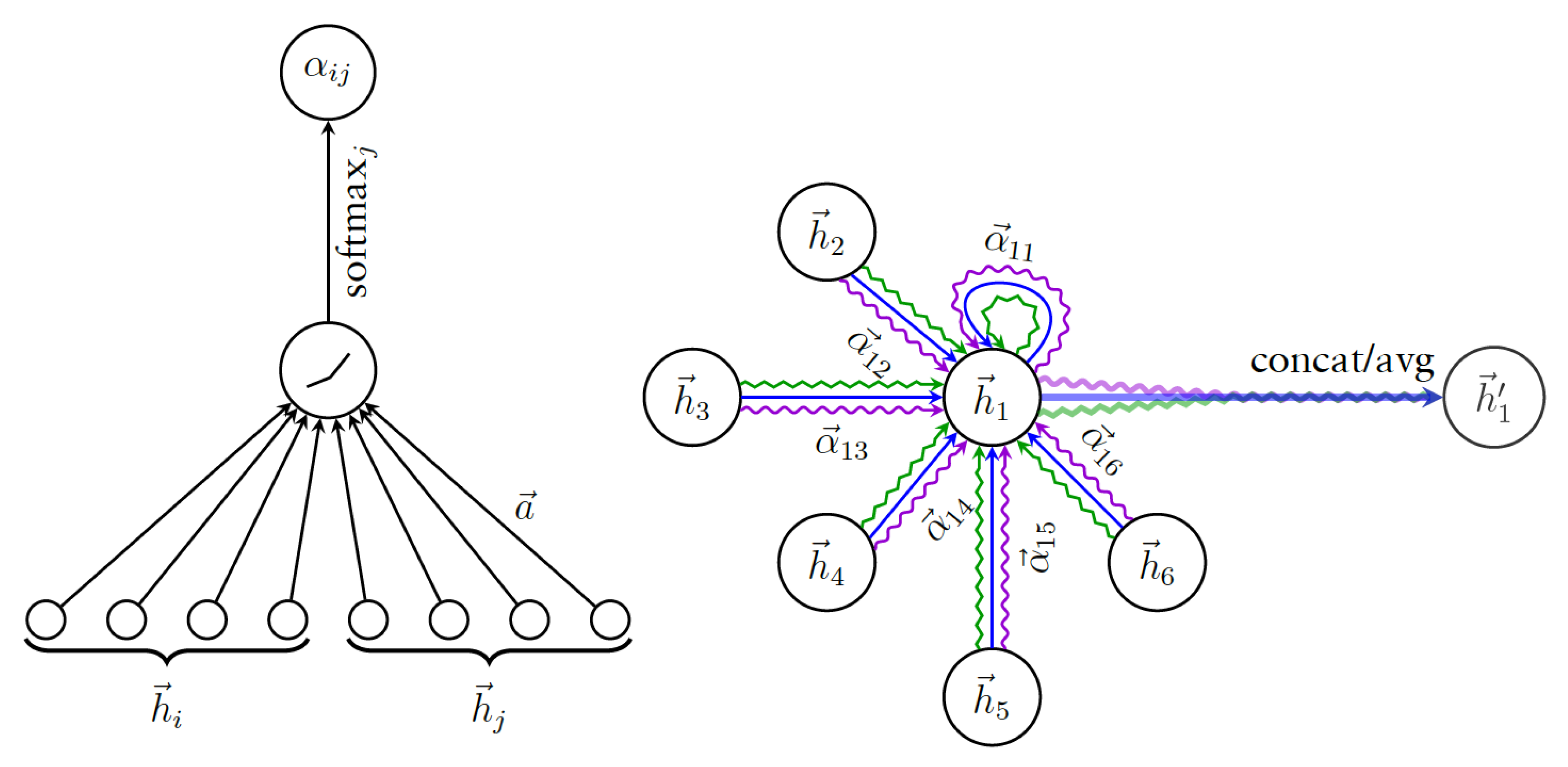
After applying the softmax function, all attention scores

α_{i j}^{(k)}

will be in range

[0, 1]

. This process is illustrated in Figure 11 (left).

Once the attention scores of node

v_{i}

and its neighbouring nodes are obtained, a new representation

h_{i}^{(k)}

of node

v_{i}

can be computed by:

h_{i}^{(k)} = f ({(W^{(k)})}^{T} \sum_{j : v_{j} \in {N (v_{i}), v_{i}}} α_{i j}^{(k)} h_{j}^{(k - 1)})

(3.7)

where

f (\cdot)

is a non-linear activation function and

h_{i}^{(k)}

is the aggregated representation for node

v_{i}

. This process is illustrated in Figure 11 (right).

The matrix form of (3.7) can be written as:

H^{(k)} = f (A_{att}^{(k)} H^{(k - 1)} W^{(k)})

where row i of

H^{(k)}

{(h_{i}^{(k)})}^{T}

and

A_{att}^{(k)}

is the attention matrix with

A_{att}^{(k)} (i, j) = α_{i j}^{(k)}

for

e_{i j} \in E

and 0 otherwise.

Alternatively, GAT utilizes a similar multi-head attention approach inspired by the transformer, which is a popular architecture in NLP [45]. Running multi-head attention is equivalent as running multiple attention mechanisms in parallel and aggregating the results. The multi-head attention allows the network to learn a richer representation of the input data and can help to stabilize the learning process of self-attention [4]. For example, M independent attention mechanisms are executed in parallel follows equation (3.7), and each of these attention mechanism is referred to as an “attention head”. The resulting representations are then concatenated to form the output feature representation:

(3.8)

where

α^{(k, m)}

is the normalized attention score computed by using the

m^{t h}

attention head at the

k^{t h}

layer, and

W^{(k, m)}

is the corresponding weight matrix. The matrix form of (3.8) can be written as:

Note that when multi-head attention is performed on the final layer of the network, concatenation no longer works, and averaging is employed instead:

or equivalently,

where K is the total number of GAT layers. Figure 11 illustrates the aggregation of a multi-head graph attention layer. Every neighbour i (as well as node 1 itself) of node 1 is associated with three attention score

{\bar{α}}_{1 i}

, which denoted by different colour lines in the figure. They are then been used to compute and aggregate the next level representation of node 1,

{\bar{h}}_{1}^{'} .

GAT has significantly outperformed GCN on the node classification task on several citation networks. However, recent studies [9,10,50] have shown that applying it or some other popular GNN architectures (including GCN) to heterophilous datasets can lead to significant performance loss.

3.4. Direction in Graph Neural Network

As mentioned in the preceding section, most GNNs choose between the mean, max or sum function as their AGGREGATE operation. However, this choice of AGGREGATE operation may lead to low discriminative power of GNNs, since all neighbours are treated equally [7]. Furthermore, some more serious issues that many GNNs suffered from could also be triggered by the utilization of such operations, namely the over-smoothing and over-squashing problems [51]. In particular, over-smoothing states the problem that node representations become indistinguishable as the number of layers in a GNN increases, whereas over-squashing refers to the lack of capability of GNN to propagate information between distant nodes effectively.

The most natural way to alleviate the aforementioned issues is by introducing a mechanism into the aggregation step to allow the model to distinguish messages passed from different neighbours. The GAT model introduced in the previous section adopts the attention mechanism based on the node features and utilizes attention scores to discern incoming messages. In particular, the weights defined by the node features can be considered as a form of the local directional flow that guides the message passing in the aggregation step [7]. In this section, we introduce the global directional flow over general graphs proposed by Beaini et al.’s [7].

3.4.1. Vector fields in a graph

In vector calculus and physics, a vector field is an assignment of a vector to each point in a subset of space. In order to establish the sense of direction in a graph, Beaini et al. [7] introduced the notation of vector field to a graph. Given a graph

G : = (V, E)

, define the vector space

L^{2} (V)

as the set of functions

V \to R^{n}

, along with

x

y \in L^{2} (V)

and scalar products:

< x, y >_{L^{2} (V)} : = \sum_{i : v_{i} \in V} x_{i} y_{i}

Similarly, the vector space

L^{2} (E)

is defined as the set of functions

E \to R^{n \times n}

with

F, H \in L^{2} (E)

, and scalar products:

< F, H >_{L^{2} (E)} : = \sum_{i, j : e_{i j} \in E} f_{i j} h_{i j}

Here

L^{2} (E)

can be regarded as the set of “vector fields” on the space

V

. For F

\in L^{2} (E)

, each row F

_{i, :}

represents a vector at node

v_{i}

and each element

f_{i j}

is a component of the vector going from node

v_{i} \in V

to node

v_{j}

through the edge

e_{i j}

. Note that

f_{i j} = 0

for nodes

v_{i}

and

v_{j}

that are not connected; furthermore, if no self-loops are added into the graph G,

f_{i i} = 0

for all nodes

v_{i} \in V

Let

| F |

denote the absolute value of F (i.e.,

| F | = (| f_{i j} |)

, and let

| | F_{i, :} {| |}_{L^{P}}

denote the

L^{P}

-norm of the i-th row of F. The positive/negative part of

F^{\pm}

then defines the forward/backward directional flow.

The pointwise scalar product is defined as the map

L^{2} (E) \times L^{2} (E) \to L^{2} (V)

, which takes two vector fields and returns their inner product at each node in

V

. The value at the node

v_{i}

is defined as:

< F, H >_{i} : = \sum_{j : v_{j} \in N (v_{i})} f_{i j} h_{i j}

The gradient ∇ of

x \in L^{2} (V)

is defined as a mapping

L^{2} (V) \to L^{2} (E)

{(\nabla x)}_{(i, j)} : = x_{j} - x_{i}

(3.9)

and the divergence div of F

\in L^{2} (E)

is defined as a mapping

L^{2} (E) \to L^{2} (V)

{(div F)}_{i} : = \sum_{j : v_{j} \in N (v_{i})} f_{i j}

(3.10)

Using (3.9) and (3.10), the directional derivative of the function

x \in L^{2} (V)

in the direction of the vector field

\hat{F}

can be defined as:

(3.11)

where each row of

\hat{F}

is the normalized by the

L^{1}

-norm:

for

i = 1, \dots, n

The directional derivative can be interpreted as the instantaneous rate of change of the function

x

moving through each node

v_{i} \in V

with velocity specified by

\hat{F}

3.4.2. Directional smoothing and derivatives operation

Now, we have defined the vector field F and established the sense of direction in graphs. In order to utilize those concepts to guide the information propagation in the graph, two weighted aggregation matrices, namely the directional average matrix

B_{av}

and the directional derivative matrix

B_{dx}

will be introduced.

The directional average matrix

B_{av}

is defined as

(3.12)

As shown in the above equation,

B_{av}

is a weighted aggregation matrix with non-negative weights; furthermore, all non-zero rows of

B_{av}

have their

L^{1}

-norm equal to 1. It assigns a large weight to the elements in the forward or backward direction of the field, while assigning a small weight to the other elements, with a total weight of one [7].

Let X

\in R^{n \times d}

(note that we omit the bias term here) denote the feature matrix of G, then its

m^{t h}

column

X_{:, m} \in R^{n}

is a vector consisting the

m^{t h}

features of all nodes in

V

, the directional smoothing aggregation at

X_{:, m}

is defined as

(3.13)

Note the

k^{t h}

element in

y_{m}

can be viewed as an weighted average over all the

m^{t h}

features of the neighbouring nodes of node

v_{k}

, more specifically, by the direction and amplitude of F.

The directional derivative matrix

B_{dx}

is defined as

(3.14)

The aggregator

B_{dx}

works by subtracting the projected forward message by the backward message (similar to a center derivative), with an additional diagonal term to balance both directions [7].

The directional derivative aggregation

y_{m}

of the

m^{t h}

feature vector

X_{:, m}

is defined as

(3.15)

which is essentially same as the centered directional derivative of

X_{:, m}

in the direction of

\hat{F}

. It is easy to show that (3.15) can also be expressed using (3.11):

(3.16)

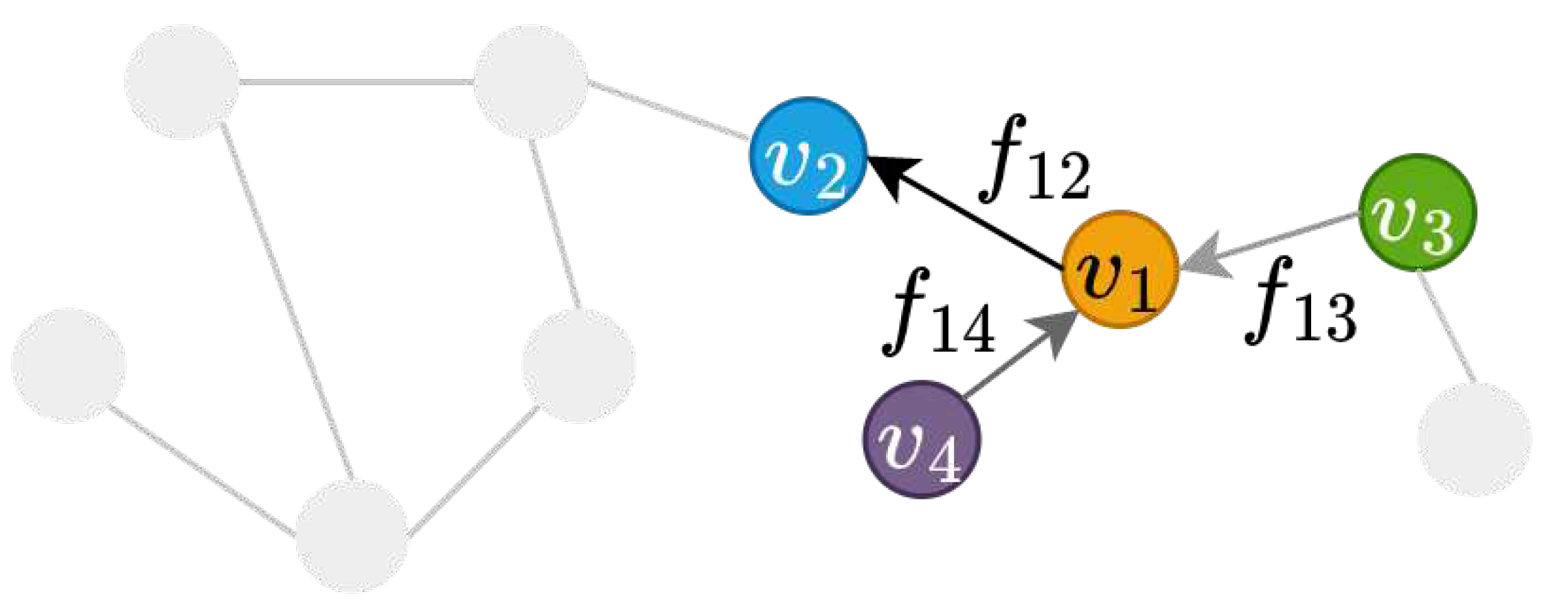
Figure 12 illustrates an example of how the directional aggregation works on a singe node

v_{1}

with three neighbouring nodes

v_{2}, v_{3}

and

v_{4}

Let

x_{1, m}, x_{2, m}, x_{3, m}

and

x_{4, m}

denote the

m^{t h}

feature of nodes

v_{1}, v_{2}, v_{3}

and

v_{4}

respectively. The directional smoothing aggregation

B_{av} {(F) X}_{:, m}

of the graph in Figure 12 centred at node

v_{1}

can be written as:

{(B_{av} {(F) X}_{:, m})}_{1} = \frac{| f_{12} | x_{2, m} + | f_{13} | x_{3, m} + | f_{14} | x_{4, m}}{| f_{12} | + | f_{13} | + | f_{14} |}

Similarly, the directional derivative aggregation

B_{dx} {(F) X}_{:, m}

of the graph in Figure 12 centred at node

v_{1}

can be written as:

{(B_{dx} {(F) X}_{:, m})}_{1} = \frac{| f_{12} | (x_{2, m} - x_{1, m}) + | f_{13} | (x_{1, m} - x_{3, m}) + | f_{14} | (x_{1, m} - x_{4, m})}{| f_{12} | + | f_{13} | + | f_{14} |}

where we assume

f_{12} > 0

f_{13} < 0

and

f_{14} < 0

3.4.3. Using gradient of the Laplacian eigenvectors as vector fields

With everything we have discussed in the preceding section, one may wonder what would be a reasonable choice of the vector field for general graphs. In [7], Beaini et al. proposed to use the gradient of low-frequency eigenvectors of the graph Laplacian as such vector field. The eigenvectors of the common types of Laplacian matrices (namely the unnormalized, degree-normalized and symmetric normalized Laplacian matrix) have been studied intensively in the field of spectral graph theory [52], and has been used extensively in the graph signal processing [53]. They are known to capture many imperative properties of graphs, thus making them a sensible choice for directional message passing (some theory is provided in Section 3.4.5).

In particular, if we let

ϕ^{(k)}

to denote the

k^{t h}

eigenvector of the Laplacian matrix of the input graph G, then its gradient is defined as:

\nabla ϕ_{i j}^{(k)} = \{\begin{matrix} ϕ_{i}^{(k)} - ϕ_{j}^{(k)}, & if e_{i j} \in E . \\ 0, & otherwise . \end{matrix}

(3.17)

3.4.4. Directional Graph Network

Based on the theoretical motivation discussed in the proceeding sections, Beaini et al. designed the Directional Graph Network (DGN), which utilizes directional smoothing and directional derivative aggregators in the message-passing step. In contrast to GAT and other previously mentioned message-passing GNNs, DGN demonstrates a distinct advantage over heterogeneous datasets due to its inherent anisotropic nature.

When utilizing the DGN model, there are two phases involved, namely the pre-computation phase and the GNN phase [7]. During the pre-computation phase, we compute the set of L eigenvectors

{ϕ^{(1)}, \dots, ϕ^{(L)}}

corresponding to the L smallest positive eigenvalues of the Laplacian matrix of the input graph. From now on, we denote the eigenvector associated with the eigenvalue

λ^{(k)}

ϕ^{(k)}

, i.e.,

L ϕ^{(k)} = λ^{(k)} ϕ^{(k)}

Then we calculated the gradients

{{\nabla ϕ}^{(1)}, \dots, {\nabla ϕ}^{(L)}}

of the eigenvectors as defined in (3.17). The computed gradients are then be used as the vector field, which we denoted by

F^{(k)}

. Lastly, we construct the directional smoothing aggregation matrix

B_{av}^{(k)}

and the directional derivative aggregation matrix

B_{dx}^{(k)}

for each

F^{(k)}

as shown in (3.12) and (3.14) respectively.

In the GNN phase, the DGN model takes the graph feature matrix

X \in R^{n \times (d + 1)}

, the adjacency matrix

A \in R^{n \times n}

, and the set of directional smoothing and directional derivative aggregation matrices

B = {B_{av}^{(1)}, B_{dx}^{(1)}, \dots, B_{av}^{(L)}, B_{dx}^{(L)}}

as inputs (where

B_{av}^{(k)} \in R^{n \times n}

and

B_{dx}^{(k)} \in R^{n \times n}

for each k). Then, the set of aggregation matrices

B

is used jointly with other aggregation operators, such as the simple mean operator

{\tilde{D}}^{- 1}

(same as the normalization operation used in the GCN introduced in Section 3.1), to aggregate the feature X of the input graph:

where

\hat{X} \in R^{n \times (2 L + 1) (d + 1)}

is the row concatenation of all directional and non-directional aggregation of the nodes features. Note that for the directional derivative aggregation operation

B_{dx}^{(k)}

, the absolute value is taken in order to avoid the sign ambiguity. Then similar to GCN, a one hidden layer MLP is applied to the aggregated node features generate the new representations of nodes:

H^{(1)} = f (\hat{X} W^{(1)})

where

W^{(1)} \in R^{(2 L + 1) (d + 1) \times d^{'}}

is a learnable weight matrix. Then at the

k^{t h}

DGN layer, the node representation matrix is computed as:

In the DGN model the number of eigenvectors to be used is regarded as a hyperparameter. However, Beani et al. showed both empirically and theoretically in [7] that taking the smallest non-trivial eigenvector is enough. Furthermore, the type of Laplacian matrix used by the DNG model is also a hyperparameter, where the options are

L

L_{rw}

and

L_{sym}

3.4.5. Theoretical Analysis

In this section, we review the theoretical analysis in [7], which justifies the choice of using the eigenvector

ϕ^{(1)}

corresponding to the smallest non-trivial eigenvalue

λ^{(1)}

of a graph Laplacian to define the global directional flow in a graph. This analysis also serves as an important theoretical foundation to our work in this thesis. The theorem in [7] states that by following the gradient of the eigenvectors, the diffusion distance between a pair of nodes on a graph could be reduced effectively.

Let

P = D^{- 1}

be the transition matrix (also called the random-walk matrix) of a j step Markov process on a graph

G : = (V, E)

, where the transition probability of graph nodes at each step is defined by

{P, P^{2}, \dots, P^{j}}

. Then the continuous time random-walk can be defined on the same graph, with the transition probability from node

v_{i}

to node

v_{j}

q_{t} (v_{i}, v_{j}) = \sum_{k = 0}^{\infty} \frac{e^{- t} t^{k}}{k!} p_{k} (v_{i}, v_{j})

(3.18)

where t represents continuous time and

p_{k} (v_{i}, v_{j}) : = P^{k} (i, j)

is the probability to transit from node

v_{i}

to node

v_{j}

in k steps. For instance, if

k = 1

, then

p_{1} (v_{i}, v_{j}) = \frac{1}{d_{i}}

e_{i j} \in E

and 0 otherwise. This transition probability is also referred to as the continuous heat kernel.

First, we outline the following lemma based on the results from [54].

Lemma 3.1.

The transition probability

q_{t} (v_{i}, v_{j})

of the continuous time random walk on graph can be written in the matrix form as:

Q_{t} = e^{- t (I - P)} = e^{- t L_{rw}}

where

Q_{t} (i, j) : = q_{t} (v_{i}, v_{j})

Next, we give the following definitions of diffusion distance and gradient step from [7].

Definition 3.1

(Diffusion distance). The diffusion distance at time t between the nodes

v_{i}

and

v_{j}

d_{t} (v_{i}, v_{j}) : = {(\sum_{m : v_{m} \in V} {(q_{t} (v_{i}, v_{m}) - q_{t} (v_{j}, v_{m}))}^{2})}^{\frac{1}{2}}

Note that the diffusion distance is small when there is high probability that the random walk starts in node

v_{i}

will meet the random walk starts in node

v_{j}

at time t. In graph representation learning, the diffusion distance is often used to model how node

v_{i}

influence node

v_{j}

[7].

Definition 3.2

(Gradient step). Let ϕ denote an eigenvector that corresponds to a non-trivial eigenvalue of a Laplacian matrix. Suppose that

ϕ_{m} - ϕ_{i} = \max_{j : v_{j} \in (v_{i})} (ϕ_{j} - ϕ_{i})

then we will say

v_{m}

is obtained from

v_{i}

by taking a step in the direction of the gradient of ∇ϕ

Lastly, we outline [7], Theorem 2.3 here.

Theorem 3.1

(Gradient steps reduce diffusion distance). Let

v_{i}

and

v_{j}

be two nodes such that

ϕ_{i}^{(1)} < ϕ_{j}^{(1)}

, where

ϕ^{(1)}

is the eigenvector corresponds to the smallest non-trivial eigenvalue

λ^{(1)}

L_{rw}

. Let

v_{m}

be the node obtained from

v_{i}

by taking one step in the direction of

\nabla ϕ^{(1)}

(as defined in the Definition 3.2). Then there is a constant C such that for

t \geq C

d_{t} (v_{m}, v_{j}) < d_{t} (v_{i}, v_{j})

with the reduction in distance being proportional to

e^{- λ^{(1)}}

The theorem presented in [7] considers only the eigenvector

ϕ^{(1)}

L_{rw}

for the DGN model. However, besides

L_{rw}

, [7] also utilized the eigenvectors from two other Laplacian matrices, namely

L

and

L_{sym}

, in their experimental setting. In particular, DGN using direction defined by the eigenvector of

L

corresponding to the smallest non-trivial eigenvalue yielded the best results (though this is not showing directly in [7], the choice of hyperparameters can be found in the authors’s github repository [55]). Therefore, it is imperative to extend the theorem to encompass the case that

L

is used.

4. Directional Graph Attention Network

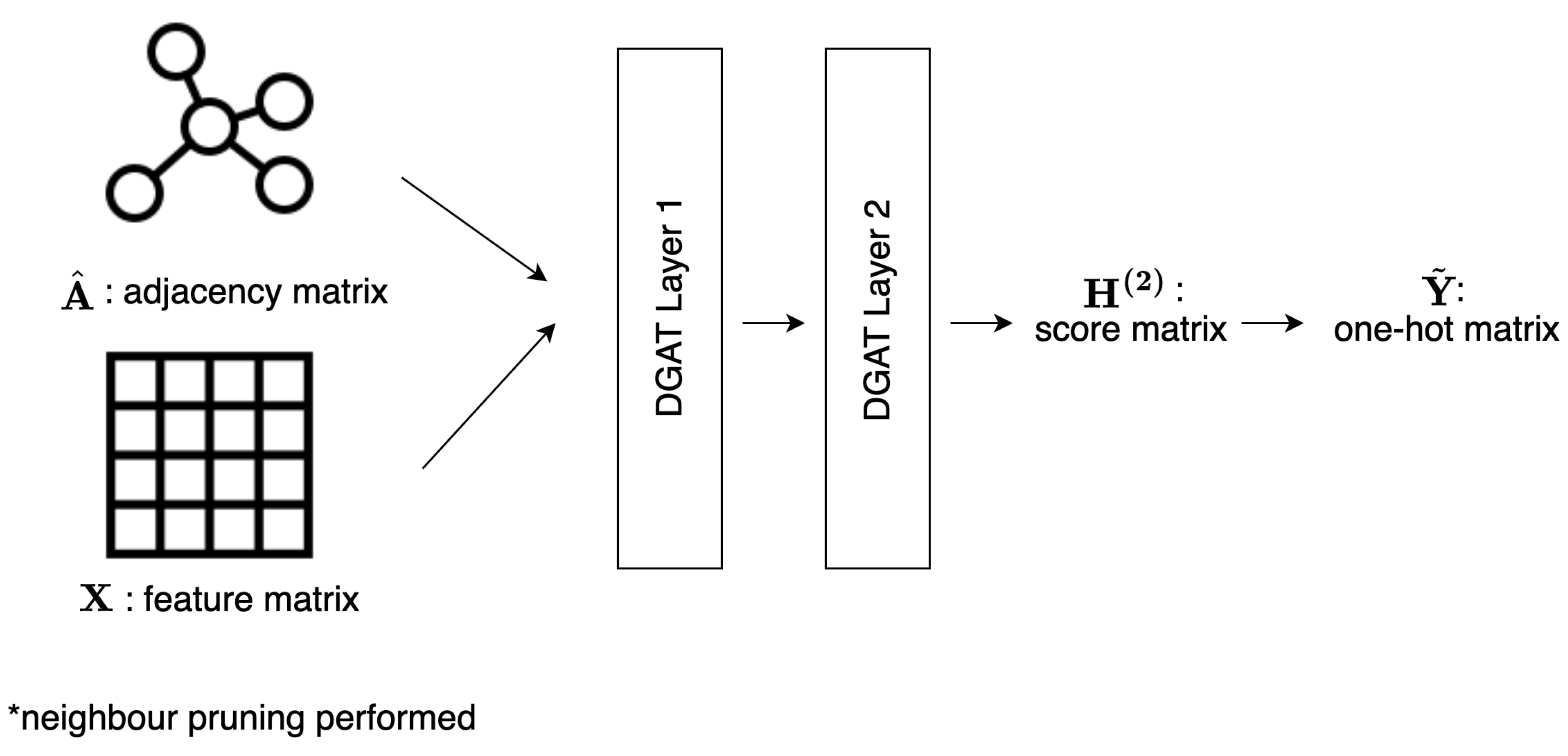
In this chapter, we propose our model, Directional Graph Attention Network (DGAT), which aims to enhance the performance of the original Graph Attention Network (GAT) on heterophilous datasets (verified empirically using node classification tasks). We introduce the global directional flow to the model, which is defined based on the vector field utilizing the low-frequency Laplacian eigenvector. More specifically, two new mechanisms are introduced on top of the original GAT architecture: the neighbour pruning and the global directional aggregation mechanism.

In Section 4.1, a formal statement of the problem is outlined. Next, our purposed DGAT model is described in Section 4.2 in detail. Lastly, the implementation, training and inference details of the DGAT model are outlined in Section 4.3, Section 4.4and Section 4.5 respectively.

4.1. Problem Statement

Let

G = (V, E)

be an undirected graph with

n = | V |

nodes. Let

A \in R^{n \times n}

and

D \in R^{n \times n}

denote the adjacency matrix and the degree matrix of G, respectively, and let

X \in R^{n \times d}

denote the feature matrix of nodes, where d is the number of features for each node. Our goal is to generate node representations that can be used for down-streaming tasks.

4.2. Methodology

As briefly mentioned in the proceeding chapter, the GAT model suffers significant performance lose when applying to heterophilous datasets [9,10,56]. In heterophily settings, the label

y_{u}

of and feature

x_{u}

of a node u might be very different from those its neighbours have. However, the GAT model generates the node representation solely based on the representations of its neighbours. While this might work well in the homophily case, where a node and its neighbours are likely to have the same label, a challenge is posed when the input graphs are heterophilic [57].

In this thesis, we propose the Directional Graph Attention Network (DGAT) to better guide the information propagation during the message passing, which aims to alleviate the aforementioned issue that the original GAT model has by exploiting both the local feature-based information and the global topology-based directional flow.

More specifically, the local feature-based message aggregation is accomplished by utilizing the standard attention mechanism in GAT, as introduced in Section 3.3. Therefore, we only need to design the global topology-based aggregation strategy, which should be flexible and can be easily integrated with the original GAT.

In this section, the two mechanisms, namely the neighbour pruning and the global directional aggregation mechanism, which our model utilizes to achieve the global topology-based directional aggregation, are outlined in detail.

Similar to the DGN model, two phases are involved while using the DGAT model: the pre-computation phase and the GNN phase. In the pre-computation phase, the eigenvector

ϕ^{(1)}

associated with the smallest non-trivial eigenvalue of a graph Laplacian matrix is computed, which is then used to define the vector field used by neighbour pruning and attention head mechanisms. Specifically, the gradient

{\nabla ϕ}^{(1)}

of the eigenvector

ϕ^{(1)}

is computed using (3.17) and the vector field is defined as

F : = {\nabla ϕ}^{(1)}

(4.1)

Here the Laplacian matrix we use is a new normalized Laplacian matrix, namely, the parameterized normalized Laplacian matrix, to be introduced in Section 4.2.3 Note that the DGN model uses one of the three graph Laplacian matrices introduced at the end of Section 3.4.4. The parameterized normalized Laplacian matrix has a parameter, which allows us to have a more refined control over the directional aggregation.

4.2.1. Neighbour pruning

Neighbour pruning is one of the two mechanisms that implement the global directional flow in our model. The intuition behind this mechanism is that we want to filter out the "noisy" (the nosiness is considered from the graph topology point of view) neighbours of a node and let it focus on the ones that carry the most important messages. More specifically, we consider neighbour pruning as a pre-processing step.

During neighbour pruning, for each node

v_{i} \in V

and its neighbouring node

v_{j} \in N (v_{i})

, we compare

| f_{i j} |

with a pre-defined threshold

ϵ

(note that F is defined in (4.1)). Then based on the homophily level of the input graph G, two different cases are considered: for homophilous G (i.e.,

H_{node} (G) \geq 0.5

; see (2.7)), we want to promote the neighbours with short diffusion distance, which have high probability sharing the same class labels [58], so if

| f_{i j} | < ϵ

, two actions are taken: first we remove the the edge

e_{i j}

between

v_{i}

and

v_{j}

, then, we set

f_{i j} = 0

; on the contrary, for heterophilous G (i.e.,

H_{node} (G) < 0.5

), we want to promote neighbours with long diffusion distance, which have higher probability of having different neighbours [58], so we proceed with the same two actions if

| f_{i j} | \geq ϵ

. This mechanism acts as graph denoising for the input graphs with different homophily levels, which forces the later aggregation step to focus on the appropriate set of neighbours. Note that we treat

ϵ

as a hyperparameter, and it is tuned independently for different datasets; a qualitative guidance on hot to narrow down the hyperparameter search range is provided in Chapter 5. Furthermore, since we are interested in the message passing in both the forward and the backward directions, the absolute value is taken. After performing neighbour pruning on the input graph, the re-wired graph is used in training.

An earlier edge-dropping mechanism was proposed in [59], where the edges of the input graph are dropped randomly during the training (similar to the dropout technique used in training an MLP, see more details in Section 4.4. Our proposed neighbour pruning mechanism differs from this mechanism fundamentally, we drop out graph edges in a guided manner, whereas the the aforementioned method is purely random. There also exists some other graph re-wring techniques. Papp et al. [60] proposed a node-dropping mechanism. Topping et al. [58] proposed a edge-adding mechanism in order to enhance the connectivity between poorly-connected clusters.

4.2.2. Global Directional Aggregation Mechanism

As mentioned in the preceding section, the original GAT utilizes multi-head attention to enrich the model’s capability and stabilize the learning process; more specifically, each attention head is feature-based, and completely omits the global topology.

To address this shortcoming, we propose two global directional aggregation mechanisms based on the directional weighted aggregation matrices

B_{av}

and

B_{dx}

defined in (3.12) and (3.14), respectively. In computing the two matrices, we use the vector field F defined in (4.1).

For a node

v_{i} \in V

, let

h_{i}^{(k - 1), av}

be its aggregated representation obtained by using the first global directional aggregation mechanism defined with

B_{av}

h_{i}^{(k - 1), av} = \sum_{j : v_{j} \in N (v_{i})} B_{av} (i, j) h_{j}^{(k - 1)}

(4.2)

where

f (\cdot)

is a non-linear activation function,

W_{av}

is the learnable weight matrix, and

h_{j}^{(k - 1)}

is the representation vector for node

v_{j}

at the

{(k - 1)}^{t h}

layer. Note that the initial representation vectors of the nodes used in the aggregation are just the node feature vectors. The equivalent matrix form can be written as:

H_{av}^{(k - 1)} = B_{av} H^{(k - 1)}

where the

i^{t h}

rows of

H^{(k - 1)}

and

H_{av}^{(k - 1)}

are

{(h_{i}^{(k - 1)})}^{T}

and

{(h_{i}^{(k - 1), av})}^{T}

, respectively.

Similarly, its aggregated representation

h_{i}^{(k - 1), dx}

by using the second global directional aggregation mechanism

B_{dx}

can be expressed as:

h_{i}^{(k - 1), dx} = \sum_{j : v_{j} \in N (v_{i})} B_{dx} (i, j) h_{j}^{(k - 1)}

The equivalent matrix form can be written as:

H_{dx}^{(k - 1)} = B_{dx} H^{(k - 1)}

To combine the global directional information with the feature-based attention heads, we can write the final representation of a node

v_{i}

produced by the

k^{t h}

DGAT layer as:

where M is the number of feature-based attention heads,

α_{i j}^{(k, m)}

is the normalized attention score between node

v_{i}

and

v_{j}

computed by the

m^{t h}

attention head at the

k^{t h}

DGAT layer (as defined in (3.6)) and

W^{(k, m)}

is the weight matrix corresponds to the

m^{t h}

attention head at the

k^{t h}

DGAT layer. The equivalent matrix form can be written as:

4.2.3. Parameterized normalized Laplacian and Adjacency Matrices

As briefly mentioned in the proceeding section, Beaini et al. [7] treat the type of Laplacian matrix (the choices being

L

L_{rw}

and

L_{sym}

) as a hyperparameter of the model and tune it for each individual benchmark. In order to gain a more refined control over the directional aggregation, we define a new class of Laplacian matrices, namely the parameterized normalized Laplacian matrix. In particular, this new class of the Laplacian matrix can be considered as a generalized version of the normalized Laplacian matrix as defined in (2.1). By using this new class of normalized Laplacian matrix (as defined in (4.3)) we introduce two parameters

γ

and

α

to the DGAT model, which control the eigenvalues and eigenvectors of the corresponding Laplacian matrix. Though not mentioned explicitly, the empirical results given in [55] showed that the model DGN using

L

has better performance than using

L_{rw}

and

L_{sym}

. Our newly defined class of Laplacian matrix will also help us to extend Theorem Section 3.4.5 to cover the case of

L

Definition 4.1

(Parameterized normalized Laplacian). A parameterized normalized Laplacian matrix is defined as

(4.3)

where the parameter

γ \in [0, 1]

and

α \in [0, 1]

Note that when

α = 0

and

γ = 1

L^{(α, γ)}

becomes the random-walk Laplacian L_rw, and when

α = \frac{1}{2}

and

γ = 1

L^{(α, γ)}

becomes the symmetric normalized Laplacian L_sym. Although we cannot choose

α

and

γ

such that

L^{(α, γ)}

becomes

L

, we have the following result:

(4.4)

This implies that when

γ

is small enough, an eigenvector of

L^{(α, γ)}

is a good approximation to an eigenvector of

L

Definition 4.2

(Parameterized normalized adjacent matrix). The parameterized normalized adjacent matrix corresponding to

L^{(α, γ)}

is defined as

P^{(α, γ)} : = I - L^{(α, γ)}

where the parameters

α, γ \in [0, 1]

When

α = 1

, the following result indicates

P^{(1, γ)}

is a valid random walk matrix.

Theorem 4.1.

The parameterized normalized adjacent matrix

P^{(α, γ)}

is non-negative (i.e., all of its elements are non-negative), and when

α = 1

P^{(α, γ)} 1 = 1

Proof.

By Definition 4.2, we have

It is easy to see that all elements in

P^{(α, γ)}

are non-negative. When

α = 1

P^{(α, γ)} = {(γ D + (1 - γ) I)}^{- 1} (γ + (1 - γ) I)

Since

A 1 = D 1

, we have

P^{(α, γ)} 1 = {(γ D + (1 - γ) I)}^{- 1} (γ + (1 - γ) I) 1 = 1

completing the proof. □

Next we study the properties of eigenvalues of

L^{(α, γ)}

in the following Lemma.

Theorem 4.2.

Suppose the graph

G = (V, E)

is connected. Let the symmetric

L^{(1 / 2, γ)} \in R^{n \times n}

have the eigendecomposition:

L^{(1 / 2, γ)} = U Λ U^{T}

where

Λ = (λ^{(i)} (γ))

with

λ^{(0)} (γ) \leq \dots \leq λ^{(n - 1)} (γ)

U \in R^{n \times n}

is orthogonal and its i-th column is an eigenvector corresponding to the eigenvalue

λ^{(i)} (γ)

. Then the eigenvalues have the following bounds:

0 = λ^{(0)} (γ) \leq λ^{(1)} (γ) \leq \dots \leq λ^{(n - 1)} (γ) \leq 2

(4.5)

where

λ^{(1)} (γ) \neq 0

, and

λ^{(i)} (γ)

is strictly increasing with respect to

γ

for

i = 1 : N - 1

. Furthermore,

L^{(α, γ)}

has the eigendecomposition

L^{(α, γ)} = ({(γ D + (1 - γ) I)}^{\frac{1}{2} - α} U) Λ {({(γ D + (1 - γ) I)}^{\frac{1}{2} - α}) U)}^{- 1}

i.e., all

λ^{(i)}

are also the eigenvalues of

L^{(α, γ)}

and the columns of

{(γ D + (1 - γ) I)}^{\frac{1}{2} - α}) U

are the corresponding eigenvectors.

Proof.

For any nonzero

x \in R^{n}

, write

y : = {(γ D + (1 - γ) I)}^{- 1 / 2} x

. Then

By the Rayleigh quotient theorem,

λ^{(0)} (γ) = \min_{y \neq 0} \frac{\frac{γ}{2} \sum_{i j} a_{i j} {(y_{i} - y_{j})}^{2}}{γ \sum_{i j} a_{i j} y_{i}^{2} + (1 - γ) \sum_{i} y_{i}^{2}} = 0

(4.6)

where the minimum is reached when

y = 1

and

\begin{matrix} λ^{(n - 1)} (γ) & = \max_{y \neq 0} \frac{\frac{γ}{2} \sum_{i j} a_{i j} {(y_{i} - y_{j})}^{2}}{γ \sum_{i j} a_{i j} y_{i}^{2} + (1 - γ) \sum_{i} y_{i}^{2}} \\ \leq \max_{y \neq 0} \frac{\sum_{i j} a_{i j} (y_{i}^{2} + y_{j}^{2})}{\sum_{i j} a_{i j} y_{i}^{2}} \leq 2 \end{matrix}

leading to (4.5).

The proof of showing

λ^{(1)} (γ) \neq 0

if and only if

G

is connected is similar to [61], Theorem 2.3, Corollary, thus we will omit the details here.

By the Courant-Fischer min-max theorem, for

γ \neq 0

It is obvious that the Rayleigh quotient

\frac{y^{T} L y}{y^{T} (D - I + (1 / γ) I) y}

is strictly increasing with respect to

γ \in (0, 1]

L y \neq 0

, i.e.,

y

not a multiple of 1. Note that

λ^{(0)} (γ) = 0

and it is reached when

L y =

0, or equivalently

y

is a multiple of 1. Thus,

λ^{(i)} (γ)

is strictly increasing with respect to

γ

for

i = 1 : n - 1

From the eigendecomposition of the symmetric

L^{(1 / 2, γ)}

, we can find the eigendecomposition of

L^{(α, γ)}

as follows: Preprints 84894 i025

Thus,

λ^{(i)}

is also an eigenvalue of

L^{(α, γ)}

for

i = 0 : n - 1

, and column i of

{(γ D + (1 - γ) I)}^{1 / 2 - α} U

is a corresponding eigenvector. □

Finally, we extend [7], Theorem 2.3 as follows.

Theorem 4.3

(Gradient steps reduce diffusion distance v2.) Let

v_{i}

and

v_{j}

be two nodes such that

ϕ_{i}^{(1)} (γ) < ϕ_{j}^{(1)} (γ)

, where

ϕ^{(1)} (γ)

is the eigenvector corresponds to the smallest non-trivial eigenvalue

λ^{(1)} (γ)

L^{(1, γ)}

. Let

v_{m}

be the node obtained from

v_{i}

by taking one step in the direction of

\nabla ϕ^{(1)} (γ)

(as defined in the Definition 3.2). Then there is a constant C such that for

t \geq C

d_{t} (v_{m}, v_{j}) < d_{t} (v_{i}, v_{j})

(4.7)

where

d_{t} (\cdot, \cdot)

is the diffusion distance between two nodes, as defined in Definition 3.1. With the reduction in distance being proportional to

e^{- λ^{(1)} (γ)}

Proof.

The proof is very similar to the proof of [7], Theorem 2.3. Let

p_{k} (v_{i}, v_{j}) = {(P^{(1, γ)})}^{k} (i, j)

, then

q_{k} (v_{i}, v_{j}) = \sum_{n = 0}^{\infty} \frac{e^{- t} t^{k}}{k!} p_{k} (v_{i}, v_{j})

, which is the transition probability from node

v_{i}

v_{j}

as defined in (3.18). The parameterized diffusion distance can be written as

d_{t} (v_{i}, v_{j}) : = {(\sum_{v_{m} \in V} {(q_{t} (v_{i}, v_{m}) - q_{t} (v_{j}, v_{m}))}^{2})}^{\frac{1}{2}}

(4.8)

By [54], we can rewrite (4.8) as:

d_{t} (v_{i}, v_{j}) = {(\sum_{k = 1}^{n - 1} e^{- 2 t λ^{(k)} (γ)} {(ϕ_{i}^{(1)} (γ) - ϕ_{k}^{(1)} (γ))}^{2})}^{\frac{1}{2}}

(4.9)

where

λ^{(1)} (γ) \leq λ^{(2)} (γ) \leq \dots \leq λ^{(n - 1)} (γ)

are eigenvalues of

L^{(1, γ)}

, and

{ϕ^{(1)} (γ), ϕ^{(2)} (γ), \dots, ϕ^{(n - 1)} (γ)}

are the corresponding eigenvectors. We omit

λ^{(0)} (γ)

since it equals to 0. The inequality

d_{t} (v_{m}, v_{j}) < d_{t} (v_{i}, v_{j})

is then equivalent as

(4.10)

We can take out

λ^{(1)} (γ)

and

ϕ^{(1)} (γ)

and rearrange the above inequality as:

(4.11)

Note that, the left-hand side of (4.11) is bounded above by:

Then (4.11) holds if:

(4.12)

which is equivalent to

(4.13)

Let the constant C be the left-hand side of (4.13), then if we take

t \geq ⌊C⌋ + 1

, we have

d_{t} (v_{m}, v_{j}) < d_{t} (v_{i}, v_{j})

. Note that C exits if

(4.14)

which requires

| ϕ_{i}^{(1)} (γ) - ϕ_{j}^{(1)} (γ) | > | ϕ_{m}^{(1)} (γ) - ϕ_{j}^{(1)} (γ) |

, and is based on the assumption that the chosen neighbor

v_{m}

v_{i}

always satisfies the condition that

ϕ_{i}^{(1)} (γ) < ϕ_{m}^{(1)} (γ) < ϕ_{j}^{(1)} (γ)

. However, it cannot be guaranteed that such neighbour

v_{m}

always exist, and this is indeed a shortcoming of this proof. □

The theorem presented in the original work [7, Theorem 2.3] (i.e., Theorem 3.1 in Section 3.4.5) provides justification solely for the direction utilized in the DGN model concerning the random walk matrix

L_{r w}

. However, our extended theorem given above significantly extends the scope of the original work by offering a theoretical justification for a much broader class of Laplacian matrices (as defined in Definition 4.1). Of particular note, we observe in (4.4) that as

γ

approaches zero, the eigenvectors of

L^{(1, γ)}

approach the eigenvectors of

L

, which provides strong evidence for the theorem’s asymptotic applicability to the unnormalized Laplacian matrix

L

Moreover, we can now provide theoretical justification for the empirical results observed in the experiments from [55], which demonstrate that defining directions in DGN by utilizing the eigenvectors of

L

leads to superior results as compared to using the eigenvectors of

L_{r w}

. As previously mentioned, the eigenvector

Φ^{(1)} (γ)

L^{(1, γ)}

corresponding to the eigenvalue

λ^{(1)} (γ)

converges to the eigenvector

Φ^{(1)} (0)

L

γ

approaches 0; furthermore,

L^{(1, γ)} = L_{r w}

when

γ = 1

. Based on Theorem 4.2, it can be inferred that for

γ \in (0, 1)

λ^{(1)} (γ)

is less than

λ^{(1)} (1)

, which implies

e^{- λ^{(1)} (1)} < e^{- λ^{(1)} (γ)}

. Moreover, by applying Theorem 4.3, we can infer the direction defined in DGN with the utilization of

Φ^{(1)} (γ)

is expected to result in a more significant reduction in diffusion distance when

γ

approaches 0. In other words, utilizing

Φ^{(1)} (γ)

to define direction in DGN will enable more efficient message passing due to the reduced diffusion distance.

Parameter

γ

and

α

affect the amount of diffusion distance reduction. Thus, by adding

γ

and

α

as a tunable hyperparameter to the DGAT model, we will be able to have finer control over the message aggregation. In Section 5.4.1, we provide qualitative guidance on choosing

γ

and

α

for different input graphs based on their heterophily level.

4.3. Vectorized Implementation

The DGAT model is constructed by stacking two directional attention layers, which is based on the standard graph attention layer with extra global directional information added in. We designed our model to have two directional attention layers for the sake of a fair comparison with the original GAT which usually works best with a couple number of layers. Figure 13 illustrates the overall structure of the DGAT model. More specifically, we use efficient matrix multiplications to implement it.

Suppose we have already performed the neighbour pruning on the input graph

G : = (V, E)

. Let

\hat{G}

denote the re-wired graph, and let

\hat{A}

, X represents its adjacency matrix and the node feature matrix respectively. As mentioned in the preceding section, in order to get the masked attention scores for the

m^{t h}

attention head at the

k^{t h}

DGAT layer, we need to first compute the matrix according to (3.4):

R^{(k, m)} = (r_{i j}^{(k, m)})

, which contains the unnormalized attention scores for all pairs of nodes in

\hat{G}

After we compute

R^{(k)}

, according to (3.6) we calculate the masked attention matrix score as

A_{att}^{(k, m)} = (α_{i j}^{(k, m)})

. Then the model can be written as follows:

Like the GAT model, our new model uses LeakyReLU as the activation function

f (\cdot)

in our implementation.

Note that in spite of the improvement made by GATv2 to the original GAT model, in our implementation, we still use the attention mechanism proposed in the GAT model for the following reasons:

The GAT model is the first graph model that adopts the attention mechanism. Although the GATv2 model is better, its attention mechanism is still feature-based and there is no essential difference between the two models.
The mechanisms we proposed are immune to the type of attention mechanisms they can combine with and can be used to enhance any attention mechanism.
The experiment results in Section 5.4.2 indicate that our DGAT model outperforms GATv2 by a large margin on all synthetic benchmarks. Thus, we believe that there will also be a significant enhancement when applying our mechanisms to the GATv2 model. We will leave the empirical experiments to future work

4.4. Training

To train and evaluate the DGAT model, we use various node classification benchmarks (see more details about benchmarks in Chapter 5).

More specifically, we assume a total of T classes of labels in a node classification task. A subset of the nodes

\tilde{V} \subset V

have labels

{y_{i} : v_{i} \in \tilde{V}}

associated with them, while the labels for the rest of the nodes are unknown. The focus of the task is to infer the labels for the nodes in

V ∖ \tilde{V}

. Note that it is a common practice to convert label

y_{i}

into one-hot vector

y_{i} \in R^{T}

, where the

k^{t h}

element of

y_{i}

is 1 if

y_{i}

indicates the node is in class k, and all the rest elements are 0. We also adopt this convention in our experiment.

When training and evaluating a model using a node classification benchmark dataset with T distinct classes, each node

v_{i} \in V

has a label vector

y_{i}

associated to it. Moreover, we divide nodes into three sets, namely the training set

V_{train}

, the validation set

V_{val}

and the test set

V_{test}

. During the training phase, the model only has access to labels of nodes in

V_{train}

and in

V_{val}

(for hyperparameter tuning), while the labels of the rest of the nodes in

V_{test} = V ∖ (V_{train} \cup V_{val})

remain unknown to the model.

The cost function used in node classification tasks is the standard categorical cross-entropy loss [14], which is commonly used for multi-class classification tasks:

C = - \frac{1}{| V_{train} |} \sum_{i : v_{i} \in V_{train}} y_{i}^{T} \log {\tilde{h}}_{i}^{(2)}

(4.15)

where

y_{i} \in R^{T}

is the one-hot encoding for the ground-truth class label of node v_i,

{\tilde{h}}_{i}^{(2)} = {(softmax (H_{i, :}^{(2)}))}^{T}

, and log(·) is applied element-wise.

In our experiment, we adopt the batch gradient descent method using the full training dataset in each training iteration. In addition, we introduce stochasticity into the training process by employing the dropout technique [62].

Dropout is a powerful regularization technique for general deep neural networks. Specifically, when training with dropout, every neuron (along with its connection) in the input and the hidden layers has a probability p of being dropped. The dropout probability p is considered as a hyperparameter which requires tuning for different datasets. Figure 14 illustrates how dropout works in a simple neural network with two hidden layer.

Dropout prevents neural network from over-fitting by forcing each neuron to not rely on the fixed set of neurons connected to it from the previous layer. As a result, the neural network is exposed to a wide variety of different contexts provided by the different hidden units and thus usually generalizes better to unseen data. Note that the dropout is only used during training and is turned off in the inference/test phase.

Another technique we adopted in the training process is the weight decay [63], which is a regularization technique that helps to reduce the complexity of a model and prevent overfitting. In particular, by using the weight decay technique, we modify the original cost function C by adding a penalty term that is proportional to the squared sum of the weights:

\tilde{C} = C + \frac{λ}{2} w^{T} w

where

λ

is the hyperparameter that determines the strength of the penalty and w is a vector containing all weights in the neural network.

Moreover, when training a graph neural network to generate node-level representations, there are typically two learning frameworks, which are

Transductive learning: The model has access to features of all the nodes during the training, including the nodes in $V_{test}$ . Note that the labels of nodes in $V_{test}$ are not visible to the model, and they are not used in the loss computation; however, the nodes in $V_{test}$ will be involved in the message-passing step, and the model will generate the intermediate representations for them.

and the

Inductive learning: The model only has access to features of nodes in $V_{train}$ and $V_{val}$ during training. In this case, the $V_{test}$ nodes are used in neither the loss computation nor the message-passing step; they are entirely invisible to the model.

In this thesis, we adopt the transductive learning framework in training the DGAT model.

4.5. Testing

After the model is trained (i.e., all the weights have been obtained), we compute the attention score matrix

H^{(2)}

of the input graph G. To predict labels for graph nodes in

V_{test}

, we convert the corresponding rows in

H^{(2)}

into a one-hot matrix that represents the node classification results. Specifically, to get a class label for node

v_{i} \in V_{test}

, we extract the

i^{t h}

row of

H^{(2)}

and find the index of the maximum score in it. Then we turn the element at this index into 1 and the rest of elements in the row vector into 0. By repeating this process for each node in the input graph, we convert

H^{(2)}

into a one-hot matrix

{\tilde{Y}}_{test}

, whose

i^{t h}

row in is the predicted one-hot vector label of node

v_{i} \in V_{test}

In order to test performance of our model, we calculate the average test accuracy against the ground-truth labels:

accuracy = \frac{1}{| V_{test} |} \sum_{i : v_{i} \in V_{test}} ind (y_{i} = {\tilde{y}}_{i})

where

(\cdot)

is the indicator function, which returns 1 if the classes match and 0 otherwise.

4.6. Summary

This chapter describes our proposed model, DGAT, which operates on graph-structured data, leveraging the graph topology-based directional flow into the standard graph attention mechanism. To demonstrate the effectiveness of the DGAT model, we conducted a series of experiments on different real-world and synthetic node classification benchmarks. The detail and results of our experimental study are presented in the next chapter.

5. Experimental Studies

This chapter examines the empirical behaviour of the proposed model, DGAT. We demonstrate the model’s effusiveness by evaluating its performance against various benchmarks. Specifically, we compare its results to those of the original GAT model and the DGN model across nine real-world datasets. Furthermore, we conduct an additional evaluation by comparing the model’s performance to GAT and GATv2 on ten synthetic datasets. This analysis allows us to gauge the model’s effectiveness in handling graphs that exhibit varying levels of heteroplicity.

In Section 5.1, the real-world datasets used in the experiment are introduced. Next, the synthetic datasets used in the experiment are presented in Section 5.2. Then in Section 5.3, our experimental setup is explained. Lastly, the test results are presented and discussed in Section 5.4.

5.1. Real-World Datasets

We utilized nine real-world node classification benchmarks in our experiment to evaluate the DGAT model. Those nine datasets can be categorized into four groups: the Wikipedia network, the actor co-occurrence network, the WebKB and the citation network. The overall statistics of the datasets are shown in Table 1. In the following sub-section, we give a thorough overview of each of them.

5.1.1. Wikipedia networks

The graphs of Wikipedia networks are collected from the English Wikipedia [64], each graph reflects the page-to-page referencing relationship on some specific topics (e.g. chameleons, crocodiles and squirrels). In our experiment, the two networks we used are the Chameleon and the Squirrel. The nodes in a Wikepedia network represent Wikipedia article web-pages and edges are mutual link between them. The features of the nodes represent the appearance of certain pre-defined informative nouns in the articles. The nodes are classified into five categories. Each category represents a range that the average monthly web page traffic falls into between October 2017 and November 2018.

5.1.2. Actor co-occurrence network

The graph Actor is a actor-induced subgraph of the film-director-actor-writer network [65]. The nodes in this graph represent actors, and an edge connecting two nodes indicates the co-occurrence of those two actors on the same Wikipedia page. The features of a node of the graph correspond to a set of specialized keywords on the Wikipedia pages. Moreover, the nodes are classified according to the words of the actors’ Wikipedia.

5.1.3. WebKB

WebKB [66] is a graph representing web pages collected from the computer science departments of various universities. In our experiment, three sub-datasets of it are used, namely Cornell, Wisconsin and Texas. The nodes in these networks represent web pages, and edges are hyperlinks between them. A node’s label is the web page’s categories (Student, Faculty, Staff, Department, Course and Project). The features of the nodes are bag-of-words representation (i.e.,

0 / 1

-valued word vector that indicates the absence/presence of the corresponding word from a vocabulary set) of the web pages.

5.1.4. Citation networks

Cora [67], Citeseer [68] and Pubmed [69] are three real-world benchmark datasets commonly used in node classification tasks. In all three of these networks, nodes represent papers, and edges between nodes indicate citations of one paper by another. The nodes have been assigned different labels according to the topic of the paper it represents. The features of the nodes are the bag-of-words representation of the paper and note that the stop-words and words that appeared less than ten times are removed from the feature vector to reduce noises.

5.2. Synthetic Datasets

In addition to the real-world datasets, we also tested the DGAT model on a set of synthetic graphs generated with different homophily levels ranging from 0 to 1 with the method proposed in [70].

More specifically, given the total number of nodes n we wish to have in the output graph G, the total number of classes T and the homophily coefficient

μ

; we first divide those n nodes into T equal-size classes. Then the output synthetic graph G (initially empty) is generated iteratively by adding a new node

v_{i}

with a random class label vector

y_{i}

at each step. Furthermore, whenever a new node

v_{i}

is added to the graph, we connect it to an existing node

v_{j}

in G with the probability

p_{i j}

defined by the following rules:

p_{i j} = \{\begin{matrix} d_{i} \times μ, & if y_{i} = y_{j} . \\ d_{j} \times μ \times w_{| c_{i} - c_{j} |}, & otherwise . \end{matrix}

(5.1)

where

y_{i}

and

y_{j}

are class labels of node u and v respectively, and

w_{| y_{i} - y_{j} |}

is the “cost” of connecting two distinct classes with distance

| y_{i} - y_{j} |

Specifically, the distance between two classes simply implies the shortest distance d between the two classes on a circle, starting from 1 to T respectively. For instance, if

T = 6

y_{i} = 1

and

y_{j} = 3

, then distance between

y_{i}

and

y_{j}

is 2.

Moreover, the cost

w_{d}

decreases exponentially with respect to the increase of distance d. For example, if

T = 6

and if we let

w_{| 1 - 4 |} = 1

(where distance

= 3

), then

w_{| 1 - 3 |} = w_{| 1 - 5 |} = 2

(where distance

= 2

) and

w_{| 1 - 2 |} = w_{| 1 - 6 |} = 4

(where distance

= 1

) [70]. Furthermore, we normalize the costs such that

\sum w_{| c_{u} - c_{v} |} = 1

In addition, we also normalize the probability

p_{i j}

defined in (5.1) over the exiting nodes when generating the synthetic graph, where:

{\bar{p}}_{i j} = \frac{p_{i j}}{\sum_{k : v_{k} \in N (v_{i})} p_{i k}}

Lastly, the features of each node in the output graph are sampled from a 2D Gaussian distribution, where each class has its own distribution defined separately.

5.3. Experimental Setup

As mentioned in Section 4.3, the DGAT model is constructed by using two directional attention layers. In addition, the model’s hyperparameters have been optimized for all datasets, including learning rate, weight decay, dropout rate, the neighbour pruning threshold

ϵ

(as introduced in Section 4.2.1), and

γ

in the parameterized random-walk normalized Laplacian (as defined in (4.3)). In addition, we use the Adam optimizer and the early stopping strategy during the training phase, which is the same as the training setting utilized in the GAT model [4]. The DGAT model also uses the same number of attention heads (8), the same number of graph attention layers (2) and the same number of initial hidden units (48 for Chameleon and Squirrel, 32 for Actor, 32 for Cornell, Wisconsin and Texas, 16 for Cora and Citeseer, and 64 for Pubmed) as the GAT model in [4].

Table 2 summarizes the fine-tuned hyperparameters of the DGAT model for each real-world dataset.

In our experiment, we utilize the geom-split strategy [34], which splits nodes in each class into

60 % - 20 % - 20 %

sets for training, validation and testing. Furthermore, we report the average test accuracies of all datasets over the ten random splits. Finally, to validate the effectiveness of the DGAT model, we establish the GAT and DGN models as baselines and compare DGAT’s performance against them across all datasets.

5.4. Results and Analysis

5.4.1. Real-world Dataset

We conducted experiments on node classification tasks to evaluate our proposed DGAT model. As mentioned earlier, we use GAT and the DGN as our baseline models.

Table 3 presents the average performance of our model on nine real-world datasets across ten random splits. The results illustrate the efficacy of our model, as it outperformed the original GAT on all nine datasets, particularly those with heterophilic characteristics. To be more specific, the DGAT model outperformed the GAT baseline model by a significant margin of

9.54 %

4.79 %

7.23 %

30.82 %

35.3 %

21.08 %

on the heterophilic datasets, namely, Chameleon, Squirrel, Actor, Cornell, Wisconsin and Texas; and by a relatively smaller margin of

1.68 %

2.09 %

0.31 %

on the homophilic datasets, namely Cora, Citeseer and Pubmed. These results suggest that incorporating global topological information into the attention mechanism do yield benefits, particularly for benchmark datasets with pronounced heterophilic characteristics.

In addition, the DGAT model outperforms the DGN baseline model by a margin of

1.99 %

0.21 %

8.11 %

1.96 %

1.35 %

on all the heterophilic datasets except Squirrel, namely, Chameleon, Actor, Cornell, Wisconsin and Texas; and by a margin of

3.36 %

2.54 %

3.64 %

on the homophilic datasets, namely Cora, Citeseer and Pubmed. As previously mentioned, the DGN model holds a significant advantage over the GAT model due to its inherent anisotropic nature. The experimental results provide further evidence supporting the effectiveness of incorporating the directional aggregation mechanism into the original attention mechanism for notable improvements. Furthermore, the DGAT model demonstrates superior performance compared to the DGN model across all homophilic datasets. This outcome serves as evidence that our proposed model effectively combines the advantages of both mechanisms.

In terms of the hyperparameter searching, based on our empirical experience, we advice to set the search range for

ϵ

between

10^{- 7}

10^{- 3}

, and search range for

α

between

0.1

0.9

. Moreover, the hyperparameter

γ

in Table 2 exhibits a correlation between the homophily level: the fine-tuned values of

γ

for strong homophily datasets appear to be larger than those strong heterophily datasets. This observation suggests that the homophily level of a graph may have an impact on the choice of

γ

for the DGAT model.

To assess the effectiveness and efficiency of our proposed model, we perform an ablation study to examine the impact of different mechanisms, namely the neighbor pruning, global directional aggregation, and the parameterized random-walk normalized Laplacian matrix. The study is aimed at evaluating the performance of the proposed framework in the context of the same real-world benchmark datasets, namely Cornell, Wisconsin, Texas, Film, Chameleon, Squirrel, Cora, Citeseer and Pubmed, using a

60 % / 20 % / 20 %

random split for train/validation/test. The results are reported in terms of the average test accuracy and standard deviation.

Ablation Tests

In this section, we present the results of an ablation study conducted on all nine real-world datasets using DGAT. As aforementioned, the purpose of this study is to assess the efficacy of each proposed mechanism. Table 4 displays the results obtained from the ablation tests.

The ablation test results suggest that the utilization of three proposed mechanisms, namely neighbor pruning, global directional aggregation, and parameterized random-walk normalized Laplacian matrix, enhances the efficiency of message passing. Additionally, similar to the previously mentioned observation, graphs exhibiting stronger heterophily characteristics experience greater benefits from the directional message passing approach. Furthermore, it is worth mentioning that the utilization of neighbor pruning in DGAT yields remarkable enhancements in its performance when applied to real-world datasets. These improvements contribute to the enhanced performance of the heterogeneous dataset, namely Chameleon, Squirrel, Actor, Cornell, Wisconsin, and Texas, resulting in performance gains of

20 %

9.59 %

23.87 %

51.25 %

69.84 %

and

34.26 %

respectively.

To further prove the effectiveness and investigate the underlying relationship between

γ

and the graph homophily level, we conducted more experiments by utilizing synthetic datasets in the next section.

5.4.2. Synthetic Dataset

We have shown promising results of our DGAT model on the real-world benchmarks. In this section, we conducted more experiments on the node classification task using ten synthetic graphs with homophily coefficients ranging from 0 to 0.9. Note that the correlation between the homophily coefficient and

H_{node}

is very close to linear, thus we use homophily coefficient directly in this section to represent the homophily level of the synthetic datasets.

Similar to the experiments run on real-world datasets, we use the original GAT model as our baseline. In addition, the GATv2 model is also used in the synthetic experiment to further demonstrate our model’s enhancement to the attention mechanism. The experiment results can be found in Table 5. In order to offer a more thorough depiction of the comparison between the models’ performances, we added Figure 15 to our presentation as well.

Being an important hyperparameter introduced in our model, in order to investigate how it affects its performance, we repeated the same experiment using ten distinct values of

μ \in {0, 0.1, 0.2, 0.3, 0.4, 0.5, 0.6, 0.7, 0.8, 0.9}

for each graph with different homophily coefficient.

In Table 5, the test results of the DGAT model are presented along with the hyperparameter

γ

. Based on the results, we observe that the DGAT model achieves remarkably better results than all the baseline model by substantial margins across all homophily levels. In addition, in Table 5, we present not only the best results of the DGAT model but also the “worst” ones. It can be seen that even our “worst” runs have much higher accuracies than both the baseline models.

As observed in the previous section, we also notice the exact relationship between the value of

γ

and the homophily level. More specifically, as the homophily level increases, the optimal

γ

, which yields the best result, also increases. Interestingly, as shown in Table 5, for each homophily level, the hyperparameter

γ

in the worst DGAT test run has demonstrated a reverse correlation with the corresponding homophily level. This is precisely the opposite of the relationship exhibited by the

γ

and homophily level in the best runs. In other words, if the input graph has strong heterophilic properties, a large diffusion reduction in a gradient step will help the model to generate the node representations that yield better results in the downstream task. This observation allows us to provide a general qualitative guidance in searching for the hyperparameter

γ

of the DGAT model. More specifically, if the homophily level of the input graph is known, then for the DGAT model, a large

γ

should be chosen (

γ \geq 0.5

) if the graph has strong homophilic property, on the contrary, a small

γ

should be chosen (

γ < 0.5

) for a heterophilous graph.

6. Conclusion and Future Work

In this chapter, we summarize the contributions of thesis and propose future works.

6.1. Summary of Contributions

We have introduced a novel class of normalized Laplacian matrices, referred to as parameterized normalized Laplacians, encompassing both the normalized Laplacian and the combinatorial Laplacian.
Utilizing the newly proposed Laplacian, we have introduced a more refined global directional flow for enhancing the original Graph Attention Network (GAT) on a general graph.
Building upon the global directional flow, we have proposed the Directional Graph Attention Network (DGAT), which is an attention-based graph neural network enriched with embedded global directional information. More specially, we have proposed two mechanisms on top of the GAT: the neighbour pruning and the global attention head. The experiments conducted in Chapter 5 demonstrate the effectiveness of the DGAT model for both real-world and synthetic datasets. In particular, the DGAT model exhibited significantly superior performance compared to the original GAT model across all real-world heterophilic datasets. Additionally, the results from the synthetic dataset experiments further demonstrated the DGAT model’s advantage over the GAT model across graphs with varying levels of homophily, encompassing both heterophilic and homophilic datasets.

6.2. Future Work

In the future, we propose to investigate the following problems:

Now we have a qualitative guidance on how to select the range of hyperparameter $γ$ for graph with different homophily level. Can we find quantitative guidance instead?
What is the correlation between $γ$ and the homophily level of graphs? This relationship might enable us to more efficiently identify an optimal $γ$ value.

Acknowledgments

Two years back, I embarked on my pursuit of a master’s degree fueled solely by my foolish enthusiasm and naive eagerness for knowledge. Over the course of my studies, Professor Xiao-Wen Chang exhibited exceptional patience, provided me with generous support and guided me with his empathetic expertise. He embodied the traits of a true scientist, displaying rigorousness, passion and an insatiable thirst for knowledge. Although the journey was challenging and fraught with difficulties, I cherish the memorable moments of discovery and enlightenment that I experienced along the way. Nonetheless, there were also times of struggle and hardship that I faced. In light of this, I would like to take this opportunity to express my heartfelt appreciation to my collaborator, QinCheng Lu. Not only did she accompany me on this journey, but she also provided me with immense inspiration during the most challenging and uncertain periods. I am truly grateful to her for her unwavering support. This academic endeavor would not have been possible without the companionship and encouragement of my loved ones, including my husband Cheng, my parents, and my friends: Ann, Sonia, Lihua, Fei and Sitao. Their steadfast support illuminated my path forward and provided me with the courage and determination to push through the challenging times.

References

LeCun, Y.; Bottou, L.; Bengio, Y.; Haffner, P. Gradient-Based Learning Applied to Document Recognition. Proceedings of the IEEE 1998, 86, 2278–2324. [Google Scholar] [CrossRef]
Scarselli, F.; Gori, M.; Tsoi, A.C.; Hagenbuchner, M.; Monfardini, G. The Graph Neural Network Model. IEEE Transactions on Neural Networks 2008, 20, 61–80. [Google Scholar] [CrossRef] [PubMed]
Hamilton, W.L.; Ying, R.; Leskovec, J. Inductive Representation Learning on Large Graphs. In Proceedings of the 31st International Conference on Neural Information Processing Systems, 2017; pp. 1025–1035. [Google Scholar]
Velickovi’c, P.; Cucurull, G.; Casanova, A.; Romero, A.; Lio, P.; Bengio, Y. Graph Attention Networks. arXiv 2017, arXiv:1710.10903. [Google Scholar]
Kipf, T.N.; Welling, M. Semi-Supervised Classification with Graph Convolutional Networks. arXiv 2016, arXiv:1609.02907. [Google Scholar]
Luan, S.; Zhao, M.; Chang, X.W.; Precup, D. Break the ceiling: Stronger multi-scale deep graph convolutional networks. Advances in neural information processing systems 2019, 32. [Google Scholar]
Beaini, D.; Passaro, S.; L’etourneau, V.; Hamilton, W.; Corso, G.; Li`o, P. Directional Graph Networks. In Proceedings of the International Conference on Machine Learning, 2021; PMLR, 2021; pp. 748–758. [Google Scholar]
Luan, S.; Hua, C.; Lu, Q.; Zhu, J.; Zhao, M.; Zhang, S.; Chang, X.W.; Precup, D. Revisiting heterophily for graph neural networks. Advances in neural information processing systems 2022, 35, 1362–1375. [Google Scholar]
Zhu, J.; Yan, Y.; Zhao, L.; Heimann, M.; Akoglu, L.; Koutra, D. Beyond Homophily in Graph Neural Networks: Current Limitations and Effective Designs. Advances in Neural Information Processing Systems 2020, 33, 7793–7804. [Google Scholar]
Ma, Y.; Liu, X.; Shah, N.; Tang, J. Is Homophily a Necessity for Graph Neural Networks? arXiv 2021, arXiv:2106.06134. [Google Scholar]
Luan, S.; Hua, C.; Lu, Q.; Zhu, J.; Zhao, M.; Zhang, S.; Chang, X.W.; Precup, D. Is heterophily a real nightmare for graph neural networks to do node classification? arXiv 2021, arXiv:2109.05641. [Google Scholar]
Stankovic, L.; Mandic, D.; Dakovic, M.; Brajovic, M.; Scalzo, B.; Constantinides, T. Graph Signal Processing Part 1: Graphs, Graph Spectra, and Spectral Clustering. arXiv 2019, arXiv:1907.03467. [Google Scholar]
Hamilton, W.L.; Ying, R.; Leskovec, J. Representation Learning on Graphs: Methods and Applications. arXiv 2017, arXiv:1709.05584. [Google Scholar]
Hamilton, W.L. Graph Representation Learning. Synthesis Lectures on Artifical Intelligence and Machine Learning 2020, 14, 1–159. [Google Scholar]
Cao, S.; Lu, W.; Xu, Q. Deep Neural Networks for Learning Graph Representations. In Proceedings of the AAAI Conference on Artificial Intelligence, 2016; Vol. 30. [Google Scholar]
Wang, D.; Cui, P.; Zhu, W. Structural Deep Network Embedding. In Proceedings of the 22nd ACM SIGKDD International Conference on Knowledge Discovery and Data Mining, 2016; pp. 1225–1234. [Google Scholar]
McCulloch, W.S.; Pitts, W. A Logical Calculus of the Ideas Immanent in Nervous Activity. The Bulletin of Mathematical Biophysics 1943, 5, 115–133. [Google Scholar] [CrossRef]
Hinton, G.E.; Salakhutdinov, R.R. Reducing the Dimensionality of Data with Neural Networks. Science 2006, 313, 504–507. [Google Scholar] [CrossRef] [PubMed]
Nair, V.; Hinton, G.E. Rectified Linear Units Improve Restricted Boltzmann Machines. ICML, 2010.
Xu, B.; Wang, N.; Chen, T.; Li, M. Empirical Evaluation of Rectified Activations in Convolutional Network. arXiv 2015, arXiv:1505.00853. [Google Scholar]
Rumelhart, D.E.; Hinton, G.E.; Williams, R.J. Learning Representations by Back-Propagating Errors. Nature 1986, 323, 533–536. [Google Scholar] [CrossRef]
Amari, S.i. Backpropagation and Stochastic Gradient Descent Method. Neurocomputing 1993, 5, 185–196. [Google Scholar] [CrossRef]
LeCun, Y.; Bengio, Y.; Hinton, G. Deep Learning. Nature 2015, 521, 436–444. [Google Scholar] [CrossRef]
Glorot, X.; Bengio, Y. Understanding the Difficulty of Training Deep Feedforward Neural Networks. In Proceedings of the Thirteenth International Conference on Artificial Intelligence and Statistics. JMLR Workshop and Conference Proceedings, 2010; pp. 249–256. [Google Scholar]
He, K.; Zhang, X.; Ren, S.; Sun, J. Delving Deep into Rectifiers: Surpassing Human-Level Performance on ImageNet Classification. In Proceedings of the IEEE International Conference on Computer Vision, 2015; pp. 1026–1034. [Google Scholar]
Gori, M.; Monfardini, G.; Scarselli, F. A New Model for Learning in Graph Domains. In Proceedings of the 2005 IEEE International Joint Conference on Neural Networks, 2005; IEEE; Vol. 2, pp. 729–734. [Google Scholar]
Gallicchio, C.; Micheli, A. Graph Echo State Networks. The 2010 International Joint Conference on Neural Networks (IJCNN). IEEE, 2010, pp. 1–8.
Wu, Z.; Pan, S.; Chen, F.; Long, G.; Zhang, C.; Philip, S.Y. A Comprehensive Survey on Graph Neural Networks. IEEE Transactions on Neural Networks and Learning Systems 2020, 32, 4–24. [Google Scholar] [CrossRef]
Bruna, J.; Zaremba, W.; Szlam, A.; LeCun, Y. Spectral Networks and Locally Connected Networks on Graphs. arXiv 2013, arXiv:1312.6203. [Google Scholar]
Vinyals, O.; Bengio, S.; Kudlur, M. Order Matters: Sequence to Sequence for Sets. arXiv 2015, arXiv:1511.06391. [Google Scholar]
Cangea, C.; Velickovi’c, P.; Jovanovi’c, N.; Kipf, T.; Li`o, P. Towards Sparse Hierarchical Graph Classifiers. arXiv 2018, arXiv:1811.01287. [Google Scholar]
Ying, R.; You, J.; Morris, C.; Ren, X.; Hamilton, W.L.; Leskovec, J. Hierarchical Graph Representation Learning with Differentiable Pooling. arXiv 2018, arXiv:1806.08804. [Google Scholar]
McPherson, M.; Smith-Lovin, L.; Cook, J.M. Birds of a Feather: Homophily in Social Networks. Annual Review of Sociology 2001, 415–444. [Google Scholar] [CrossRef]
Pei, H.; Wei, B.; Chang, K.C.C.; Lei, Y.; Yang, B. Geom-GCN: Geometric Graph Convolutional Networks. arXiv 2020, arXiv:2002.05287. [Google Scholar]
Monti, F.; Boscaini, D.; Masci, J.; Rodola, E.; Svoboda, J.; Bronstein, M.M. Geometric Deep Learning on Graphs and Manifolds Using Mixture Model CNNs. In Proceedings of the IEEE Conference on Computer Vision and Pattern Recognition, 2017; pp. 5115–5124. [Google Scholar]
Defferrard, M.; Bresson, X.; Vandergheynst, P. Convolutional Neural Networks on Graphs with Fast Localized Spectral Filtering. Advances in Neural Information Processing Systems 2016, 29. [Google Scholar]
Lindsay, G.W. Attention in Psychology, Neuroscience, and Machine Learning. Frontiers in Computational Neuroscience 2020, 14. [Google Scholar] [CrossRef]
Chorowski, J.K.; Bahdanau, D.; Serdyuk, D.; Cho, K.; Bengio, Y. Attention-Based Models for Speech Recognition. Advances in Neural Information Processing Systems 2015, 28. [Google Scholar]
Chaudhari, S.; Mithal, V.; Polatkan, G.; Ramanath, R. An Attentive Survey of Attention Models. ACM Transactions on Intelligent Systems and Technology (TIST) 2021, 12, 1–32. [Google Scholar] [CrossRef]
Guo, M.H.; Xu, T.X.; Liu, J.J.; Liu, Z.N.; Jiang, P.T.; Mu, T.J.; Zhang, S.H.; Martin, R.R.; Cheng, M.M.; Hu, S.M. Attention Mechanisms in Computer Vision: A Survey. Computational Visual Media 2022, 1–38. [Google Scholar] [CrossRef]
Ying, H.; Zhuang, F.; Zhang, F.; Liu, Y.; Xu, G.; Xie, X.; Xiong, H.; Wu, J. Sequential Recommender System Based on Hierarchical Attention Network. IJCAI International Joint Conference on Artificial Intelligence, 2018.
Sutskever, I.; Vinyals, O.; Le, Q.V. Sequence to Sequence Learning with Neural Networks. Advances in Neural Information Processing Systems 2014, 27. [Google Scholar]
Cho, K.; Van Merri"enboer, B.; Bahdanau, D.; Bengio, Y. On the Properties of Neural Machine Translation: Encoder-Decoder Approaches. arXiv 2014, arXiv:1409.1259. [Google Scholar]
Young, T.; Hazarika, D.; Poria, S.; Cambria, E. Recent Trends in Deep Learning Based Natural Language Processing. IEEE Computational Intelligence Magazine 2018, 13, 55–75. [Google Scholar] [CrossRef]
Vaswani, A.; Shazeer, N.; Parmar, N.; Uszkoreit, J.; Jones, L.; Gomez, A.N.; Kaiser, L.; Polosukhin, I. Attention Is All You Need. Advances in Neural Information Processing Systems 2017, 30. [Google Scholar]
Lee, J.B.; Rossi, R.; Kong, X. Graph Classification Using Structural Attention. In Proceedings of the 24th ACM SIGKDD International Conference on Knowledge Discovery and Data Mining, 2018; pp. 1666–1674. [Google Scholar]
Choi, E.; Bahadori, M.T.; Song, L.; Stewart, W.F.; Sun, J. GRAM: Graph-Based Attention Model for Healthcare Representation Learning. In Proceedings of the 23rd ACM SIGKDD International Conference on Knowledge Discovery and Data Mining, 2017; pp. 787–795. [Google Scholar]
Lee, J.B.; Rossi, R.A.; Kim, S.; Ahmed, N.K.; Koh, E. Attention Models in Graphs: A Survey. ACM Transactions on Knowledge Discovery from Data (TKDD) 2019, 13, 1–25. [Google Scholar] [CrossRef]
Brody, S.; Alon, U.; Yahav, E. How Attentive Are Graph Attention Networks? arXiv 2021, arXiv:2105.14491. [Google Scholar]
Luan, S.; Hua, C.; Lu, Q.; Zhu, J.; Chang, X.W.; Precup, D. When Do We Need GNN for Node Classification? arXiv 2022, arXiv:2210.16979. [Google Scholar]
Alon, U.; Yahav, E. On the Bottleneck of Graph Neural Networks and Its Practical Implications. arXiv 2020, arXiv:2006.05205. [Google Scholar]
Chung, F.R.; Graham, F.C. Spectral Graph Theory; American Mathematical Soc, 1997. [Google Scholar]
Ortega, A.; Frossard, P.; Kovacevi’c, J.; Moura, J.M.; Vandergheynst, P. Graph Signal Processing: Overview, Challenges, and Applications. Proceedings of the IEEE 2018, 106, 808–828. [Google Scholar] [CrossRef]
Coifman, R.R.; Lafon, S. Diffusion Maps. Applied and Computational Harmonic Analysis 2006, 21, 5–30. [Google Scholar] [CrossRef]
Beaini, D.; Passaro, S.; L’etourneau, V.; Hamilton, W.; Corso, G.; Lio, P. DGN, 2020. Available at https://github.com/Saro00/DGN.
Luan, S.; Zhao, M.; Hua, C.; Chang, X.W.; Precup, D. Complete the missing half: Augmenting aggregation filtering with diversification for graph convolutional networks. arXiv 2020, arXiv:2008.08844. [Google Scholar]
Luan, S.; Hua, C.; Xu, M.; Lu, Q.; Zhu, J.; Chang, X.W.; Fu, J.; Leskovec, J.; Precup, D. When do graph neural networks help with node classification: Investigating the homophily principle on node distinguishability. arXiv 2023, arXiv:2304.14274. [Google Scholar]
Topping, J.; Di Giovanni, F.; Chamberlain, B.P.; Dong, X.; Bronstein, M.M. Understanding Over-Squashing and Bottlenecks on Graphs via Curvature. arXiv 2021, arXiv:2111.14522. [Google Scholar]
Rong, Y.; Huang, W.; Xu, T.; Huang, J. DropEdge: Towards Deep Graph Convolutional Networks on Node Classification. arXiv 2019, arXiv:1907.10903. [Google Scholar]
Papp, P.A.; Martinkus, K.; Faber, L.; Wattenhofer, R. DropGNN: Random Dropouts Increase the Expressiveness of Graph Neural Networks. Advances in Neural Information Processing Systems 2021, 34, 21997–22009. [Google Scholar]
Kim, Y.; Upfal, E. Algebraic Connectivity of Graphs, with Applications. Bachelor’s thesis, Brown University, 2016. [Google Scholar]
Srivastava, N.; Hinton, G.; Krizhevsky, A.; Sutskever, I.; Salakhutdinov, R. Dropout: A Simple Way to Prevent Neural Networks from Overfitting. The Journal of Machine Learning Research 2014, 15, 1929–1958. [Google Scholar]
Reed, R.; Marks II, R.J. Neural Smithing: Supervised Learning in Feedforward Artificial Neural Networks; MIT Press, 1999. [Google Scholar]
Rozemberczki, B.; Allen, C.; Sarkar, R. Multi-Scale Attributed Node Embedding. Journal of Complex Networks 2021, 9, Cnab014. [Google Scholar] [CrossRef]
Tang, J.; Sun, J.; Wang, C.; Yang, Z. Social Influence Analysis in Large-Scale Networks. In Proceedings of the Fifteenth ACM SIGKDD International Conference on Knowledge Discovery and Data Mining, 2009; pp. 807–816. [Google Scholar]
Craven, M.; McCallum, A.; PiPasquo, D.; Mitchell, T.; Freitag, D. Learning to Extract Symbolic Knowledge from the World Wide Web. In Proceedings of the Fifteenth National/Tenth Conference on Artificial intelligence/Innovative applications of artificial intelligence, 1998; pp. 509–516. [Google Scholar]
McCallum, A.K.; Nigam, K.; Rennie, J.; Seymore, K. Automating the Construction of Internet Portals with Machine Learning. Information Retrieval 2000, 3, 127–163. [Google Scholar] [CrossRef]
Giles, C.L.; Bollacker, K.D.; Lawrence, S. CiteSeer: An Automatic Citation Indexing System. In Proceedings of the Third ACM Conference on Digital Libraries, 1998; pp. 89–98. [Google Scholar]
Sen, P.; Namata, G.; Bilgic, M.; Getoor, L.; Galligher, B.; Eliassi-Rad, T. Collective Classification in Network Data. AI Magazine 2008, 29, 93–93. [Google Scholar] [CrossRef]
Abu-El-Haija, S.; Perozzi, B.; Kapoor, A.; Alipourfard, N.; Lerman, K.; Harutyunyan, H.; Ver Steeg, G.; Galstyan, A. MixHop: Higher-Order Graph Convolutional Architectures via Sparsified Neighborhood Mixing. International Conference on Machine Learning. PMLR, 2019, pp. 21–29.

1	neighour pruning
2	global directional aggregation
3	parameterized random-walk Laplacian matrix

Figure 1. Example of an artificial neuron. Image on left by Clker-Free-Vector-Images from Pixabay. Image on right shows an example of an artificial neuron. The dashed circle and arrow denotes the bias term.

Figure 2. Example of an MLP with one hidden layer

Figure 3. Example of an MLP with two hidden layers

Figure 4. An overview of a typical CNN architecture

Figure 5. Illustration of the convolution operation. Left: a 2 × 2 kernel, right: the convolution input and output.

Figure 6. Example of an Recurrent Neural Network (RNN)

Figure 7. Traditional 2D convolution used in CNNs (left) vs. graph convolution (right) used in GCNs

Figure 8. An example of GraphSageNode Sampling

Figure 9. Example of a seq2seq model with encoder-decoder architecture for machine translation

Figure 10. (a) traditional encoder-decoder seq2seq model, (b) encode-decoder seq2seq model with attention mechanism, from [39]

Figure 11. Left: attention mechanism employed by GAT. Right: an illustration of multi-head attention by node 1 and its neighbouring nodes, where each different colour denotes an independent attention computation; from [4]

Figure 12. An example of how directional aggregation works at a node v₁ in the graph. Here v₁ is the node that receives the message, and v₂, v₃ and v₄ are neighbouring nodes of v₁, the arrow directions indicate f₁₂ > 0, f₁₃ < 0 and f₁₄ < 0.

Figure 13. Overall architecture of DGAT

Figure 14. A two hidden layer neural network (a) with dropout(b)

Figure 15. Synthetic datasets experiment results. The light and dark green bars represent the accuracies of the DGAT model with γ that have the best and worst results respectively

Table 1. Benchmark dataset statistics. The ★ statistics are reported from [10].

	Cham.	Squi.	Actor	Corn.	Wisc.	Texas	Cora	Cite.	Pubm.
# Nodes	2,277	5,201	7,600	183	251	183	2,708	3,327	19,717
# Edges	36,101	217,073	33,544	295	499	309	5,429	4,732	44,324
# Features	2,325	2,089	931	1,703	1,703	1,703	1,433	3,703	500
# Classes	5	5	5	5	5	5	7	6	3
$H_{node} {(G)}^{★}$	0.23	0.22	0.22	0.30	0.21	0.11	0.81	0.74	0.80

Table 2. Hyperparameters of DGAT on different datasets

Dataset ( $H_{node} (G)$ )	learning rate	weight decay	dropout rate	$ϵ$	$γ$	$α$
Chameleon $(0.23)$	$5 \times 10^{- 3}$	$5 \times 10^{- 4}$	0.4	$1 \times 10^{- 7}$	0.0	0.9
Squirrel $(0.22)$	$5 \times 10^{- 2}$	$5 \times 10^{- 5}$	0.2	$1 \times 10^{- 7}$	0.2	0.1
Actor $(0.22)$	$1 \times 10^{- 5}$	$1 \times 10^{- 7}$	0.3	$1 \times 10^{- 7}$	0.2	0.2
Cornell $(0.30)$	$5 \times 10^{- 3}$	$5 \times 10^{- 4}$	0.2	$5 \times 10^{- 6}$	0.3	0.8
Wisconsin $(0.21)$	$5 \times 10^{- 3}$	$5 \times 10^{- 6}$	0.5	$1 \times 10^{- 6}$	0.3	0.7
Texas $(0.11)$	$5 \times 10^{- 5}$	$5 \times 10^{- 3}$	0.4	$1 \times 10^{- 5}$	0.2	0.8
Cora $(0.81)$	$5 \times 10^{- 3}$	$5 \times 10^{- 4}$	0.4	$5 \times 10^{- 7}$	0.9	0.8
Citeseer $(0.74)$	$5 \times 10^{- 2}$	$5 \times 10^{- 5}$	0.6	$1 \times 10^{- 5}$	0.5	0.2
PubMed $(0.80)$	$1 \times 10^{- 2}$	$5 \times 10^{- 2}$	0.6	$1 \times 10^{- 6}$	1	0.3

Table 3. Experimental results: average test accuracy (%) of 9 real-world benchmark datasets. The best results are highlighted. Results "†" are reported from [34]. Results "‡" are ran by searching the hyperparameters in the following ranges similar as Beaini et al.’s experimental setting [7]: weight decay

\in [10^{- 6}, 10^{- 5}]

, learning rate

\in [10^{- 5}, 10^{- 4}]

, droupout ratio

\in [0.3, 0.5]

, aggreagators

\in {

"mean-dir1-av", "mean-dir1-dx", "mean-dir1-av-dir1-dx"}, net type ∈{"complex", "simple"}. For fair comparison, we use the same experimental setup as [34], and report the average test accuracy over the same 10 random splits.

\in [10^{- 6}, 10^{- 5}]

, learning rate

\in [10^{- 5}, 10^{- 4}]

, droupout ratio

\in [0.3, 0.5]

, aggreagators

\in {

	Cham.	Squi.	Actor	Corn.	Wisc.	Texas	Cora	Cite.	Pubm.
${GAT}^{†}$	42.93	30.03	28.45	54.32	49.41	58.38	86.37	74.32	87.62
${DGN}^{‡}$	50.48	37.46	35.47	77.03	82.75	78.11	84.69	73.87	84.29
DGAT	52.47	34.82	35.68	85.14	84.71	79.46	88.05	76.41	87.93
$H_{node} (G)$	0.23	0.22	0.22	0.30	0.21	0.11	0.81	0.74	0.80

Table 4. Ablation study on 9 real-world datasets [34]. Cell with ✓ means the component is applied to the DGAT model. The best test results are highlighted.

Ablation Study on Different Components in DGAT (%)
	Model Components			Chameleon	Squirrel	Actor	Cornell	Wisconsin	Texas	Cora	CiteSeer	PubMed
	n.p. 1	d.a.2	p.Laplacian3	Acc ± Std	Acc ± Std	Acc ± Std	Acc ± Std	Acc ± Std	Acc ± Std	Acc ± Std	Acc ± Std	Acc ± Std
DGAT w/	✓			51.71 ± 1.23	32.91 ± 2.26	35.24 ± 1.07	82.16 ± 5.94	83.92 ± 3.59	78.38 ± 5.13	87.85 ± 1.02	74.50 ± 1.99	87.78 ± 0.44
	✓		✓	51.91 ± 1.59	34.70 ± 1.02	35.51 ± 0.74	84.32 ± 4.15	84.12 ± 3.09	78.65 ± 4.43	87.83 ± 1.20	76.18 ± 1.35	87.93 ± 0.36
		✓		46.69 ± 1.98	34.67 ± 0.10	29.63 ± 0.52	60.27 ± 4.02	54.51 ± 7.68	60.81 ± 5.16	87.95 ± 1.01	76.31 ± 1.38	87.90 ± 0.40
		✓	✓	46.95 ± 2.50	34.71 ± 1.02	29.87 ± 0.60	60.54 ± 0.40	54.71 ± 5.68	60.81 ± 4.87	87.28 ± 1.53	76.41 ± 1.62	87.88 ± 0.46
	✓	✓		52.39 ± 2.08	33.93 ± 1.86	35.64 ± 0.10	84.86 ± 5.12	84.11 ± 2.69	78.92 ± 5.57	87.93 ± 0.99	73.91 ± 1.62	87.82 ± 0.30
	✓	✓	✓	52.47 ± 1.44	34.82 ± 1.60	35.68 ± 1.20	85.14 ± 5.30	84.71 ± 3.59	79.46 ± 3.67	88.05 ± 1.09	76.41 ± 1.45	87.94 ± 0.48
Baseline				42.93	30.03	28.45	54.32	49.41	58.38	86.37	74.32	87.62

Table 5. Experimental results: average test accuracy (%) of 10 synthetic datasets with different homophily coefficients. The best results are highlighted. For the DGAT model, we list the best and worst test runs (in the column DGAT (

γ

) and DGAT* (

γ

) respectively) with different choices of of

γ

in the bracket, e.g. 54.96 (0.1) means

γ = 0.1

, the average test accuracy is

54.96 %

γ

) and DGAT* (

γ

) respectively) with different choices of of

γ

in the bracket, e.g. 54.96 (0.1) means

γ = 0.1

, the average test accuracy is

54.96 %

Homophily Coefficient $μ$	GAT	GATv2	DGAT ( $γ$ )	DGAT* ( $γ$ )
0.0	22.86	31.06	54.94 (0.1)	47.51 (0.7)
0.1	25.86	33.46	54.13 (0.3)	49.72 (0.9)
0.2	30.42	39.82	57.83 (0.3)	53.11 (1.0)
0.3	38.56	45.36	64.33 (0.3)	59.37 (1.0)
0.4	41.76	52.10	73.54 (0.3)	66.71 (0.7)
0.5	49.80	58.32	82.95 (0.7)	78.81 (0.2)
0.6	59.12	67.30	90.56 (0.7)	88.30 (0.5)
0.7	70.46	74.76	96.00 (0.9)	94.85 (0.4)
0.8	79.92	82.90	98.67 (0.6)	97.84 (0.5)
0.9	88.62	89.02	99.58 (0.8)	98.21 (0.1)

Disclaimer/Publisher’s Note: The statements, opinions and data contained in all publications are solely those of the individual author(s) and contributor(s) and not of MDPI and/or the editor(s). MDPI and/or the editor(s) disclaim responsibility for any injury to people or property resulting from any ideas, methods, instructions or products referred to in the content.

© 2023 by the authors. Licensee MDPI, Basel, Switzerland. This article is an open access article distributed under the terms and conditions of the Creative Commons Attribution (CC BY) license (http://creativecommons.org/licenses/by/4.0/).

Copyright: This open access article is published under a Creative Commons CC BY 4.0 license, which permit the free download, distribution, and reuse, provided that the author and preprint are cited in any reuse.

MDPI Initiatives

Important Links

Choose an area of interest and we will send you notifications of new preprints at your preferred frequency.

Disclaimer

Directional Graph Attention Networks

Abstract

1. Introduction

1.1. Goals, Organization and Contributions

1.2. Notation

2. Preliminary

2.1. Graph Representation Learning

2.2. Neural Network Basics

2.2.1. Neural networks

2.2.2. Back-propagation

2.3. Structured Neural Networks for Grids and Sequences

2.3.1. Convolutional neural networks

2.4. Recurrent neural networks

2.5. Graph Neural Networks

2.6. The message-passing framework

2.7. Different types of graph learning tasks

2.8. Homophilic vs. heterophilic graphs

3. Related Work

3.1. Graph Convolutional Networks

3.2. Attention Mechanism

3.3. Graph Attention Network

3.4. Direction in Graph Neural Network

3.4.1. Vector fields in a graph

3.4.2. Directional smoothing and derivatives operation

3.4.3. Using gradient of the Laplacian eigenvectors as vector fields

3.4.4. Directional Graph Network

3.4.5. Theoretical Analysis

4. Directional Graph Attention Network

4.1. Problem Statement

4.2. Methodology

4.2.1. Neighbour pruning

4.2.2. Global Directional Aggregation Mechanism

4.2.3. Parameterized normalized Laplacian and Adjacency Matrices

4.3. Vectorized Implementation

4.4. Training

4.5. Testing

4.6. Summary

5. Experimental Studies

5.1. Real-World Datasets

5.1.1. Wikipedia networks

5.1.2. Actor co-occurrence network

5.1.3. WebKB

5.1.4. Citation networks

5.2. Synthetic Datasets

5.3. Experimental Setup

5.4. Results and Analysis

5.4.1. Real-world Dataset

Ablation Tests

5.4.2. Synthetic Dataset

6. Conclusion and Future Work

6.1. Summary of Contributions

6.2. Future Work

Acknowledgments

References

MDPI Initiatives

Important Links

Subscribe