1. Introduction
Electrical power transmission networks are susceptible to faults and failures. The power transmission networks are now becoming extremely critical infrastructures that deliver electricity from power plants to households and businesses, and sudden abnormal conditions on these networks can cause power outages, damage costly equipment, and even serious safety hazards. The rapidly growing demand for electric power is rising and power transmission networks becoming increasingly complex. When an abnormal condition occurs due to different reasons like environmental, accidental, incidental, and aging factors are also responsible for the occurrence of faults. Any type of abnormal condition on the transmission line can damage the system in both directions. Power transmission network defect analysis is a major study subject in power electronics, which is rapidly advancing, developing, and improving fault detection, classification, and localization methods, is crucial. This research domain demonstrates scholarly efforts to understand and resolve power transmission network faults [
1]. In the field of power transmission networks, localization has faults that have much importance, and some methods are popular like signal processing techniques. Machine learning architectures stand on the proposal that systems be trained from statistics and recognize patterns with minimum human interruption [
2]. Machine learning models can apply mathematical calculations without human intervention for complex very large datasets—over and over—faster and faster giving these algorithms to potential to categorize imminent in the datasets within the minimum time which could be impossible for humans. So, there will be a need for time to implement these novel kinds of machine learning algorithms to high-size data due to the development of intellectual electronics policies in smart grids, for providing a path for the implementation of accurate and precise ML architectures to classify the abnormal conditions [
3].
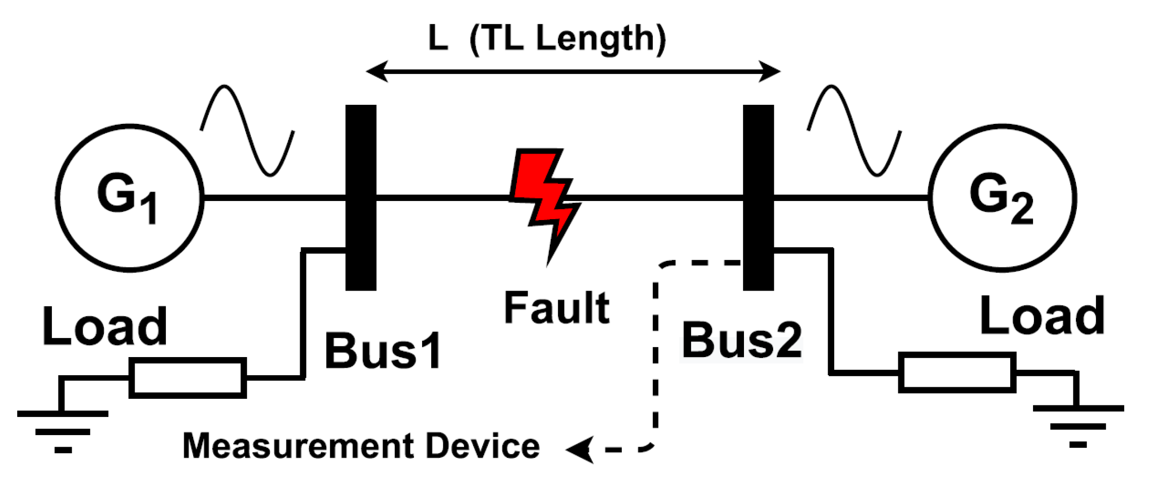
Figure 1 shows the illustrative demonstration of two-terminal transmission networks for transmitting power from generating sources to multiple types of loads.
Different types of techniques used as wavelet-based, genetic algorithm (GA), PMU-based, and multi-information-based techniques are used for the categorization of abnormal conditions on power transfer lines and are not able to provide satisfactory results. Traditionally, fault diagnosis and location in power transmission networks have been performed using rule-based or model-based approaches that require a detailed understanding of the network topology and fault characteristics [4-5]. However, the advent of artificial intelligence approaches is replacing the trade-off methodologies, which are incredibly time-consuming, and their accuracy has limited the complexity of the networks and variability of fault conditions. Tracing abnormal conditions by implementing machine learning and deep learning architectures on power transfer networks is a research area that aims to develop accurate and efficient ML algorithms that can work under faulty conditions more accurately than trade-off planning techniques [6-7].
Figure 2 shows the high-level overview to diagnose faults on transmission lines.
Unfortunately, acquiring labeled data poses significant challenges and time constraints, particularly within power systems where abnormal conditions are infrequent and often unpredictable. To address this issue, recent studies have investigated the potential of utilizing synthetically generated data to enhance the recital of ML architectures. Specifically, generative adversarial networks (GANs) and variational encoders (VAEs) have been utilized to create artificial data that closely aligns with the unique data distribution. [
8]. VAEs are data creation models that can be trained as a low-dimensional representation of the input data and employed to generate new data points. In [
9], the authors proposed a signal spectrum-based machine learning approach by employing diverse ML algorithms to diagnose the hidden patterns of abnormal conditions by predictive maintenance. In [
10], the authors pay attention to diagnosing the faults in electrical machines by employing condition-monitoring techniques for creating datasets. In [
11], the authors proposed a VAE-generated synthetic data-based fault diagnosis method for power transmission lines to augment the limited labeled data and achieve higher accuracy than traditional machine learning algorithms. In [
12], researchers proposed a novel protection scheme for double-circuit transmission lines, aiming to classify shunt faults and accurately localize them through KNN. In [
13], the authors recommended an approach using Variational Autoencoders (VAE) was put forward for fault diagnostics in wind turbines by utilizing synthetic data.
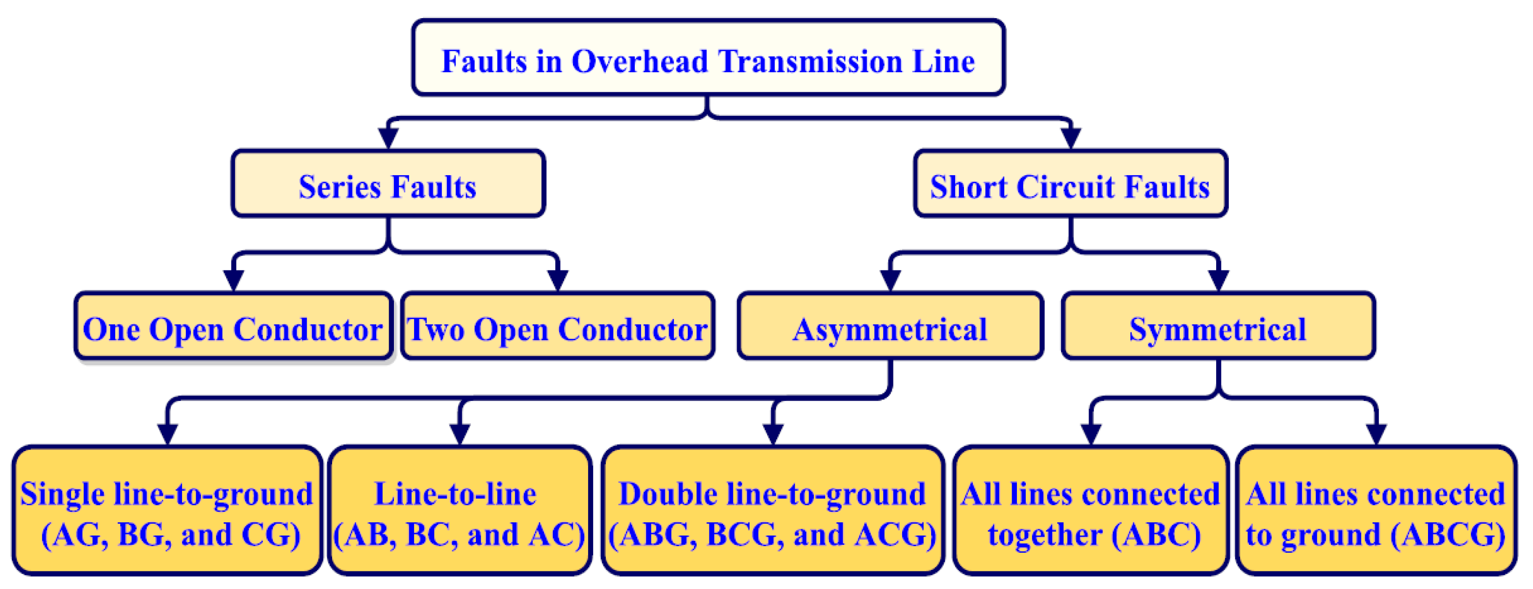
Figure 3 shows the classification for all types of shunt faults that commonly take place on power transmission networks.
Table 1.
The details of standardized approaches employed in this paper are given below:.
Table 1.
The details of standardized approaches employed in this paper are given below:.
| Algorithm |
Type |
Use case |
Pros |
Cons |
| Support vector machines |
Supervised |
Classification
Regression |
Effective handling of outliers through kernel tricks |
Creates problems with noisy & large datasets |
| Decision trees |
Supervised |
Classification
Regression |
Highly interpretable and easy to implement |
Small changes in data creates different tree structures |
| Random forests |
Supervised |
Classification
Regression |
Implement ensemble averaging for predictions |
Less interpretable due to large no. of decision tress |
| K-Nearest neighbors |
Supervised |
Classification
Regression |
Minimum assumptions for data distribution |
Computationally cost and sensitive of K |
1.1. Variational autoencoders
Variational autoencoders (VAEs) are creative models for probabilistic data comprehension. These autoencoders can learn the probability distribution of input data and create new data points that match the training data. VAEs combine auto-encoders and probabilistic models for unsupervised learning tasks like data generation and dimensionality reduction. Image and audio recognition, along with natural language processing and data compression, make extensive use of these techniques. VAEs operate by acquiring a latent representation of the input data, which is a compressed representation capturing the most crucial features. This latent representation facilitates the generation of new data points closely resembling the original training data. [
14]. The key innovation of VAEs is that they use variational inference to learn the latent representation of the data. This involves optimizing an objective function that balances the reconstruction error of the autoencoders with a regularization term that ensures the latent representation follows a desired probability distribution. The regularization term is usually chosen to be a normal distribution, which allows for efficient sampling of the latent space and generation of new data points. The VAE intends to optimize the following loss function:
The reconstruction loss evaluates the variance among the input data, represented as x, and the renovate yield, denoted as x'. On the other hand, the KL divergence loss assesses the distinction between the distribution across the latent representation, z, and a predetermined prior distribution.
1.2. Data synthesis
Data synthesis or data augmentation is a common machine learning method for producing new training data from existing datasets. This strategy introduces variations not in the training data to improve model resilience. Sampling data class feature spaces improve classifier performance. Consequently, this technique aids in achieving better generalization and overall model performance. In domains where data is scarce, pattern recognition tasks can be particularly challenging due to limited variability in the available data, hindering the model's ability to learn effective generalization [
15]. To address this issue in the classification task one can use data augmentation techniques to create additional variations within the existing training data while preserving labels. This can help to amplify the variance within the guidance classes and recover the model’s ability to generalize. It involves merging and integrating data from various sources often using statistical or computational methods to identify patterns, relationships and trends that may not be apparent from individual datasets alone. Data synthesis can be particularly useful in research where it can help to overcome the limitations of individual studies by combining the results of multiple studies to provide a comprehensive understanding of the particular topic.
1.3. Forward feature selection
Feature selection (FS) plays a vital role in supervised learning tasks by identifying pertinent features that exhibit strong correlations with the target variable, while simultaneously removing redundant ones. This crucial process helps reduce computational burdens and improve the accuracy of results. By eliminating redundant features, the selection process ensures a more efficient and effective analysis. In this research, forward feature selection is employed to pick a subset of inputs and eliminate redundant attributes. The process of forward feature selection commences with an initial empty set of features and progressively incorporates the most crucial ones. This is guided by a predetermined criterion, which could involve factors like the strongest correlation with the target variables or the lowest p-values from statistical tests. This process continues until a stopping requirement like max features or model performance is fulfilled. This method iteratively computes the favorable features that exhibit the highest scores thereby avoiding overfitting. The evaluation function used in this study is stratified cross-validation because mostly synthesized generated datasets have imbalanced data and stratified CV can handle the imbalance in the datasets [
16].
3. Proposed Methodology and Contributions
A lot of data is needed to develop good models for many machine-learning applications. Synthetic datasets are too important to generate when real-world data is scarce. Machine learning and deep learning algorithms can create synthetic data from existing datasets to guide ML architectures. The datasets train the ML model for fault classification and transmission line localization. No-missing datasets are ideal. Datasets train machine learning models. Classifying faults requires these ML models. After training the ML model, testing is carried out on the ML model to check the accuracy models.
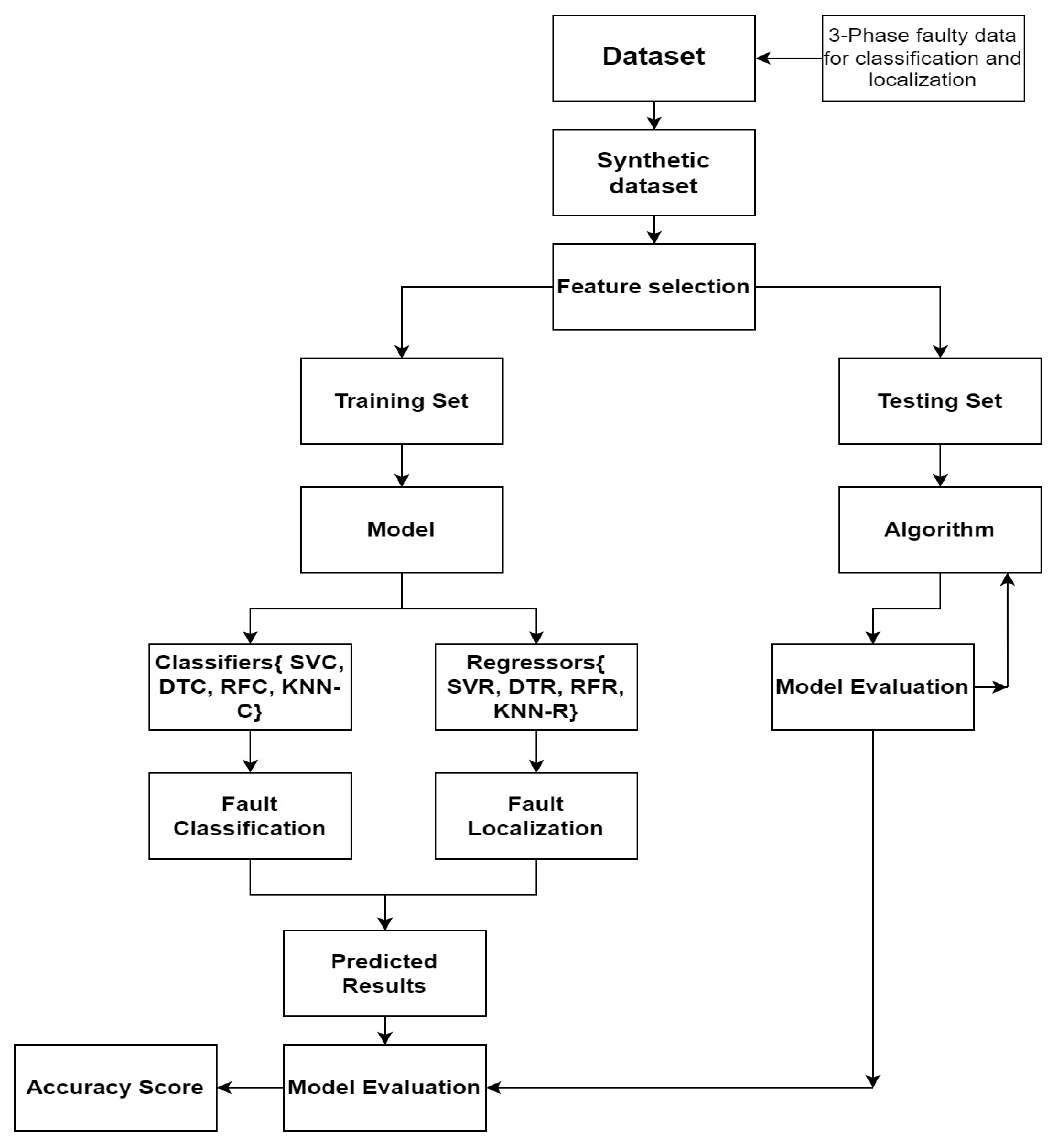
Figure 4 shows the proposed methodology for the classification and regression of abnormal circumstances in transmission-carrying networks. SVMs are useful for fault classification and localization, assisted by supervision to find the hyperplane for separating data point types [
17]. They may considerably improve fault classification and localization processes to find the best hyperplane in n dimensions [18-19]. Define a maximum tree depth to minimize overfitting in decision tree classifiers that employ information gain and Gini index scoring algorithms. The system adjusts depth to balance generalization and training set performance [
23]. Gini index, entropy, and CART determination analyze points [24-25]. Random Forest divides the dataset into training data (the “in bag” data) and validation data (the “out of the bag” data) to detect power system problem characteristics [26-28]. This unpredictability diversifies ensemble trees and improves algorithm performance [29-30]. KNN improves power transmission system fault management by detecting and categorizing defects [
31]. Euclidean, Manhattan, and Mahalanobis distances are used to improve the K-nearest neighbors (KNN) method [32-33]. Approximate KNN approaches use indexing structures like KD-trees and Hash tables to reduce the search space and improve computing performance, especially for big, unbalanced datasets [
34]. This paper has the following attractive contributions.
Introduction of variational autoencoders VAE for the generation of synthetic data for transmission lines fault classification and localization that has ability to improve the classification accuracy than traditional methods.
The technique is cost-effective and practical since it eliminates the requirement for a large volume of labeled real-world data.
Demonstrate the capacity to detect faults in real time and respond quickly, which can reduce the likelihood of power outages and improve grid dependability.
Highlight the system's ability to save time and effort by reducing the frequency of human monitoring and intervention.
Used proposed machine learning architectures with their optimum parameters through tuning for achieving the high accuracy as compared to traditional architectures.
Demonstrate how machine learning applications trained on this improved synthetically generated data can accurately classify power transmission network problems.
4. Description of the experimental setup and data generation
The proposed methodology involves the utilization of experimental platforms encompassing both two-terminal and three-terminal transmission networks. The assessment of these transmission models entails the application of Aspen One-Liner, a productivity-enhancing tool geared toward analyzing and modeling transmission and distribution networks. This software effectively compiles replicated data by simulating diverse transmission network defects under varying operational conditions, facilitating the export of relay testing fault data. During instances of transmission network malfunction, post-fault voltages in all three phases (Va, Vb, and Vc) along with the ground mode are meticulously recorded for a single cycle at each terminal. In pursuit of generating real-time datasets, fault levels are manipulated by introducing alterations in various transmission network fault conditions across multiple locations. This real-time dataset is then employed to enhance the original dataset, resulting in the creation of a synthetic dataset.
Table 5 presents comprehensive data sample information about a range of shunt faults that have occurred on both the two-terminal and three-terminal transmission lines. Applying variational encoders (VAEs) to the list of defects within
Table 2 yields a total of 2183 synthetic samples, further enriching the dataset.
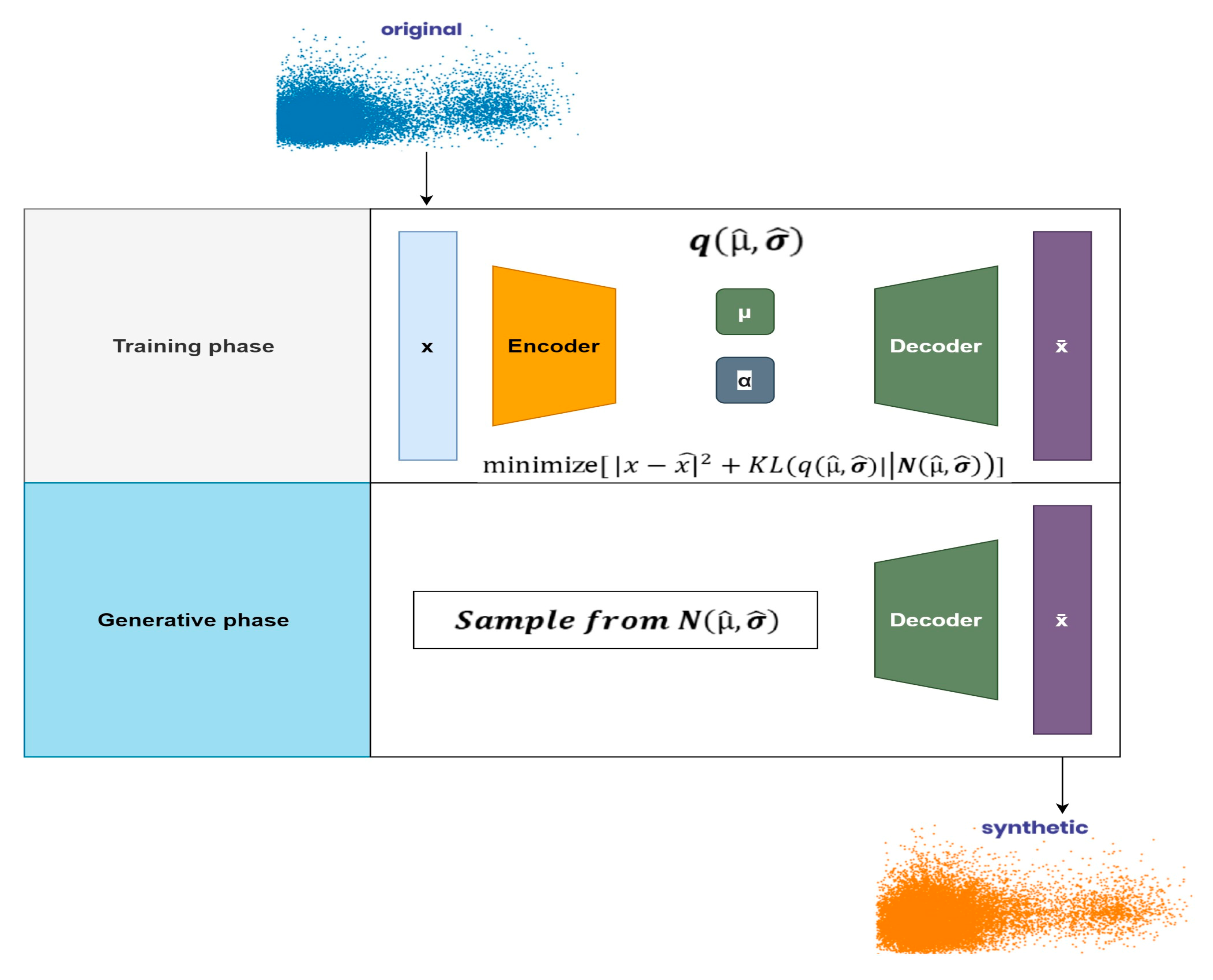
VAEs are talented algorithms that can create synthetic data for double and triple power transmission networks for abnormal conditions classification and localization. This novel method uses Aspen One-liner data samples to construct a new dataset. VAEs, a sort of generative model, may encode input data into a compact latent space and decode it to generate novel data samples that closely match the original data distribution this strategy has shown promise in several applications, including resolving imbalanced class distributions by using synthetic examples [
35]. Generating a synthetic dataset from the original dataset is extremely beneficial in critical situations where the existing dataset is small and imbalanced, and we want to generate some additional data to get better the recital of your ML model. After generating some samples of shunt faults for transmission networks variational encoders VAEs are employed to enlarge this synthetically. Real-time fault recorders are used for recording real-time faulty samples for transmission networks [36-37].
Figure 5.
Proposed Architecture of variational encoder for generation of synthetic data during the training phase and generative phase.
Figure 5.
Proposed Architecture of variational encoder for generation of synthetic data during the training phase and generative phase.
They also duplicate the patterns present in the initial dataset by employing encoder and decoder functions. These functions transform the original dataset into a smaller version, effectively creating an expanded synthetic version. These datasets include information such as phase voltages, location details, and various examples of shunt faults found in transmission networks. This artificially generated data is utilized to teach the ML architectures and assess the effectiveness of the designs. For three-terminal networks only two samples are taken faulty samples for each fault type and similarly, for two-terminal networks one faulty sample are considered as faulty. All types of shunt faults as mentioned in
Table 7 are simulated at each value for both transmission networks. Attributes of training and testing datasets are shown in
Table 3. The fault classification accuracy and localization error of the given dataset by employing machine learning algorithms are 99.13% and < 2% respectively.
4.1. Data splitting
The dataset includes two essential sets: a) the training set, and b) the evaluation set
In the domain of ML algorithms, the process of dividing action datasets into training and testing sets holds great importance. In our suggested approach, the dataset has been partitioned, allocating 70% for training purposes and the remaining 30% for testing. After the algorithm has been trained, the model's effectiveness will be assessed by examining its performance on the testing data.
5. Performance Evaluation and Comparative Analysis
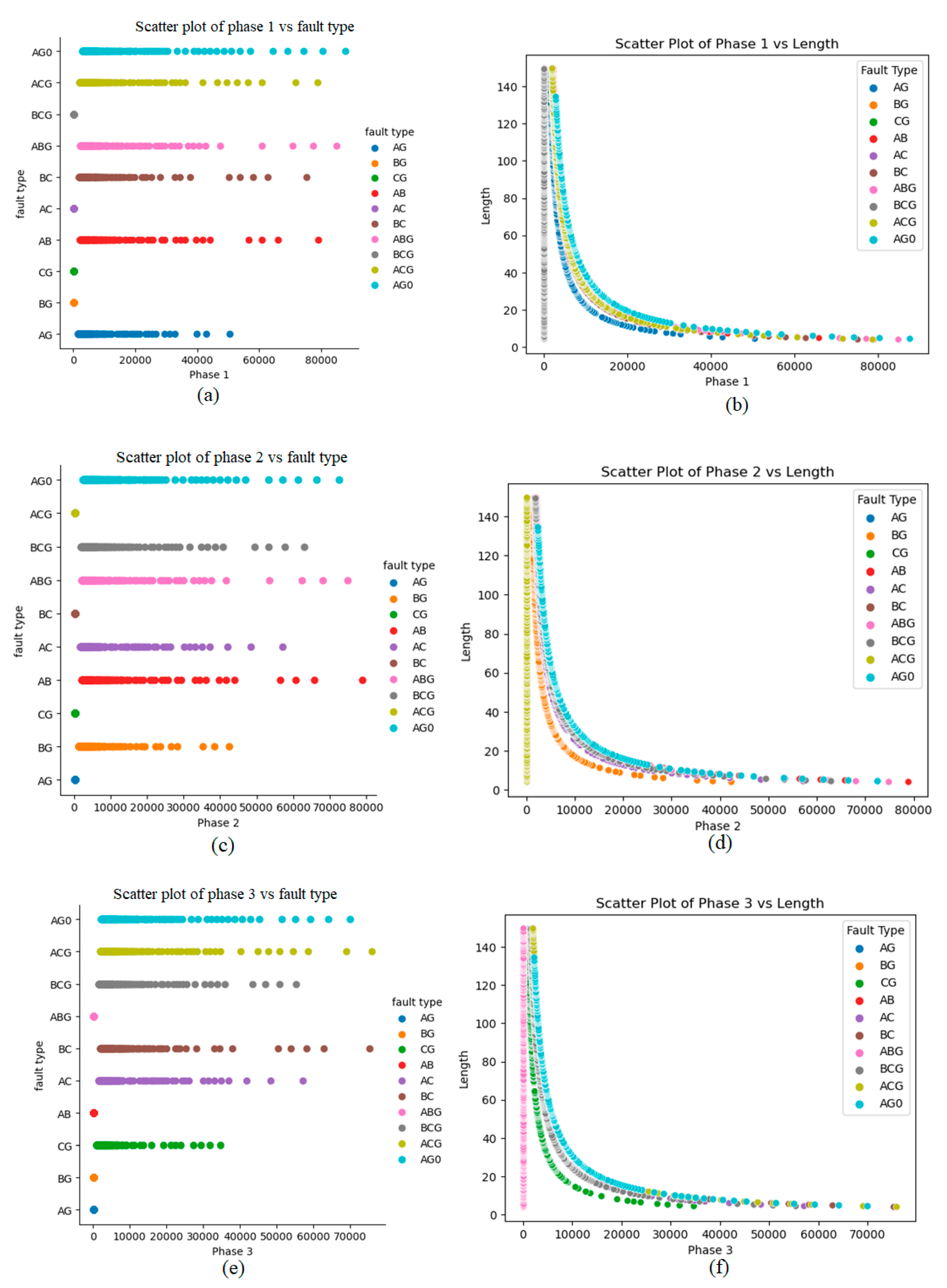
This section aims to provide a concise overview of the synthetic dataset, highlighting its connections to various types of shunt incidents occurring on transmission lines, along with their respective locations. Furthermore, we will introduce a comprehensive set of evaluation metrics that effectively gauge the performance of both the classifier and regressor models. To visually portray the data distribution, we will adopt scatter plots, a technique that presents data points on a two-dimensional graph. This method serves as a robust tool for visualizing relationships and patterns embedded within the dataset. The utilization of scatter plots is intended to enhance the clarity and intuitive understanding of the dataset's complexities, facilitating a deeper exploration of individual interactions and behaviors.
Figure 6 provides the scatter information of every value present in the synthetic generated dataset through VAE,s for classification and localization of faulty points of (a) phase 1, (b) phase 2, and (c) phase 3 respectively.
5.1. Confusion matrixes for predictive modeling of classification algorithms
In this study, we employ a confusion matrix to assess various types of shunt faults, encompassing line-to-ground faults (AG, BG, and CG), line-to-line faults (AB, BC, and AC), double line-to-ground faults (ACG, BCG, and ABG), as well as three-phase faults (ABC-G). Four tentative scenarios are evaluated to measure the performance of the proposed ML algorithms based on accuracy for calculating the ratio of the correctly classified and unclassified abnormal circumstances against the total number of values. The accuracy is calculated as:
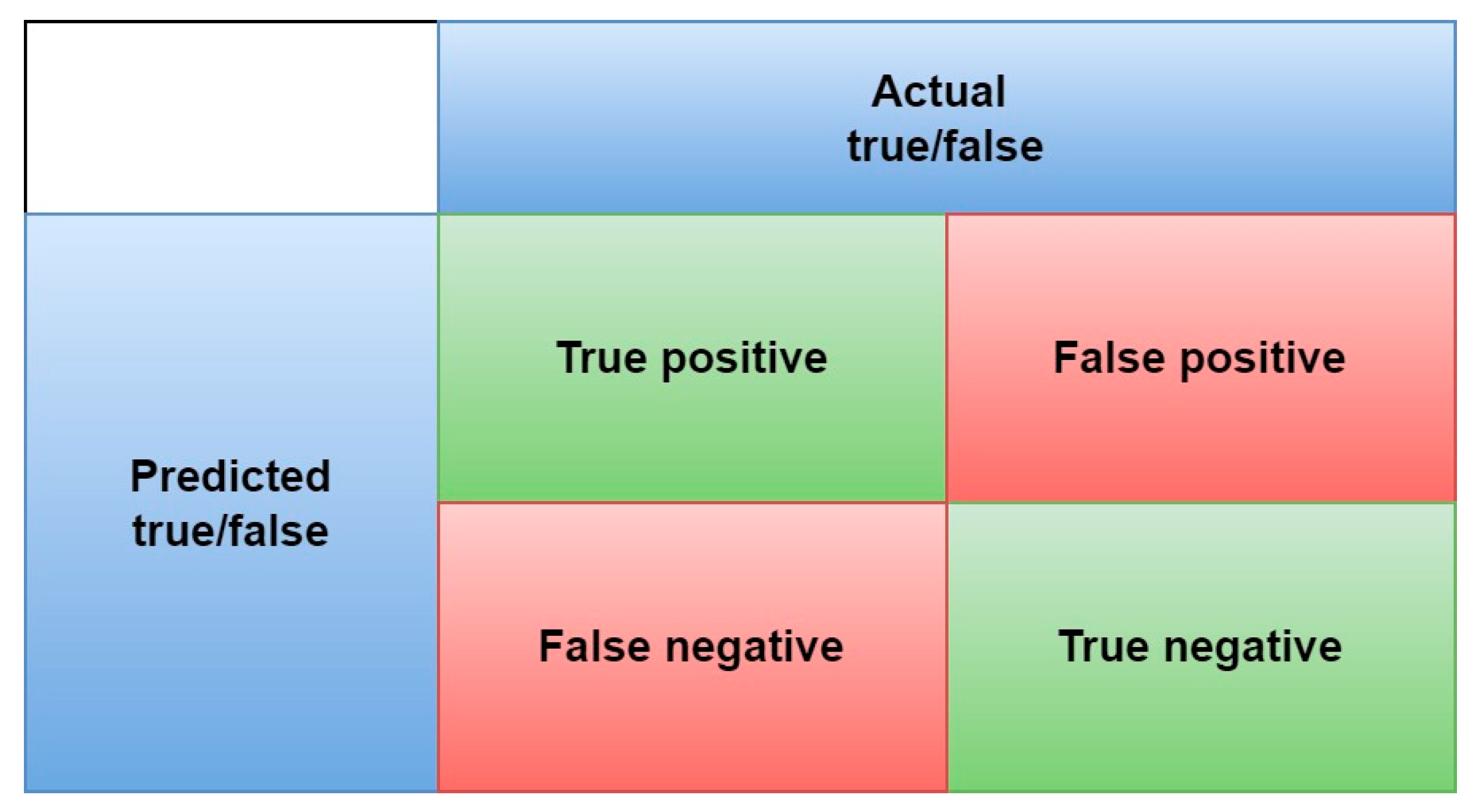
In the context of classification analysis, the acronyms TP (True Positive), TN (True Negative), FP (False Positive), and FN (False Negative) hold significant meaning. These descriptions result from a confusion matrix that presents a counter-process of the predictive performance of a classification model.
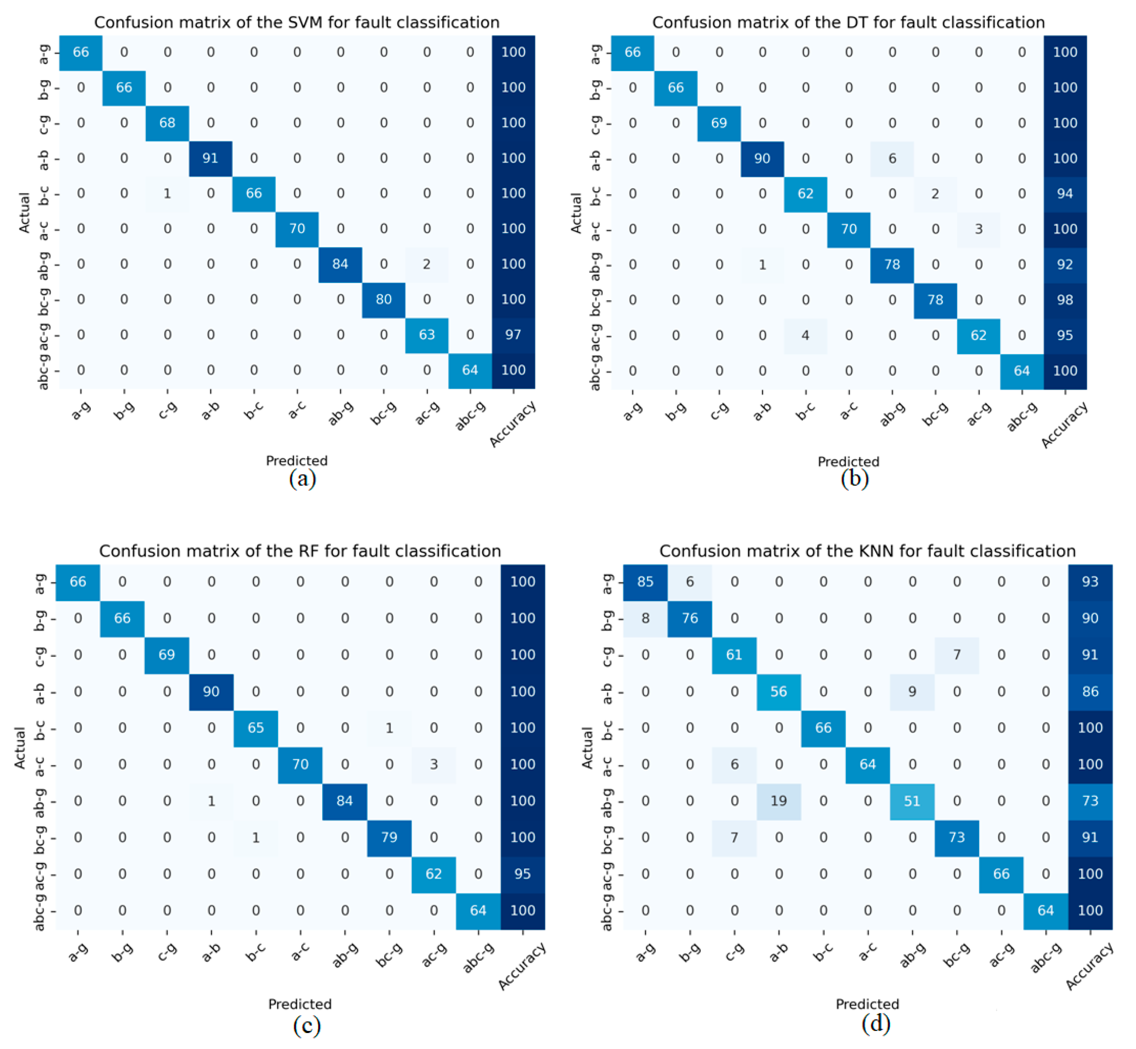
Figure 7, shows the accuracy matrix for diagnosing of predicting outcomes based on proposed architectures for all kinds of shunt faults on power transfer networks.
5.2. Models Hyperparameters Tuning
A hyperparameter research was carried out to find the best settings for RFR and the other models to be compared with. To find the optimal hyperparameters, researchers can choose one of two routes: There are two types of searches: grid searches and random searches. Using a sample of the data, Grid-Search was used to investigate the important parameters for each model and their optimal values. For KNN, we settled on uniform and distance weighting functions, each with different numbers of neighbors. In SVM, both polynomial and radial basis function (RBF) kernels were selected. In addition, we looked at several different values for the regularization parameter C. The lowest number of samples required to divide a node internally in DT was found, and various values were examined to regulate unpredictability inside the tree. Alpha and lambda were chosen as the shape parameters for NB. Alpha represents the Gamma distribution before alpha, while lambda represents the distribution before lambda. To find the appropriate split, the RFR technique used two maximum feature methods, sqrt, and log2, to calculate the number of characteristics to evaluate.
Table 3 shows Grid-Search results for several models. The best parameters for each model are highlighted.
Table 4, shows the optimal hyperparameter through a hyperparameter search for appropriate values to enhance the accuracy of the training model of SVM for the proposed methodology.
To calculate the classification truth of shunt faults, the dataset is separated into training and testing subsets, with 70% of the data allocated for training and the remaining 30% for testing. The confusion matrix offers valuable insights into classification precision, where the diagonal elements signify accurately predicted cases, and the off-diagonal values represent misclassifications.
Figure 8 illustrates the Visual representations of the confusion matrices for (a) SVM, (b) DT, (c) RF, and (d) KNN to diagnose shunt faults on power transfer networks.
The confusion matrix is employed to visualize the numeric test results, including true positives, true negatives, false positives, and false negatives, highlighting the effectiveness of the machine learning classifier [
39]. In this matrix, the diagonal values represent accurately classified instances, while the non-diagonal values correspond to unclassified instances in the fault classification task for power transmission lines.
Table 5 presents the fault classification results for the proposed machine learning algorithms, namely SVM, DT, RF, and KNN, as utilized in this study. It also demonstrates that the classification results for shunt defects that occurred on power transmission lines using the machine learning algorithms proposed in this article are extremely high accuracy up to (99.50%).
Table 5.
Testing results of fault classification for different machine learning algorithms.
Table 5.
Testing results of fault classification for different machine learning algorithms.
| Machine learning model |
Fault types |
No. of test data samples |
Accurately classified samples |
Misclassified samples |
Accuracy
% |
| |
LG(a-g,b-g,c-g) |
200 |
199 |
1 |
99.95 |
| SVM |
LL(a-b,b-c,c-a) |
227 |
227 |
0 |
100 |
| |
LL-G(ab-g,bc-g,ac-g) |
227 |
225 |
2 |
99.11 |
| |
LLL(abc) |
64 |
64 |
0 |
100 |
| |
LG (a-g,b-g,c-g) |
201 |
201 |
0 |
100 |
| DT |
LL (a-b,b-c,c-a) |
222 |
217 |
5 |
97.74 |
| |
LL-G (ab-g,bc-g,ac-g) |
218 |
207 |
11 |
95.95 |
| |
LLL (abc) |
64 |
64 |
0 |
100 |
| |
LG (a-g,b-g,c-g) |
201 |
201 |
0 |
100 |
| RF |
LL (a-b,b-c,c-a) |
226 |
224 |
2 |
99.11 |
| |
LL-G (ab-g,bc-g,ac-g) |
225 |
221 |
4 |
98.22 |
| |
LLL (abc) |
64 |
64 |
0 |
100 |
| |
LG (a-g,b-g,c-g) |
242 |
222 |
20 |
91.73 |
| KNN |
LL (a-b,b-c,c-a) |
195 |
186 |
9 |
95.38 |
| |
LL-G (ab-g,bc-g,ac-g) |
216 |
190 |
26 |
87.96 |
| |
LLL (abc) |
64 |
64 |
0 |
100 |
5.3. Parameters for Evaluating the Performance of Classification Models
There are various methods to evaluate the efficiency of classification architectures, which rely on the attributes of the test dataset. These methods include well-known measures such as accuracy, precision, recall, and F1 score, derived from the confusion matrix analysis [
40]. These evaluation metrics are computed based on the elements of the confusion matrix plot, tailored to the specific domain of the problem, and offer a thorough understanding of the analysis. The outcomes of these assessment metrics are demonstrated in
Table 6, presenting the results of the classification models in terms of their performance measures.
5.4. Receiver Operating Characteristic (ROC) Analysis for proposed architectures
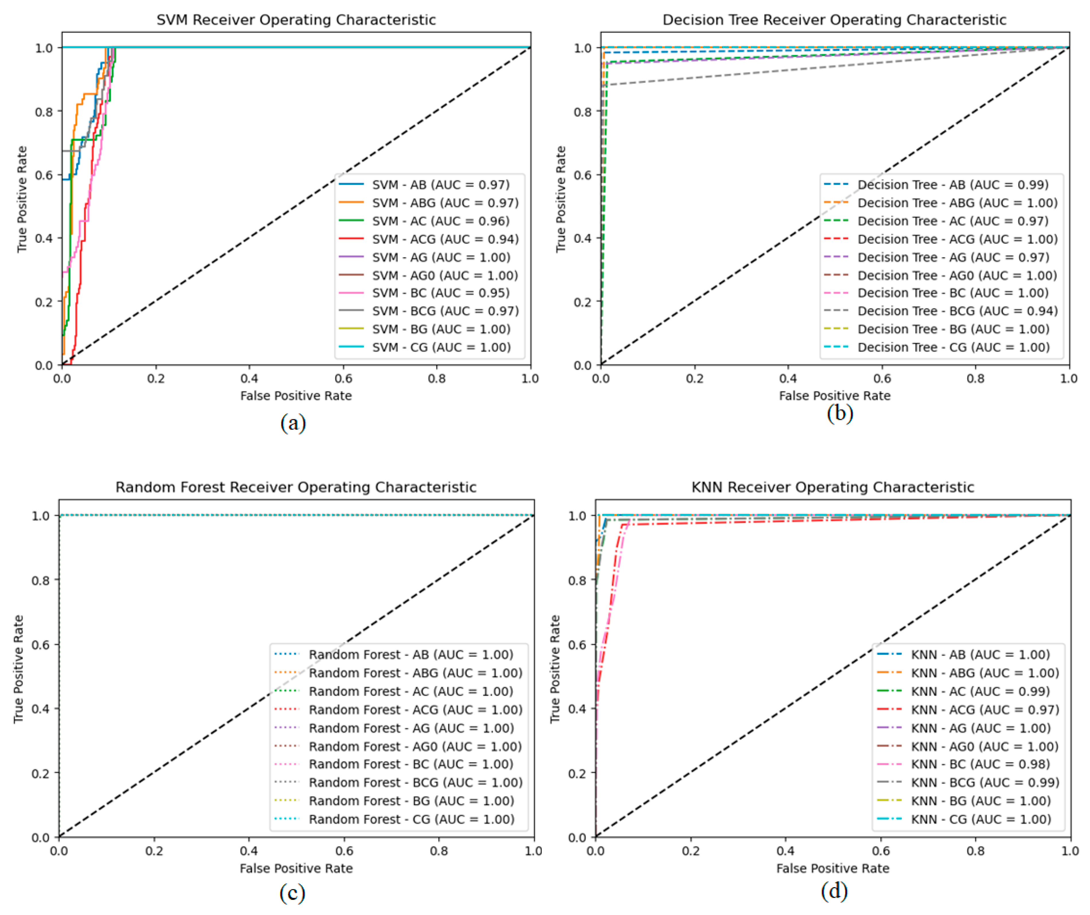
ROC curves assessed classification models and shows the model's classification efficiency when thresholds change through ability to distinguish classes by balancing sensitivity and specificity. Four classifiers—SVM, Decision Tree, Random Forest, and KNN—were examined. We predicted class membership probability for the test dataset after training each classifier. These predicted probabilities generated ROC curves. FPR and TPR are on x and y. Random guessing ROC curve is a dashed black diagonal line. Classifiers hope curves over this diagonal outperform random chance. Starting with the SVM classifier (solid lines), we get fault-type-specific ROC curves with AUC values. AUC improves class separation. Dashed Decision Tree classifier ROC curves capture complex decision boundaries. The Random Forest classifier (dotted lines) uses many decision trees to smooth fault-type curves. ROC curves for the neighborhood-based k-nearest neighbor (KNN) classifier (dot lines). Dataset and neighbor count affect KNN performance. ROC curves reveal each classifier's strengths and weaknesses. This helps us find fault-tolerant and multi-class models. We prioritize ROC curves and AUC values for classification model evaluation. These metrics help select a problem domain's best classifier by assessing a model's class discrimination.
Figure 9; shows the roc curve for SVM, DT, RF, and KNN to show the accuracies of classification results on the power transmission lines.
5.5. Fault localization results
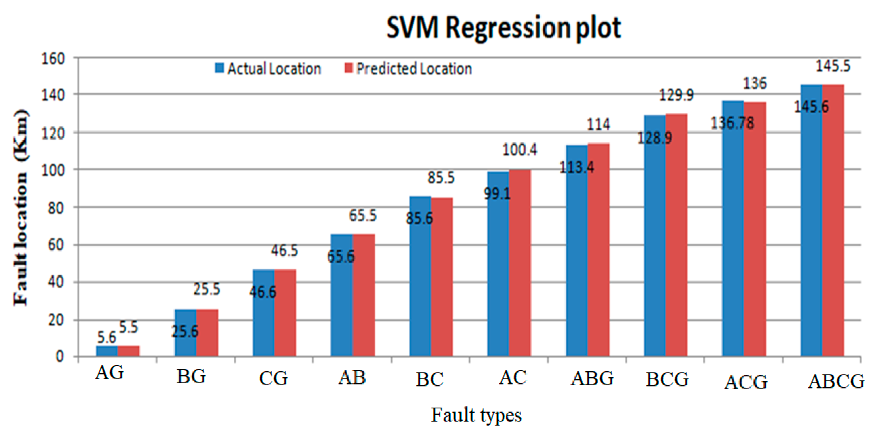
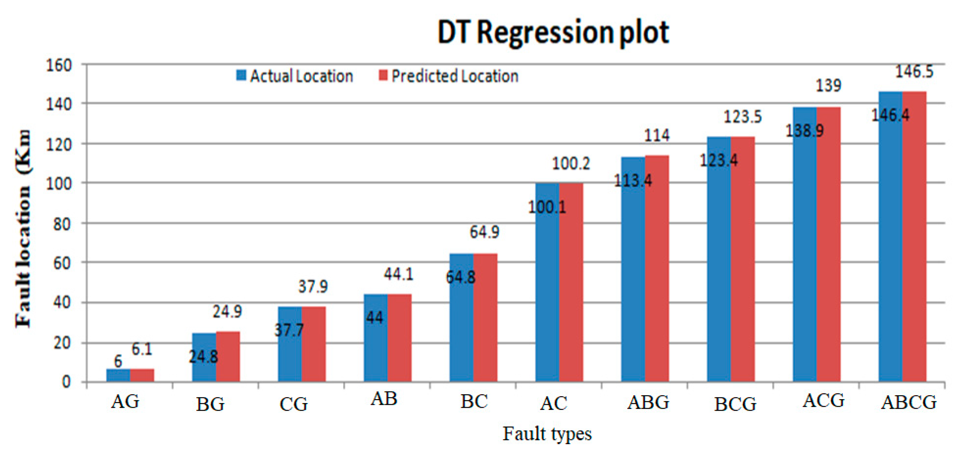
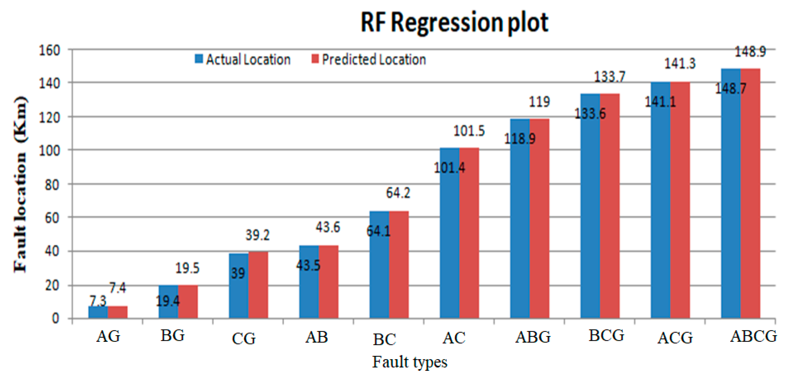
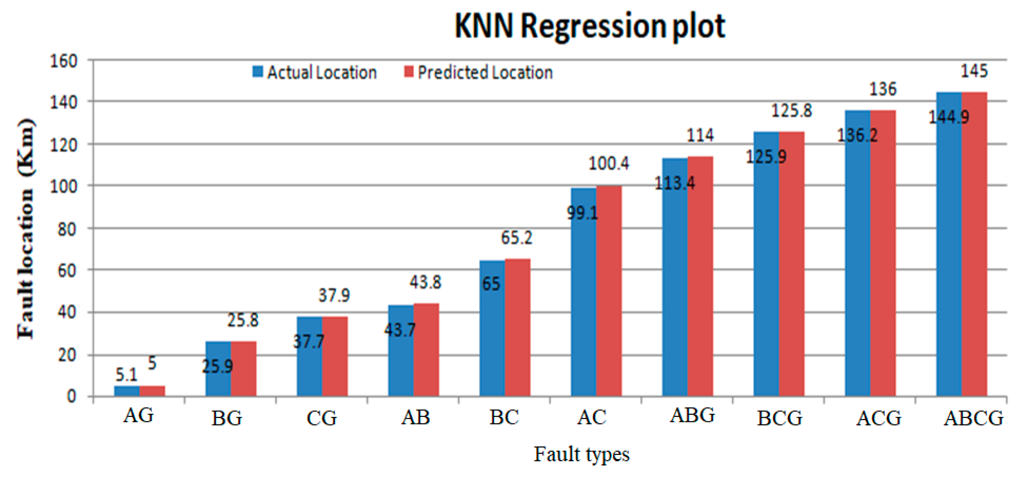
Once the fault type has been identified through the proposed classifier architecture, the precise prediction of shunt fault locations within transmission networks is achieved using regression models. The primary objective of these regression models is to establish a functional mapping between the input features (independent variables) and the target variable (a continuous value). Furthermore, regression serves as a means to uncover the intricate relationship between continuous input variables and their corresponding output variables. In the capacity of a regressor, a selection of diverse machine learning algorithms comes into play to pinpoint power line faults. The process involves conducting regression computations for unforeseen data instances, accounting for both the proximity and distance of the ends under observation. The regression outcomes are delineated in Figures 10, 11, 12, and 13, illustrating a comparative analysis between the actual fault locations and those predicted by the proposed machine learning algorithms (SVM, DT, RF, and KNN).
Figure 10.
Actual and predicted fault locations using support vector machine (SVM).
Figure 10.
Actual and predicted fault locations using support vector machine (SVM).
Figure 11.
Actual and predicted fault locations using decision trees (DT).
Figure 11.
Actual and predicted fault locations using decision trees (DT).
Figure 12.
Actual and predicted fault locations using random forest (RF).
Figure 12.
Actual and predicted fault locations using random forest (RF).
Figure 13.
Actual and predicted fault locations using K-nearest neighbors (KNN).
Figure 13.
Actual and predicted fault locations using K-nearest neighbors (KNN).
The regression results for the proposed machine-learning algorithms are shown in
Table 6. The actual values are shown by a blue line as mentioned in the regression graph and the regression line is shown by the red dotted line. So, the regression line is linear and the accuracy of the regression system predicted good results. The regression fit line for fault localization on the power transmission networks is shown in
Table 6. The term absolute error is used to evaluate the regression results on the power lines. The absolute error gives the results of the actual length on which the fault occurred and predicted results, which are predicted by machine learning models. In absolute error y-predicted is the value predicted by the machine learning model and y-true is the true fault distance. The absolute error is given as
Table 7 presents the outcomes of the regression model for both real and predicted fault localization values. It also illustrates the extent of error experienced in power transfer lines due to the implementation of the suggested approach.
Table 7.
Table for true and predicted values of fault localization and amount of error.
Table 7.
Table for true and predicted values of fault localization and amount of error.
| Machine learning model |
True fault distance |
Predicted fault distance |
% of Error |
| |
116.9 |
115.6 |
1.3 |
| SVM |
104.4 |
103.7 |
0.63 |
| |
52.4 |
49.5 |
2.80 |
| |
115.1 |
113.8 |
1.36 |
| |
21.6 |
21.2 |
0.4 |
| DT |
114.2 |
112.8 |
1.4 |
| |
74.4 |
72.3 |
2.1 |
| |
50.0 |
49.2 |
0.8 |
| |
61.2 |
59.7 |
1.5 |
| RF |
48.1 |
47.6 |
0.58 |
| |
103.3 |
102.4 |
0.92 |
| |
146.4 |
144.3 |
2.09 |
| |
115.6 |
114.8 |
0.8 |
| KNN |
104.4 |
103.9 |
0.48 |
| |
112.8 |
110.2 |
2.6 |
| |
21.2 |
20.2 |
0.99 |
6. Conclusions
This study demonstrates the different machine learning algorithms for the recognition of all types of shunt faults on transmission lines and their location tracing based on synthetic data instead of using traditional trade-off planning. Transmission networks are the most critical part of the power transfer system and are used to transfer power from one end to far ends. Different protecting relaying systems are installed on the grid/substation for the sensitive operations of transients which mostly occur on the power system. When abnormal conditions occur, then it will be necessary to remove the faults within no time and restore the power to end-users. The collection of real data for making datasets is the major problem in implementing and training models. This study is based on the analysis of data obtained from simulations of transmission networks using aspen one-liner, which is further expanded by employing variational encoders to enlarge it synthetically. Machine learning algorithms are the best solution for complex networks. These algorithms are easy to implement, and the best performance results can be obtained, restoring the power supply for a safe and reliable country's energy system. The proposed methodology is simple to implement for the existing protection system. Machine learning models are trained by datasets and feature selection methods. In the classification process, the model is trained to classify the shunt faults, which mostly occur in the power system. Support vector machines, decision trees, random forests, and KNN models are used for classification and regression. All the classifiers provide admirable results for the classification and localization of faults on transmission networks. This research work also highlights the importance of data quantity, and increasing the amount of data synthetically for training improves the accuracy of architectures they also emphasize the need for accurate fault data labeling and feature selection to achieve optimal results.
Author Contributions
“Conceptualization, M.A.K. and B.A.; methodology, M.A.K.; validation, B.A., T.V..; formal analysis, A.K.; investigation, M.A.K.; resources, T.V., R.P., and V.K.H; data curation, M.A.K. and B.A..; writing—original draft preparation, M.A.K; writing—review and editing, M.A.K., B.A.; visualization, T.V.; supervision, B.A., T.V., R.P. and V.K.H; project administration, T.V.; funding acquisition, T.V., R.P., V.K.H.; All authors have read and agreed to the published version of the manuscript.”
Data Availability Statement
Not applicable.
Acknowledgments
The “Industrial Internet methods for electrical energy conversion systems monitoring and diagnostics” benefits from a 993000 € grant from Iceland, Liechtenstein and Norway through the EEA Grants. The aim of the project is to provide the research in field of energy conversion systems and to develop artificial intelligence and virtual emulator-based prognostic and diagnostic methodologies for these systems. Project contract with the Research Council of Lithuania (LMTLT) No is S-BMT-21-5 (LT08-2-LMT-K-01-040).
Conflicts of Interest
The authors declare no conflict of interest.
References
- Dinsdale, Nicholas J., Peter R. Wiecha, Matthew Delaney, Jamie Reynolds, Martin Ebert, IoannisZeimpekis, David J. Thomson et al. "Deep learning enabled design of complex transmission matrices for universal optical components." ACS photonics 8, no. 1 (2021): 283-295. [CrossRef]
- Vaish, Rachna, U. D. Dwivedi, Saurabh Tewari, and Saurabh Mani Tripathi. "Machine learning applications in power system fault diagnosis: Research advancements and perspectives." Engineering Applications of Artificial Intelligence 106 (2021): 104504. [CrossRef]
- Kothari, DwarkadasPralhaddas. "Power system optimization." In 2012 2nd National conference on computational intelligence and signal processing (CISP), pp. 18-21. IEEE, 2012.
- Raja, Hadi Ashraf, Karolina Kudelina, Bilal Asad, Toomas Vaimann, Ants Kallaste, Anton Rassõlkin, and Huynh Van Khang. "Signal Spectrum-Based Machine Learning Approach for Fault Prediction and Maintenance of Electrical Machines." Energies 15, no. 24 (2022): 9507. [CrossRef]
- Raja, Hadi Ashraf, Bilal Asad, Toomas Vaimann, Ants Kallaste, Anton Rassõlkin, and Anouar Belahcen. "Custom Simplified Machine Learning Algorithms for Fault Diagnosis in Electrical Machines." In 2022 International Conference on Diagnostics in Electrical Engineering (Diagnostika), pp. 1-4. IEEE, 2022. [CrossRef]
- Vaimann, Toomas, Anton Rassõlkin, Ants Kallaste, Raimondas Pomarnacki, and Anouar Belahcen. "Artificial intelligence in monitoring and diagnostics of electrical energy conversion systems." In 2020 27th International Workshop on Electric Drives: MPEI Department of Electric Drives 90th Anniversary (IWED), pp. 1-4. IEEE, 2020.
- Tîrnovan, Radu-Adrian, and Maria Cristea. "Advanced techniques for fault detection and classification in electrical power transmission systems: An overview." In 2019 8th International Conference on Modern Power Systems (MPS), pp. 1-10. IEEE, 2019. [CrossRef]
- Zhang, T. , Xia, P., & Lu, F. (2021). 3D reconstruction of digital cores based on a model using generative adversarial networks and variational auto-encoders. Journal of Petroleum Science and Engineering, 207, 109151. [CrossRef]
- Stetco, A., Dinmohammadi, F., Zhao, X., Robu, V., Flynn, D., Barnes, M., ... & Nenadic, G. (2019). Machine learning methods for wind turbine condition monitoring: A review. Renewable energy, 133, 620-635. [CrossRef]
- Kudelina, K., Asad, B., Vaimann, T., Rassõlkin, A., Kallaste, A., & Khang, H. V. (2021). Methods of condition monitoring and fault detection for electrical machines. Energies, 14(22), 7459. [CrossRef]
- Lu, S., Tang, X., Zhu, Y., & She, J. (2021, June). A cloud-edge collaborative intelligent fault diagnosis method based on LSTM-VAE hybrid model. In 2021 8th IEEE International Conference on Cyber Security and Cloud Computing (CSCloud)/2021 7th IEEE International Conference on Edge Computing and Scalable Cloud (EdgeCom) (pp. 207-212). IEEE.
- Swetapadma, A., Mishra, P., Yadav, A., & Abdelaziz, A. Y. (2017). A non-unit protection scheme for double circuit series capacitor compensated transmission lines. Electric Power Systems Research, 148, 311-325. [CrossRef]
- Zhang, T., Chen, J., Li, F., Zhang, K., Lv, H., He, S., & Xu, E. (2022). Intelligent fault diagnosis of machines with small & imbalanced data: A state-of-the-art review and possible extensions. ISA transactions, 119, 152-171. [CrossRef]
- Utkin, L., Drobintsev, P., Kovalev, M., & Konstantinov, A. (2021, January). Combining an autoencoder and a variational autoencoder for explaining the machine learning model predictions. In 2021 28th Conference of Open Innovations Association (FRUCT) (pp. 489-494). IEEE. [CrossRef]
- Evans, D. (2002). Systematic reviews of interpretive research: interpretive data synthesis of processed data. Australian Journal of Advanced Nursing, The, 20(2).
- Meyer, H., Reudenbach, C., Hengl, T., Katurji, M., & Nauss, T. (2018). Improving performance of spatio-temporal machine learning models using forward feature selection and target-oriented validation. Environmental Modelling & Software, 101, 1-9. [CrossRef]
- Kouziokas, Georgios N. "SVM kernel based on particle swarm optimized vector and Bayesian optimized SVM in atmospheric particulate matter forecasting." Applied Soft Computing 93 (2020): 106410. [CrossRef]
- Parisi, Luca. "m-arcsinh: An Efficient and Reliable Function for SVM and MLP in scikit-learn." arXiv preprint arXiv:2009.07530 (2020). arXiv:2009.07530 (2020).
- Ekici, S. (2012). Support Vector Machines for classification and locating faults on transmission lines. Applied soft computing, 12(6), 1650-1658. [CrossRef]
- Johnson, J. M., & Yadav, A. (2017). Complete protection scheme for fault detection, classification and location estimation in HVDC transmission lines using support vector machines. IET Science, Measurement & Technology, 11(3), 279-287. [CrossRef]
- Fei, C., & Qin, J. (2021). Fault location after fault classification in transmission line using voltage amplitudes and support vector machine. Russian Electrical Engineering, 92(2), 112-121. [CrossRef]
- Quinlan, J. R. (1990). Decision trees and decision-making. IEEE Transactions on Systems, Man, and Cybernetics, 20(2), 339-346. [CrossRef]
- Daniya, T., M. Geetha, and K. Suresh Kumar. "Classification and regression trees with gini index." Advances in Mathematics Scientific Journal 9, no. 10 (2020): 1857-8438. [CrossRef]
- Chen, K., Huang, C., & He, J. (2016). Fault detection, classification and location for transmission lines and distribution systems: a review on the methods. High voltage, 1(1), 25-33. [CrossRef]
- Chen, Y. Q., Fink, O., & Sansavini, G. (2017). Combined fault location and classification for power transmission lines fault diagnosis with integrated feature extraction. IEEE Transactions on Industrial Electronics, 65(1), 561-569. [CrossRef]
- Han, Sunwoo, Brian D. Williamson, and Youyi Fong. "Improving random forest predictions in small datasets from two-phase sampling designs." BMC medical informatics and decision making 21, no. 1 (2021): 1-9. [CrossRef]
- Zhu, Yongli, and Hua Peng. "Multiple Random Forests Based Intelligent Location of Single-Phase Grounding Fault in Power Lines of DFIG-Based Wind Farm." Journal of Modern Power Systems and Clean Energy (2022). [CrossRef]
- Chakraborty, D. , Sur, U., & Banerjee, P. K. (2019, November). Random forest based fault classification technique for active power system networks. In 2019 IEEE International WIE Conference on Electrical and Computer Engineering (WIECON-ECE) (pp. 1-4). IEEE.
- Chen, K. , Huang, C., & He, J. (2016). Fault detection, classification and location for transmission lines and distribution systems: a review on the methods. High voltage, 1(1), 25-33. [CrossRef]
- Zhu, Y. , & Peng, H. (2022). Multiple Random Forests Based Intelligent Location of Single-phase Grounding Fault in Power Lines of DFIG-based Wind Farm. Journal of Modern Power Systems and Clean Energy, 10(5), 1152-1163. [CrossRef]
- Gangwar, Amit Kumar, Om Prakash Mahela, Bhuvnesh Rathore, Baseem Khan, Hassan HaesAlhelou, and PierluigiSiano. "A Novel k-Means Clustering and Weighted k-NN-Regression-Based Fast Transmission Line Protection." IEEE Transactions on Industrial Informatics 17, no. 9 (2020): 6034-6043. [CrossRef]
- Haq, Ejaz Ul, Huang Jianjun, Kang Li, Fiaz Ahmad, David Banjerdpongchai, and Tijiang Zhang. "Improved performance of detection and classification of 3-phase transmission line faults based on discrete wavelet transform and double-channel extreme learning machine." Electrical Engineering 103, no. 2 (2021): 953-963. [CrossRef]
- Dasgupta, A. , Debnath, S., & Das, A. (2015). Transmission line fault detection and classification using cross-correlation and k-nearest neighbor. International Journal of Knowledge-based and Intelligent Engineering Systems, 19(3), 183-189. [CrossRef]
- Gangwar, A. K. , Mahela, O. P., Rathore, B., Khan, B., Alhelou, H. H., & Siano, P. (2020). A Novel $ k $-Means Clustering and Weighted $ k $-NN-Regression-Based Fast Transmission Line Protection. IEEE Transactions on Industrial Informatics, 17(9), 6034-6043. [CrossRef]
- Wan, Z. , Zhang, Y., & He, H. (2017, November). Variational autoencoder based synthetic data generation for imbalanced learning. In 2017 IEEE symposium series on computational intelligence (SSCI) (pp. 1-7). IEEE. [CrossRef]
- Farhadyar, K., Bonofiglio, F., Zoeller, D., & Binder, H. (2021). Adapting deep generative approaches for getting synthetic data with realistic marginal distributions. arXiv preprint arXiv:2105.06907.
- Greco, G. , Guzzo, A., & Nardiello, G. (2020, September). FD-VAE: A feature driven VAE architecture for flexible synthetic data generation. In Database and Expert Systems Applications: 31st International Conference, DEXA 2020, Bratislava, Slovakia, September 14–17, 2020, Proceedings, Part I (pp. 188-197). Cham: Springer International Publishing. [CrossRef]
- Makhtar, M., Neagu, D. C., & Ridley, M. J. (2011). Binary classification models comparison: On the similarity of datasets and confusion matrix for predictive toxicology applications. In Information Technology in Bio-and Medical Informatics: Second International Conference, ITBAM 2011, Toulouse, France, August 31-September 1, 2011. Proceedings 2 (pp. 108-122). Springer Berlin Heidelberg. [CrossRef]
- Sun, T., Li, H., Wu, K., Chen, F., Zhu, Z., & Hu, Z. (2020). Data-driven predictive modelling of mineral prospectivity using machine learning and deep learning methods: a case study from southern Jiangxi Province, China. Minerals, 10(2), 102. [CrossRef]
- Yacouby, R., & Axman, D. (2020, November). Probabilistic extension of precision, recall, and f1 score for more thorough evaluation of classification models. In Proceedings of the first workshop on evaluation and comparison of NLP systems (pp. 79-91).
|
Disclaimer/Publisher’s Note: The statements, opinions and data contained in all publications are solely those of the individual author(s) and contributor(s) and not of MDPI and/or the editor(s). MDPI and/or the editor(s) disclaim responsibility for any injury to people or property resulting from any ideas, methods, instructions or products referred to in the content. |
© 2023 by the authors. Licensee MDPI, Basel, Switzerland. This article is an open access article distributed under the terms and conditions of the Creative Commons Attribution (CC BY) license (http://creativecommons.org/licenses/by/4.0/).
