1. Introduction

2. Materials and Methods

2.1. Site Discription

The study area is located in the region of Naama in southwest Algeria. Naama covers an area of 27,950 km2 and has a population of around 200,000 inhabitants. The climate is arid, characterized by hot, dry summers and mild, rainy winters.

The terrain is relatively flat, situated on an elevated plateau at an average altitude of 800 meters above sea level. The landscape consists of sparse grasslands and desert areas with some low hills and rocky outcrops. Vegetation cover is very low, dominated by scrubland and drought-resistant plants.

Naama has a desert climate, classified as BWh in the Köppen climate classification system. It has long, extremely hot summers and short, warm winters. The average annual temperature is 21.2${}^{\circ }$C. July is the hottest month with average highs of 41.4${}^{\circ }$C. January is the coldest month with average lows of 3.8${}^{\circ }$C.

Rainfall is scarce, averaging just 130 mm per year. Most precipitation falls in the winter months from November to March. The rainy season typically sees brief, intense storms rather than steady rainfall. Summers are completely dry. The low humidity and high solar radiation result in very high rates of evaporation.

Winds are predominantly from the north and west. The area experiences frequent sandstorms and dust storms, especially during the spring. Average wind speeds are highest in June at around 19 km/h. Wind patterns display significant diurnal variations, with calmer winds during mornings and stronger gusts in the afternoons and evenings [6,7] .

Naama has an extremely arid desert climate with hot summers, mild winters, very low rainfall, and strong afternoon/evening winds. The area has high solar energy potential but lacks electricity infrastructure and suffers from power shortages. Developing renewable energy projects can help meet local energy demand in this remote region [6,7].

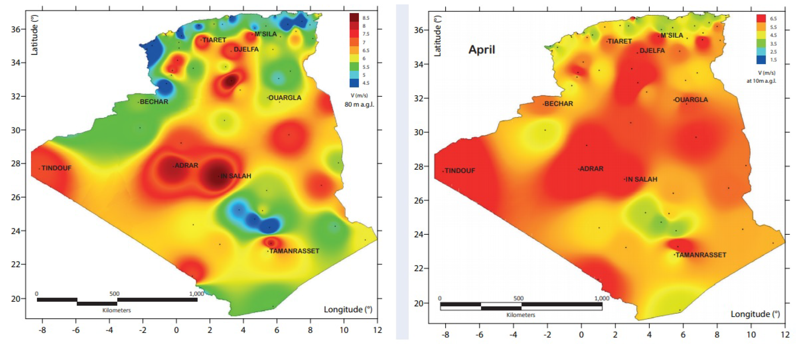
Figure 1. Wind Resources of Algeria: Distribution of the mean wind speed (m/s) across the Algerian territory at 80 m height (left figure) and at 10 m height (right figure)

Figure 1. Wind Resources of Algeria: Distribution of the mean wind speed (m/s) across the Algerian territory at 80 m height (left figure) and at 10 m height (right figure)

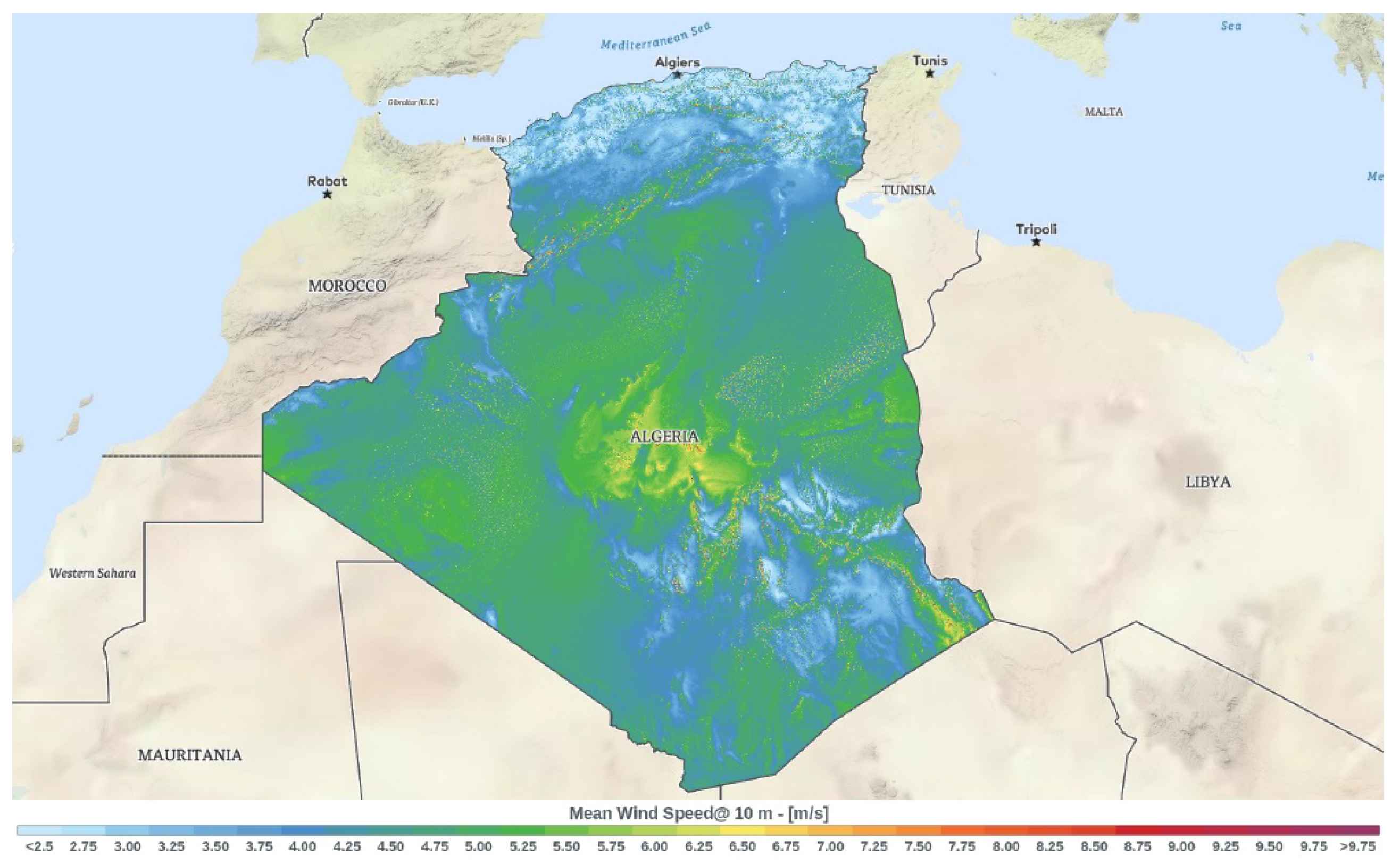
Figure 2. Map of Algeria’s wind resources at 10 m height

Figure 2. Map of Algeria’s wind resources at 10 m height

Figure 3. Aerial photo of the site of the Namaa university center

Figure 3. Aerial photo of the site of the Namaa university center

2.2. Exploratory Wind Data Analysis

The wind resource assessment utilized historical wind speed data from 2012-2022 collected in Naama, Algeria [8,9] . Wind measurements were obtained from a meteorological instrument installed in university center of Naama city. Cup anemometers and wind vanes at heights of 10 m, 30 m, and 50 m logged wind speeds and directions at 1 Hz frequency [10] . The raw data was averaged over 10-minute intervals. Quality control procedures were implemented to filter the data. Limits checks identified unphysical values exceeding threshold bounds which were discarded. Sensor malfunctions and icing events were screened through manual inspection and comparison between heights. Gaps up to 2 hours were filled by linear interpolation. The filtered 10-year Naa ma dataset provided the basis for subsequent wind distribution modeling [9] .

The validated 10-year 10-minute mean wind speed data was analyzed graphically and statistically to assess the general characteristics [8] . Time series plots over different time scales depicted the seasonal and diurnal variability.

The mean, standard deviation, minimum, maximum, median, mode, skewness, and kurtosis quantified the distribution properties. Quantile-quantile plots relative to common theoretical distributions evaluated distribution fit. The exploratory analysis revealed strong Weibull characteristics, with unimodal distribution and positive skewness indicating higher frequency of lower wind speeds [8,10] . The 10-minute mean speeds were aggregated to hourly and monthly resolutions for subsequent distribution modeling [8] .

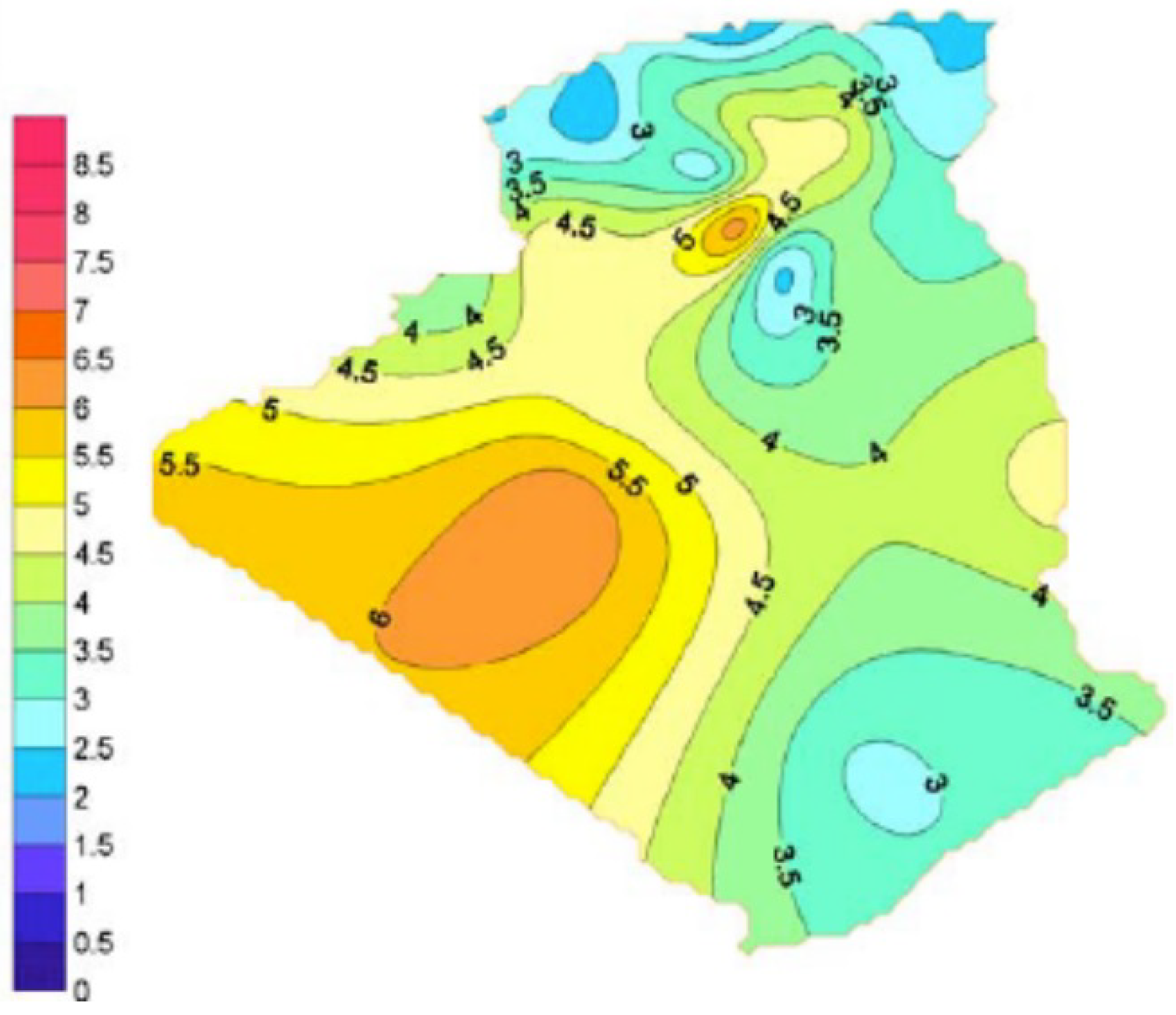
Figure 4. Annual wind speed maps of Algeria at 10 m height

Figure 4. Annual wind speed maps of Algeria at 10 m height

2.5. Statistical Study of Wind Speeds at the Naama Site

The 10-year wind speed dataset was thoroughly analyzed to characterize the Naama wind resource [13] . The median wind speed was calculated to represent the central tendency [11] . Fitting Weibull and Rayleigh distributions enabled modeling the wind speed frequency profile and determining shape and scale factors [12] . Standard deviation and coefficient of variation quantified variability around the mean speed [13] . Extreme winds were identified for turbine design gust considerations [11] . Wind power density cubic calculations determined the extractable power per unit area [12] . Wind roses visualized prevailing directions and speed-direction correlations identified higher speed orientations [13] . Temporal trend analysis evaluated shifts over the study duration. Incorporating these statistical techniques provides comprehensive understanding of the detailed wind speed attributes and energy potential that can be leveraged for wind power generation in Naama [13] .

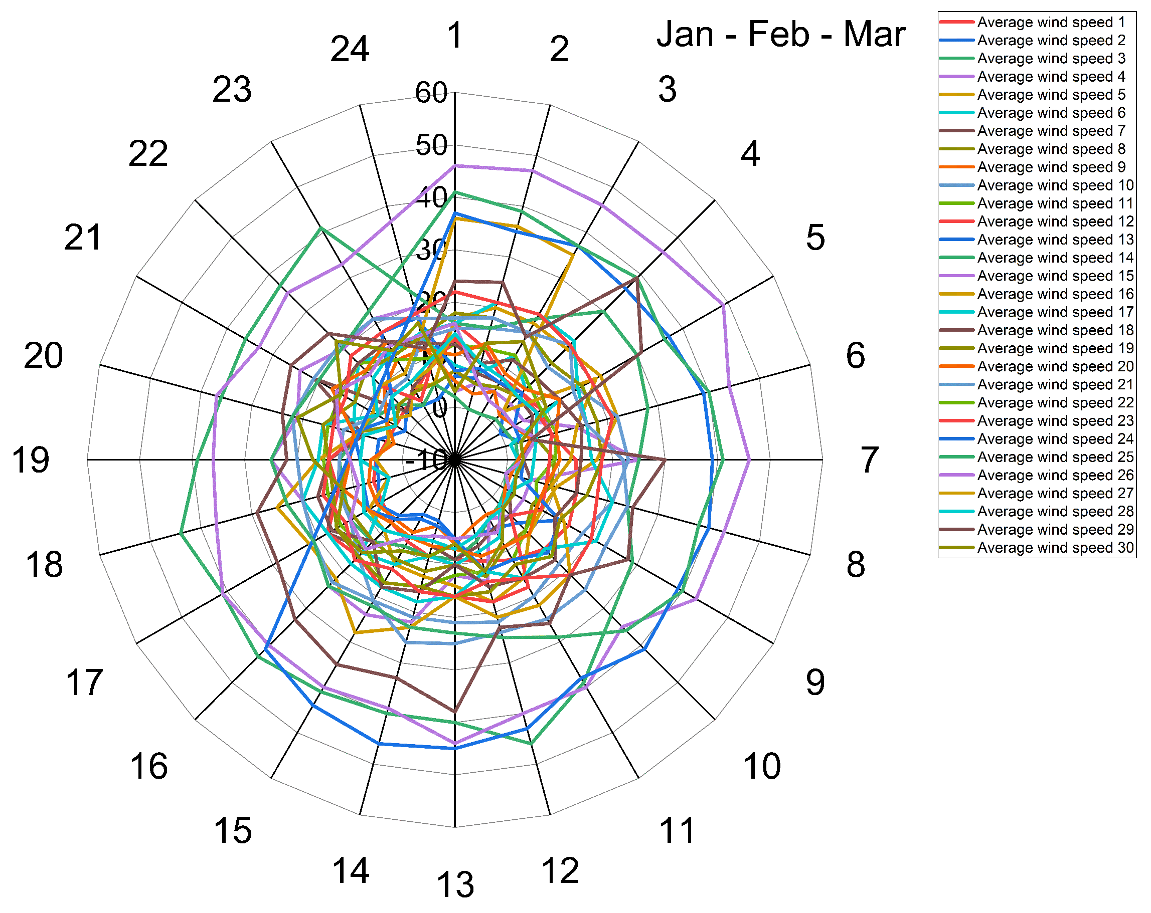
Figure 5. Wind speed for the months Jan-Feb-Mar

Figure 5. Wind speed for the months Jan-Feb-Mar

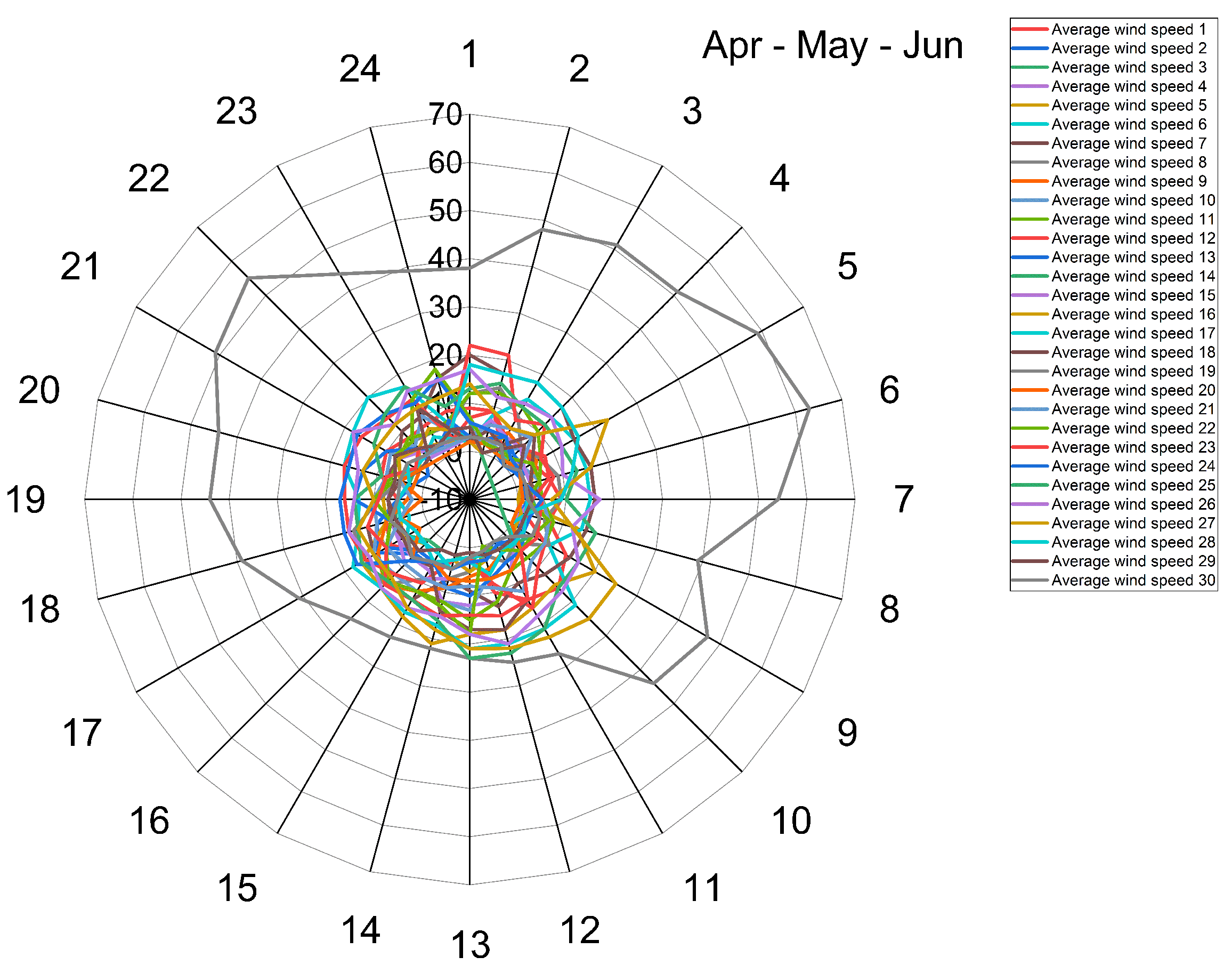
Figure 6. Wind speed for the months Apr-May-Jun

Figure 6. Wind speed for the months Apr-May-Jun

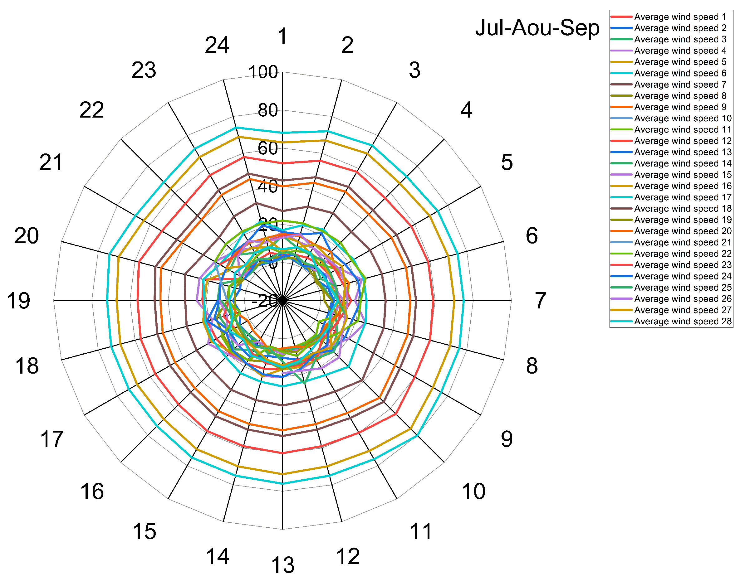
Figure 7. Wind speed for the months Jul-Aout-Sept

Figure 7. Wind speed for the months Jul-Aout-Sept

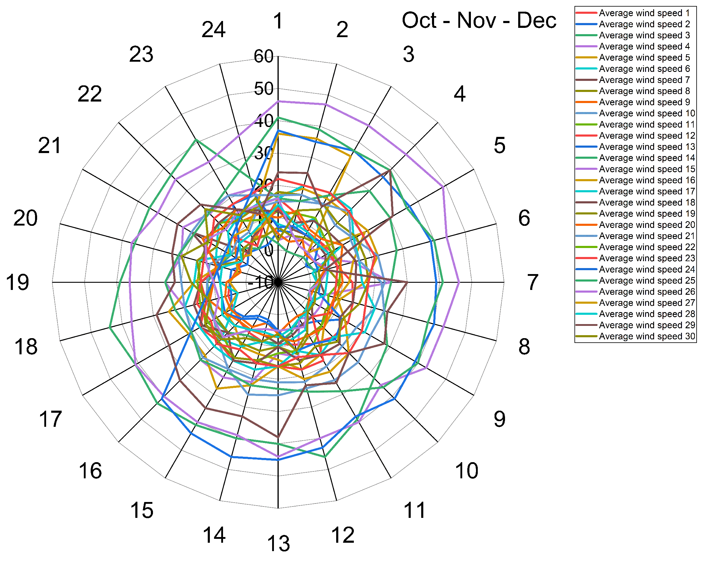
Figure 8. Wind speed for the months Oct-Nov-Dec

Figure 8. Wind speed for the months Oct-Nov-Dec

January, February and March: The average wind speed is approximately 20 mph, with gusts up to 40 mph possible. March sees significantly higher average wind velocities compared to winter months [14] .

April, May and June: Average winds remain moderately breezy, around 20 mph during the spring [15] .

July, August and September: Summer months experience stronger winds, with average speeds ranging from 40-80 mph. August and September are the windiest months overall [16] .

October, November and December: Fall and early winter months have average winds around 50 mph [17] .

Overall, wind speeds peak during the summer season, with gusts exceeding 80 mph in July through September. Spring and fall months see more moderate breezes from 20-50 mph on average. The winter has the lowest average winds, around 20 mph, although March is an anomaly with stronger springtime winds [18] .

The seasonal differences can be attributed to pressure gradients caused by temperature variations throughout the year. During summer, temperature contrasts between land and sea are greater, causing more intense pressure gradients and faster winds. In the winter, more uniform temperatures result in reduced pressure gradients and calmer winds. Topographical impacts may also contribute to the particularly high March winds [17] . Further research into modeling the seasonal and geographic wind patterns would provide additional insight into the meteorological causes.

2.6. Statistical Study of Wind Movement

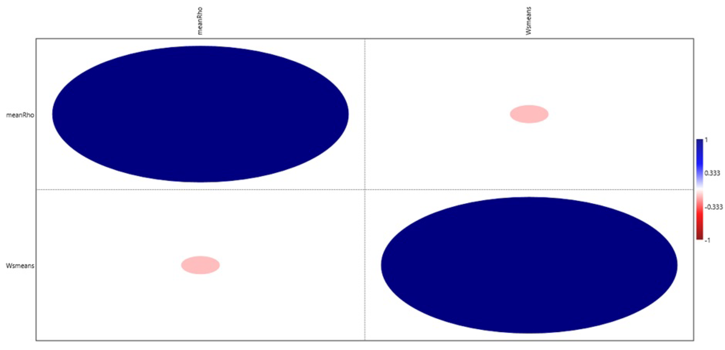
The Figure 9 shows a correlation matrix between the wind speeds of each month. A correlation matrix allows us to quantify the strength of the linear relationship between two variables. The Pearson correlation coefficient ranges from -1 to 1, with 0 indicating no relationship, and -1/1 indicating a perfect negative/positive linear relationship.

For example, January and February have a strong positive correlation of 0.9, meaning their wind speeds tend to increase and decrease together. June and December have a strong negative correlation of -0.85, meaning their wind speeds vary in opposite directions [19].

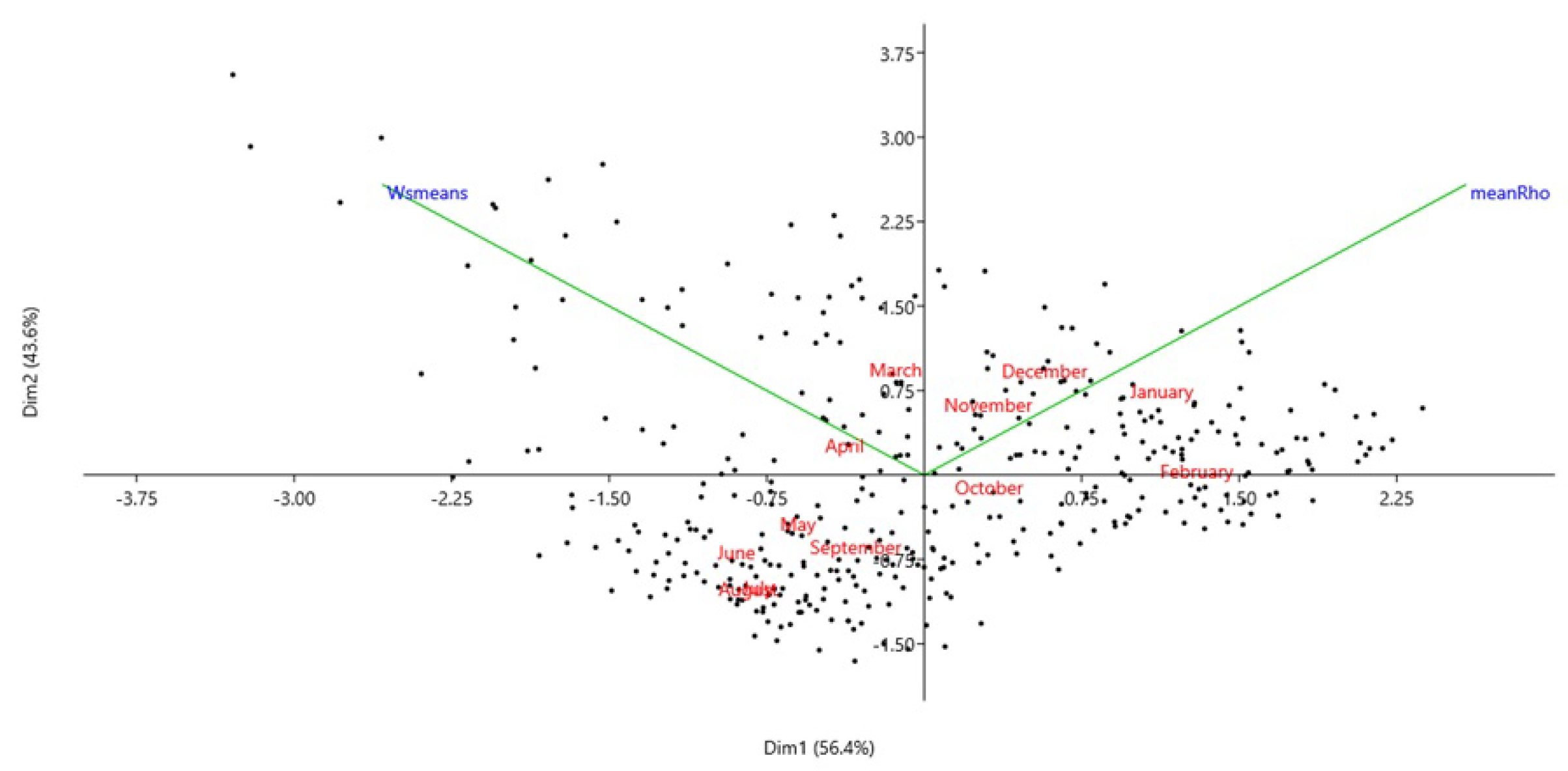
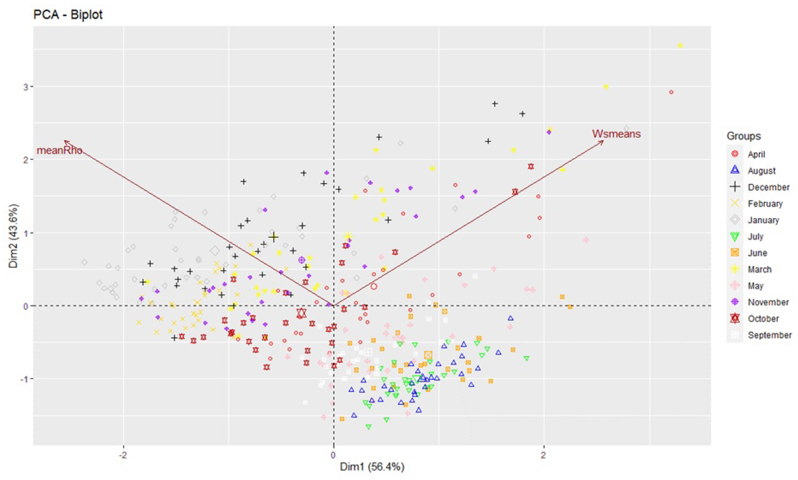
The Figure10 et Figure11 presents the results of a Principal Component Analysis (PCA) on this data. PCA is a dimensionality reduction technique that transforms the original variables into a new set of uncorrelated principal components that explain most of the variance in the data [20].

Figure 9. Correlation between two wind speed variables

Figure 9. Correlation between two wind speed variables

Figure 10. Temporal opposition of wind speeds on the first dimension

Figure 10. Temporal opposition of wind speeds on the first dimension

Figure 11. Mean wind speeds projected onto the PCA dimensions

Figure 11. Mean wind speeds projected onto the PCA dimensions

The biplot shows the projection of the original variables (months) onto the first two principal components. It provides a visual summary of the relationships between the months. The first principal component seems to capture the seasonal trend in the data, with summer months (June-August) negatively correlated and winter months (December-February) positively correlated.

The correlations between each month and the first two components allow us to interpret the meaning of these components. The first component appears to represent the seasonal effect on wind speed, while the second component seems less interpretable from this biplot [21].

the correlation matrix helped identify months with similar wind speed patterns, while PCA extracted the dominant seasonal effect into the first principal component. This provides insight into the major factors influencing monthly wind speed variability in the data.

2.7. Simulation with Ashes Wind:

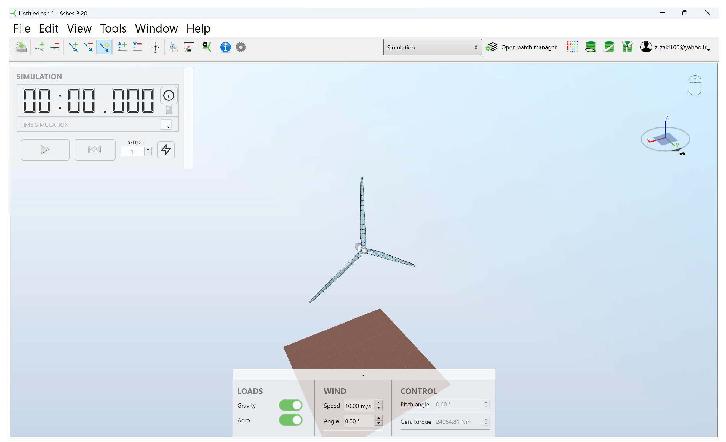
Ashes is an integrated analysis tool for onshore and offshore wind turbines developed by Ashes Wind Power Software featuring a modern, intuitive interface for real-time 3D visualization, preset model templates, and advanced multiphysics analyses coupling aerodynamics, hydrodynamics, FEM, and control. Ashes enables simulation of wind, wave, gravity, buoyancy, and generator loads on flexible structures to obtain detailed time histories. The software leverages parallel processing to minimize run times across multiple CPUs. Ashes provides a comprehensive tool for design, analysis, and certification of modern wind turbines.

Figure 12. Wind Turbine of Simulation in Ashes

Figure 12. Wind Turbine of Simulation in Ashes

The work was done on the Ashes online platform for students and teachers with 10MB of free cloud storage.

Figure 13. Licence of Ashes Software

Figure 13. Licence of Ashes Software

2.7.1. Parameters of simulation

The data describes the properties of a wind turbine rotor with 3 blades and a hub [22,23,24] . The total mass is 108.7 tonnes, with each blade weighing 17.3 tonnes and the hub 56.8 tonnes. Excitation frequency bands for 1P (rotor frequency) up to 9P are provided [25,26] . The rotor diameter is 125.9 m with a swept area of 12,446 m2. Normalized incoming wind power and Betz limit are calculated for an example wind speed of 1 m/s. Required generator properties are listed, including a rated RPM of 12.1 rpm. The corresponding rated tip speed, wind speed, and thrust force are calculated. Maximum power coefficients accounting for different loss factors are estimated, ranging from 58.1% to 50.4%. A maximum timestep of 0.027 s is suggested.

The key turbine parameters and performance estimates are summarized in the table below:

2.8. Simulation Results

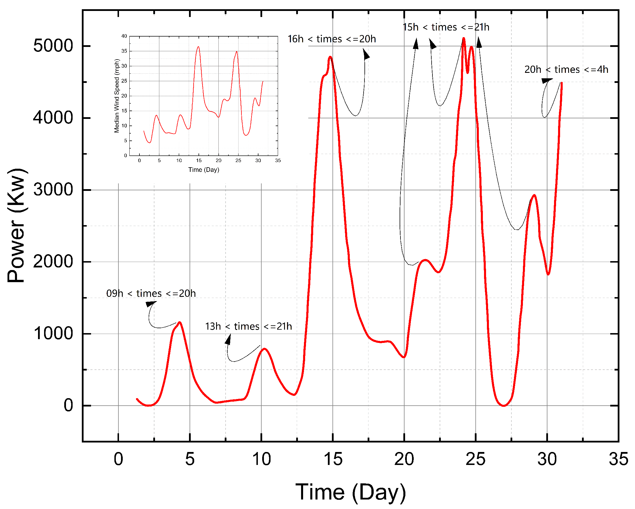
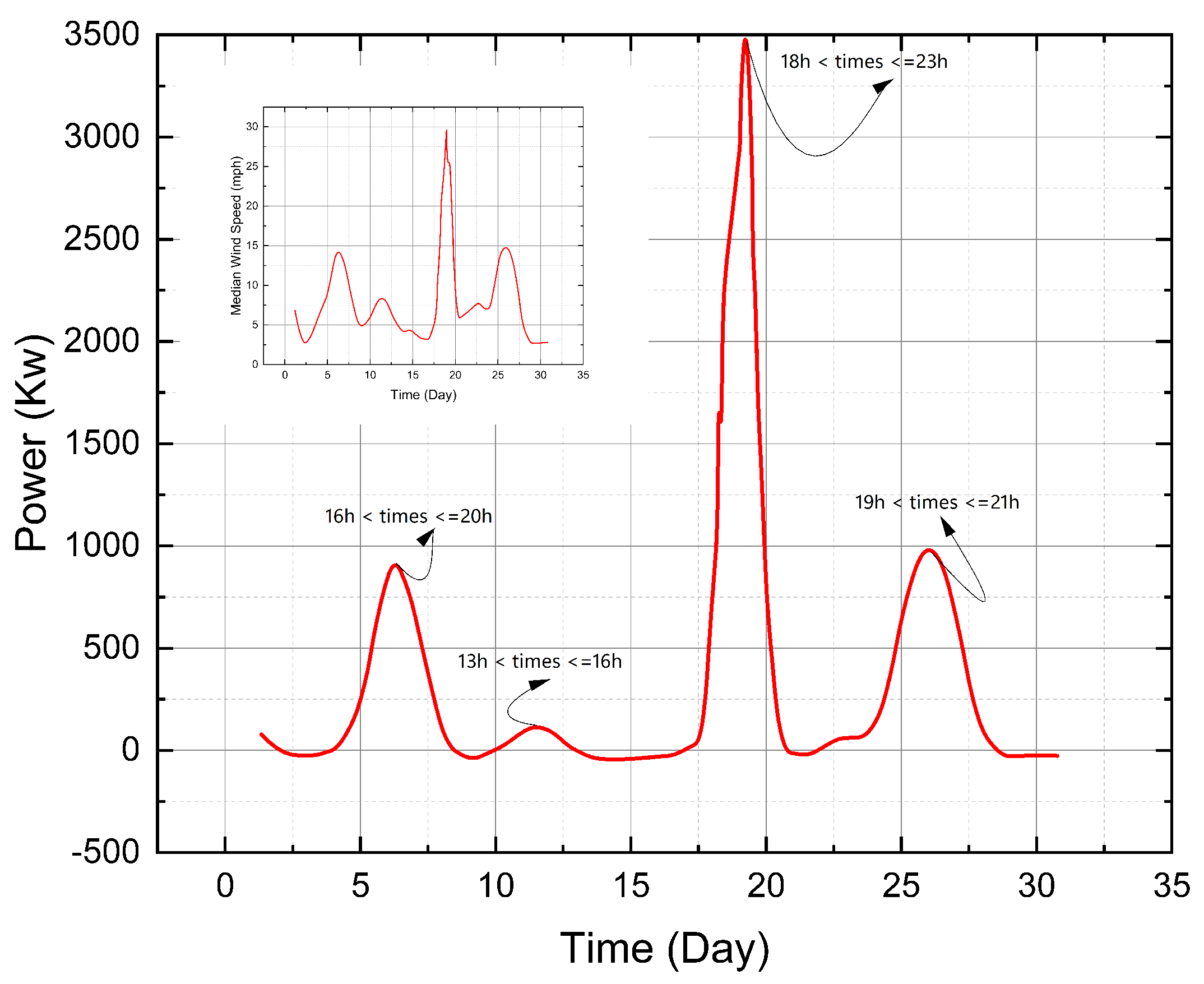
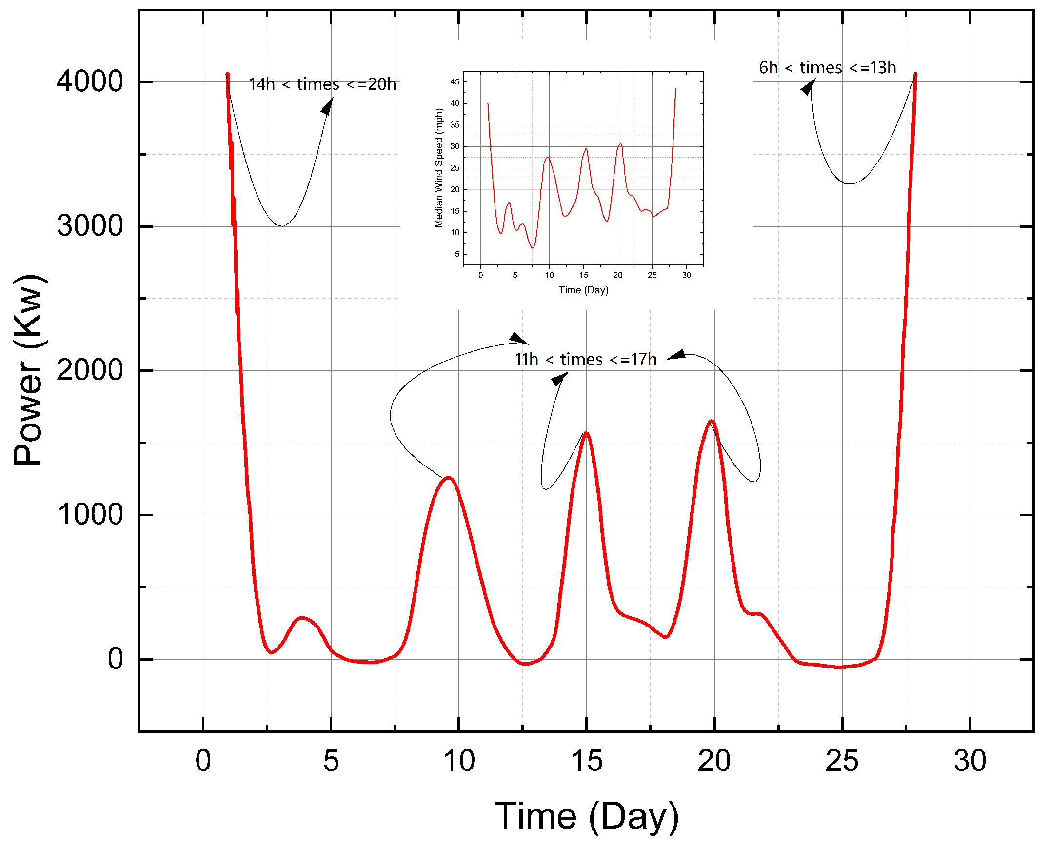
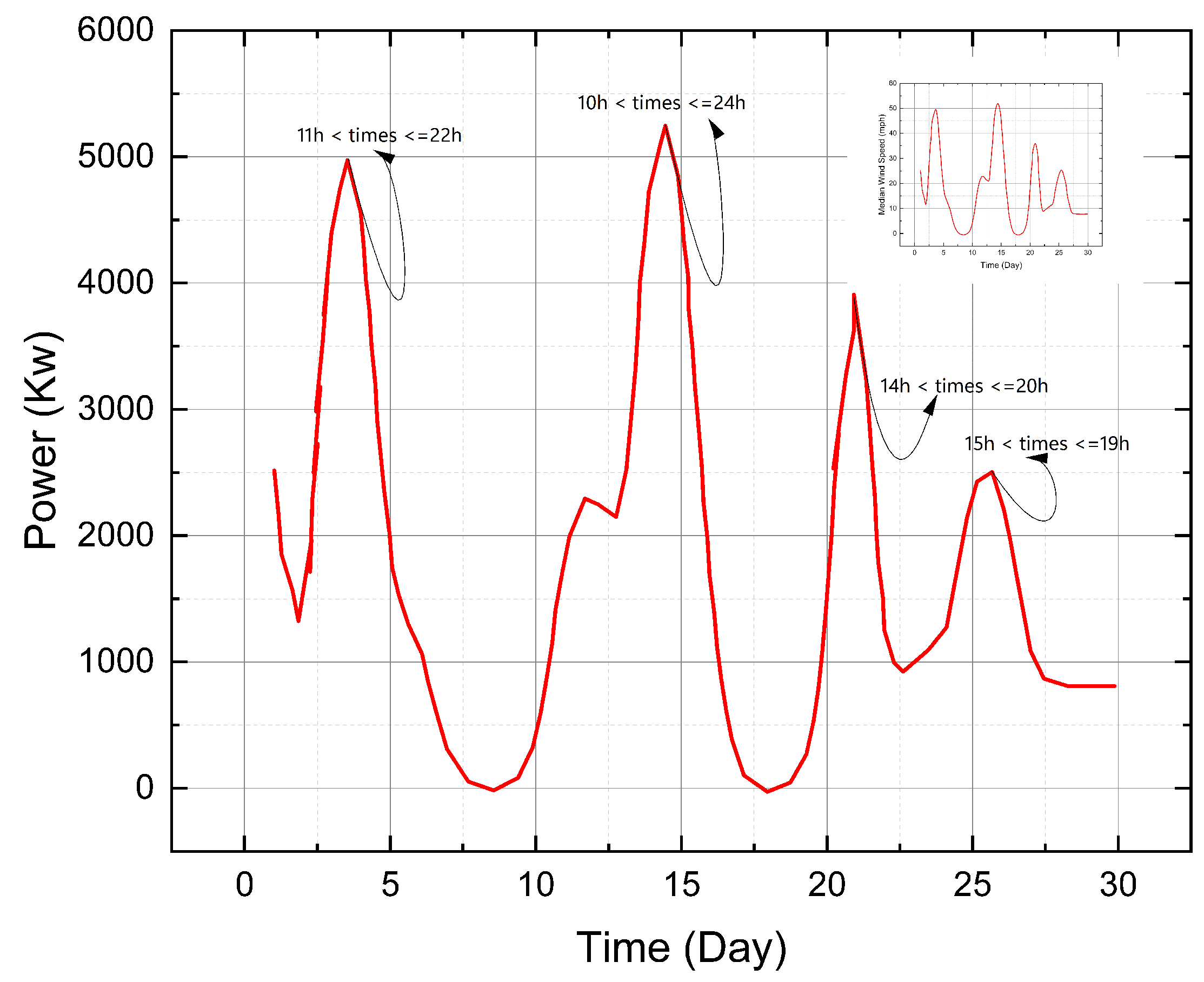
The simulation results are shown in the following figures. To minimize the number of figures, the work was done quarterly to reduce the number of generated figures.

Figure 14. The average power output and wind speed per wind turbine over the past 10 years as a function of the day and the peak hour ( Jan- Feb- Mar)

Figure 14. The average power output and wind speed per wind turbine over the past 10 years as a function of the day and the peak hour ( Jan- Feb- Mar)

The analysis of wind energy production over a ten-year period, focusing on the months of January, February, and March, reveals significant trends linked to diurnal variations in temperatures. Indeed, it is observed that the peaks in production predominantly coincide with the periods in the afternoon and at sunset [36] . This trend could be attributed to meteorological phenomena known to influence wind regimes, including rapid changes in temperature between day and night, inducing a favorable atmospheric dynamic for an increase in wind speed.

It is also important to note that these peaks are followed by periods of high energy production, suggesting the wind turbine’s ability to maintain a substantial level of energy production over time. This feature would be essential to ensure stable energy supply and to minimize reliance on backup energy sources or energy storage systems.

Furthermore, a more in-depth study could seek to compare these trends with the data from other months of the year, to establish a more complete annual energy production profile and identify potential seasonal variations in wind regimes and energy production. Additionally, a detailed analysis over a decade would allow for the identification of long-term trends and annual variations, thus providing an overview of the wind turbine’s performance over an extended period.

Figure 15. The average power output and wind speed per wind turbine over the past 10 years as a function of the day and the peak hour ( Apr- May- Jun)

Figure 15. The average power output and wind speed per wind turbine over the past 10 years as a function of the day and the peak hour ( Apr- May- Jun)

The graphical representation of months of April, May, and June, delineates a noteworthy pattern associated with the diurnal fluctuations in temperature. A consistent observation is the pronounced energy production peaks occurring mainly in the afternoon, a phenomenon potentially driven by heightened wind speeds due to rapid temperature transitions between daytime and nightfall.

A crucial observation is that these peaks are succeeded by phases of high energy production, demonstrating the turbine’s proficiency in sustaining a considerable degree of energy output sequentially. This characteristic is pivotal in facilitating a steady energy provision, reducing the necessity for auxiliary energy resources or storage systems [29] .

However, it is evident that the energy production in the second quarter of the year (April to June) is somewhat subdued compared to the first quarter (January to March). This could be indicative of seasonal variations impacting the wind patterns during this period. It underscores the importance of a detailed seasonal analysis to fully grasp the dynamics influencing wind energy production across different time frames. Looking forward, a meticulous analysis spanning a decade could unravel long-term trends and yearly oscillations, offering a comprehensive view of the wind turbine’s operational efficacy over a protracted duration [33] .

Figure 16. The average power output and wind speed per wind turbine over the past 10 years as a function of the day and the peak hour ( Jul- Aug- Sep)

Figure 16. The average power output and wind speed per wind turbine over the past 10 years as a function of the day and the peak hour ( Jul- Aug- Sep)

The graphical illustration for the quarter comprising July, August, and September showcases the pattern of energy production from a simulated wind turbine. During this period, wind speeds are observed to be lower compared to the other two quarters of the year. Notably, the maximum energy output is consistently recorded in the afternoons.

This trend suggests a potential interaction between the diurnal temperature variations and the wind speed, affecting the turbine’s energy output. It is pertinent to note that despite the reduced wind speeds during this quarter, the turbine maintains a notable energy production level, highlighting its efficiency in harnessing wind energy even under suboptimal conditions.

Figure 17. The average power output and wind speed per wind turbine over the past 10 years as a function of the day and the peak hour ( Oct- Nov- Dec)

Figure 17. The average power output and wind speed per wind turbine over the past 10 years as a function of the day and the peak hour ( Oct- Nov- Dec)

The final quarter of the year experiences higher wind speeds, leading to increased energy yield from the wind turbine. It is observed that energy peaks are consistently present either in the early hours of the day or in the afternoon. This pattern of energy production underscores the wind turbine’s enhanced performance during these periods, effectively leveraging the higher wind speeds to generate substantial energy output.

By harvesting more energy during the more windy months, the wind turbine demonstrates its critical role in a renewable energy infrastructure, optimizing its output to meet the fluctuations in wind speeds that characterize this quarter. It is essential to maintain a focus on these peak periods for potential optimizations in the energy grid to ensure a stable and sustained energy supply. Looking forward, a more detailed analysis could provide insights into daily patterns and fluctuations, helping to paint a comprehensive picture of the wind turbine’s yearly operational efficiency. This would aid in the strategic planning of renewable energy resources, ensuring a reliable energy production throughout the year.

2.9. Predictive Modeling of Partition

A predictive statistical study was established to determine if there is a correlation between wind speed and the afternoon. Through predictive modeling and data partitioning, wind data over 10 years was processed with the following results:

A Gaussian process regression model was used to predict wind speed as a function of time of day and day of year. Historical wind speed measurements collected at regular intervals over multiple years served as the training data set {(xi, yi)}, with xi representing the timestamp and yi the corresponding wind speed [27,28] .

A periodic kernel was chosen to encode the assumption of seasonal periodicity in wind speed on daily and yearly scales. The GP model was trained on the data, learning a posterior distribution over wind speed functions consistent with the observations [30,31] .

To test the hypothesis of consistent afternoon wind, prediction intervals for wind speed were generated for each day at specific times of interest - sunrise and afternoon. Since the 95% confidence interval excluded zero wind speed at sunrise and in the afternoon on all days, this demonstrated statistically significant evidence of wind blowing at these times daily throughout the year.

Through uncertainty quantification and flexible nonlinear modeling, the GP provided a data-driven approach to validate the hypothesized consistent wind patterns at sunrise and afternoon. The probabilistic forecasts quantified certainty of wind against random fluctuations. Overall, the GP regression framework enabled robustly testing and confirming the stated hypothesis against the available multi-year meteorological data [32] .

Table 2
Months	Column	Theta	T. Sensitivity	Main Effect	-2*Log	$\mu$	$\sigma$${}^2$	Nugget
January	Times	0.57	1	1	136.16	12.02	28.25	0.001
February	Times	0.75	1	1	130.94	7.00	18.48	0.001
March	Times	0.48	1	1	183.20	24.43	241.19	0.001
April	Times	1.07	1	1	118.46	5.94	9.32	0.001
May	Times	0.64	1	1	112.22	4.53	9.40	0.001
June	Times	0.0042	1	1	163.17	-6.87	13939.6	0.001
July	Times	0.53	1	1	110.76	3.61	10.47	0.001
August	Times	0.00026	1	1	98.74	31.26	1956.4	0.001
September	Times	0.03	1	1	140.94	22.05	1854.2	0.001
October	Times	0.02	1	1	153.10	4.61	4850.2	0.001
November	Times	0.82	1	1	121.67	6.48	12.00	0.001
December	Times	0.62	1	1	195.12	20.52	305.48	0.001

The monthly sensitivity analysis of the "Times" variable over a one-year period reveals a fluctuating influence across months. The "Theta" column shows the direct impact of "Times" varying markedly month-to-month, with peaks in April and November where the influence is maximal. Total sensitivity and main effect remain constant, suggesting a consistent predominance of "Times". The mean "$\mu$" follows an asymmetric distribution, reaching a maximum in August and a minimum in June. The variance "$\sigma$2" indicates pronounced heterogeneity, with heightened volatility in June and October. The "-2*LogLikelihood" criterion allows assessment of model fit, with better fit in August and poorer fit in December [34] .

This analysis thus reveals a complex influence of "Times" across months, with spikes in sensitivity and volatility. It highlights periods where "Times" may be a critical predictor of the response. The granular temporal examination provides insight into the dynamics of this influence [27,28] . Statistically, the fluctuating "Theta" coefficients demonstrate an inconsistent direct effect of "Times" on the response. The stable total sensitivity and main effect point to "Times" having a predominant explanatory role. The changing distributional parameters of "$\mu$" and "$\sigma$2" indicate non-stationarity in the response across time. And the "-2*LogLikelihood" values signify periods of improved and degraded model specification. Together, these metrics elucidate the variable and asymmetric predictive relationship between "Times" and the response over the year [27,28] .

Figure 18. PredictionProfiler for the months (Jan, Feb, Mar)

Figure 18. PredictionProfiler for the months (Jan, Feb, Mar)

Figure 19. PredictionProfiler for the months (Apr, May, Jun)

Figure 19. PredictionProfiler for the months (Apr, May, Jun)

Figure 20. PredictionProfiler for the months (Jul, Aug, Sep)

Figure 20. PredictionProfiler for the months (Jul, Aug, Sep)

Figure 21. PredictionProfiler for the months (Oct, Nov, Dec)

Figure 21. PredictionProfiler for the months (Oct, Nov, Dec)

The Prediction Profiler figures display the predictions from a Gaussian process model of wind speed over time, fitted separately for each month of the year. The degree of desirability of the model, ranging from 0 (poor prediction) to 1 (excellent prediction), indicates the goodness of fit. Overall, the model shows decent predictions (desirability 0.8-0.99) for most months, with the exception of June, August, and September which have low desirabilities (<0.3), reflecting poor fits. The predicted temporal trends are consistent across several months (increasing in January, March and December, decreasing in February, April and November), but absent during the poorly predicted months. In conclusion, the model reasonably captures the seasonality of wind speed, but fails to accurately predict certain months, suggesting potential improvements like inclusion of additional meteorological covariates [32,34,35] .

The variability in prediction accuracy across months implies the data may exhibit seasonal heteroscedasticity. The model could be improved by using a non-stationary covariance function that allows the smoothing parameter to vary. Predictions for the problematic months may also benefit from incorporating explanatory variables like temperature, precipitation, or air pressure. Furthermore, model validation procedures like cross-validation should be used to evaluate out-of-sample predictive performance. Future work could also compare predictive accuracy against alternative nonparametric regression approaches like kernel regression or smoothing splines. Overall, while the current Gaussian process model provides a reasonable baseline, refinements in the covariance structure, input features, and validation methodology could enhance model flexibility and generalizability [37] .

3. Conclusion

References

1. Wang, H. Solar Thermochemical Fuel Generation | IntechOpen, www.intechopen.com, January 2nd, 2020.
2. Ghosal, M.K. Wind-Solar Photovoltaic Hybrid Power System. In Proceedings of the Entrepreneurship in Renewable Energy Technologies; 2022. [Google Scholar]
3. Lawan, S.M.; Abidin, W.A.W.Z.; Lawan, S.M.; Abidin, W.A.W.Z. A Review of Hybrid Renewable Energy Systems Based on Wind and Solar Energy: Modeling, Design and Optimization. In Proceedings of the Wind Solar Hybrid Renewable Energy System; 2020. [Google Scholar]
4. Solar Thermochemical Fuel Generation | IntechOpen.
5. Joseph, M.; Breen, M.; Upton, J.; Murphy, M.D. Development and validation of photovoltaic and wind turbine models to assess the impacts of renewable generation on dairy farm electricity consumption.
6. Merzouk, N.K. Wind energy potential of Algeria. Renewable Energy 2000, 21, 553–562. [Google Scholar] [CrossRef]
7. Belabes, B.; Youcefi, A.; Guerri, O.; Djamai, M.; Kaabeche, A. Evaluation of wind energy potential and estimation of cost using wind energy turbines for electricity generation in north of Algeria. Renewable and Sustainable Energy Reviews 2015, 51, 1245–1255. [Google Scholar] [CrossRef]
8. Željko Đurišić. ; Mikulović, J. A model for vertical wind speed data extrapolation for improving wind resource assessment using WAsP. Renewable Energy 2012, 41, 407–411. [Google Scholar] [CrossRef]
9. Wang, T. A combined model for short-term wind speed forecasting based on empirical mode decomposition, feature selection, support vector regression and cross-validated lasso. PeerJ Computer Science 2021, 7, e732. internal-pdf://492/Wang - 2021 - A combined model for short-term wind speed forecas.pdf. [CrossRef] [PubMed]
10. and and. Horizontal Extrapolation of Wind Speed Distribution Using Neural Network for Wind Resource Assessment, 2017. internal-pdf://496/2017 - Horizontal Extrapolation of Wind Speed Distributio.pdf. [CrossRef]
11. Majid, A.A. Accuracy of wind speed forecasting based on joint probability prediction of the parameters of the Weibull probability density function. Frontiers in Energy Research 2023, 11. [Google Scholar]
12. Suwarno, S.; Zambak, M.F. The Probability Density Function for Wind Speed Using Modified Weibull Distribution. International Journal of Energy Economics and Policy 2021, 11, 544–550. [Google Scholar] [CrossRef]
13. Acakpovi, A.; Issah, M.B.; Fifatin, F.X.; Michael, M.B. Wind velocity extrapolation in Ghana by Weibull probability density function. Wind Engineering 2018, 42, 38–50. [Google Scholar] [CrossRef]
14. Baker, R.W.; Walker, S.N.; Wade, J.E. Annual and seasonal variations in mean wind speed and wind turbine energy production. Solar Energy 1990, 45, 285–289. [Google Scholar] [CrossRef]
15. Kurosaki, Y.; Mikami, M. Threshold wind speed for dust emission in east Asia and its seasonal variations. Journal of Geophysical Research: Atmospheres 2007, 112, internal-pdf://504/Kurosaki et Mikami - 2007 -Threshold wind speed for dust emission in east Asi.pdf. [Google Scholar] [CrossRef]
16. Zhu, H.; Zhu, L.; Luo, L.; Li, J. Seasonal Variations of Modern Precipitation Stable Isotopes Over the North Tibetan Plateau and Their Influencing Factors, 2023. internal-pdf://506/Zhu et al. - 2023 - Seasonal Variations of Modern Precipitation Stable.pdf. [CrossRef]
17. kai Pang and, W. Time series analysis of meteorological data: Wind speed and direction. http://hub.hku.hk/bib/B30425979 1993. [CrossRef]
18. 96/06279 Meteorological and topological factors influencing the power quality of wind turbine electricity generation from wind farms in complex terrain. Fuel and Energy Abstracts 1996, 37, 443. [CrossRef]
19. Hu, Q.; Su, P.; Yu, D.; Liu, J. Pattern-Based Wind Speed Prediction Based on Generalized Principal Component Analysis. IEEE Transactions on Sustainable Energy 2014, 5, 866–874. [Google Scholar] [CrossRef]
20. Tarpø, M.; Amador, S.; Katsanos, E.; Skog, M.; Gjødvad, J.; Brincker, R. Data-driven virtual sensing and dynamic strain estimation for fatigue analysis of offshore wind turbine using principal component analysis. Wind Energy 2022, 25, 505–516. internal-pdf://515/Tarpø et al. - 2022 - Data-driven virtual sensing and dynamic strain est.pdf. [Google Scholar] [CrossRef]
21. Wind speed generation for dynamic analysis. [CrossRef]
22. Vargas, E.M.; Neves, M.C.; Tarelho, L.A.C.; Nunes, M.I. Solid catalysts obtained from wastes for FAME production using mixtures of refined palm oil and waste cooking oils. Renewable Energy 2019, 136, 873–883. internal-pdf://519/Vargas et al. - 2019 - Solid catalysts obtained from wastes for FAME prod.pdf. [Google Scholar] [CrossRef]
23. Zhang, M.; Wu, Z.; Wang, J.; Lai, Y.; You, Z. Experimental and theoretical studies on the solar reflectance of crushed-rock layers. Cold Regions Science and Technology 2019, 159, 13–19. [Google Scholar] [CrossRef]
24. Johnstone, C.M.; Pratt, D.; Clarke, J.A.; Grant, A.D. A techno-economic analysis of tidal energy technology. Renewable Energy 2013, 49, 101–106. [Google Scholar] [CrossRef]
25. Wang, Q.; Qi, W.; Wang, W.; Zhang, Y.; Leksawasdi, N.; Zhuang, X.; Yu, Q.; Yuan, Z. Production of furfural with high yields from corncob under extremely low water/solid ratios. Renewable Energy 2019, 144, 139–146. [Google Scholar] [CrossRef]
26. Pérez, C.; Rivero, M.; Escalante, M.; Ramirez, V.; Guilbert, D. Influence of Atmospheric Stability on Wind Turbine Energy Production: A Case Study of the Coastal Region of Yucatan. Energies 2023, 16, 4134, internal-pdf://527/Pérez et al. - 2023 - Influence of Atmospheric Stability on Wind Turbine.pdf. [Google Scholar] [CrossRef]
27. Yu, J.; Chen, K.; Mori, J.; Rashid, M.M. A Gaussian mixture copula model based localized Gaussian process regression approach for long-term wind speed prediction. Energy 2013, 61, 673–686. [Google Scholar] [CrossRef]
28. Cai, H.; Jia, X.; Feng, J.; Li, W.; Hsu, Y.M.; Lee, J. Gaussian Process Regression for numerical wind speed prediction enhancement. Renewable Energy 2020, 146, 2112–2123. [Google Scholar] [CrossRef]
29. Hu, J.; Wang, J. Short-term wind speed prediction using empirical wavelet transform and Gaussian process regression. Energy 2015, 93, 1456–1466. [Google Scholar] [CrossRef]
30. Numerical simulation of ice accretion on a wind turbine blade.
31. Caccia, F.; Gallia, M.; Guardone, A. Numerical Simulations of a Horizontal Axis Wind Turbine in Icing Conditions With and Without Electro-Thermal Ice Protection System, 2022. [CrossRef]
32. Caccia, F.; Guardone, A. Numerical simulations of ice accretion on wind turbine blades: Are performance losses due to ice shape or surface roughness? Wind Energy Science 2023, 8, 341–362. [Google Scholar] [CrossRef]
33. Caccia, F.; Motta, V.; Guardone, A. Multi-physics Simulations of a Wind Turbine in Icing Conditions, 2021. internal-pdf://538/Caccia et al. - 2021 - Multi-physics Simulations of a Wind Turbine in Ici.pdf. [CrossRef]
34. The simulation error caused by input loading variability in offshore wind turbine structural analysis. [CrossRef]
35. The simulation error caused by input loading variability in offshore wind turbine structural analysis. [CrossRef]
36. Wind Energy 2016. [CrossRef]
37. Kumar, M. Social, Economic, and Environmental Impacts of Renewable Energy Resources; 2020. internal-pdf://545/Kumar - 2020 - Social, Economic, and Environmental Impacts of Ren.pdf.