ENN: Hierarchical Image Classification Ensemble Neural Network for Large-Scale Automated Detection of Potential Design Infringement

Preprint

Article

ENN: Hierarchical Image Classification Ensemble Neural Network for Large-Scale Automated Detection of Potential Design Infringement

Altmetrics

Downloads

Views

Comments

A peer-reviewed article of this preprint also exists.

Chan Jae Lee^†,Seong Ho Jeong^†,

Young Yoon^*

Chan Jae Lee^†,Seong Ho Jeong^†,

Young Yoon^*

^† These authors have contributed equally to this work.

This version is not peer-reviewed

Submitted:

16 September 2023

Posted:

19 September 2023

You are already at the latest version

Alerts

Abstract

This paper presents a two-stage hierarchical neural network using image classification and object detection algorithms as key building blocks for a system that automatically detects a potential design right infringement. This neural network is trained to return the Top-N original design right records that highly resemble the input image of a counterfeit. Design rights specify the unique aesthetic characteristics of a product. Due to the rapid change of trends, new design rights are continuously generated. This work proposes an Ensemble Neural Network (ENN), an artificial neural network model that aims to deal with a large amount of counterfeit data and design right records that are frequently added and deleted. At first, we performed image classification and objection detection learning per design right using the existing models with a proven track record of high accuracy. The distributed models form the backbone of the ENN and yield intermediate results aggregated at a master neural network. This master neural network is a deep residual network paired with a fully connected network. This ensemble layer is trained to determine the sub-models that return the best result for a given input image of a product. In the final stage, the ENN model multiples the inferred similarity coefficients to the weighted input vectors produced by the individual sub-models to assess the similarity between the test input image and the existing product design rights to see any sign of violation. Given 84 design rights and the sample product images taken meticulously under various conditions, our ENN model achieved average Top-1 and Top-3 accuracies of 98.409% and 99.460%, respectively. Upon introducing new design rights data, a partial update of the inference model was done an order of magnitude faster than the single model. ENN maintained a high level of accuracy as it scaled out to handle more design rights. Therefore, the ENN model is expected to offer practical help to the inspectors in the field, such as the customs at the border that deal with a swarm of products.

Keywords:

Subject: Computer Science and Mathematics - Artificial Intelligence and Machine Learning

1. Introduction

Industrial design involves creative activities to reasonably and organically construct various product elements. Such designs can be protected by law by applying design right registration. This paper is keen on the problem of the registered design rights being violated by delicately imitated products. Non-experts may not easily distinguish between the original design of a genuine product and a fake one. The illegal counterfeit products continue to increase, causing unfair damage to the product design rights owners. According to an OECD report [1], the annual damages due to piracy amounted to 500 billion US dollars. To prevent such damage, professionally trained human inspectors at customs manually inspect for illegal forgery of goods coming from overseas. If a product is suspected to be an unlawful copy during the screening process, it is seized for further investigation of its authenticity. However, even for inspectors with years of experience, it is overwhelming to compare the large volume of incoming products against the list of thousands of design rights. Therefore, an automated illegal counterfeit probe system is in great need.

Artificial intelligence (AI) recently has advanced unprecedentedly with the introduction of some foundation models that were proven to be effective in various problem domains [2,3,4,5]. Some AI technologies have been employed for small-scale counterfeit examining systems [6,7,8]. However, the proposed neural networks still have several limitations in building an automated system for examining counterfeit copies at a large scale. The design rights are an aesthetic element that constantly and rapidly change to stay current with the trend. Therefore, new design rights are frequently registered. Enabling a more prompt machine learning system is imperative to cope with outpouring products against thousands of continually changing product design rights.

Upon introducing new design rights and the associated training image data, most methodologies perform transfer learning of the existing model. The re-learning cost increases proportionally to the number of design rights, thus hampers realizing a scalable counterfeit examining system.

This paper is intrigued by the mechanism of the neocortex in human brains as explained in [9,10]. In [10], it was confirmed that the brain’s neocortex operating as a single mechanism comprises six layers and a column of neurons with a vertical structure penetrating the layers. Also, in [9], it was revealed that neuron columns collectively solve the problem through a consensus process to learn the world model holistically. Based on the mechanism of the actual brain operation, we devised a distributed sub-neural network model analogous to the vertically configured neuron column. Then, we created a master neural network that aggregates the intermediate results produced by the distributed sub-models and selects one that returned the best classification result for a given test image. This ensemble layer’s work is analogous to the voting mechanism in the neocortex. We refer to such stepwise hierarchical neural network structure as ENN (Ensemble Neural Network).

At first, the product images of design rights were segmented into non-intersecting groups. For each group, we employed a sub-neural network model proven effective for image classification and object detection. The master model at the succeeding stage collects the individually trained sub-models’ output and takes them as input to learn their weights. After completing the stepwise learning process, the ENN model multiples the inferred weight values to the weighted input vectors produced by the individual sub-models to assess the similarity between the test input image and the existing product design rights to find any sign of violation.

Figure 1 illustrates the overall structure of an automated system for examining counterfeit products based on image-examining technology using AI. This system transmits the input image taken via client API to the ENN model. The ENN model returns the Top-N similar product design rights. This system also yields a unique article number of similar design rights. A given product that exceeds the similarity threshold is suspected of violating an existing design right, and the image capture of the alleged product is sent to the design right holder via email. This paper discusses the ENN model, which sits at the core of the counterfeit screening system.

The critical characteristic of ENN is the hierarchical neural network structure that combines the results of segmented learning by the sub-models. When a sub-model for the newly introduced design rights is added to ENN, there is no need to pull up the training data of other design rights all over again to complete the classification learning procedure. Therefore, the learning cost of ENN is significantly lower than that of a single model. The master model still conducts the transfer learning upon completing the newly introduced sub-model. However, the master model does not directly output similarities for the entire classes. Instead, the master model learns to output the relevancy of the sub-models for a given sample product image.

Given 84 design rights and the sample product images taken meticulously under various conditions, our ENN model achieved average Top-1 and Top-3 accuracies of 98.409%

This paper is structured as follows. Section 2 first reviews the related research works. Section 3 introduces ENN, the core hierarchical neural network model for the automated design right violation detection system. Section 4 discusses the experimental results. Finally, we reach conclusions in Section 5.

2. Related Works

Illegal replicas are spreading rapidly due to technological advances in logistics. Accordingly, various methods have been proposed for detecting such counterfeiting through various methods [6,7,8,11]. Among them, a way to automatically calculate the probability that a product is a counterfeit based on online customer reviews in the market has been proposed [11]. This study used natural language processing (NLP) and subject analysis methods to process customer reviews. This work also defined counterfeit scores. However, these approaches depend on the NLP analysis of buyers’ reviews that become available only after a specific purchase. Therefore, such a method cannot be exercised at the forefront of product screening before distribution. Diversified sales routes evading customer reviews can result in more victims. Thus, a preventive measure should be applied well before the counterfeits enter the market.

There is a limit to the supply of professional human resources to respond to the increasing number of counterfeits. Moreover, it is difficult for customs to unpack and dissemble items arbitrarily for further inspections. This issue calls for a non-destructive inspection method. The most basic non-destructive testing method is to analyze the visible characteristics. It is possible to analyze specific patterns through an AI-based computer vision algorithm. In particular, impressive performance is shown by image classification and object detection algorithms as presented in [12,13,14,15].

AI-based computer vision technologies have emerged in the studies of the detection of counterfeit bills [6,7] and logos [8]. These studies are limited to recognizing the similarity with a single genuine item. Such special-purpose inspection methods are inappropriate for our case, where a given object has to be compared against multiple categories, i.e., design rights. Counterfeit screening becomes more challenging as new product design rights are constantly added and updated. Despite transfer learning [16], the learning cost increases exponentially with the number of classes if a single model is used for classification.

We devised distributed backbone neural network models ensembled to form a master model and efficiently deal with frequently updated design rights at a large scale. The ensemble model has been studied to improve the accuracy of a single model [17,18,19] in the image classification domain. Besides more classical approaches such as voting [20], bagging [21] and boosting [22], stacking has recently shown some effectiveness for image classification [23]. Some stacking methods used a sequence of different models [22,24]. Another stacking method applied the same data to different models at once and aggregated the results [25]. More recently, the backbone structure has emerged [14,15]. However, these ensemble approaches incur a cost that increases exponentially with the number of classes. All backbone models have to be re-trained even to reflect incremental training data updates. Contrary to these previous approaches, we aim to support incremental updates to achieve high scalability while maintaining high classification accuracy.

3. Methodology

Previous studies had limitations on responding to the continuous addition of design rights. We employed the core idea for addressing such limitation by designing a neural network similar to the human brain structure studied by Jeff Hawkins and Mountcastle [9,10]. In particular, as mentioned in [10], we tried to construct a sub-neural network that acts similarly to a cortical column of a vertical structure following a common mechanism. We propose a distributed backbone neural network structure functioning as a neural pillar and learns independently per design rights partition. Such an approach differs from the existing learning methodology that applies a single neural network to the entire dataset.

Given the inference result by vertical neuron pillars, we propose a two-level structure of ENN in which the parent or master neural network derives the final consensus for learning the world model. Such partitioned learning and stepwise conclusion at the master layer mimics the human neocortex neuronal columns that vote to retain the world model as mentioned in [9]. Learning sub-networks upon introducing new data classes is much faster than re-training the entire network. With our ENN, re-learning is done only at the master layer that only takes the input from the newly trained sub-networks. Therefore, ENN can scale to many output classes. In the following, we look more deeply into the architecture of the ENN model.

3.1. Model architecture

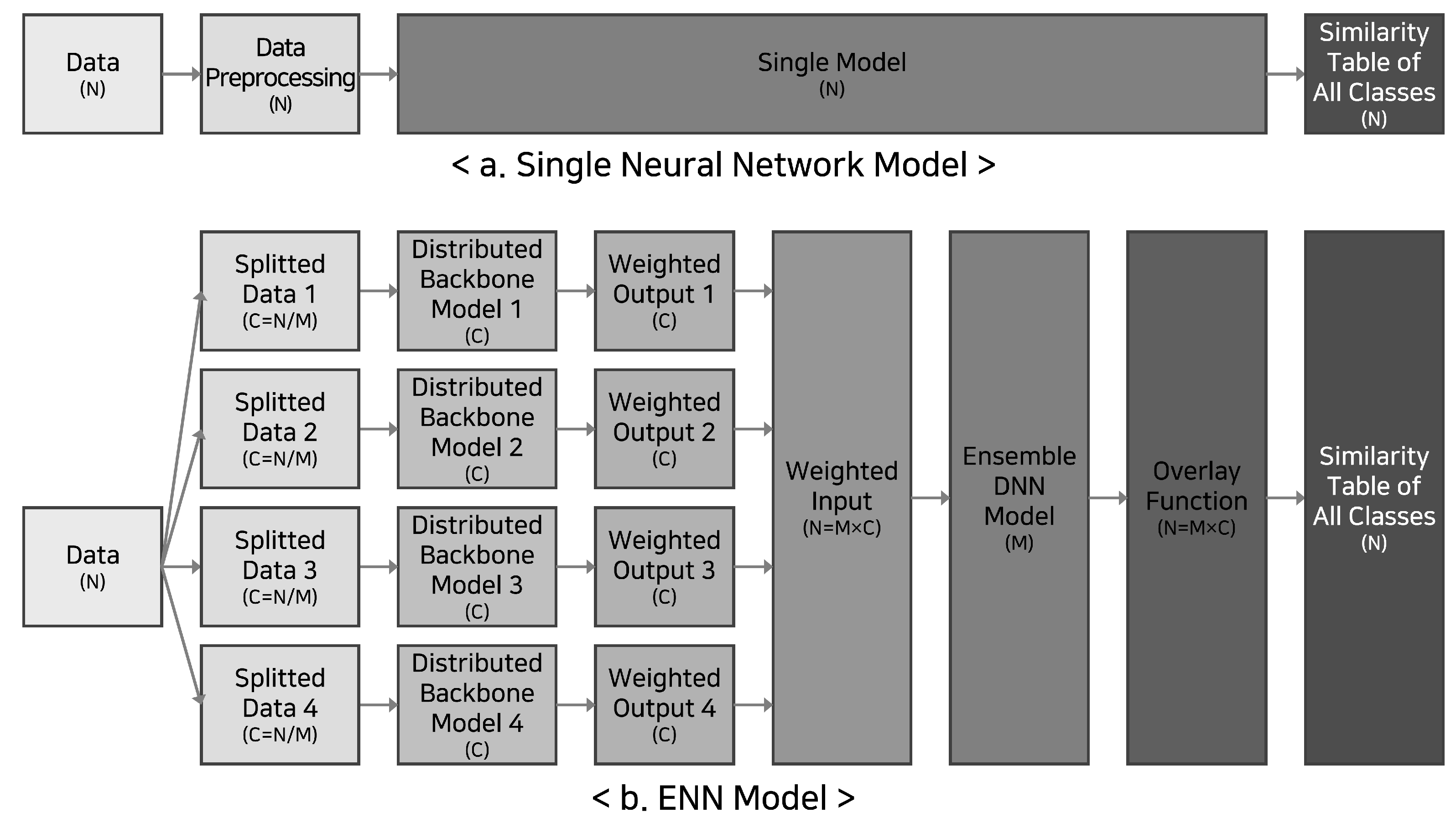
Figure 2 compares our ENN model against the conventional single models. First, Figure 2.a describes the existing approach method of injecting preprocessed input data through a network of a single structure. The neural network performs an examination operation for a given product image through a sufficiently learned single network and finally outputs the similarity for all classes. Figure 2.b has a similar structure to Figure 2.a, except that it uses distributed backbone models and an ensemble layer that makes a final selection by combining the intermediate results from the backbone models. Looking closer, the input data are partitioned into N groups. Each group passes through M sub backbone neural network models. Subsequently, the output of the sub-models is concatenated and passed through the ensemble layer following a Deep Neural Network (DNN) structure. We refer to this ensemble layer as a master or a parent layer. In the last step, the similarity for all final design rights is returned by an overlay function that takes the product of the ensemble model result and the weighted tensor. The ENN model proceeds through the following five steps to learn the design rights of a given product image.

First, the ENN receives an image and performs augmentation, including input size adjustment and normalization.
The ENN outputs a distributed weighted output through a distributed backbone neural network.
The ENN concatenates the distributed weighted outputs of the individual sub-neural networks and converts them into weighted inputs tensor to be passed to the master layer.
With weighted input tensor as input, the ENN computes the order similarity coefficient for each backbone model
The ENN multiplies the weighted input tensor and the similarity coefficient tensor to output the final closeness of an input image to every design right.

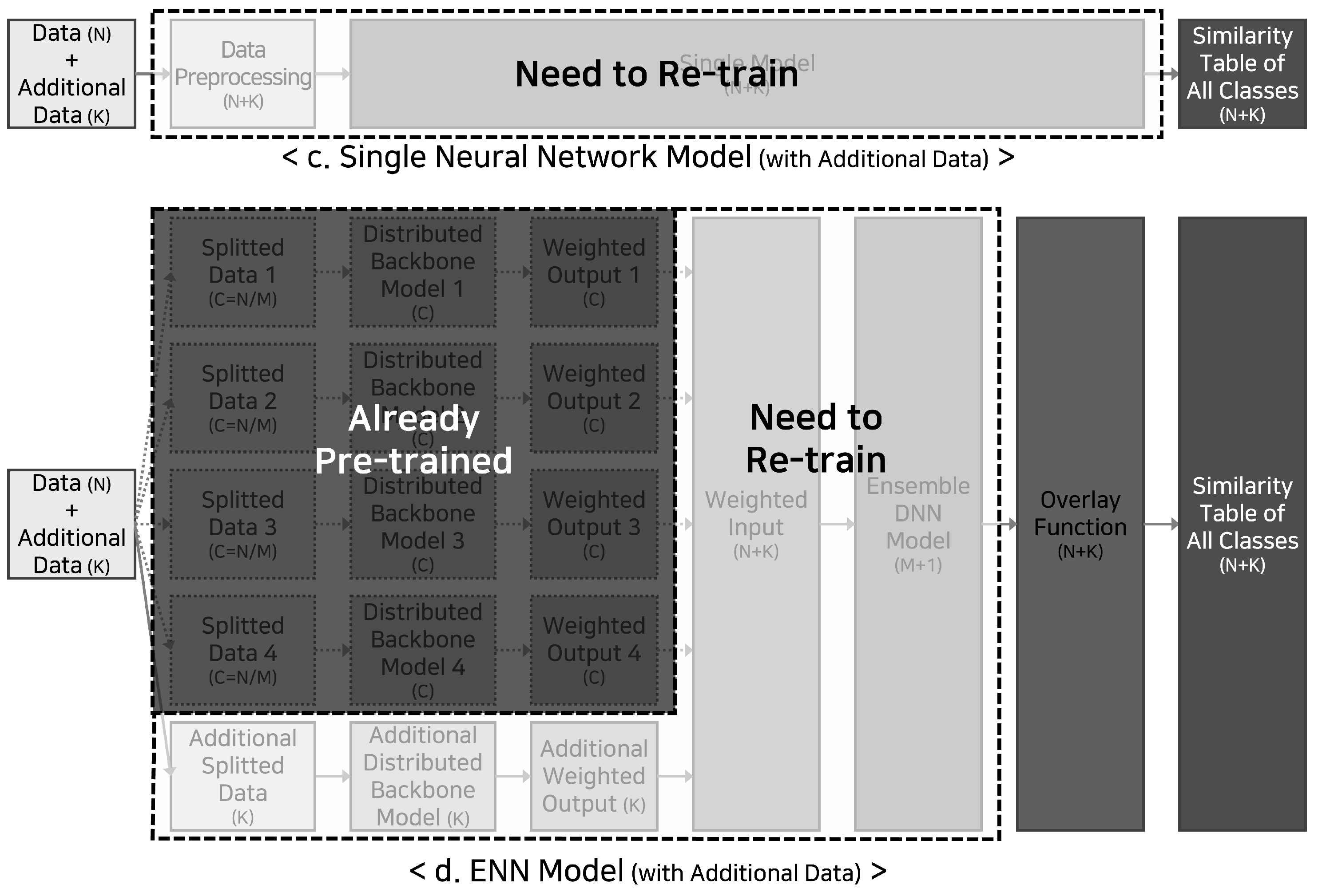
Figure 3 represents the re-learning operation that should run due to introducing new data. Previous studies, such as the one shown in Figure 3.c require transfer learning of the entire model when a set of design rights is added. For the ENN model we proposed, as shown in Figure 3.d, only the backbone model designated for the new data set goes through the training phase. The DNN model at the master layer picks up the result from the new backbone model and goes through the partial transfer learning. Training time can be significantly reduced since the previous backbone models remain unchanged.

3.1.1. The distributed backbone model

As mentioned in [10], the core of the ENN model is a distributed backbone model that acts similarly to a cortical column of neurons that follow a near-identical structure. The main idea of a distributed backbone model is to learn per partitioned data set. In this study, the initial dataset was divided to have the same number of classes (design rights) as much as possible. There is no overlap in design rights between different distributed backbone models. Distributed neural networks can be trained independently and quickly in parallel.

Suppose there is a set of 50,000 image data and 100 design rights. Each design right is associated with 500 image data. Suppose we segment the 100 design rights into five superclasses, each class having 20 design rights. Then, the first model can learn with 10,000 images corresponding to 1st–20th class, and the second model can learn with 10,000 images corresponding to 21st–40th class. Likewise, the rest of the models perform the distributed training individually by dividing the data by 10,000 images each.

The main reason for learning per divided dataset is to overcome the inefficiency of the existing methodologies that typically train on one huge neural network. The single network model incurs a significant cost of transfer learning on the entire data. Existing methods train one huge neural network to learn all classes, and additional training requires transfer learning over the whole data even when new data are incrementally added. However, our ENN model can be trained on the entire class much quicker by training only the distributed backbone model affected by the change to the dataset. We can even benefit from parallelism by simultaneously training the required distributed backbone models on separate devices.

Assume a hyper-scale neural network that needs to be trained to classify an input into more than 500,000 design rights. If there are 500 images per design right, then the single neural network model is trained with about 25 million images per epoch, even when only one class was newly added, and the rest of the data were trained in advance. Moreover, the depth of the neural network may also have to be significantly re-scaled and re-calibrated to avoid any possible underfitting problem when the number of classes becomes very high. Therefore, learning with a single neural network is inappropriate for our problem of dealing with many product types.

In the case of ENN, each distributed backbone model receives a learnable workload for a more feasible model fitting. Suppose one backbone model can comfortably learn up to 1,000 classes of data. For 50,000 classes, we can have 500 backbone models trained independently on different devices. If 100 extra classes are introduced, we can designate one backbone model to learn from the new train data and let it pass the weighted input to the ensemble DNN model. The other backbone models pre-trained on the previous 50,000 classes do not have to be re-trained. The re-training at the ensemble DNN layer (the master layer) is done quicker than the single neural network model as it only needs to account for the weighted input of the newly trained distributed backbone models. Therefore, the ENN model only incurs learning costs proportionally to the amount of the new data.

3.1.2. The Ensemble DNN model

We provide the microscopic view of the ensemble DNN model in Figure 4. The ensemble neural network model derives a final consensus on the results of the distributed backbone model, just as neurons reach agreement through voting to learn the world model in the neocortex composed of neuron columns, as explained in [9]. The ensemble DNN model takes the initial input with the size of N and returns an output with a size equal to the number of distributed models (M). M is smaller than N as the distributed models are learned on partitioned datasets.

This model first takes a weighted input tensor and injects it into an FC (Fully Connected) Layer. Then, the data is fed forward through a sequence of six FC Residual Blocks that follow the ResNet architecture [12]. Each Residual Block comprises a Batch Normalization Layer, an FC Layer, a Dropout Layer, and an Activation (ReLU) Layer. The output of the preceding block is added to the activation layer of the next block. After the last Residual Block, the Sigmoid function, as defined in Equation (1), is applied. The dimension of the Sigmoid function output is identical to that of the weighted input tensor. The result of the Sigmoid function is multiplied by the weighted input tensor through the overlay function. At this time, the shape of the output is the same as the number of distributed models (N) so that the final similarities of all design rights are obtained.

S i g m o i d (x_{i}) = \frac{1}{1 + e^{- x_{i}}}, i \in 1, 2, 3, . . ., k

(1)

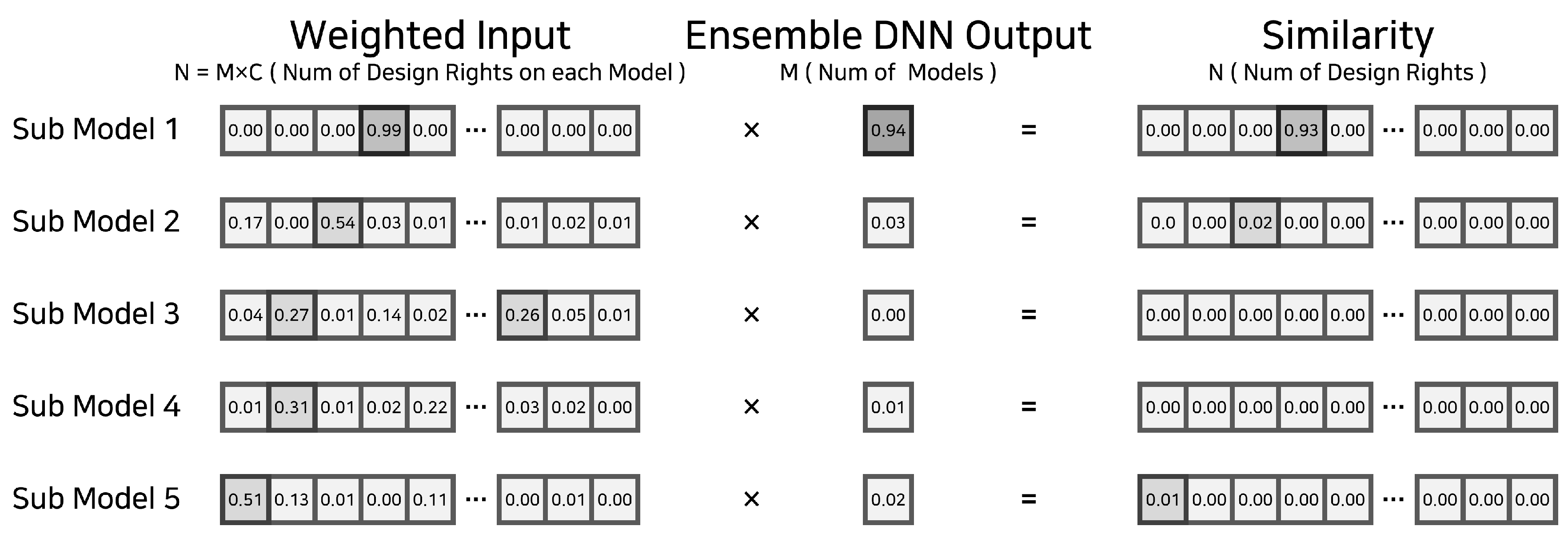
Figure 5 shows that the overlay function is given p weighted input tensors. The overlay function multiplies the similarity coefficient learned by the ensemble DNN model for each input tensor. The similarity coefficient is computed using the Sigmoid or the Softmax function (Equation (2), depending on the model we use for the backbone layer. The design right similarities are in descending order in a P x M matrix. Given the similarity table, we can instantly identify the Top-N design rights the input image is suspected to be related to.

S o f t m a x (x_{i}) = \frac{x_{i}}{\sum_{j = 1}^{k} e^{x_{j}}}, i \in 1, 2, 3, . . ., k

(2)

The ensemble DNN model takes the input as a weighted input tensor containing the results of the preceding variance model and infers which model is the most relevant to the input image according to the similarity coefficient. The order of the preceding distributed models must remain unchanged during training and inference to determine the most pertinent variance model. Since the size of the output is very small compared to the size of the input, the ensemble model is designed to follow a fairly simple structure. When a class is added or changed, the output layer of the ensemble DNN model must be adjusted accordingly, and the re-training process has to be carried out.

Illegal counterfeits can violate multiple design rights. Thus, we should be able to detect various relevant design rights at the same time. How such a requirement is met depends on whether we use the image classification or the objection detection model as the backbone model.

If the backbone model implements image classification, the similarity of each image classification backbone model is returned for every design right. For example, the model learned from one of the five supersets diving 100 design rights yields the similarity of 20 classes. We chose the Sigmoid function over the Softmax function shown in Equation (2) to enable k multiple class detection from a single input image.

On the other hand, the object detection model already identifies multiple class objects in bounding boxes simultaneously within one image. The object detection model uses the Softmax function to predict individual objects’ class (design right) in bounding boxes. In addition, the max value of each class is added to the calculation process as shown in Equation (3) with k as the number of design rights. This process picks a design right with the highest similarity value for the detected object captured in a bounding box.

Backbone models can be substituted flexibly to seek performance gain.

X_{i} = m a x (x_{(i, \forall_{b b o x})}), i \in 1, 2, 3, . . ., k

(3)

Note that the individual distributed backbone models use a deeper architecture than the ensemble DNN model. We could make the ensemble DNN model lighter as it only needs to learn to output the similarity coefficients of the backbone models instead of learning to return the similarity of every design right. With the output of the ensemble DNN model, we can identify a sub-model that is relatively more likely to return the relevant class for a given input image. Most similar design rights can be computed instantly by running the overlay function. We maintain the efficient training and inference process by keeping the ensemble layer simple while minimizing the accuracy compromise.

4. Experiments

This section assesses the performance of the ENN model.

4.1. Experiment setup and implementation

We trained and tested our models on the Dell EMC DSS 8440 server with a 40-core CPU with 80 threads and six Tesla V100 GPUs, each with 32 GB of exclusive memory and 256 GB of RAM. DSS 8440 is operated with Ubuntu 18.04.6 LTS, and the machine learning jobs were executed on Docker containers. We implemented the following machine learning algorithms as the distributed backbone models.

UP-DETR [15] with CUDA (v10.2) Python (v3.7.7), PyTorch (v1.6.0), and Torchvision (v0.7.0)
ResNet [12] with CUDA (v10.2) Python (v3.7.7), PyTorch (v1.6.0), and Torchvision (v0.7.0)
WideResNet [26] with CUDA (v10.2) Python (v3.7.7), PyTorch (v1.6.0), and Torchvision (v0.7.0)
Yolo [13] with CUDA (v10.2) Python (v3.7.7), PyTorch (v1.6.0), and Torchvision (v0.7.0)
EfficientNet [27] with CUDA (v10.2) Python (v3.7.7), PyTorch (v1.10.0), and Torchvision (v0.11.0)

4.2. Data collection and augmentation

We collected 115,916 images for 84 design rights listed in Table 1 and Table 2. More detailed information on the design rights is available on KIPRIS (Korea Intellectual Property Information Search) http://www.kipris.or.kr/khome/main.jsp. Approximately 1,380 images were evenly collected for each of the 84 design rights. For each design right, the models used are also listed. The notation of the model is a tuple followed by an ID indicating a group of design rights. The first and the second elements of the tuple of a model indicate the number of backbone models used and the number of design rights each backbone model learns. For instance, the first design right on Table 1 is a wireless earphone with a unique registration number of 3008346600000. One of the models applied to the train images of this design right was (1,11)A, meaning that one backbone model was used for learning the images of 11 design rights. The letter ’A’ indicates the ID of the group to which this design right belongs. We split the image dataset into train, validation, and test sets in an 8:1:1 ratio.

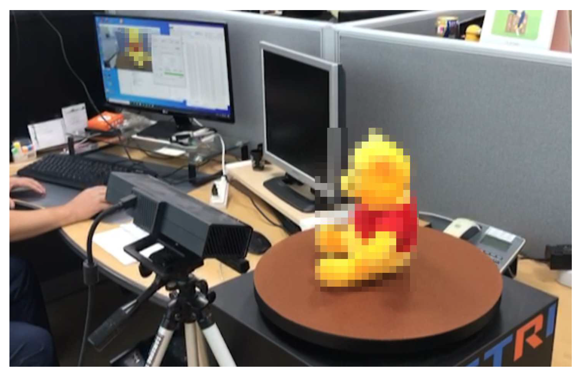
National IT Industry Promotion Agency of Korea acquired the sample products of these design rights. As shown in Figure 6, we used a machine that turns the table to photograph a sample product every three degrees. Camera height was set to high, medium, and low. We set the lighting to bright, standard, and dim. Through this photograph process, we collected 1,080 images per sample product. Additionally, we took 300 pictures of each product under realistic conditions, such as showing the wrapping with label attachments. The human experts in design right examiners annotated ground truth images within bounding boxes.

To obtain more real-world cases, we applied various data augmentation techniques [28,29] such as horizontal reversal, vertical reversal, brightness adjustment, contrast adjustment, saturation adjustment, image size adjustment, normalization, and partial image hiding [30].

Horizontal and vertical inversion were applied with a 50% probability. The brightness, the contrast, and the saturation were randomly selected from the ranges of 0.2–2.0, 0.8–1.2, and 0.5–1.5, respectively. The image length was chosen from 480 pixels to 800 pixels with a unit length of 32 pixels when UP-DETR was used as a distributed neural network. We stroked the best balance between accuracy, training, and test speed when the image length was set to 512 pixels. After applying the commonly used image normalization, a part of the image was covered with a 30%

Through these various image augmentations, we increased the model’s accuracy even with the initial small set of images.

4.3. Comparison of training speed

Table 3 shows the average training time per one epoch using the UP-DETR model as a backbone model [15]. The best model was obtained using the validation loss to prevent overfitting. The training was conducted up to 200 epochs, and we used the validation loss function to choose the best-fit model. The batch size was set to 8, considering the VRAM limit of our GPUs. We used the Distributed Data Parallel (DDP) framework to split the training workload among six GPUs.

When training a model with 84 design rights (classes), the existing method of learning all classes at once requires learning with all data through transfer learning. It took approximately 29.5 minutes per epoch for a single network model to train object classification with 84 classes. Using the same machine learning hardware, we project the training time to take over 2,400 days for 50,000 classes. Even with the horizontal scaling of the computing resources, the single network model has to be trained on the entire dataset. Therefore, the computing resources are poorly utilized with the single network model.

On the other hand, when a backbone model of ENN was trained independently for 10 to 11 classes, it took an order of magnitude less time per epoch than the single network model. The ensemble DNN model is so lightweight that its training time portion was negligible. Using the same compute resource, the ENN always takes a shorter constant time for the incrementally added unit-size train dataset than the single network model. This performance measurement proves that ENN can be more scalable than the single network model.

4.4. Comparison of distributed backbone models

Figure 7 shows the ENN model’s Top-1 and Top-3 accuracy measurements with varying numbers of split backbone models and total design rights. The model (1,84) is the single network version learning all 84 design rights. As mentioned above, we used five backbone models: UP-DETR [15], EfficientNet [27], ResNet [12], Yolo [13], and WideResNet [26]. Specifically, we used the ResNet-101 model, wide_resnet101_2 model, and efficientnet_b7 model provided by Torchvision.

UP-DETR returned the highest Top-1 accuracy of 98% and above across model configurations. UP-DETR based on Attention Network [2] is an improved version of DETR [14] that performed impressively in the computer vision field through Swin Transformer [31]. Using UP-DETR, the Top-1 accuracy drop with the increase in design rights was negligible. UP-DETR also showed the highest Top-3 accuracy across all model configurations. UP-DETR maintained a high Top-3 accuracy despite the increase of design rights to identify.

Table 4 shows individual backbone models’ average Top-1 and Top-3 accuracy. Each model was trained on a dataset with 10 to 11 classes. UP-DETR outperforms other backbone models with Top-1 and Top-3 accuracy of at least 99%. UP-DETR performed flawlessly in terms of Top-3 accuracy.

4.5. Hyper-parameter tuning

In this subsection, we perform hyperparameter tuning for ensemble models. In order, the five hyper-parameters are the layer size (number of perceptrons), the dropout rate, the learning rate, the optimization function, and the FC residual block depth.

Table 5 shows the entire ENN model’s prediction accuracy with varying layer sizes of the ensemble DNN model. The dropout and learning rates were fixed at 0.4 and 0.005, respectively. AdamW was used as an optimization function, and the FC residual block depth was set to six. The learning rate is low with large layers, but more information is learned. On the other hand, with small layers, the learning rate is high, but less information is learned. The ENN model performed best with the layer size set to 1,024 as Top-1 and Top-3 accuracies were 98.374% and 99.410%, respectively.

Table 6 shows the prediction accuracy of the ENN model according to the dropout rate of the FC residual block. Dropout prevents overfitting in the learning process, and a high dropout rate causes more forgetting in the propagation process. For this experiment, we chose AdamW for optimization. The layer size was set to 1,024. The learning rate and the depth of the FC residual block were fixed at 0.005 and 6, respectively. The dropout rate varied between 0.1 and 0.5. We found that the ENN model performed the best with the dropout set to 0.4. However, the difference between other dropout settings was not significant.

Table 7 shows the Top-1 and Top-3 accuracy of the ENN model according to the learning rate of the ensemble model. For this experiment, we used AdamW for optimization. The layer size, the dropout rate, and the FC residual block depth were set to 1,024, 0.4, and 6, respectively. The learning rate is used in the learning process to limit how much it learns at a time. With a high learning rate, significant weight changes lead to quick learning. However, the learning result can be sub-optimal. With the low learning rate, more weight values are examined, which can lead to more optimal results. However, the low learning rate makes the whole learning process slower. Compared to the layer size and dropout rate, the ENN model was sensitive to the learning rate regarding the prediction accuracy. The best Top-1 and Top-3 accuracy was obtained with a learning rate of 0.005. Recently, Konar et al. [32] suggested a method to adjust the learning degree in stages according to epochs to expedite learning without falling into local minimum.

Table 8 shows the prediction accuracy of the ENN model according to the optimization function. As mentioned above, we fixed the layer size, the dropout rate, and the learning rate at the values that led the ENN model to perform the best. The depth of the FC residual block was fixed at 6.

The optimization function directs the learning process to find the global minimum of loss as quickly as possible without falling into the local minimum. We experimented with RMSprop [33], SGD [34], Adam [35], and AdamW [36]. Specifically, we set the momentum of both SGD and RMSprop to 0.9. As a result, the ENN model performed the best with AdamW. RMSprop showed a sharp drop in Top-1 accuracy as the number of classes and the backbone models increased.

Table 9 shows the prediction accuracy of the ENN model with varying depth configuration for the FC residual block. We fixed all other hyper-parameters at the best values we have observed. The ENN model yielded the best accuracy with a depth of 6.

Overall, the best ENN model we obtained through hyper-parameter optimization achieved the Top-1 and Top-3 accuracies of 98.409% and 99.460%, respectively.

4.6. Comparison with a single network model

We compared the ENN model with a single neural network model as shown in Table 10. The single model (1, 84) led to the best accuracy. However, as mentioned earlier, the single model takes much longer training time than the ENN models. The error is propagated to all classess (design rights) during the training for the single model. On the other hand, pre-trained backbone models are frozen, and only the backbone models accepting incrementally added datasets are involved in the ENN training. This modeling approach was a design choice to enhance scalability. UP-DETR helped the ENN model produce the lowest accuracy margin with the single neural network among the backbone models. Specifically, using eight UP-DETR backbone models, the ENN showed 1.51%p and 0.71%p lower Top-1 and Top-3 accuracies, respectively. For cost-effectiveness and the need to address the frequent design right updates, the ENN model’s quicker and incremental modeling approach seems more practical while not compromising the accuracy significantly.

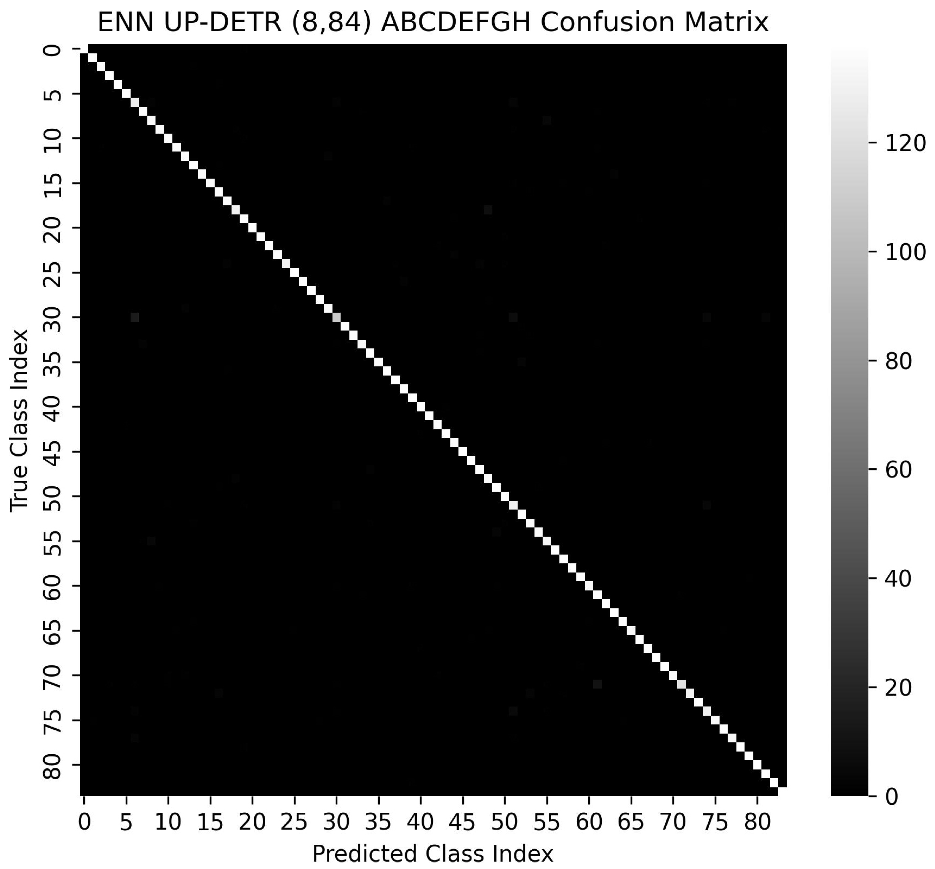
Table 11 shows the precision, recall and F1-score of one of the largest ENN model ((8,84) ABCDEFGH) using various backbone models. UP-DETR was the best performer, while Yolo showed the lowest accuracy. Figure 8 shows the confusion matrix of (8,84) ABCDEFGH model using UD-DETR. The Top-1 accuracy of this model was 98.275%.

The accuracy saturation of the single neural network model is inevitable if there are thousands of products to classify. The tipping point of the single neural network model, given much larger set of design rights, is a subject for subsequent studies. But, note that it is highly costly and time-consuming to obtain the photos of proprietary products following the design rights. Also, cooperation from the design right owner is needed to take the images of their products in various settings. Addressing the issues with data acquisition is another research topic to be studied in the future.

5. Conclusion

We presented a scalable two-stage hierarchical ensemble neural network (ENN) model tuned for detecting the design rights a product is potentially infringing. We assumed a counterfeit is merely an identical copy of the existing product with a registered design right. We identify the violated design rights by classifying the image of a product shot under different settings such as lighting, packaging condition, focal length, and angles. This study is keen on the fact that thousands of design rights are registered, and many products pour into the market at the border. Classifying a product into the thousands of design rights with a single neural network is impractical due to heavy training costs and inefficient compute resource utilization. The ENN model is designed to address the scalability issue by having distributed backbone models trained on a unit-sized dataset independently and in parallel. The result of the backbone models is concatenated and passed through the ensemble DNN model that consists of fully connected residual blocks to output the model that returned the most similar class of a given product image.

This novel structure could train the ENN model on incrementally added unit-sized datasets with constant time. Therefore, the ENN model can scale to classify many design rights. The ENN model was designed to enhance scalability. However, the fine-tuned ENN model using UP-DETR as a backbone model showed Top-1 and Top-3 accuracies of 98.27% and 99.25%, respectively. Thus, we showed that the ENN model can be on par with the single neural network model while having at least an order of magnitude lower training cost when given an incremental dataset to learn.

The ENN model is the most appropriate neural network structure to adopt in the field, with thousands of products to examine. Customizing the ENN model is easy as we can plugin any neural network model in the backbone layer for further improvement in terms of accuracy. To build a product-level design right classification system, we need to amass much larger images of real products, let alone actual illegal replicas. However, obtaining pictures of these real products under various settings is costly and time-consuming. An efficient data acquisition method for building the production-level design right classification is a subject for future work.

Author Contributions

Conceptualization, Y.Y; methodology, C.J.L, S.H.J, and Y.Y.; software, C.J.L and S.H.J,; validation, C.J.L, S.H.J, and Y.Y..; formal analysis, C.J.L, S.H.J, and Y.Y.; investigation, C.J.L, S.H.J, and Y.Y.; resources, Y.Y.; data curation, C.J.L, S.H.J, and Y.Y.; writing—original draft preparation, C.J.L, S.H.J, and Y.Y.; writing—review and editing, Y.Y.; visualization, C.J.L; supervision, Y.Y.; project administration, Y.Y.; funding acquisition, Y.Y. All authors have read and agreed to the published version of the manuscript.

Funding

This research was supported by the Ministry of Trade, Industry & Energy (MOTIE) and the Korea Institute for Advancement of Technology (KIAT), under Grants P0014268 Smart HVAC demonstration support. This research was also supported by the MSIT (Ministry of Sciencd and ICT), Korea under the ITRC (Information Technology Research Center) support program (RS-2023-00259099) supervised by the IITP (Institute for Information & Communications Technology Planning & Evaluation, and supported by the National Research Foundation of Korea(NRF) grant funded by the Korea government(MSIT) (No. RS-2023-00240211).

Abbreviations

The following abbreviations are used in this manuscript:

ENN	Ensemble Neural Network
DNN	Deep Neural Network

References

de coopération et de développement économiques, O. Trade in counterfeit and pirated goods: Mapping the economic impact; OECD Publishing, 2016.
Vaswani, A.; Shazeer, N.; Parmar, N.; Uszkoreit, J.; Jones, L.; Gomez, A.N.; Kaiser. Ł.; Polosukhin, I. Attention is all you need. Advances in neural information processing systems 2017, 30. [Google Scholar]
Kang, M.; Lee, W.; Hwang, K.; Yoon, Y. Vision transformer for detecting critical situations and extracting functional scenario for automated vehicle safety assessment. Sustainability 2022, 14, 9680. [Google Scholar] [CrossRef]
Hwang, H.; Oh, J.; Lee, K.H.; Cha, J.H.; Choi, E.; Yoon, Y.; Hwang, J.H. Synergistic approach to quantifying information on a crack-based network in loess/water material composites using deep learning and network science. Computational Materials Science 2019, 166, 240–250. [Google Scholar] [CrossRef]
Hwang, H.; Choi, S.M.; Oh, J.; Bae, S.M.; Lee, J.H.; Ahn, J.P.; Lee, J.O.; An, K.S.; Yoon, Y.; Hwang, J.H. Integrated application of semantic segmentation-assisted deep learning to quantitative multi-phased microstructural analysis in composite materials: Case study of cathode composite materials of solid oxide fuel cells. Journal of Power Sources 2020, 471, 228458. [Google Scholar] [CrossRef]
Kumar, S.N.; Singal, G.; Sirikonda, S.; Nethravathi, R. A novel approach for detection of counterfeit Indian currency notes using deep convolutional neural network. IOP Conference Series: Materials Science and Engineering. IOP Publishing, 2020, Vol. 981, p. 022018.
Lee, S.H.; Lee, H.Y. Counterfeit bill detection algorithm using deep learning. Int. J. Appl. Eng. Res 2018, 13, 304–310. [Google Scholar]
Daoud, E.; Vu, D.; Nguyen, H.; Gaedke, M. ENHANCING FAKE PRODUCT DETECTION USING DEEP LEARNING OBJECT DETECTION MODELS. IADIS International Journal on Computer Science & Information Systems 2020, 15. [Google Scholar]
Hawkins, J. A thousand brains: A new theory of intelligence; Hachette UK, 2021.
Mountcastle, V.B. Modality and topographic properties of single neurons of cat’s somatic sensory cortex. Journal of neurophysiology 1957, 20, 408–434. [Google Scholar] [CrossRef] [PubMed]
Wimmer, H.; Yoon, V.Y. Counterfeit product detection: Bridging the gap between design science and behavioral science in information systems research. Decision Support Systems 2017, 104, 1–12. [Google Scholar] [CrossRef]
He, K.; Zhang, X.; Ren, S.; Sun, J. Deep residual learning for image recognition. Proceedings of the IEEE conference on computer vision and pattern recognition, 2016, pp. 770–778.
Bochkovskiy, A.; Wang, C.Y.; Liao, H.Y.M. Yolov4: Optimal speed and accuracy of object detection. arXiv preprint arXiv:2004.10934 2020. arXiv:2004.10934 2020.
Carion, N.; Massa, F.; Synnaeve, G.; Usunier, N.; Kirillov, A.; Zagoruyko, S. End-to-end object detection with transformers. European conference on computer vision. Springer, 2020, pp. 213–229.
Dai, Z.; Cai, B.; Lin, Y.; Chen, J. Up-detr: Unsupervised pre-training for object detection with transformers. Proceedings of the IEEE/CVF Conference on Computer Vision and Pattern Recognition, 2021, pp. 1601–1610.
Torrey, L.; Shavlik, J. Transfer learning. In Handbook of research on machine learning applications and trends: algorithms, methods, and techniques; IGI global, 2010; pp. 242–264.
Yousefnezhad, M.; Hamidzadeh, J.; Aliannejadi, M. Ensemble classification for intrusion detection via feature extraction based on deep Learning. Soft Computing 2021, 25, 12667–12683. [Google Scholar] [CrossRef]
Ahn, H.; Son, S.; Kim, H.; Lee, S.; Chung, Y.; Park, D. EnsemblePigDet: Ensemble Deep Learning for Accurate Pig Detection. Applied Sciences 2021, 11, 5577. [Google Scholar] [CrossRef]
Usman, S.M.; Khalid, S.; Bashir, S. A deep learning based ensemble learning method for epileptic seizure prediction. Computers in Biology and Medicine 2021, 136, 104710. [Google Scholar]
Parhami, B. Voting algorithms. IEEE transactions on reliability 1994, 43, 617–629. [Google Scholar] [CrossRef]
Breiman, L. Bagging predictors. Machine learning 1996, 24, 123–140. [Google Scholar] [CrossRef]
Freund, Y.; Schapire, R.E.; others. Experiments with a new boosting algorithm. icml. Citeseer, 1996, Vol. 96, pp. 148–156.
Divina, F.; Gilson, A.; Goméz-Vela, F.; García Torres, M.; Torres, J.F. Stacking ensemble learning for short-term electricity consumption forecasting. Energies 2018, 11, 949. [Google Scholar] [CrossRef]
Sikora, R.; others. A modified stacking ensemble machine learning algorithm using genetic algorithms. In Handbook of research on organizational transformations through big data analytics; IGi Global, 2015; pp. 43–53.
Dou, J.; Yunus, A.P.; Bui, D.T.; Merghadi, A.; Sahana, M.; Zhu, Z.; Chen, C.W.; Han, Z.; Pham, B.T. Improved landslide assessment using support vector machine with bagging, boosting, and stacking ensemble machine learning framework in a mountainous watershed, Japan. Landslides 2020, 17, 641–658. [Google Scholar] [CrossRef]
Zagoruyko, S.; Komodakis, N. Wide residual networks. arXiv preprint arXiv:1605.07146 2016.
Tan, M.; Le, Q. Efficientnet: Rethinking model scaling for convolutional neural networks. International conference on machine learning. PMLR, 2019, pp. 6105–6114.
Van Dyk, D.A.; Meng, X.L. The art of data augmentation. Journal of Computational and Graphical Statistics 2001, 10, 1–50. [Google Scholar] [CrossRef]
Shorten, C.; Khoshgoftaar, T.M. A survey on image data augmentation for deep learning. Journal of big data 2019, 6, 1–48. [Google Scholar] [CrossRef]
Zhong, Z.; Zheng, L.; Kang, G.; Li, S.; Yang, Y. Random erasing data augmentation. Proceedings of the AAAI conference on artificial intelligence, 2020, Vol. 34, pp. 13001–13008.
Liu, Z.; Lin, Y.; Cao, Y.; Hu, H.; Wei, Y.; Zhang, Z.; Lin, S.; Guo, B. Swin transformer: Hierarchical vision transformer using shifted windows. Proceedings of the IEEE/CVF International Conference on Computer Vision, 2021, pp. 10012–10022.
Konar, J.; Khandelwal, P.; Tripathi, R. Comparison of various learning rate scheduling techniques on convolutional neural network. 2020 IEEE International Students’ Conference on Electrical, Electronics and Computer Science (SCEECS). IEEE, 2020, pp. 1–5.
Tieleman, T.; Hinton, G. Lecture 6.5-rmsprop, coursera: Neural networks for machine learning. University of Toronto, Technical Report 2012, 6. [Google Scholar]
Cherry, J.M.; Adler, C.; Ball, C.; Chervitz, S.A.; Dwight, S.S.; Hester, E.T.; Jia, Y.; Juvik, G.; Roe, T.; Schroeder, M.; others. SGD: Saccharomyces genome database. Nucleic acids research 1998, 26, 73–79. [Google Scholar] [CrossRef] [PubMed]
Kingma, D.P.; Ba, J. Adam: A method for stochastic optimization. arXiv preprint arXiv:1412.6980 2014.
Loshchilov, I.; Hutter, F. Decoupled weight decay regularization. arXiv preprint arXiv:1711.05101 2017.

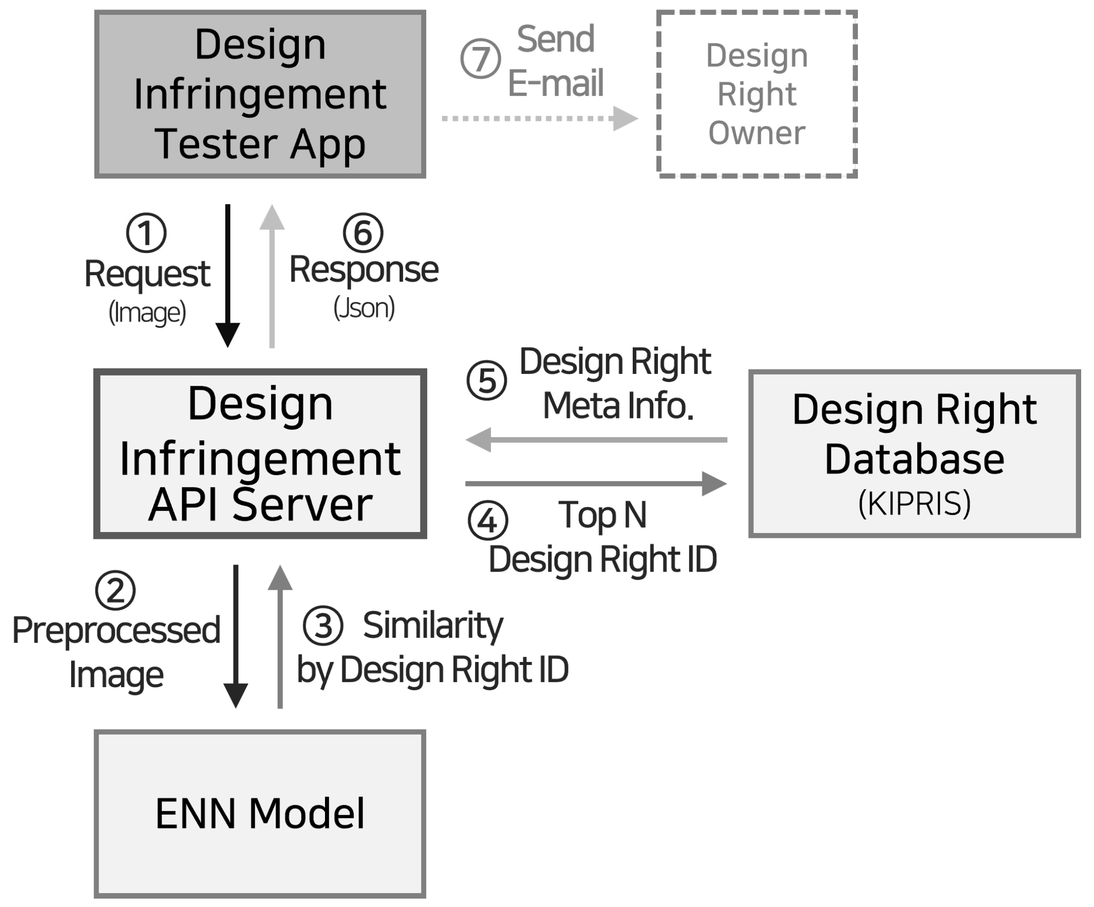
Figure 1. The overall structure of an automated system for examining counterfeit products.

Figure 2. Comparison of the structure of the previous model and ENN model. N: Total number of design rights. M : Number of sub models. C : Number of design rights on each model. K : Number of additional design rights.

Figure 3. Comparison of the structure of the previous model and ENN model when additional training is needed.

Figure 4. Structure of the DNN ensemble model.

Figure 5. An example of overlay function operation

Figure 6. This is a photo of an image being taken on a turntable for image collection. (Blurred due to copyright issues.)

Figure 7. Top-1 and Top-3 accuracy of ENN model with varying number of distributed backbone models and total number number classes. Yolo not shown here performed the worst. Accuracy of Yolo is shown in Table 4

Figure 8. Confusion matrix of (8,84) ABCDEFGH using UP-DETR

Table 1. Design rights used for the experiment

Registration Number	Product Type	International Classification	Models Applied
3008346600000	Wireless Earphones	14-03	(1,11)A, (1,21)I, (1,42)M, (1,84)O
3009240880000	Earphones	14-01	(1,11)A, (1,21)I, (1,42)M, (1,84)O
3011022290000	Earphones	14-03	(1,11)A, (1,21)I, (1,42)M, (1,84)O
3010963450000	Smartwatch	10-02	(1,11)A, (1,21)I, (1,42)M, (1,84)O
3009682050000	Auxiliary Battery for Charging Electronic Devices	13-02	(1,11)A, (1,21)I, (1,42)M, (1,84)O
3009953020000	Charger for Electronic Devices	13-02	(1,11)A, (1,21)I, (1,42)M, (1,84)O
3009911250000	Nail Clippers	28-03	(1,11)A, (1,21)I, (1,42)M, (1,84)O
3005785260000	Nail Polishing File	28-03	(1,11)A, (1,21)I, (1,42)M, (1,84)O
3009277950000	Hairdressing Scissors	28-03	(1,11)A, (1,21)I, (1,42)M, (1,84)O
3008580740000	Toner Cartridge	14-02	(1,11)A, (1,21)I, (1,42)M, (1,84)O
3010820300000	Hair Styler	28-03	(1,11)A, (1,21)I, (1,42)M, (1,84)O
3009462960000	Nail Cleaning Tool Case	03-01	(1,10)B, (1,21)I, (1,42)M, (1,84)O
3010448610000	Skin Care Machine	24-01	(1,10)B, (1,21)I, (1,42)M, (1,84)O
3009901080000	Eyeliner Container	28-02	(1,10)B, (1,21)I, (1,42)M, (1,84)O
3009727970000	Hair Dryer	28-03	(1,10)B, (1,21)I, (1,42)M, (1,84)O
3009201910000	Lipstick	28-02	(1,10)B, (1,21)I, (1,42)M, (1,84)O
3008635170000	Hair Dryer	28-03	(1,10)B, (1,21)I, (1,42)M, (1,84)O
3006924410000	Front Bumper Cover for Car	12-16	(1,10)B, (1,21)I, (1,42)M, (1,84)O
3005781700000	Cartridge for Printer Developer	14-02	(1,10)B, (1,21)I, (1,42)M, (1,84)O
3009950260000	Nail Clippers	28-03	(1,10)B, (1,21)I, (1,42)M, (1,84)O
3005904250000	Packaging Container	09-01	(1,10)B, (1,21)I, (1,42)M, (1,84)O
3007711150000	Humidifier	23-04	(1,11)C, (1,21)J, (1,42)M, (1,84)O
3008140280000	Spray Container for Cosmetic Packaging	09-01	(1,11)C, (1,21)J, (1,42)M, (1,84)O
3005222300000	Cosmetic Containers	09-01	(1,11)C, (1,21)J, (1,42)M, (1,84)O
3006924390000	Car Radiator Grill	12-16	(1,11)C, (1,21)J, (1,42)M, (1,84)O
3010336170000	Fan	23-04	(1,11)C, (1,21)J, (1,42)M, (1,84)O
3006037400000	Hair Dryer	28-03	(1,11)C, (1,21)J, (1,42)M, (1,84)O
3009746650000	Spray Container for Packaging	09-01	(1,11)C, (1,21)J, (1,42)M, (1,84)O
3010424520002	Portable Vacuum Cleaner	15-05	(1,11)C, (1,21)J, (1,42)M, (1,84)O
3009508860000	Skin Care Machine	28-03	(1,11)C, (1,21)J, (1,42)M, (1,84)O
3005872160000	Nail Clippers	28-03	(1,11)C, (1,21)J, (1,42)M, (1,84)O
3010277880000	Portable Air Purifier	23-04	(1,11)C, (1,21)J, (1,42)M, (1,84)O
3006394680000	Front Fog Lamp for Car	26-06	(1,10)D, (1,21)J, (1,42)M, (1,84)O
3010353420000	Stylus Pen	14-99	(1,10)D, (1,21)J, (1,42)M, (1,84)O
3008337320000	Car Head Lamp	26-06	(1,10)D, (1,21)J, (1,42)M, (1,84)O
3008337300000	Automotive Rear Combination Lamp	26-06	(1,10)D, (1,21)J, (1,42)M, (1,84)O
3008486220000	Front Bumper Cover for Car	12-16	(1,10)D, (1,21)J, (1,42)M, (1,84)O
3008486270000	Car Radiator Grill	12-16	(1,10)D, (1,21)J, (1,42)M, (1,84)O
3008433850000	Car Wheel	12-16	(1,10)D, (1,21)J, (1,42)M, (1,84)O
3009369070000	Cell Phone Protection Case	03-01	(1,10)D, (1,21)J, (1,42)M, (1,84)O
3009505900000	Infant Head Protector	02-99	(1,10)D, (1,21)J, (1,42)M, (1,84)O
3006471740000	Heat Therapy Device	24-01	(1,10)D, (1,21)J, (1,42)M, (1,84)O
3020200055040	Wireless Earphones	14-03	(1,11)E, (1,21)K, (1,42)N, (1,84)O
3008488090000	Infant Head Protector	02-99	(1,11)E, (1,21)K, (1,42)N, (1,84)O
3007512050000	Animal Toys	21-01	(1,11)E, (1,21)K, (1,42)N, (1,84)O
3007827830000	Vacuum Cleaner	15-05	(1,11)E, (1,21)K, (1,42)N, (1,84)O
3010328940000	Hairdressing Scissors	28-03	(1,11)E, (1,21)K, (1,42)N, (1,84)O
3006880340000	Car Head Lamp	26-06	(1,11)E, (1,21)K, (1,42)N, (1,84)O
3006314510000	Developer for Printer	14-02	(1,11)E, (1,21)K, (1,42)N, (1,84)O
3005792510000	Hair Dryer	28-03	(1,11)E, (1,21)K, (1,42)N, (1,84)O

Table 2. Design rights used for the experiment

Registration Number	Product Type	International Classification	Models Applied
3009137110000	Robotic Vacuum	15-05	(1,11)E, (1,21)K, (1,42)N, (1,84)O
3005633730000	Nail Clippers	28-03	(1,11)E, (1,21)K, (1,42)N, (1,84)O
3006880350000	Automotive Rear Combination Lamp	26-06	(1,11)E, (1,21)K, (1,42)N, (1,84)O
3007892610000	Hair Dryer	28-03	(1,10)F, (1,21)K, (1,42)N, (1,84)O
3004925580000	Hair Dryer	28-03	(1,10)F, (1,21)K, (1,42)N, (1,84)O
3009277940000	Hairdressing Scissors	28-03	(1,10)F, (1,21)K, (1,42)N, (1,84)O
3009664240000	Infant Head Protector	02-03	(1,10)F, (1,21)K, (1,42)N, (1,84)O
3010776320000	Cheering Equipment	21-03	(1,10)F, (1,21)K, (1,42)N, (1,84)O
3007488730000	Nail Clippers	28-03	(1,10)F, (1,21)K, (1,42)N, (1,84)O
3006812870000	Doll	21-01	(1,10)F, (1,21)K, (1,42)N, (1,84)O
3005777720000	Electric Hair Straightener	28-03	(1,10)F, (1,21)K, (1,42)N, (1,84)O
3008380770000	General Beauty Scissors	08-03	(1,10)F, (1,21)K, (1,42)N, (1,84)O
3006813180000	Hair Brush	04-02	(1,10)F, (1,21)K, (1,42)N, (1,84)O
3007298000000	Electric Hair Straightener	28-03	(1,11)G, (1,21)L, (1,42)N, (1,84)O
3009442540000	Nail Clippers with Magnifying Glass Attached	28-03	(1,11)G, (1,21)L, (1,42)N, (1,84)O
3010468310000	Head Guard	02-99	(1,11)G, (1,21)L, (1,42)N, (1,84)O
3007845090000	Stationery Scissors	08-03	(1,11)G, (1,21)L, (1,42)N, (1,84)O
3006955750000	Doll	21-01	(1,11)G, (1,21)L, (1,42)N, (1,84)O
3008976800000	Cheering Tool	21-03	(1,11)G, (1,21)L, (1,42)N, (1,84)O
3009317560000	Doll	21-01	(1,11)G, (1,21)L, (1,42)N, (1,84)O
3011212930000	Cheering Tool	21-03	(1,11)G, (1,21)L, (1,42)N, (1,84)O
3008380780000	Beauty Thinning Scissors	08-03	(1,11)G, (1,21)L, (1,42)N, (1,84)O
3009052330000	Hair Dryer	28-03	(1,11)G, (1,21)L, (1,42)N, (1,84)O
3011182010000	Infant Head Protection	02-03	(1,11)G, (1,21)L, (1,42)N, (1,84)O
3005633760000	Nail Clippers	28-03	(1,10)H, (1,21)L, (1,42)N, (1,84)O
3010696720000	Cheering Equipment	21-03	(1,10)H, (1,21)L, (1,42)N, (1,84)O
3007449670000	Hair Brush	04-02	(1,10)H, (1,21)L, (1,42)N, (1,84)O
3010123750000	Nail Clippers	28-03	(1,10)H, (1,21)L, (1,42)N, (1,84)O
3011236760000	Cheering Light Stick	21-03	(1,10)H, (1,21)L, (1,42)N, (1,84)O
3009505920000	Infant Head Protector	02-99	(1,10)H, (1,21)L, (1,42)N, (1,84)O
3005480740000	Hand Puppet	21-01	(1,10)H, (1,21)L, (1,42)N, (1,84)O
3011211790000	Cheering Tool	21-03	(1,10)H, (1,21)L, (1,42)N, (1,84)O
3008039980000	Hair Styler	28-03	(1,10)H, (1,21)L, (1,42)N, (1,84)O
3007797260000	Cheering Glow Stick	21-03	(1,10)H, (1,21)L, (1,42)N, (1,84)O

Table 3. Average UP-DETR training time per epoch with varying number of design rights.

Num of Design Rights	10	11	14	21	42	84
Average Train Time per Epoch ( $m i n$ )	3.0	3.5	4.5	6.75	15.25	29.5

Table 4. Average Top-1 and Top-3 accuracy(%) of individual backbone models. Model is distinguished in a tuple followed by a letter ID. The first and the second elements of the tuple are the number of backbone models and the number of design rights learned, respectively. The letter ID indicates a group of design rights.

Model	UP-DETR		Yolo		EfficientNet		ResNet		WideResNet
	Top-1	Top-3	Top-1	Top-3	Top-1	Top-3	Top-1	Top-3	Top-1	Top-3
(1,11) A	99.868	100.000	96.443	97.958	99.868	100.000	99.671	100.000	98.090	99.868
(1,10) B	100.000	100.000	95.072	97.681	99.710	100.000	99.783	100.000	99.348	100.000
(1,11) C	99.934	100.000	93.478	97.826	99.802	100.000	99.407	100.000	99.275	100.000
(1,10) D	100.000	100.000	90.290	96.232	99.783	100.000	98.333	99.855	99.565	99.855
(1,11) E	100.000	100.000	94.137	97.167	99.473	100.000	99.605	100.000	98.353	99.934
(1,10) F	99.928	100.000	95.000	98.333	99.855	100.000	99.203	100.000	97.754	100.000
(1,11) G	99.868	100.000	96.509	99.012	100.000	100.000	99.868	100.000	99.539	100.000
(1,10) H	100.000	100.000	96.957	98.043	99.783	100.000	98.551	100.000	97.826	100.000
(1,21) I	99.896	100.000	96.653	97.964	99.862	100.000	99.517	99.965	99.517	99.931
(1,21) J	100.000	100.000	97.861	98.896	99.896	100.000	99.551	100.000	99.655	99.965
(1,21) K	99.965	100.000	96.308	98.689	99.931	100.000	99.068	100.000	99.482	99.965
(1,21) L	100.000	100.000	98.344	99.413	99.655	100.000	99.310	100.000	98.965	100.000
(1,42) M	99.879	100.000	97.981	98.689	99.948	100.000	99.586	100.000	99.620	100.000
(1,42) N	99.845	100.000	96.411	99.051	99.931	100.000	99.396	99.983	99.396	99.983
(1,84) O [Single]	99.784	99.957	90.709	96.299	99.905	100.000	99.569	99.983	99.681	99.983

Table 5. Top-1 and Top-3 accuracy(%) of the ENN model with varying layer size. The letter IDs identify the group of design rights. For example, (2,21)AB means that 42 design rights are divided into groups ’A’ and ’B’.

Model	2048		1024		512		256
	Top-1	Top-3	Top-1	Top-3	Top-1	Top-3	Top-1	Top-3
(2,21) AB	98.861	99.827	98.930	99.966	98.689	99.827	98.930	99.827
(3,32) ABC	98.483	99.502	98.256	99.592	98.120	99.457	98.211	99.389
(4,42) ABCD	98.585	99.500	98.344	99.362	98.568	99.431	98.413	99.465
(5,53) ABCDE	97.963	99.330	98.154	99.289	98.031	99.180	97.744	99.180
(6,63) ABCDEF	98.068	99.160	98.321	99.149	98.033	99.103	98.137	99.275
(7,74) ABCDEFG	98.051	99.158	98.296	99.315	98.267	99.119	98.228	99.128
(8,84) ABCDEFGH	98.361	99.163	98.318	99.198	98.137	99.129	98.102	99.180
Average	98.339	99.377	98.374	99.410	98.264	99.321	98.252	99.349

Table 6. Accuracy(%) of the ENN model according to the dropout rate.

Model	0.1		0.2		0.3		0.4		0.5
	Top-1	Top-3	Top-1	Top-3	Top-1	Top-3	Top-1	Top-3	Top-1	Top-3
(2,21) AB	98.965	99.896	98.930	99.966	98.723	99.827	98.999	99.896	98.965	99.793
(3,32) ABC	98.188	99.547	98.256	99.592	98.279	99.547	98.392	99.660	98.256	99.479
(4,42) ABCD	98.551	99.517	98.344	99.362	98.620	99.517	98.447	99.500	98.326	99.413
(5,53) ABCDE	97.935	99.221	98.154	99.289	97.935	99.262	98.113	99.439	98.195	99.330
(6,63) ABCDEF	98.068	99.034	98.321	99.149	97.930	99.045	98.263	99.218	98.091	99.114
(7,74) ABCDEFG	98.237	99.285	98.296	99.315	98.208	99.138	98.374	99.256	98.159	99.138
(8,84) ABCDEFGH	98.206	99.111	98.318	99.198	98.456	99.172	98.275	99.249	98.068	99.189
Average	98.307	99.373	98.374	99.410	98.307	99.358	98.409	99.460	98.294	99.351

Table 7. Accuracy(%) of the ENN model according to the learning rate.

Model	0.05		0.01		0.005		0.001
	Top-1	Top-3	Top-1	Top-3	Top-1	Top-3	Top-1	Top-3
(2,21) AB	98.689	99.827	98.689	99.793	98.999	99.896	98.758	99.827
(3,32) ABC	97.917	99.774	97.962	99.592	98.392	99.660	98.053	99.457
(4,42) ABCD	97.912	99.465	98.378	99.569	98.447	99.500	98.223	99.362
(5,53) ABCDE	96.874	98.742	97.635	99.166	98.113	99.439	97.949	99.262
(6,63) ABCDEF	97.239	99.275	98.022	99.137	98.263	99.218	98.079	99.160
(7,74) ABCDEFG	97.131	99.158	98.149	99.266	98.374	99.256	98.306	99.275
(8,84) ABCDEFGH	97.041	99.120	98.223	99.224	98.275	99.249	98.352	99.180
Average	97.543	99.337	98.151	99.392	98.409	99.460	98.246	99.360

Table 8. Accuracy(%) of the ENN model according to the optimizer.

Model	AdamW		Adam		SGD		RMSprop
	Top-1	Top-3	Top-1	Top-3	Top-1	Top-3	Top-1	Top-3
(2,21) AB	98.999	99.896	98.792	99.896	98.413	99.758	95.169	99.965
(3,32) ABC	98.392	99.660	98.324	99.615	97.962	99.706	92.278	99.841
(4,42) ABCD	98.447	99.500	98.671	99.465	98.447	99.655	85.059	99.638
(5,53) ABCDE	98.113	99.439	98.141	99.330	97.676	99.398	80.476	99.316
(6,63) ABCDEF	98.263	99.218	98.091	99.137	97.930	99.275	76.398	98.884
(7,74) ABCDEFG	98.374	99.256	98.365	99.138	98.188	99.226	72.111	98.570
(8,84) ABCDEFGH	98.275	99.249	98.378	99.146	98.240	99.180	69.117	97.559
Average	98.409	99.460	98.395	99.390	98.122	99.457	81.515	99.111

Table 9. Accuracy(%) of the ENN model according to the depth of FC residual block depth.

Model	4		5		6		7		8
	Top-1	Top-3	Top-1	Top-3	Top-1	Top-3	Top-1	Top-3	Top-1	Top-3
(2,21) AB	98.930	99.896	99.034	99.862	98.999	99.896	98.896	99.655	98.896	99.827
(3,32) ABC	98.370	99.502	98.370	99.592	98.392	99.660	98.211	99.298	98.211	99.434
(4,42) ABCD	98.447	99.551	98.568	99.500	98.447	99.500	98.464	99.603	98.413	99.482
(5,53) ABCDE	98.059	99.385	98.045	99.371	98.113	99.439	97.799	99.330	98.195	99.412
(6,63) ABCDEF	98.447	99.195	98.114	99.126	98.263	99.218	98.022	99.195	98.298	99.264
(7,74) ABCDEFG	97.993	99.128	98.159	99.266	98.374	99.256	98.208	99.187	98.296	99.226
(8,84) ABCDEFGH	98.240	99.258	98.223	99.198	98.275	99.249	98.275	99.224	98.413	99.224
Average	98.355	99.417	98.359	99.416	98.409	99.460	98.268	99.356	98.389	99.410

Table 10. Comparison of accuracy(%) according to the number of model separations.

Model	UP-DETR		Yolo		EfficientNet		ResNet		WideResNet
	Top-1	Top-3	Top-1	Top-3	Top-1	Top-3	Top-1	Top-3	Top-1	Top-3
(2,21) AB	98.930	99.896	90.683	96.756	96.687	99.965	96.515	99.965	94.237	99.482
(3,32) ABC	98.370	99.502	87.228	95.267	96.445	99.728	95.245	99.343	93.524	98.777
(4,42) ABCD	98.447	99.551	84.972	93.099	96.377	99.551	94.910	98.982	93.841	98.602
(5,53) ABCDE	98.059	99.385	83.443	92.508	94.750	99.152	94.217	98.728	92.931	98.496
(6,63) ABCDEF	98.447	99.195	83.506	91.534	95.480	98.930	94.134	98.401	93.214	98.217
(7,74) ABCDEFG	97.993	99.128	83.500	91.324	95.554	98.796	94.036	98.110	93.400	97.983
(8,84) ABCDEFGH	98.275	99.249	83.791	91.442	95.980	98.896	94.229	98.137	93.599	97.800
(4,84) IJKL	98.878	99.672	88.708	96.368	95.385	99.603	95.057	99.094	93.703	98.913
(2,84) MN	98.404	99.189	93.444	98.490	96.946	99.965	96.912	99.784	96.006	99.862
(1,84) O	99.784	99.957	90.709	96.299	99.905	100.000	99.569	99.983	99.681	99.983

Table 11. Precision, Recall, and F1 Score of one of the largest model, (8,84) ABCDEFGH

Model	Precision	Recall	F1 Score
UP-DETR	98.309	98.275	98.271
Yolo	84.267	83.791	83.718
EfficientNet	96.019	95.980	95.961
ResNet	94.284	94.229	94.212
WideResNet	93.690	93.599	93.593

Short Biography of Authors

	Chan Jae Lee received a bachelor’s degree in urban engineering from Hongik University in 2019 and a master’s degree in Artificial Intelligence and Big Data in the Industrial Convergence Interdepartmental Program in 2021. From 2021, he has been an Artificial Intelligence Researcher in the Future Technology Strategy Lab of NetcoreTech. His research interests include Machine Learning, Deep Learning, Big Data, Computer Vision, Large Graph, and Smart City.
	Seong Ho Jeong received a bachelor’s degree in Mathematics from Incheon National University in 2021. From 2021, he has been an Artificial Intelligence Researcher in the Future Technology Strategy Lab of NetcoreTech. His research interests include Machine Learning, Deep Learning, Big Data, and Computer Vision.
	Young Yoon received a bachelor’s degree and master’s degree in Computer Sciences from the University of Texas at Austin in 2003 and 2006, respectively. He also earned his doctoral’s degree in Computer Engineering from University of Toronto in 2013. From 2015, he has been an assistant professor in the Department of Computer Science at Hongik University. His research interests include distributed computing, middleware, and applied artificial intelligence.

Disclaimer/Publisher’s Note: The statements, opinions and data contained in all publications are solely those of the individual author(s) and contributor(s) and not of MDPI and/or the editor(s). MDPI and/or the editor(s) disclaim responsibility for any injury to people or property resulting from any ideas, methods, instructions or products referred to in the content.

© 2023 by the authors. Licensee MDPI, Basel, Switzerland. This article is an open access article distributed under the terms and conditions of the Creative Commons Attribution (CC BY) license (http://creativecommons.org/licenses/by/4.0/).

Copyright: This open access article is published under a Creative Commons CC BY 4.0 license, which permit the free download, distribution, and reuse, provided that the author and preprint are cited in any reuse.

MDPI Initiatives

Important Links

Choose an area of interest and we will send you notifications of new preprints at your preferred frequency.

Disclaimer

ENN: Hierarchical Image Classification Ensemble Neural Network for Large-Scale Automated Detection of Potential Design Infringement

Abstract

1. Introduction

2. Related Works

3. Methodology

3.1. Model architecture

3.1.1. The distributed backbone model

3.1.2. The Ensemble DNN model

4. Experiments

4.1. Experiment setup and implementation

4.2. Data collection and augmentation

4.3. Comparison of training speed

4.4. Comparison of distributed backbone models

4.5. Hyper-parameter tuning

4.6. Comparison with a single network model

5. Conclusion

Author Contributions

Funding

Abbreviations

References

Short Biography of Authors

MDPI Initiatives

Important Links

Subscribe