1. Introduction
Building Energy Management System (BEMS) covers the entire electricity system, from power generation to consumption, including generation, transmission, distribution, and consumption. Energy management software, implemented in areas with high energy usage such as households, buildings, and factories, analyzes energy consumption to determine whether energy is being consumed appropriately by energy source, heat source, system, and major equipment. The goal is to establish an efficient energy management system, leading to cost savings from energy conservation, reviewing appropriate energy usage of energy sources, reducing carbon emissions through optimal operation, decreasing facility operation and maintenance costs, extending equipment lifespan, and improving facility operation efficiency, all of which contribute to increased building value [
1,
2].
Despite the numerous advantages of BEMS, reliable forecasting of electricity consumed in buildings is essential. Electricity consumption forecasting can be categorized into very short-term, short-term, medium-term, and long-term forecasts [
3,
4,
5]. Very-short term electricity consumption forecasting predicts power consumption and demand in real time by performing predictions for 1 hour, 15 min, and 30 min to stably operate power. Short-term electricity consumption forecasting covers predictions ranging from hourly to a few weeks using algorithms such as Exponential Smoothing [
6] and Auto Regressive Integrated Moving Averages (ARIMA) [
7]. Conversely, medium-term electricity consumption forecasting spans a few weeks to several months and utilizes various variables such as meteorological data, event information, and economic indicators to predict power consumption. Different algorithms such as linear regression, multiple regression, polynomial regression [
8], neural networks [
9], deep learning [
10], and Long Short-term Memory (LSTM) [
11] are used. Long-term electricity consumption forecasting involves predictions spanning three months to a year, and it requires consideration of more variables and system elements than short-term and medium-term forecasts. Time series analysis, ARIMA models, and ensemble techniques can help predict the trends and patterns of long-term power consumption.
ARIMA is effective for short-term forecasts but challenging to apply to data with seasonality or non-stationarity, and it struggles to predict long-term patterns. Exponential Smoothing is useful for short-term forecasting but faces challenges in predicting long-term trends and incorporating other factors. The Prophet is suitable for medium-term forecasting and can handle seasonality and events, but it struggles to predict long-term trends. LSTM is suitable for long-term forecasting as it learns long-term dependencies in time series data, but it is sensitive to the quantity and quality of data and requires significant computational resources for training and prediction [
12,
13,
14].
Recent electricity consumption forecasting algorithms combine various techniques based on data characteristics and forecasting objectives [
15,
16,
17,
18,
19,
20]. For example, combining Prophet and LSTM shows improved accuracy and performance in short-term and long-term electricity consumption predictions [
15,
16]. Other studies propose combining ARIMA and XGBoost for short-term electricity consumption forecasting [
17] and ARIMA and Bi-LSTM models for smart grid parameters [
18]. Additionally, a combination of ARIMA-LSTM and ARIMA-GRU models uses ARIMA to model trends and seasonality in time series data and LSTM to improve prediction performance [
19,
20]. The previously mentioned studies have evaluated the strengths, weaknesses, and performance of the models, thereby establishing criteria for model selection. However, the complexity of parameter configuration and the training process associated with the combination of these two models can be intricate. Furthermore, the performance may vary based on the application domain, as well as the characteristics of the data.
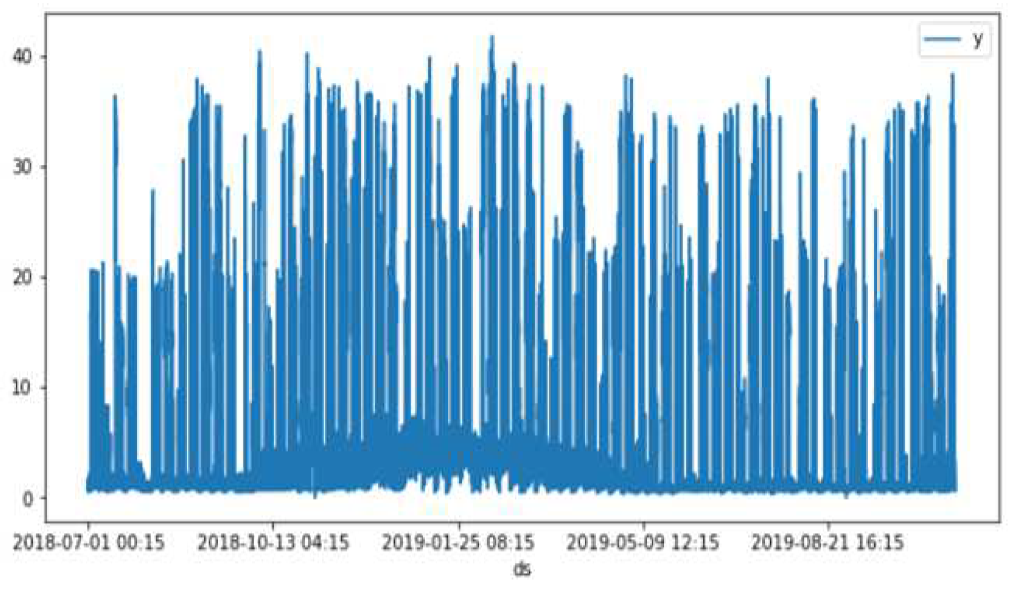
This study proposes a method for short- and medium-term electricity consumption prediction by combining the GRU model, suitable for long-term forecasting, and the Prophet model, suitable for capturing seasonality and events. In this study, simulation data collected from July 1, 2018, to October 31, 2019, in 15-minute intervals represents the electricity consumption of Company B in Naju, Jeollanam-do. Meteorological data is collected hourly from a weather observation point closest to Naju, Gwangju.
The proposed methodology is as follows:
(1) Collect and preprocess electricity consumption data and meteorological data.
(2) Utilize the preprocessed data to propose the Prophet model in the first step for handling seasonality and events.
(3) In the second step, simulate seven multivariate datasets, consisting of six meteorological data variables and observed electricity consumption data, using the GRU model.
(4) Predict electricity consumption at 15-minute intervals using the residuals between the data predicted by the proposed Prophet model in Step 1 and the observed data, along with the six meteorological data variables.
(5) Conduct experiments for short-term (2 days and 7 days) and medium-term (15 days and 30 days) electricity consumption predictions.
The study's structure is as follows:
Section 2 discusses related research on the Prophet and GRU models.
Section 3 addresses the problems of the existing Prophet and proposes solutions.
Section 4 explains the algorithm and experimental results of the proposed method. Finally,
Section 5 concludes the study.
4. Proposed methods
The flow chart of the proposed method in this study is shown in
Figure 7.
Section 4.1 explains how to collect data,
Section 4.2 describes the pre-processing method for collected data,
Section 4.3 describes how to divide data for learning and testing,
Section 4.4 describes the proposed method using prophet and GRU, and finally, the study concludes with error measurements and visualizations.
4.1. Data collection
In this study, the electricity consumption data used is collected from a company, B Corporation (machinery manufacturing), located in Naju, Jeollanam-do, South Korea. The data spans from July 1, 2018, to October 31, 2019, with a time interval of 15 minutes.
To enhance the accuracy of electricity consumption predictions, various factors, including Korean holidays (alternative holidays, election days, national holidays, etc.), are taken into account. The Workalendar package is utilized to generate the Korean holiday data. Additionally, meteorological data such as temperature, precipitation, wind speed, humidity, sunshine duration, and cloud cover are collected at hourly intervals from the Korea Meteorological Administration's weather data portal (
http://www.weather.go.kr).
4.2. Data pre-processing
The meteorological data is then resampled using linear interpolation to match the 15-minute intervals of the electricity consumption data. To handle missing values in both power and meteorological data, they are filled with zeros. To minimize the impact of outliers, the
RobustScaler method [
23] is applied to normalize the data scale, as shown in equation (3).
In equation (3), is the scaled data, is the original data, Q1(x) is the first quartile of the data, and Q3(x) is the third quartile of the data. By using RobustScaler, we ensure that the data is normalized while being less sensitive to the influence of outliers.
4.3. Data partition for training and test data
The training data spans from July 1, 2018, to June 31, 2019, and the test data covers the period from July 1, 2019, to October 31, 2019. The data is split into a 75% portion for training and a 25% portion for testing to conduct the experiments.
4.4. Proposed prophet model
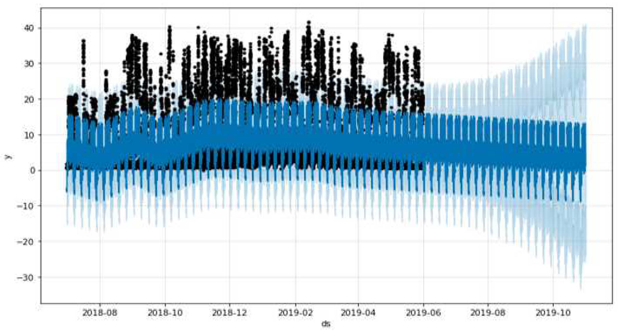
The experimental training data used in this study consists of electricity consumption data collected from July 2018 to May 2019. The modified Prophet model was simulated with components including trends, seasonality, holidays, flows, and others, as outlined in
Table 1. Notably, the
'df' variable in the holiday parameters was adjusted to account for substitute holidays in this study. Both regular holidays and substitute holidays, such as election days and traditional holidays, within this time frame were taken into consideration to enhance the accuracy of electricity consumption predictions.
In this study, the correlation coefficient was used as shown in Equation (4) to evaluate the accuracy of the long-term and short-term predictions [
24].
In Equation (4), and represent the mean of X and Y, respectively, and and represent the standard deviation of X and Y, respectively, while n represents the number of data points.
For long-term predictions (1-year period) and short-term predictions (2 days), the correlation coefficients between the predicted electricity consumption and the observed consumption were found to be 0.67 and 0.87, respectively. This indicates that the modified Prophet model performs poorly for long-term electricity consumption predictions. However, the correlation coefficient of 0.87 for short-term predictions indicates that the model performs better than for long-term predictions. Therefore, the proposed Prophet model was used for short-term electricity consumption predictions.
4.5. Proposed GRU model
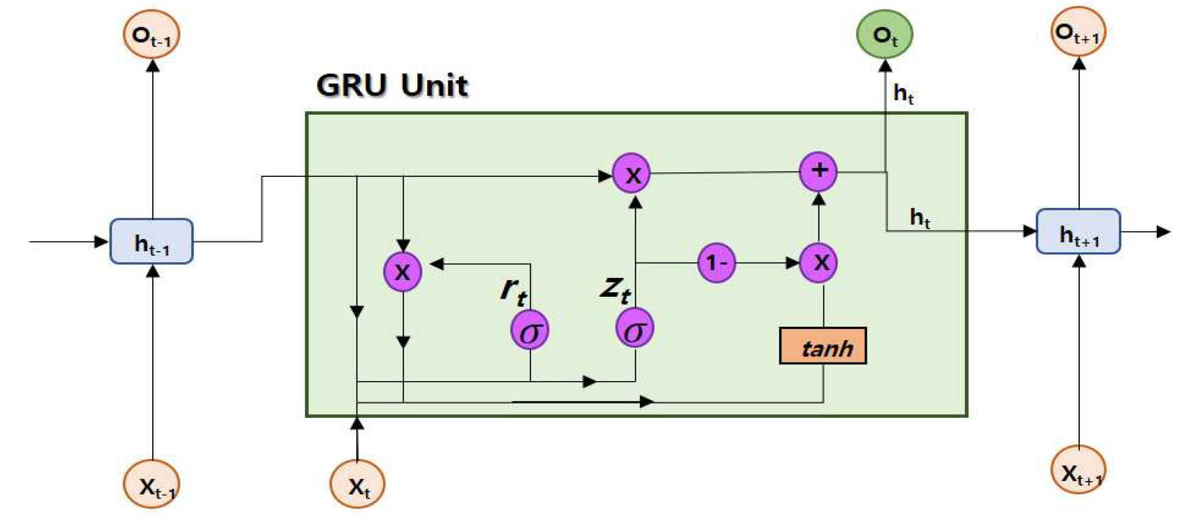
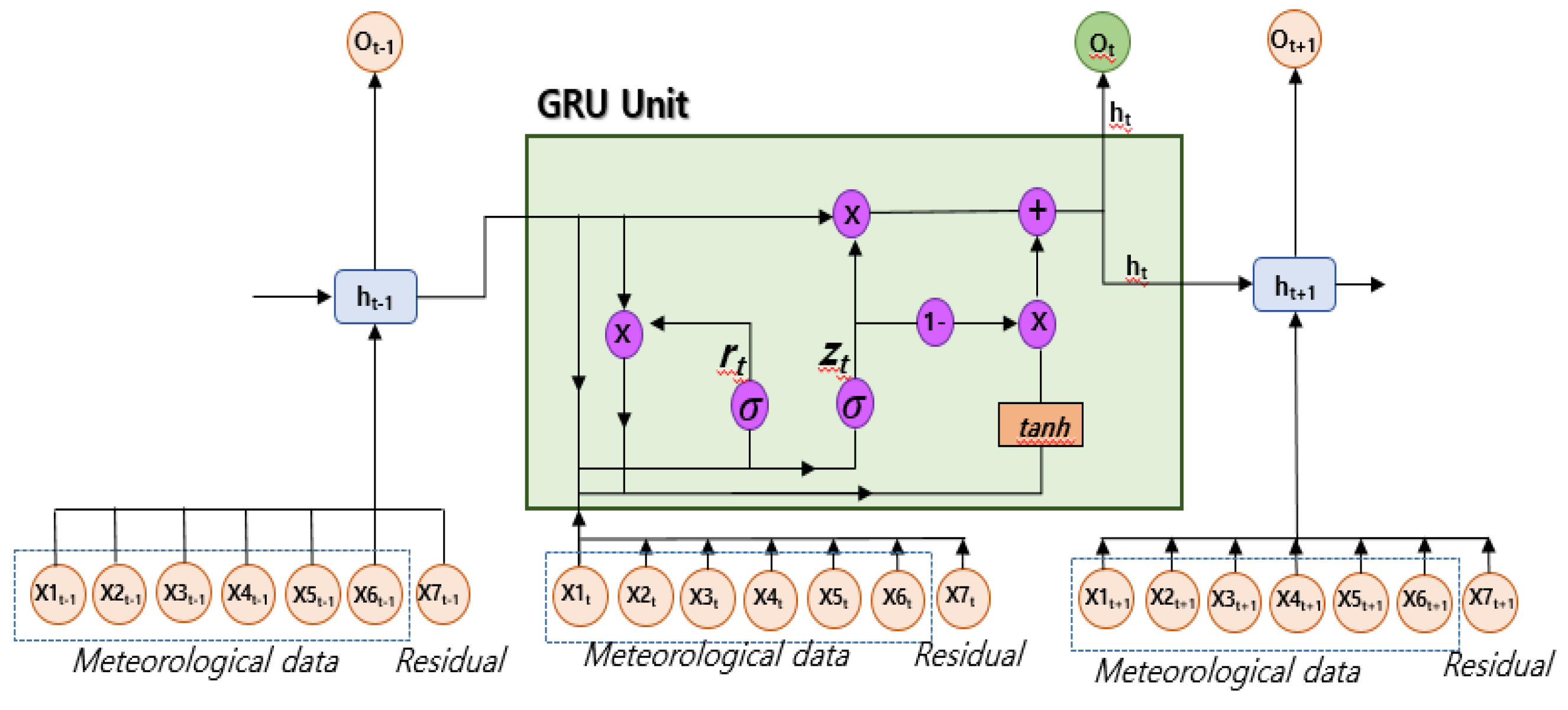
To reduce the errors between Prophet's predictions and observed values, we propose incorporating GRU, as shown in
Figure 10. Among various meteorological data that influence electricity consumption forecasting, the study adopted and utilized the six (temperature, precipitation, wind speed, humidity, sunshine duration, and cloud cover) most impactful variables for this study [
25]. The input data consists of multiple variables, including meteorological data (temperature, precipitation, wind speed, humidity, sunshine duration, and cloud cover) and the residual (the difference between the predictions and observed values obtained from the Prophet model in the first step), totaling 7 variables.
In
Figure 10,
to
represent the meteorological data from the previous time point (
t-1), i.e., temperature, precipitation, wind speed, humidity, sunshine duration, and cloud cover.
represents the residual. The traditional GRU prediction model typically targets the entire consumption data for electricity consumption predictions. However, in this study, we apply the residuals of the long-term trend (yearly and monthly) predictions to the GRU model, as shown in Equation (5), to predict electricity consumption and reduce error rates.
In Equation (5), "Residual" denotes the residual, "Prophetpred" represents the predictions obtained from the original Prophet model, and "y" is the observed consumption value. The GRU model's training and validation data are derived from the same dataset. The input layer of the GRU model consists of 7 variables, which include 6 meteorological data variables (temperature, precipitation, wind speed, humidity, sunshine duration, cloud cover), and 1 residual variable. The hidden layer of the GRU model contains 7 nodes. The initial learning rate is set to 0.005, and the maximum number of iterations is 50,000. The mean square error (MSE) is used as the loss function, and the ADAM optimizer (Adaptive Moment Estimation) is employed during training and testing.
6. Conclusion
The electricity consumption forecasting is crucial in the electricity industry and energy system operations as it helps improve efficiency and stability. It provides valuable information to energy companies, power suppliers, network operators, and other stakeholders involved in energy management. This study proposes a short- and medium-term forecasting algorithm, combining the Prophet and GRU models, for predicting building electricity consumption over 2 days, 7 days, 15 days, and 30 days. The proposed method outperforms both the modified Prophet and GRU using multivariate.
Our proposed method offers a versatile and effective solution for optimizing energy management within Building Energy Management Systems, with the potential for substantial cost savings, improved energy source utilization, reduced carbon emissions, and enhanced operational efficiency, ultimately increasing the overall value of the building.
Figure 1.
Electricity consumption data of Company B collected from July 1, 2018, to October 31, 2019.
Figure 1.
Electricity consumption data of Company B collected from July 1, 2018, to October 31, 2019.
Figure 2.
A basic Prophet model that only considers the holiday effect on the training data for one year (July 2018 to June 2019).
Figure 2.
A basic Prophet model that only considers the holiday effect on the training data for one year (July 2018 to June 2019).
Figure 3.
Trend, holidays, weekly, and daily prediction analysis of basic prophet model. The blue line shows the trend the model fits from the test data, and the light blue shade shows the predicted trend.
Figure 3.
Trend, holidays, weekly, and daily prediction analysis of basic prophet model. The blue line shows the trend the model fits from the test data, and the light blue shade shows the predicted trend.
Figure 5.
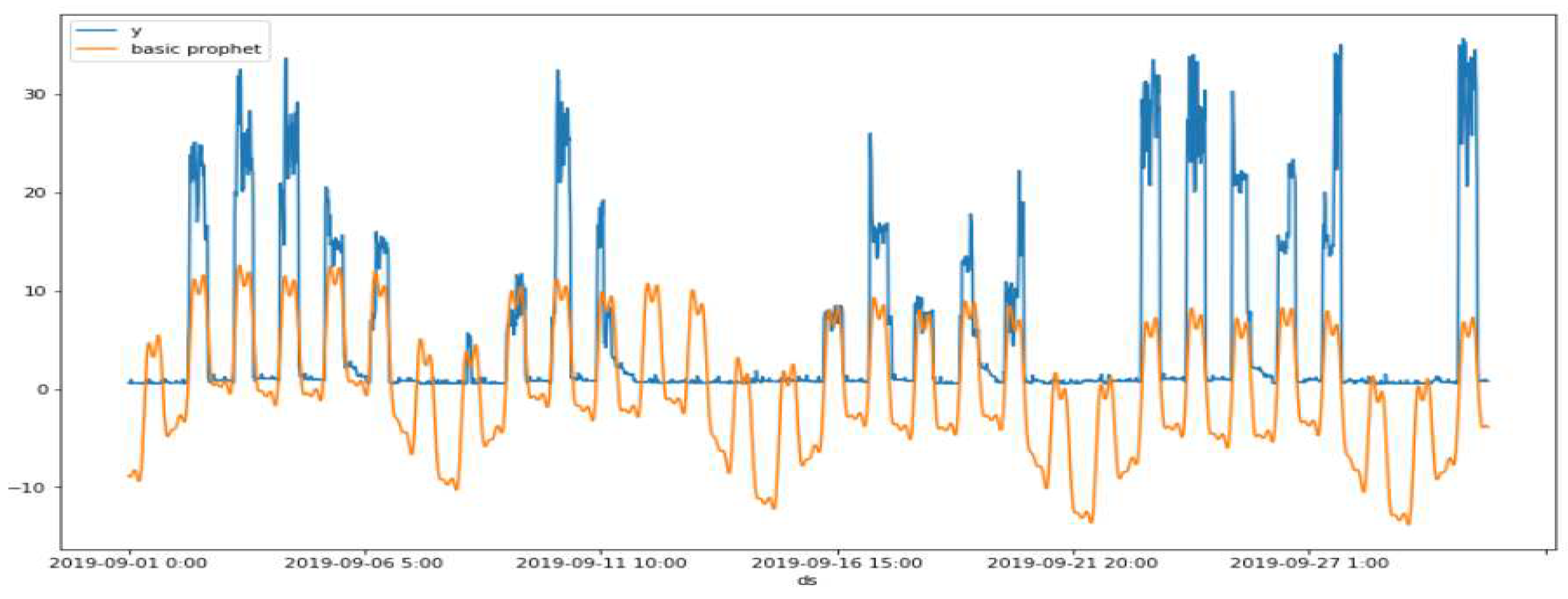
Performance comparison between observed value (y) and basic prophet model (basic prophet) from July 1st to 30th, 2019.
Figure 5.
Performance comparison between observed value (y) and basic prophet model (basic prophet) from July 1st to 30th, 2019.
Figure 6.
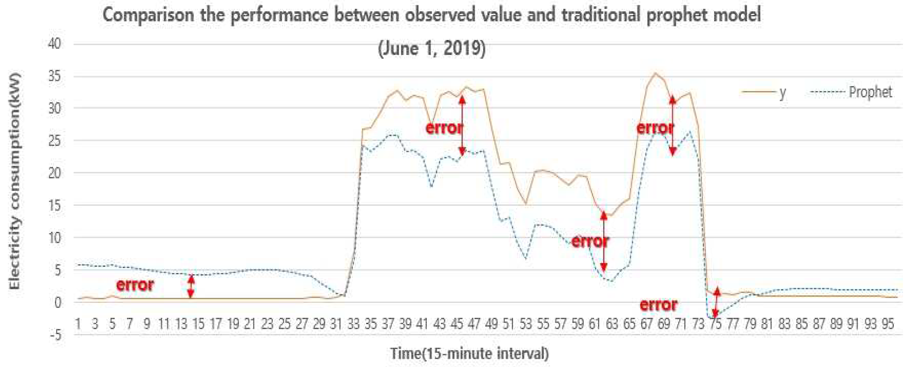
Performance comparison between the observed value (y) and the basic prophet model’s value (Prophet) on July 1st, 2019.
Figure 6.
Performance comparison between the observed value (y) and the basic prophet model’s value (Prophet) on July 1st, 2019.
Figure 7.
The flowchart of the proposed method.
Figure 7.
The flowchart of the proposed method.
Figure 8.
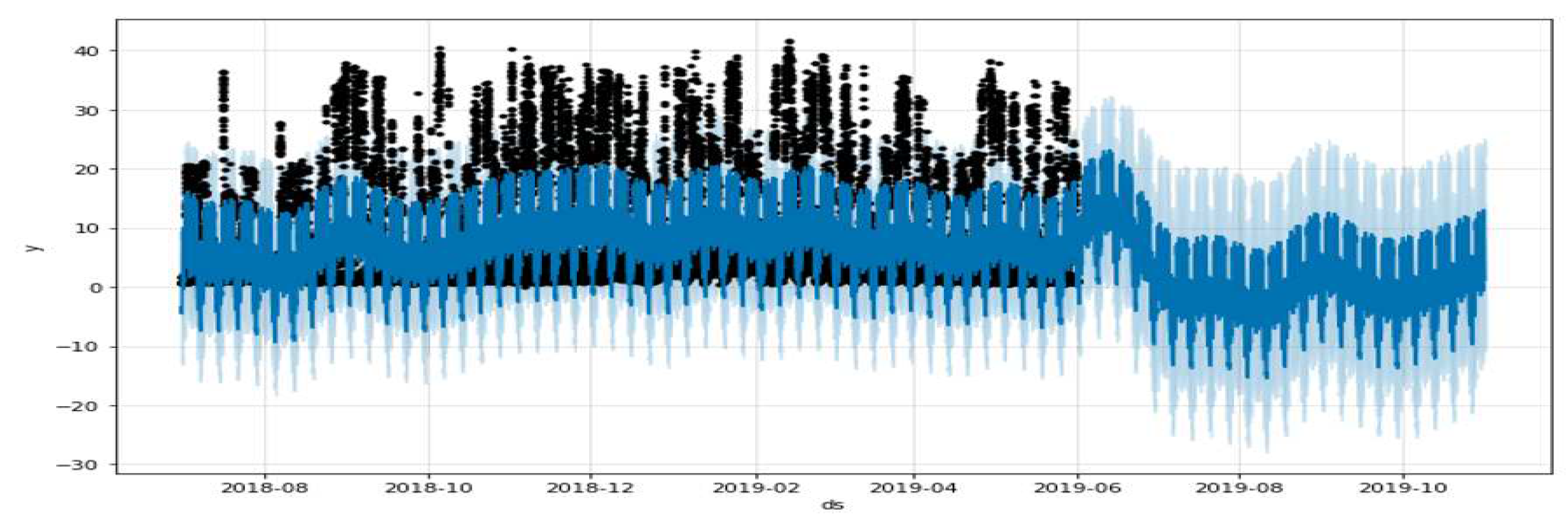
Error forecast of the proposed Prophet model. The black dots represent the historical input data, the blue line represents the predicted trend line after model fitting, and the light blue area above and below the blue curve represents the confidence interval.
Figure 8.
Error forecast of the proposed Prophet model. The black dots represent the historical input data, the blue line represents the predicted trend line after model fitting, and the light blue area above and below the blue curve represents the confidence interval.
Figure 9.
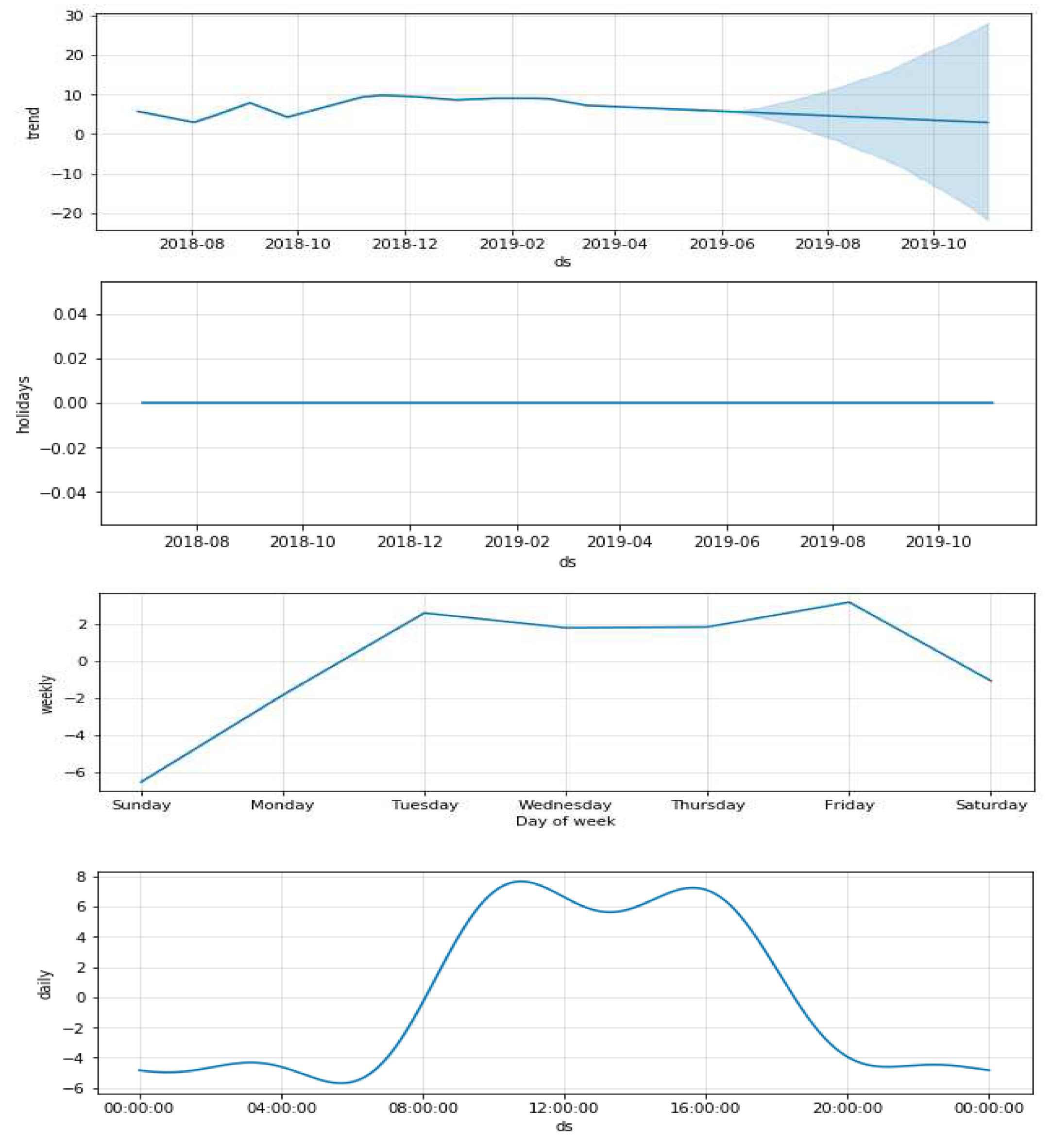
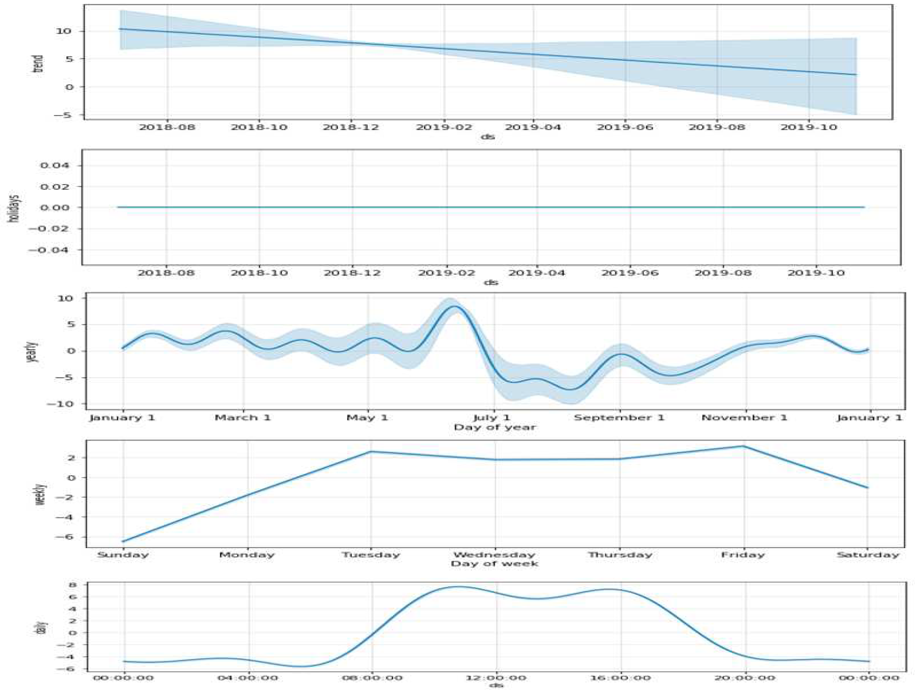
Trend, holidays, weekly, and daily prediction analysis of the proposed prophet model. The blue line shows the trend the model fits from the test data, and the light blue shade shows the predicted trend.
Figure 9.
Trend, holidays, weekly, and daily prediction analysis of the proposed prophet model. The blue line shows the trend the model fits from the test data, and the light blue shade shows the predicted trend.
Figure 10.
Structure of proposed GRU model.
Figure 10.
Structure of proposed GRU model.
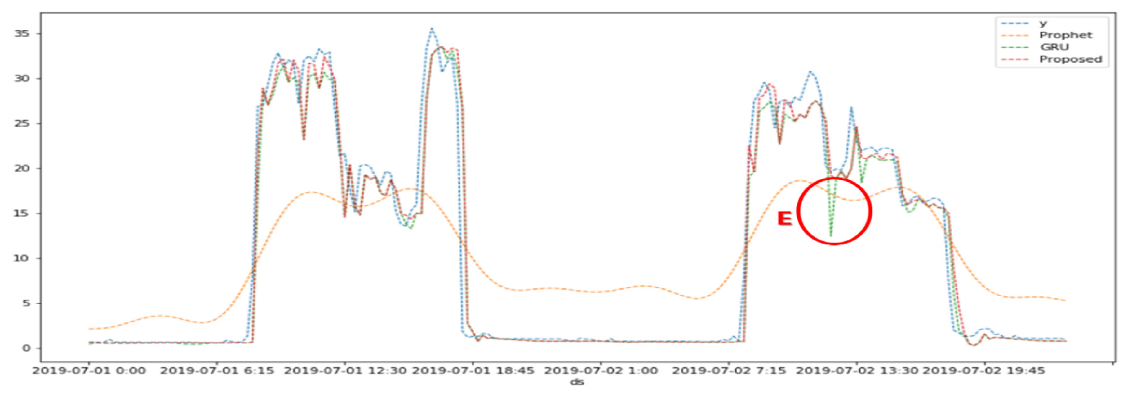
Figure 11.
Comparison of graphic visualization performance between observed values (y) and other methods (modified Prophet, GRU using multivariate, and Propose) from July 1 to July 2, 2019.
Figure 11.
Comparison of graphic visualization performance between observed values (y) and other methods (modified Prophet, GRU using multivariate, and Propose) from July 1 to July 2, 2019.
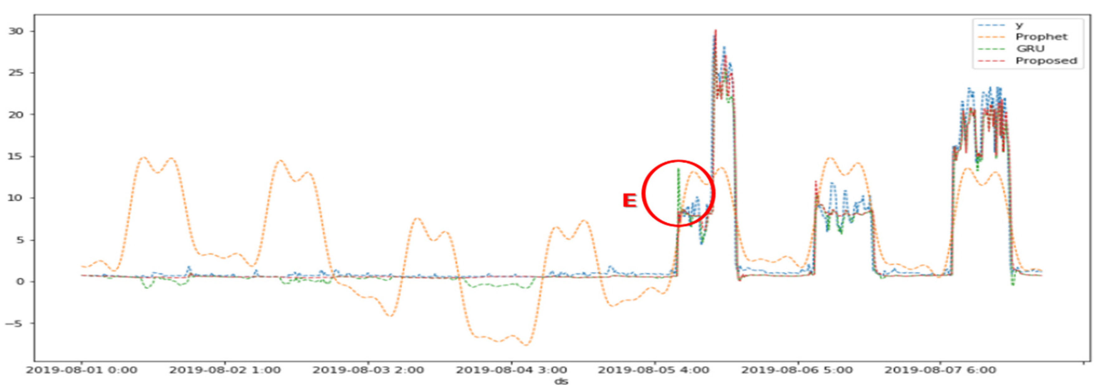
Figure 12.
Comparison of graphic visualization performance between observed values (y) and other methods (modified Prophet, GRU using multivariate, and Propose) from Aug. 1 to Aug. 7, 2019.
Figure 12.
Comparison of graphic visualization performance between observed values (y) and other methods (modified Prophet, GRU using multivariate, and Propose) from Aug. 1 to Aug. 7, 2019.
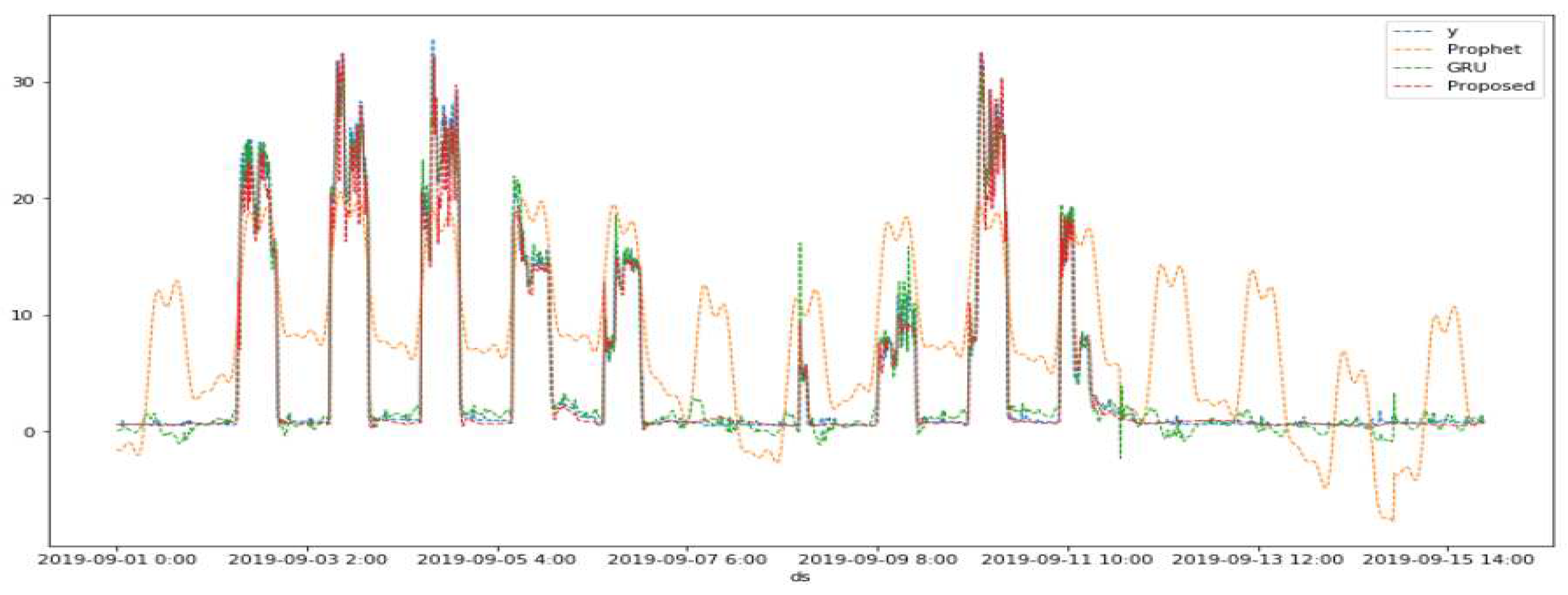
Figure 13.
Comparison of graphic visualization performance between observed values (y) and other methods (modified Prophet, GRU using multivariate, and Propose) from Sep. 1 to Sep. 15, 2019.
Figure 13.
Comparison of graphic visualization performance between observed values (y) and other methods (modified Prophet, GRU using multivariate, and Propose) from Sep. 1 to Sep. 15, 2019.
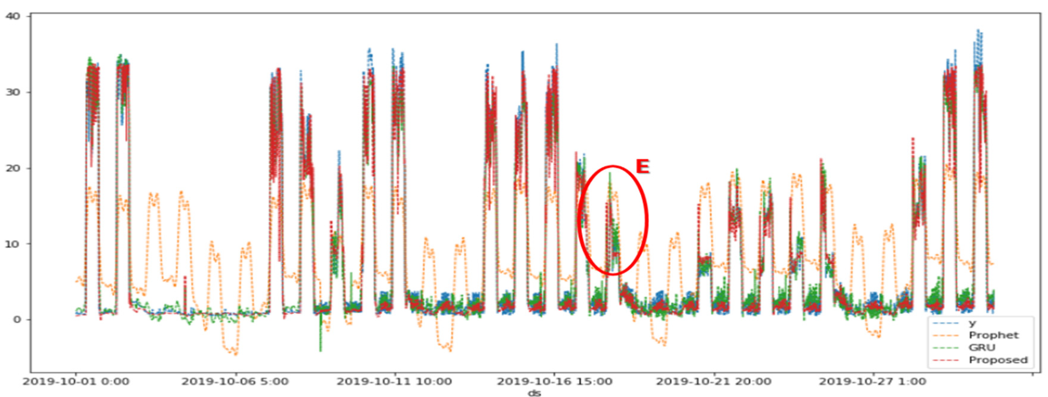
Figure 14.
Comparison of graphic visualization performance between observed values (y) and other methods (modified Prophet, GRU using multivariate, and Propose) from Oct. 1 to Oct. 30, 2019.
Figure 14.
Comparison of graphic visualization performance between observed values (y) and other methods (modified Prophet, GRU using multivariate, and Propose) from Oct. 1 to Oct. 30, 2019.
Table 1.
Proposed prophet model parameter setting.
Table 1.
Proposed prophet model parameter setting.
| Parameter Nature |
Parameter Name |
Value |
| Trend Parameters |
growth |
linear |
| changepoints |
None |
| n_changepoints |
25 |
| changepoint_range |
0.8 |
| changepoint_prior_scale |
0.01 |
| Seasonality parameters |
yearly_seasonality |
10 |
| weekly_seasonality |
False |
| daily_seasonality |
False |
| seasonality_mode |
multiplicative |
| seasonality_prior_scale |
10 |
| Holidays parameters |
holidays
Holidays_prior_scale
|
df
0.25
|
| Flow parameters |
flow |
flow |
| flow_prior_scale |
10 |
| Other parameters |
mcmc_samples |
0 |
| interval_width |
0.8 |
Table 2.
Comparison of the performance of modified Prophet, GRU, and proposed method.
Table 2.
Comparison of the performance of modified Prophet, GRU, and proposed method.
| Term |
Metrics |
Prophet |
GRU |
Proposed |
Short-
term |
2 days
(July 1~2) |
CC |
0.88 |
0.97 |
0.97 |
| MAPE (%) |
316.56 |
25.09 |
24.57 |
| SMAPE (%) |
97.58 |
20.53 |
19.72 |
7 days
(Aug. 1~7) |
CC |
0.51 |
0.97 |
0.98 |
| MAPE (%) |
526.62 |
48.07 |
27.32 |
| SMAPE (%) |
123.01 |
59.07 |
30.09 |
Medium-
term |
15 days
( Sep. 1~15) |
CC |
0.70 |
0.98 |
0.98 |
| MAPE (%) |
579.80 |
42.55 |
24.61 |
| SMAPE (%) |
125.98 |
50.76 |
22.58 |
30 days
(Oct. 1~30) |
CC |
0.67 |
0.97 |
0.98 |
| MAPE (%) |
348.06 |
37.66 |
34.37 |
| SMAPE (%) |
103.92 |
42.48 |
33.28 |
