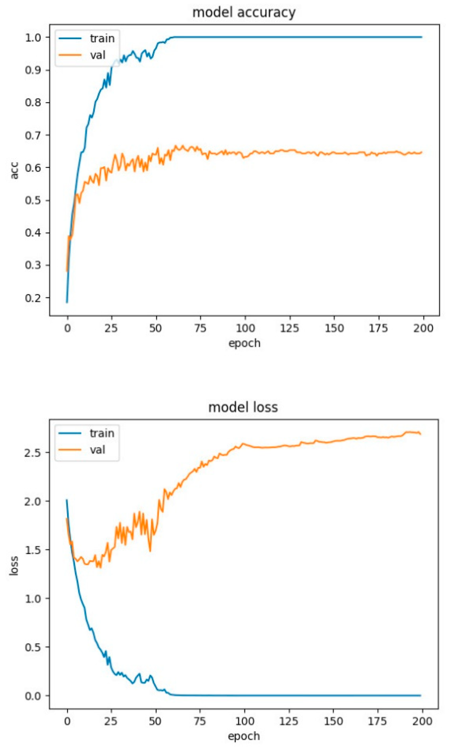
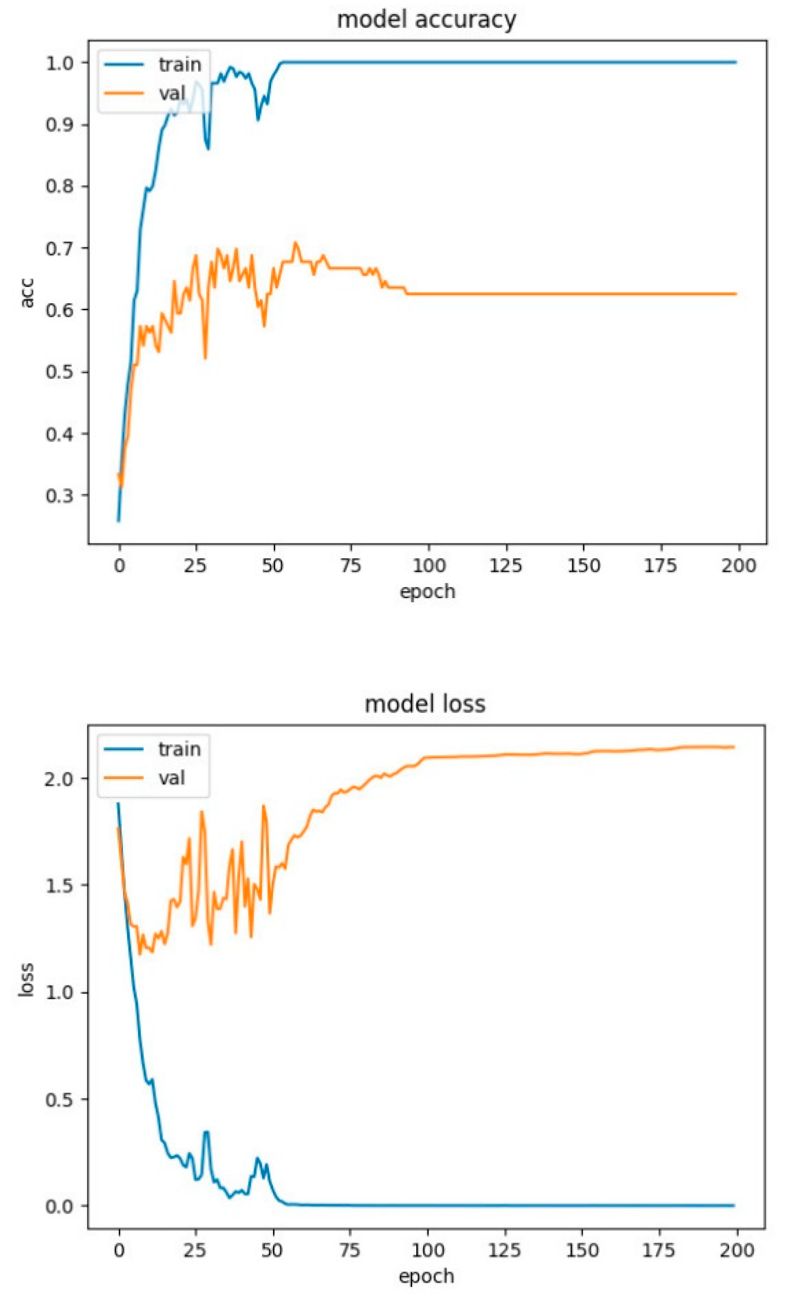
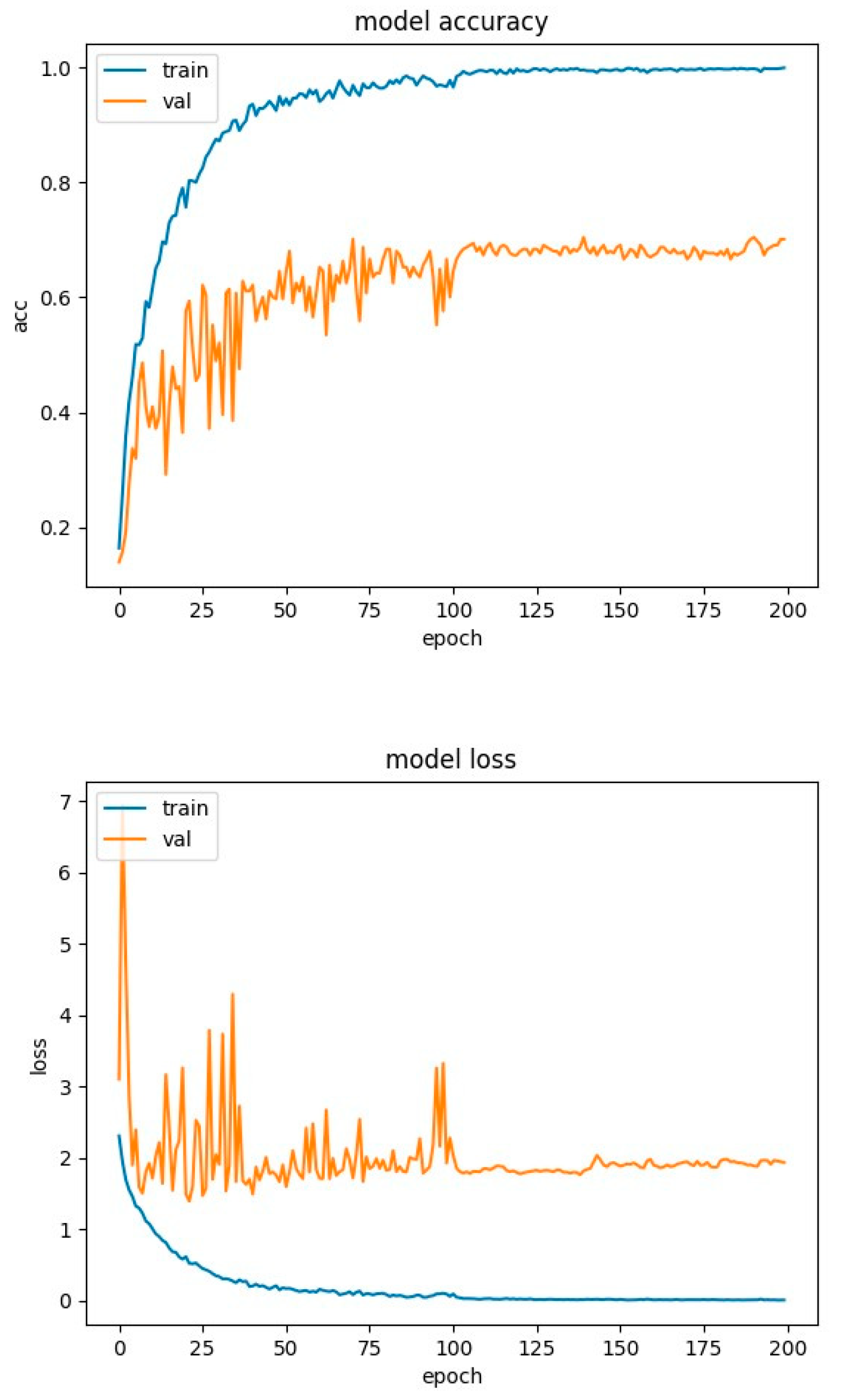
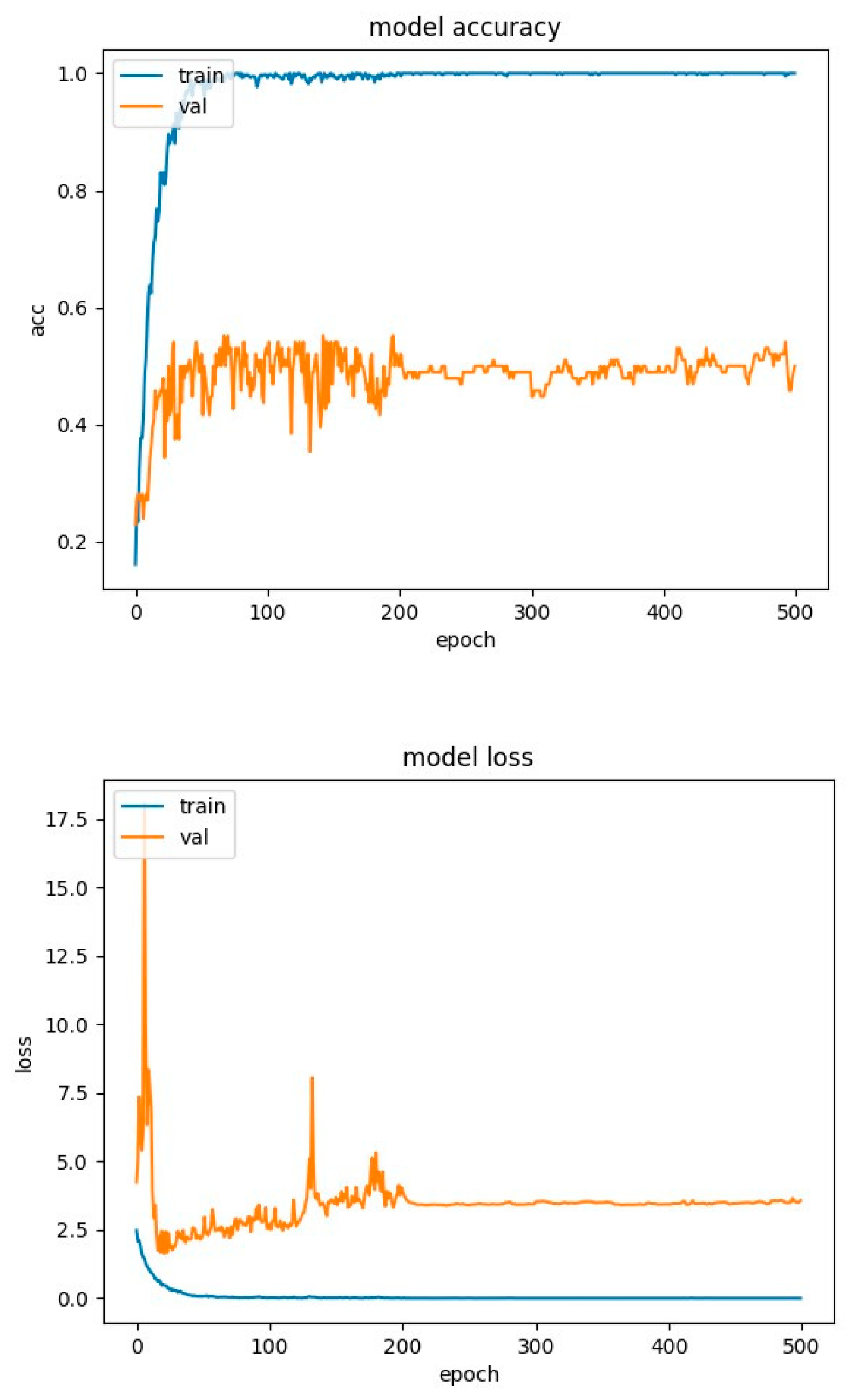
Preprint
Article

Speech Emotion Recognition Using Convolutional Neural Networks with Attention Mechanism

Altmetrics

Downloads

131

Views

43

Comments

0

A peer-reviewed article of this preprint also exists.

Submitted:

18 September 2023

Posted:

19 September 2023

You are already at the latest version

Alerts
Abstract
Speech Emotion Recognition (SER) is an interesting and difficult problem to handle. In this paper, we deal with it through the implementation of deep learning networks. We have designed and implemented six different deep learning networks, a Deep Belief Network (DBN), a simple deep neural network (SDNN), a LSTM network (LSTM), a LSTM network with the addition of an attention mechanism (LSTM-ATN), a Convolutional neural network (CNN), and a Convolutional neural network with the addition of an attention mechanism (CNN-ATN), having in mind, apart from solving the SER problem, to test the impact of attention mechanism to the results. Dropout and Batch Normalization techniques are also used to improve the generalization ability (prevention of overfitting) of the models as well as to speed up the training process. The Surrey Audio-Visual Expressed Emotion database (SAVEE), and the Ryerson Audio-Visual Database (RAVDESS) database were used for training and evaluation of our models. The results showed that networks with the addition of the attention mechanism did better than the others. Furthermore, they showed that CNN-ATN was the best among tested networks, achieving an accuracy of 74% for the SAVEE and 77% for the RAVDESS dataset, and exceeded existing state-of-the-art systems for the same datasets.
Keywords: 
Subject: Computer Science and Mathematics  -   Artificial Intelligence and Machine Learning

1. Introduction

Speech is the most natural way of human communication. Affective computing systems based on speech play an important role in promoting human-computer interaction, and emotion recognition is the first step. Due to the lack of a precise definition of emotion and the inclusive and complex influence of emotion generation and expression, accurately recognizing speech emotions is still difficult. Speech emotion recognition (SER) is an important problem, which is receiving increasing interest from researchers due to its numerous applications, such as e-learning [1], clinical trials [2], audio monitoring/surveillance, lie detection [3], entertainment, video games [4], and call centers [5]. Machine learning (ML) is a revolutionary method, in which we feed a machine an adequate amount of data and the machine will use the experience gained from the data to improve its own algorithm and process data better in the future [6]. One of the most significant approaches in machine learning is Neural Networks (NNs). NNs are networks of interconnected nodes, called neurons. NNs are loosely modeled towards the way human brain processes information. NNs store data, learn from it, and improve their abilities to sort new data. For example, a neural network having the task of identifying dogs can be fed a set of characteristic values extracted from various images of dogs tagged with the type of dog. Over time, it will learn what kind of image corresponds to what kind of dog. The machine therefore learns from experience and improves itself. Deep Learning (DL) is a recent ML approach, where NNs are arranged into sprawling networks with many layers that are trained using massive amounts of data. In DL, the sprawling artificial neural network is fed representations of raw data (e.g., raw image representations) and not given any other instructions. This means that in contrast to other ML approaches, it determines the important characteristics and purpose of the data itself, while storing it as experience. In other words, according to studies, Deep neural networks (DNNs) can solve the data representation problem through learning a series of task-specific transformations [7]. The network layers extract abstract representations and filter out the irrelevant information, which leads to a more accurate classification and better generalization. Temporal models were also proposed for modelling sequential data with mid to long-term dependencies. DL models are currently used to solve problems such as face recognition, voice recognition, image recognition, computational vision, and speech emotion recognition. One of the main advantages of DL techniques over other ML techniques is the automatic selection of features, which could, for example, be applied to important features inherent in audio files that have a special emotion in the task of recognizing speech emotions.
When it comes to recognizing emotion through speech, deep learning models such as Convolutional Neural Networks (CNN), Deep Neural Networks (DNNs), Deep Belief Networks (DBNs) etc, approach the detection of high-level features for better accuracy compared to hand-made low-level features. Furthermore, the use of deep neural networks enhances the computational complexity of the entire model. However, according to Mustaqeem and Kwon [8] there are still many challenges in recognizing emotion from speech, such as the fact that the current CNN architectures have not shown significant improvement in speech accuracy and complexity in speech signal processing, or the fact that the use of Recurrent Neural Networks (RNNs) and Long Short-Term Memory neurons (LSTMs) are useful for training sequential data, but they are difficult to train effectively and are computationally more complex. Due to the above issues and challenges, we propose a CNN architecture with the addition of an attention mechanism. The voice characteristics of the speakers are extracted in the form of Mel Frequency Cepstral Coefficients (MFCCs), with the help of the Librosa library.
The structure of the paper is as follows. Section 2 presents related work. In Section 3, six deep neural network configurations are presented. A detailed presentation of the experiments and a discussion of the proposed method compared to other research methods are provided in Sections. Finally, Section 5 concludes the paper.

2. Related Work

In the literature, there is a huge research interest, and several works attempt to perform emotion detection from speech [9,10]. DL techniques have achieved breakthrough performance in recent years, and as a result, have been thoroughly examined by the research community [11,12]. Existing studies have focused on improving and extending DL techniques.
In the work presented in [13], authors present a new Random Deep Belief Network (RDBN) method for speech emotion recognition, which consists of random subspace, DBN and SVM in the context of ensemble learning. It first extracts the low-level characteristics of the input speech signal and then applies them to the construction of many random sub-intervals. Second, it creates many different sub-intervals. In addition, DBN continues to use the stochastic gradient descent method to optimize the parameters. To solve the problem, a random space is applied for the training of the basic classifiers for the whole, where the same classification method is used. The best accuracies achieved are, 82.32% on the Emo-DB database, 48.5% on the CASIA database, 48.5% on the FAU database, and 53.60% on the SAVEE database.
In the work presented in [14], authors introduce a method for identifying speech emotions using spectrogram and a Convolutional Neural Network (CNN). The proposed model consists of three convolution layers and three fully connected layers, which extract distinctive features from spectrograph images and predictions for the seven emotions of the Emo-DB Database. Layer C1 has 120 cores (11 x 11) applied at a rate of 4 pixels. ReLU acts as an activation function instead of the standard sigmoid functions that improve the efficiency of the educational process. Layer C2 has 256 cores of size 5 x 5 and are applied to the input with one step 1. Similarly, C3 has 384 cores of size 3 x 3. Each of these convolution layers is followed by ReLUs. Layer C3 is followed by three FC layers that have 2048, 2048 and 7 neurons, respectively. More than 3000 spectrograms were generated from all the audio files in the dataset. Overall, the proposed method achieved 84.3% accuracy.
In [15], authors present two Convolutional Neural Networks with a Long-Short Memory Network (CNN-LSTM), one one-dimensional (1D) and one two-dimensional (2D), stacking four designed local features learning blocks (LFBL). The 1D CNN-LSTM network is intended to recognize the feeling of speaking from raw audio clips, while the 2D CNN-LSTM network focuses on learning high-level capabilities from log-mel spectrograms. The experimental study was conducted on Berlin Emo-DB and IEMOCAP databases. The 1D CNN LSTM network achieved 92.34% and 86.73% recognition accuracy on the speaker-dependent and speaker-independent EmoDB database respectively, and also delivered 67.92% and 79.72% recognition accuracy on the IEMOCAP dependent and independent speaker database respectively. The 2D CNN LSTM network achieved 95.33% and 95.89% recognition accuracy, on the speaker-dependent and independent speaker Emo-DB database respectively, and delivered 89.16% and 85.58% recognition accuracy on the IEMOCAP experiment database depending on the speaker and independently of the speaker respectively.
In the work presented in [16], authors proposed a new approach to the multimodal recognition of emotions from simple speech and text data. The attention network implemented consists of three separate Convolutional Neural Networks (CNNs), two for extracting features from speech spectrograms and word integration sequence, and one for the emotion classifier. The CNN outputs from word integration and spectrograms are used to calculate an attention matrix to represent the correlation between word integration and spectrogram in relation to emotion signaling. To evaluate the model, they used audio and text data from CMU-Multimodal Opinion Sentiment and Emotion Intensity (CMU-MOSEI) dataset. The dataset is organized by video IDs and corresponding segments with six emotion and sentiment labels. Video IDs are then further split into segments. The training set consisted of 3303 video ID and 23453 segments, while the validation set consisted of non- overlapping 300 video IDs and 1834 segments. The total accuracy of the proposed method was 83.11%.
In [17], authors present three methods based on CNNs in combination with extensive features, CNN + RNN and ResNet, respectively. Authors investigate different types of features as end-to-end frame input, including primary wave data, the Q-transform constant spectrogram (CQT), and the Fourier transform short-term spectrogram (STFT). In this way, authors create multiple data samples with slightly modified speed ratio, which helps them achieve significant improvements and handle the overfitting issue in the framework from end to end. For their experiments, they used the EmotAsS dataset. The CNN + RNN model achieved the best performance (45.12%) with data balancing, the CNN model in combination with features showed a performance of 34.33% with data balancing, while ResNet model achieved a 37.78% performance.
In the work presented in [18], authors propose a new architecture, called attention-based 3-Dimensional Convolutional Recurrent Neural Networks (3-D ACRNN) for recognizing emotion from speech, combining CRNN with an attention mechanism, because they hypothesized that calculating delta and delta-deltas for individual functions not only retains effective emotional information, but also reduces the effect of emotionally unrelated factors, leading to a reduction in misclassification. First, CNN 3-D is applied to the entire logarithmic-Mel spectrogram, which has been compiled into a patch that contains only multiple frames. The attention layer then takes a sequence of high-level attributes as input to generate expression-level attributes. Authors evaluated the model using the Berlin Emotional Speech Database (Emo-DB) and IEMOCAP databases. From the 10 speakers, for each evaluation they selected 8 as training data, 1 as validation and the rest as test data. The method achieved an accuracy of 64.74% on IEMOCAP and 82.82% on Emo-DB.
In the work presented in [19], authors propose an attention-pooling representation learning method for recognizing emotions from speech (SER). Emotional representation is learned from end to end by applying a Deep Convolutional Neural Network (CNN) directly to speech spectrograms extracted from speech. Compared to existing aggregation methods, such as max-pooling and average-pooling, the proposed attention pooling can effectively integrate bottom-up class-agnostic attention maps and top-down class-specific attention maps. Given an expression, they segment it into 2s sections for training and use an overlay of 1s to allow them to receive more training data. Each section corresponds to the same tag with the corresponding expression. They used a 1 × 1 convolutional layer after Conv5 to create a top-down attention map and used another 1 × 1 convolutional layer to create bottom-up attention maps. The IEMOCAP improvised dataset was used, and the accuracy achieved by the proposed method was 71.75% for WA and 68.06% for UA.
In [20], authors explore how to take full advantage of low-level and high-level audio features taken from different aspects and how to take full advantage of DNN’s ability to merge multiple information to achieve better classification performance. For this reason, they proposed a hybrid platform consisting of three units, namely, a features extraction unit, a heterogeneous unification unit and a fusion network unit. Besides low-level acoustic features, such as IS10, MFCCs and eGemaps that are extracted, high-level acoustic feature presentations named SoundNet bottleneck feature and VGGish bottleneck feature, are considered for speech emotion recognition task. The heterogeneous integration unit is a Denoising AutoEncoder (DAE), which is a multi-layer feed-forward neural network and is introduced in order to convert the heterogeneous space of various features into a unified representation space by deploying this unsupervised feature learning technique. The fusion network module is utilized to capture the associations between those unified joint features for emotion recognition task and is constructed as a four-layer neural network, containing one input layer and three hidden layers. They evaluated the model using the IEMOCAP database and the proposed method improved the recognition performance reaching an accuracy of 64%.
In the work presented in [21], authors propose a platform that at the training layer has 3 main stages, such as verbal/non-verbal audio segmentation, the integration of feature extraction and the construction of an emotion model. Verbal sections were used to train the CNN-based emotion model to derive emotion features, while non-verbal sections were used to train the CNN audio model to extract audio features. CNN’s combined features are used as the input to the LSTM-based sequence-to-sequence emotion recognition model. Here, the sequence-to-sequence model based on the LSTM with an attention mechanism was selected for emotion recognition. The LSTM and the attention mechanism for developing a sequence emotion recognition model contained a bidirectional LSTM (Bi-LSTM) as the coder for the attention mechanism and a unidirectional LSTM as the decoder for emotional sequence output. They evaluated the model using the NTHU-NTUA Chinese interactive multimodal emotion corpus (NNIME); the proposed method achieved a 52.0% accuracy.
The work presented in [22] introduces a model that includes one-dimensional convolutional layers combined with dropout, batch-normalization, and activation layers. The first layer of their CNN receives 193 × 1 number arrays as input data. The initial layer is composed of 256 filters with the kernel size of 5 × 5 and stride 1. After that, batch normalization is applied, and its output is activated by Rectifier Linear Units layer (ReLU). The next convolutional layer consisting of 128 filters with the same kernel size and stride receives the output of a previous input layer. The final convolutional layer with the same parameters is followed by the flattening layer and dropout with the rate of 0.2. Their model was tested in the Berlin (EMO-DB), IEMOCAP and RAVDESS databases and obtains 71.61% for RAVDESS with 8 classes, 86.1% for EMO-DB with 535 samples in 7 classes, 95.71% for EMO-DB with 520 samples in 7 classes, and 64.3% for IEMOCAP with 4 classes on speaker-independent audio classification tasks.
In the work presented in [23], authors present, attention-oriented parallel convolutional neural network encoders that capture essential features required for emotion classification. Authors extracted and encoded features such as paralinguistic information, and speech spectrogram data, and distinct CNN architectures were designed for each type of feature, and those encoded features were subsequently passed through attention mechanisms to enhance their representations before undergoing classification. Empirical evaluations were carried out on the EMO-DB and IEMOCAP open datasets and the proposed model achieved a weighted accuracy (WA) of 71.8% and an unweighted accuracy (UA) of 70.9%. Furthermore, with the IEMOCAP dataset, the model yielded WA and UA recognition rates of 72.4% and 71.1% respectively.

3. Methodology

In this section, we present six deep neural networks for recognizing emotions from speech data. To train and test our models, we use the RAVDESS and SAVEE databases. These databases contain ‘.wav’ audio files, which we process to export Mel Frequencies Cepstral Coefficients (MFCCs) [24]. These factors use the Mel scale, which is based on how humans perceive different signal frequencies (spectral content of the voice signal, as recognized by human hearing). The basic reason that we chose to use MFCCs is that they can provide rich feature content from the data.
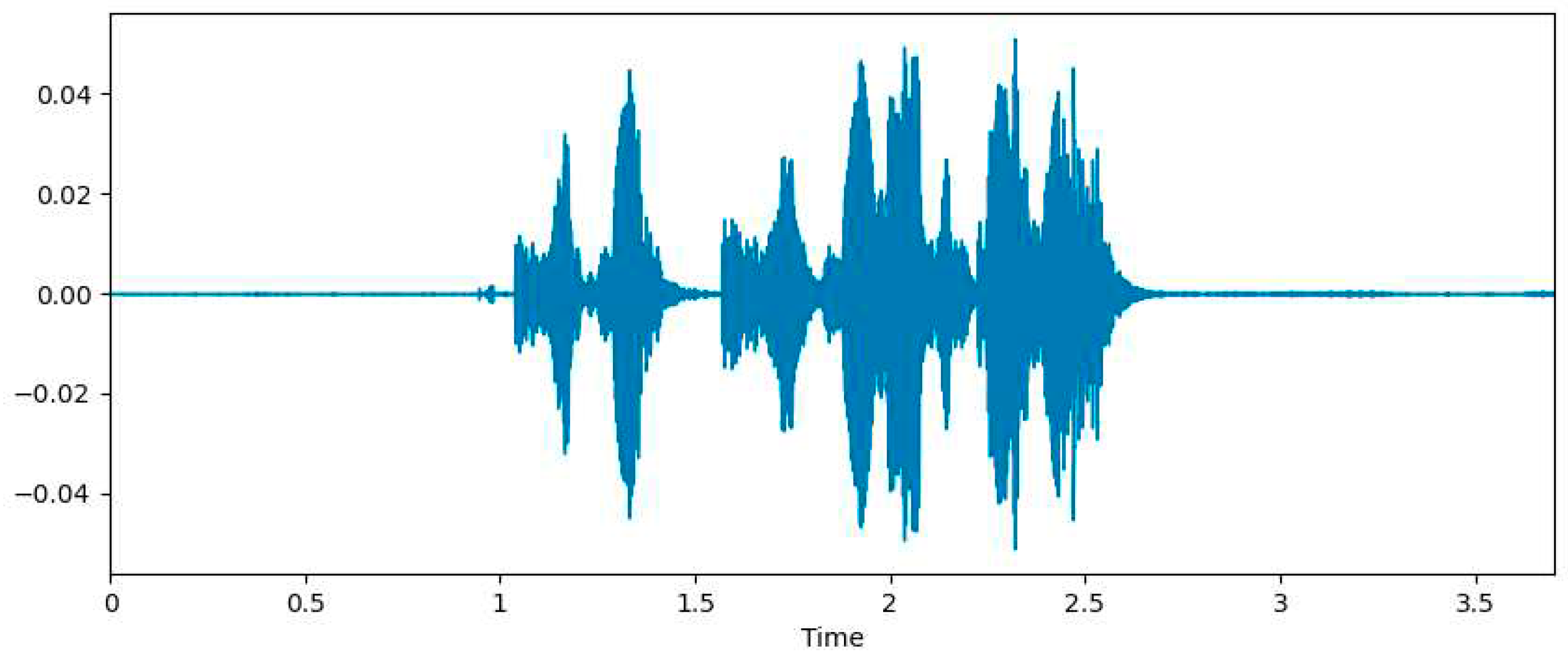
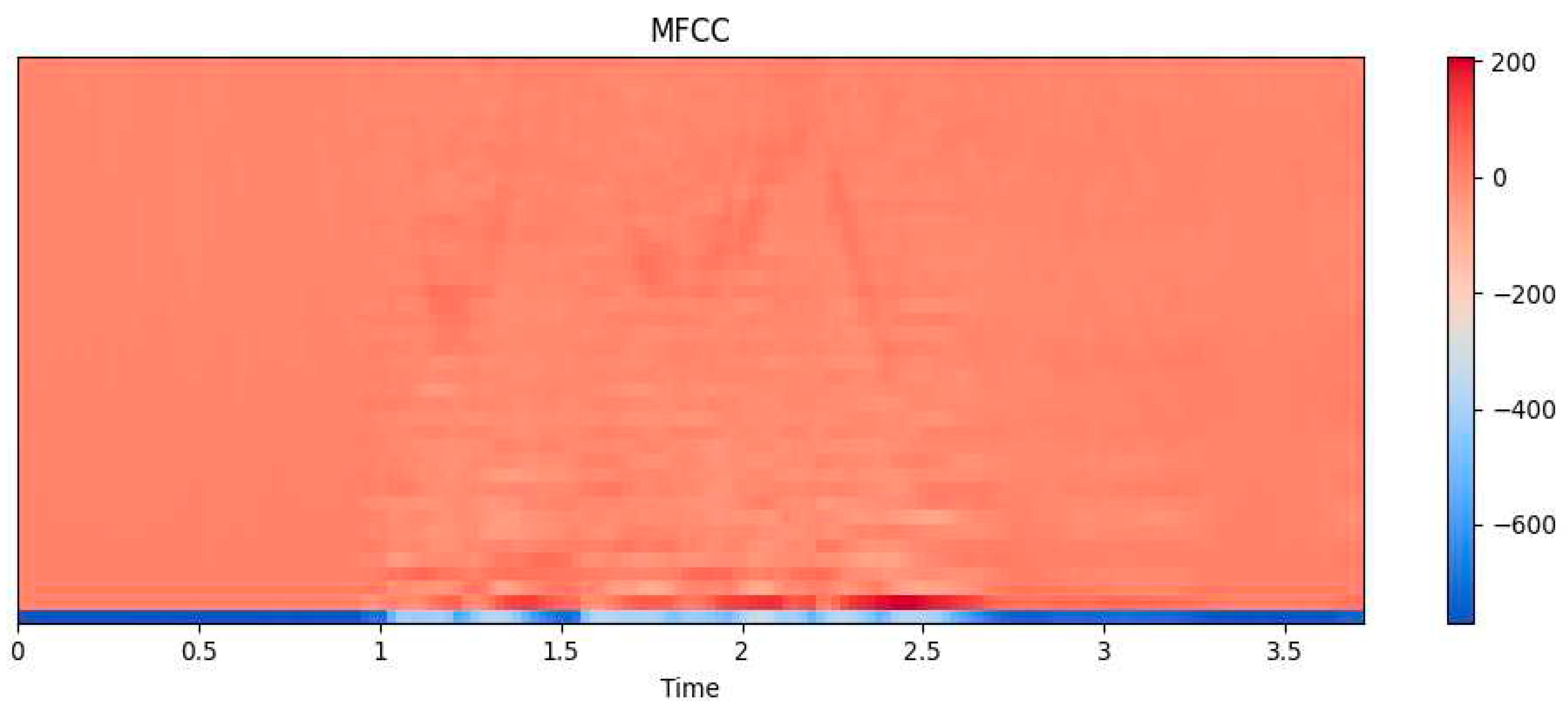
The Librosa library helped us to export the sequence of the first 40 MFCCs, shown in Figure 1 and Figure 2, to a RAVDESS database audio file.
Figure 1. Audio file from the RAVDESS dataset.
Preprints 85403 g001
Figure 2. MFCCs of the RAVDESS dataset audio file in Figure 1.
Preprints 85403 g002

3.1. Deep Belief Network (DBN)

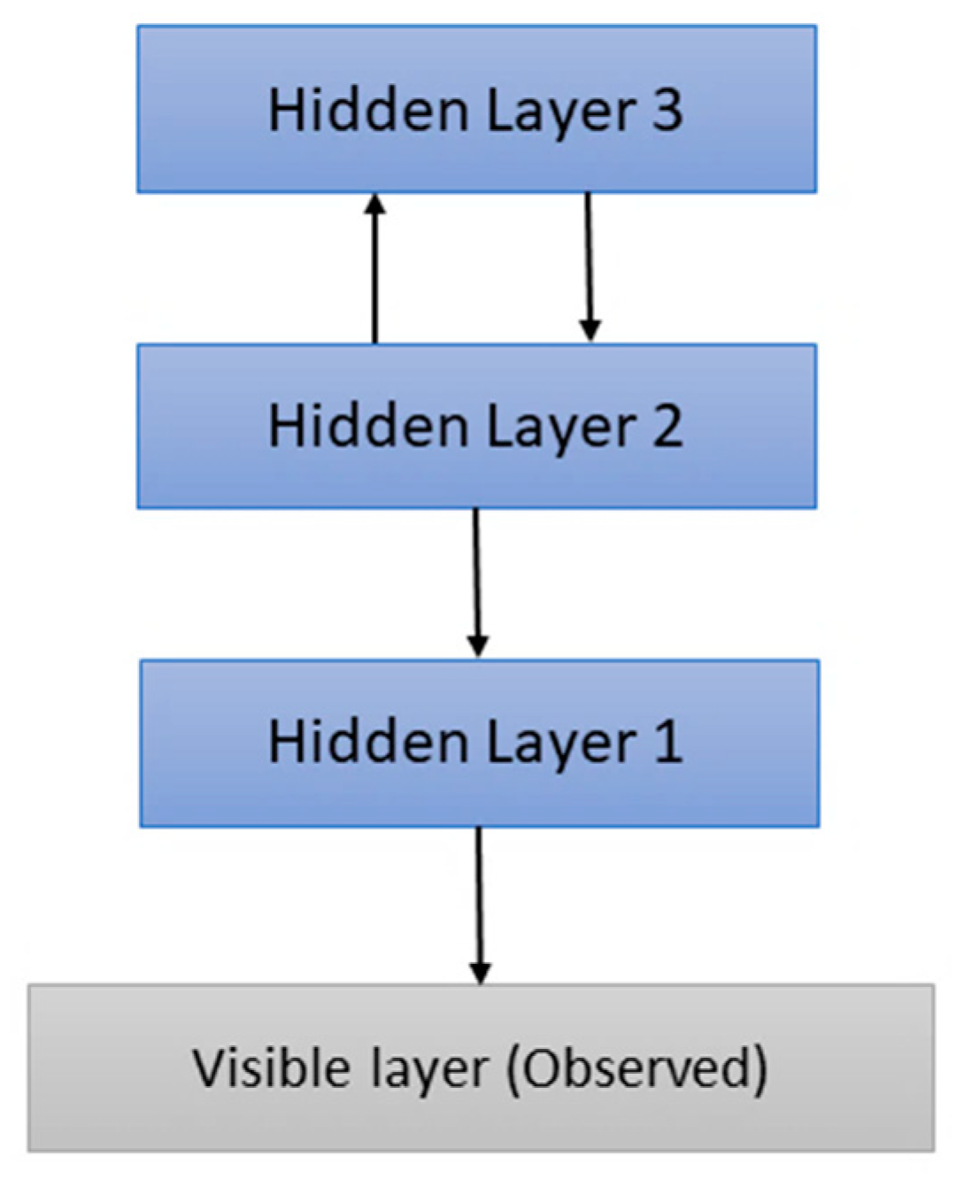
The model of our Deep Belief network (DBN) is shown in Figure 3. The code of the deep-belief-network-1.0.3 package from the Github repository (https://github.com/albertbup/deep-belief-network/) was used as the basis for the implementation of this model.
Figure 3. Deep Belief Network Model.
Preprints 85403 g003
We created a DBN with three hidden layers (Figure 3) with a size of 128 nodes each, which receives as input the time average of the 40 MFCCs. Each hidden layer can be considered a Restricted Bolzman Machine (RBM), with the hidden layer being the first layer of the next RBM. The values of the hyperparameters of the model we adopted are: 0.005 for the learning rate of the RBM hidden layers, 0.05 for the learning rate of the neural network output, 50 for the number of epochs of the RBM hidden layers. Also, we adopted the value 1000 for the number of iterations for the backpropagation algorithm, used by the neural network’s stochastic gradient descent algorithm, and 32 for the batch size. Finally, we used the Dropout normalization technique, which is a thoughtful (or random) zeroing of a percentage of connections (which in our case is 20%), between neurons (i.e., setting the output of the neuron next to 0) of two fully connected layers, as well as the ReLU activation function.

3.2. Simple Deep Neural Network (SDNN)
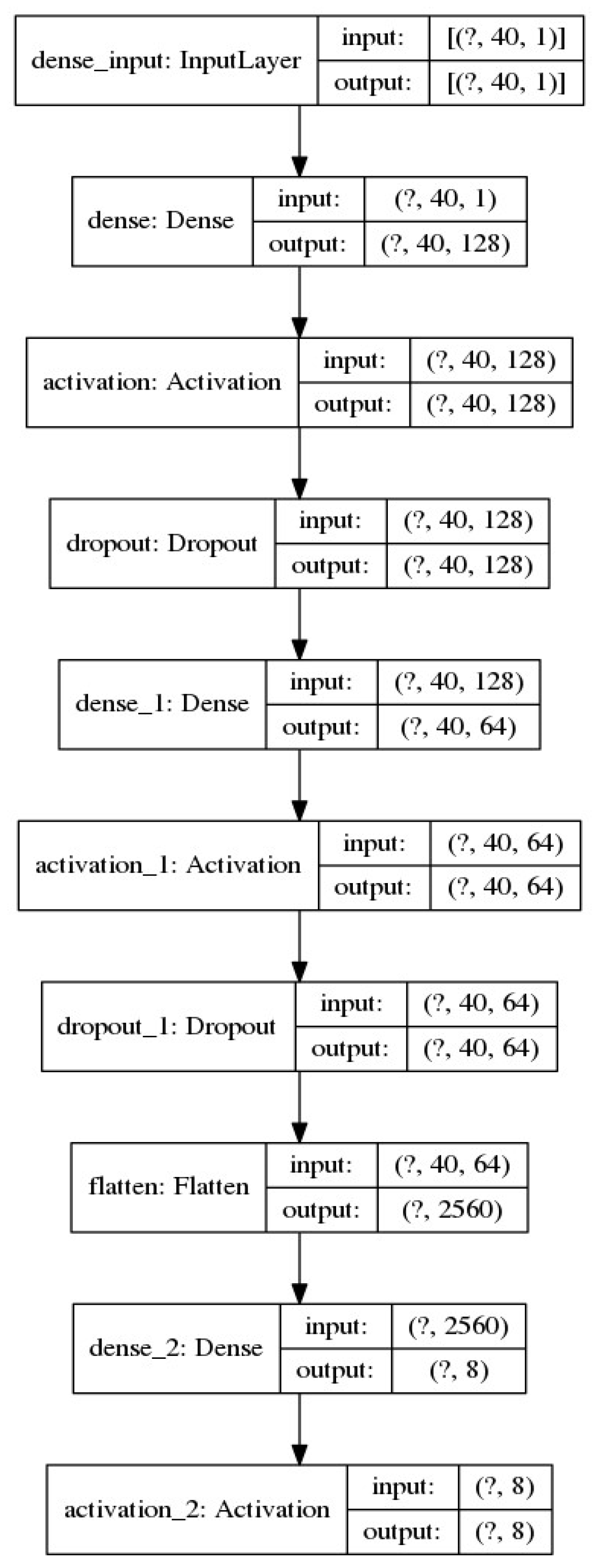
The model of our simple deep neural network is depicted in Figure 4.
Figure 1. Simple Deep Neural Network model.
Preprints 85403 g004
The diagram in Figure 4 shows a deep neural network model that receives the average time of the 40 MFCCs as input. Because we want to implement a DNN model in its simplest form, we use Dense layers, for which it is true that each input neuron is connected to the output neuron and that the parameter units simply define the dimension of the output neuron. For the first (hidden) layer of the network we use a dense layer that receives as input a tensor of dimensions (40, 1), due to the 40 MFCCs, and produces an output tensor of dimensions (40,128), due to the number of 128 parameters we defined. We use the ReLU activation function, for this layer. Also, we employ the dropout normalization technique, with 10% dropout rate. The reason for it is that in each iteration it trains a modified model that ignores the existence of some of the neurons of previous or even next layers, and this results in different groups of network parameters being trained without being affected from other parameters that have been reset, each time the code is run. Thus, our network avoids the problem of “overfitting”.
For the second (hidden) layer of the network, we use a dense layer that receives as input the output of the previous layer, a tensor (40, 128), and an output neuron of dimension (40, 64), due to the number of 64 parameters we defined for this layer. The ReLU activation function and the dropout of 10% are also used. Successively, we use the flatten function, which reshapes the tensor to have a shape equal to the number of elements contained in the tensor. In our case the number of elements included in the tensor is 2560.
The third network layer is also a dense layer that receives as input the flattened tensor (of 2560 elements), and produces a tensor of size 8 or 7, depending on the database on which we train the model. Essentially, it categorizes the 2560 elements into those 8 or 7 emotion classes. We use the “Softmax” activation function here that returns a probability distribution over the targeted classes in the multi-class classification problem.

3.3. LSTM based network (LSTM)

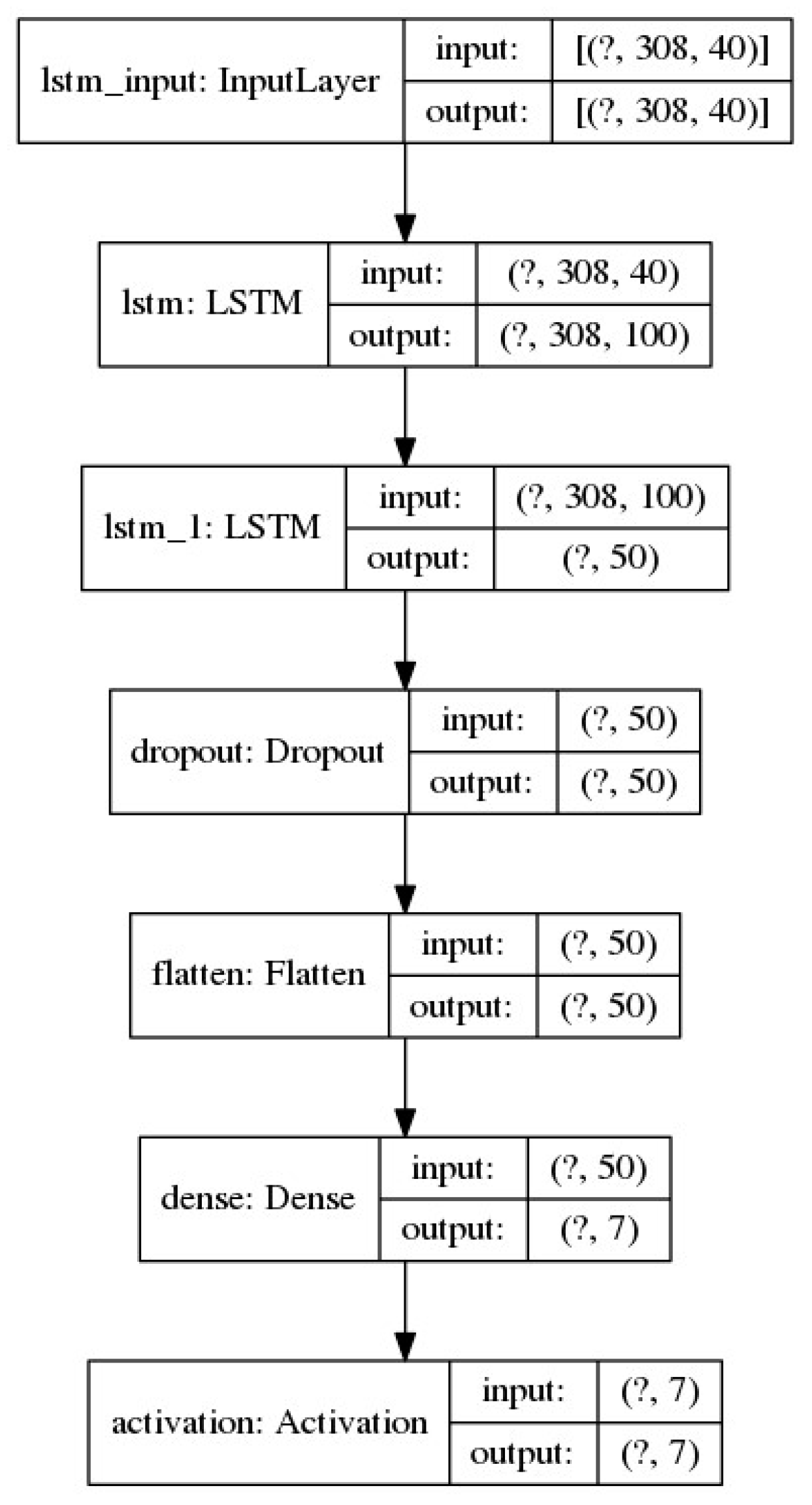
As a third model, we configure a DNN, which uses LSTM (Long Short-Term Memory layer) layers that have been found to achieve very good results in problems with sequential data. The architecture is depicted in Figure 5.
Here, instead of entering the average of the MFCCs over the file in the model, we enter the sequence of the different MFCCs over the length of the file. As the first layer of the network, we use an LSTM layer that receives as input a tensor of dimensions (228, 40) for the RAVDESS, and (308, 40) for the SAVEE database, due to the sequence size of the 40 MFCCs (228 and 308 respectively) for each database. It produces an output tensor (228, 100) and (308, 100) respectively, due to the number of parameters (100) that we defined.
As the second layer of the network, we use an LSTM layer that receives as input the output of the previous layer, and produces its output tensor of dimension 50, due to the number of 50 parameters (cells) that we defined. We use here the dropout normalization technique to reset 50% of the connections, and then the flatten function, which reshapes the tensor to have a shape equal to the number of elements contained in the tensor (50).
The third network layer is a dense layer that receives as input the flattened tensor, of 50 elements, and produces a tensor of 8 or 7 components, depending on the database we use to train the model, categorizing the 50 elements in those 8 or 7 classes of emotions. Finally, we use the “Softmax” activation function that returns a probability distribution over the targeted classes in the multi-class classification problem.
Figure 2. LSTM Based Neural Network model.
Preprints 85403 g005

3.4. LSTM based Network with Attention Mechanism (LSTM-ATN)
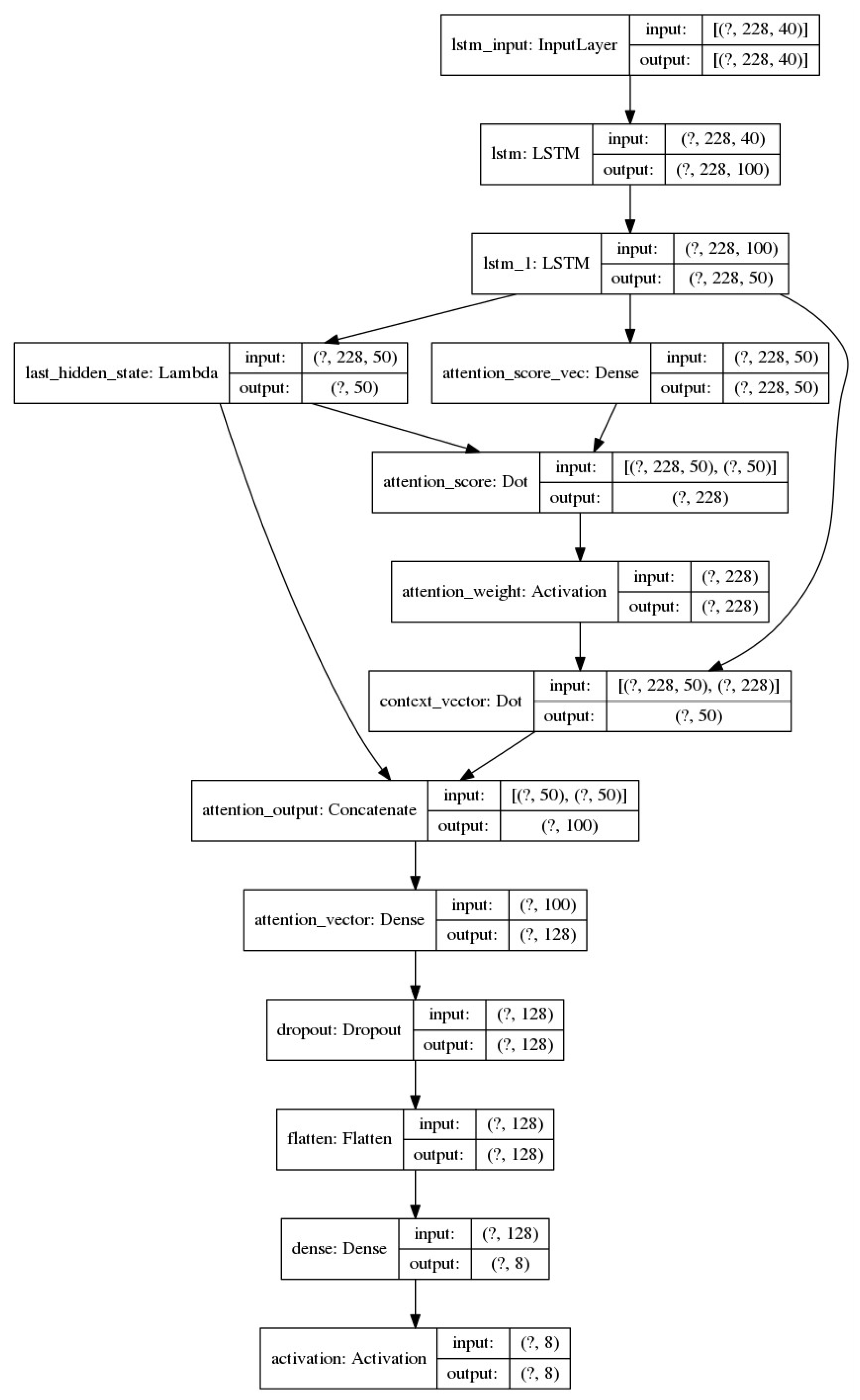
In the previous LSTM model, we add an attention mechanism, and the new created architecture is presented in Figure 6. As in the previous LSTM based model, we enter the sequence of the different MFCCs in the file duration. As the first layer of the network, we use a same LSTM layer as the one in the previous model (see Figure 5).
As the second layer of the network, we use a same LSTM layer as in the previous model, but without using dropout normalization and the flatten function.
Next, we introduce the attention layer, which applies the dot-product attention mechanism, as it is referred to in Luong [25]. The dot-product attention mechanism calculates scores through the dot product between the current/last target state h t and all previous source states h ~ s . At each time step t, in the decoding phase, this approach first takes as input the hidden state h t at the top layer of a stacking LSTM. The goal is then to draw a context vector c t that retains relevant source information to help in predicting the current target-word y t . The scoring function is calculated by s c o r e h t , h ~ s = h t T h ~ s . In this attention model, an alignment vector of variable length a t , whose size is equal to the number of time steps in the source side, is obtained by comparing the current hidden target state h t with any hidden source state h ~ s :
a t s = a l g n h t , h ~ s = exp s c o r e h t , h ~ s s e x p s c o r e h t , h ~ s
Given the alignment vector as weights, the context vector c t is calculated as the dot product of the weighted average over the previous hidden state h ~ s . Given the current target state h t and the context vector c t , we use a simple concatenation to combine information from both vectors to create an attentional hidden state as follows: h ~ t = tan h w c c t ; h t . Next, we use the dropout normalization technique to reset the order of 50% of the connections and then the flatten function, which receives the tensor with the attentional vector h ~ t , which reshapes it to have a shape equal to the number of elements contained in the tensor. In our case, the number of elements in the tensor is 128.
The third layer of the network is the same as in the previous model (see Figure 5).
Figure 3. Deep LSTM Based Neural Network with attention mechanism model.
Preprints 85403 g006

3.5. Convolutional Neural Network (CNN)
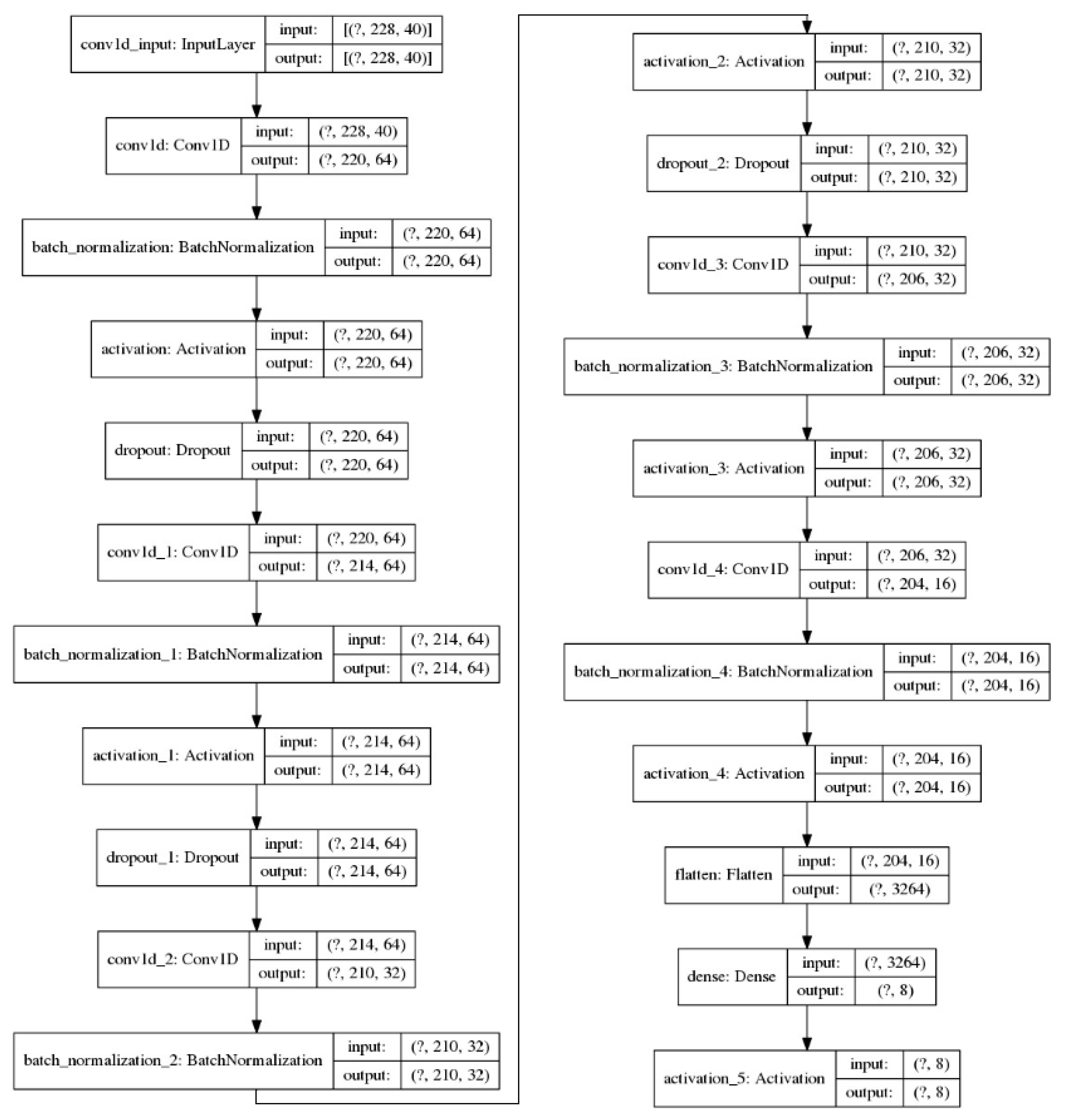
Our next model is a convolutional network that also considers the dimension of time. The architecture of the convolutional network is depicted in Figure 7.
Here, we enter the sequence of the different MFCCs in the file duration too. As the first layer of the network, we use a one-dimension convolutional layer (Conv1D), which receives as input a tensor of the dimensions (228, 40) for the RAVDESS, and (308, 40) for the SAVEE database, as previously. For the analysis of the model, we use the case of training it with the RAVDESS database, as shown in Figure 7. The first convolutional layer, in this case, will produce an output tensor of dimensions (220, 64), due to the number of 64 filters we have defined. Additionally, we set the kernel size, which refers to the size of the convolution window, to 9, as we work with a convolutional layer of one dimension. Next, we use the batch-normalization layer that speeds up training, as it allows the use of higher learning rates, given that activations are now less “sensitive” to changes in parameters. Finally, we use the ReLU activation function and the dropout normalization technique at a rate of 50%.
As the second layer of the network, we use a convolutional layer of one dimension (Conv1D), which receives as input a tensor of dimensions (220, 64) and produces an output tensor of dimensions (214, 64), due to the number of 64 filters that we defined. Additionally, we set the kernel size to 9, as explained above. Next, we use the batch-normalization layer, which speeds up training, using the ReLU activation function and a dropout of 50%.
The third layer of the network is implemented as a convolutional layer of one dimension (Conv1D), which receives as input a tensor of dimensions (214, 64) and produces an output tensor of dimensions (210, 32), due to the number of 32 filters that we defined. Additionally, we set the kernel size 7, and use the batch-normalization layer, to speed up training, using the ReLU activation function, and a dropout normalization at the rate of 50%.
The fourth layer of the network is the same as the third one.
The fifth layer of the network is implemented as a convolutional layer of one dimension (Conv1D), which receives as input a tensor of dimensions (206, 32), and produces an output tensor of dimensions (204, 16), due to the number of 16 filters that we defined. Additionally, we set the kernel size to 5, and use the batch-normalization layer, to speed up training, using the ReLU activation function.
In the sequel, we use the flatten function (in this case, the tensor contains 3264 elements). Next, a dense layer that receives as input the flattened tensor (hence it has 3264 elements), produces a tensor of size 8 or 7, depending on the database we train the model, categorizing the 3264 elements into their 8 or 7 emotion classes. Finally, we use the “Softmax” activation function.
Figure 4. Deep CNN model.
Preprints 85403 g007

3.6. Convolutional Neural Network with Attention mechanism (CNN-ATN)
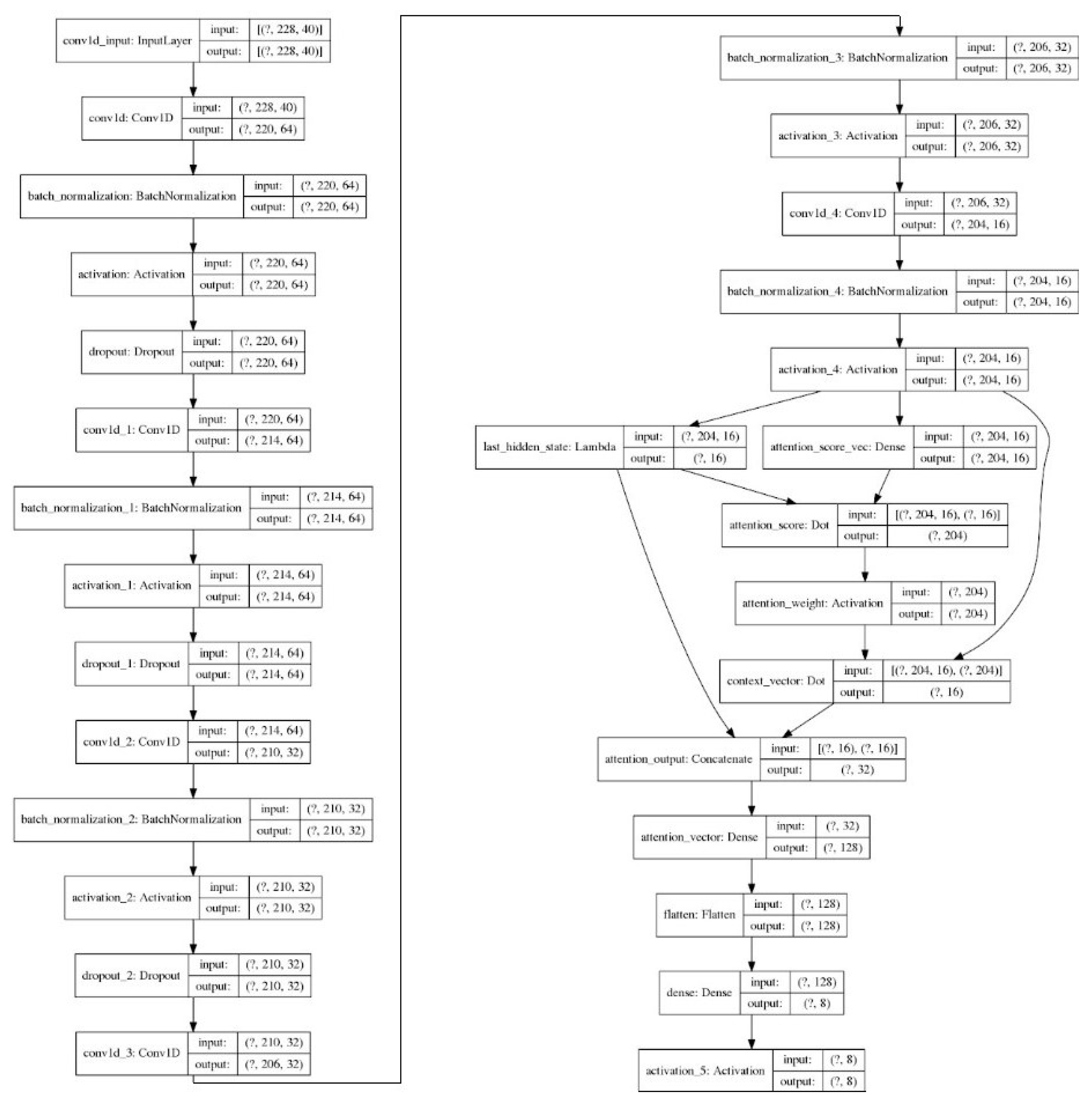
Our last model is a deep convolution network with the addition of an attention mechanism, as presented in Figure 8.
Figure 5. Deep CNN Neural Network with attention mechanism model.
Preprints 85403 g008
Here, we again enter the sequence of the different MFCCs in the file duration. Τhe first, the second, and the third layers of the network are the same as those of the plain CNN model.
The fourth layer of the network is implemented as a convolutional layer of one dimension (Conv1D), which receives as input a tensor of dimensions (210, 32) and produces an output tensor of dimensions (206, 32). The first dimension (210) is the result of reducing the input one, due to the elimination of zero values, whereas the second dimension is the number of 32 filters we have defined. Additionally, we set the kernel size to 7. Next, we use the batch-normalization layer, which speeds up training, using the ReLU activation function.
The fifth layer of the network is the same as the fifth layer of the simple CNN.
After that, we enter the attention layer, which applies the dot-product attention mechanism, in the same way as in section 3.4. An alignment vector of variable length a t is calculated by the same formula. Next, we use the flatten function, which receives the tensor with the attentional vector h ~ t , which reshapes it to have a shape equal to the number of elements contained in the tensor (128 in our case).
Then, a dense layer is used, which receives as input the flattened tensor that has 128 elements and produces an 8 or 7 components tensor, as in previous models, where the “Softmax” activation is used.

3.7. Implementation Tools

For all the above implementations, except the DBN model, for which we utilized the CPU, we utilized Tensorflow and Keras. TensorFlow uses dataflow graphs to represent the calculation, the shared state, and the functions that transform that state. It maps the nodes of a data flow graph to multiple machines in a cluster, and within a machine on multiple computing devices, including multiple CPU cores, general purpose GPUs, and specially designed ASICs (Application-Specific Integrated Circuits), known as Tensor Processing Units (TPUs). Keras is an open-source library that provides a Python interface for artificial neural networks. Built on top of TensorFlow, Keras is an industry-strength framework that can scale to large clusters of GPUs or an entire TPU pod. As a Python distribution platform, we used Anaconda. For training purposes, we used the Adam optimizer, and “sparse categorical crossentropy” as our loss function. The BDN model utilized a learning rate of 0.05, the simple DNN model utilized a learning rate of 1e-4 (0.0001), where the rest of the models (LSTM with and without attention, CNN with and without attention) utilized a learning rate of 1e-3, which becomes 1e-4 in 100 epochs. Also, the batch size we used for neural network training for all the models, except DBN, is 32. The specifications of our running system are the following: GPU: NVIDIA GTX 1070, CPU: Intel(R) Core (TM) i7-9750H, RAM: 16 GB.

4. Experimental Study and Results

In this section, we first present the datasets that we have used as well as the results of the six implemented models, presented in Section 3, and then compare the best of them (called ‘our method’) with state-of-the-art models. The models were trained, splitting both databases into a training set and a validation (test) set at a rate of 80% - 20%, respectively.

4.1. Datasets

For our experiments, we used two datasets, the SAVEE (Surrey Audio-Visual Expressed Emotion) database1 [26], and the RAVDESS (Ryerson Audio-Visual Database of Emotional Speech and Song) database2 [27].
SAVEE is an audio-visual dataset that comprises 480 English utterances from four male actors, aged from 27 to 31 years, in seven different emotions, which are anger, disgust, fear, happiness, sadness, surprise, and neutral. Utterances are categorically labeled. Recordings consisted of 15 TIMIT database3 sentences per emotion (with additional 30 sentences for neutral state). Emotion assessment of recordings was performed by subjective evaluation under audio, visual and audio-visual scenarios. Speech data was labeled at phone-level in a semi-automated way. The audio data sampling rate used is 44.1 kHz.
RAVDESS contains a total of 1440 speech utterances and 1012 song utterances. Each audio file was rated on a scale of 10 on intensity, emotional validity, and genuineness. The emotion in the speech includes surprise, happy, calm, fearful, sad, disgust and angry. The song section contains happy, calm, sad, angry, and fearful emotions. Every file has two levels of emotional intensity: normal and strong. The RAVDESS dataset is very rich in nature given that it does not suffer from gender bias, consists of wide range of emotions and at different level of emotional intensity.

4.2. Experimental Results-Accuracy and Loss Curves
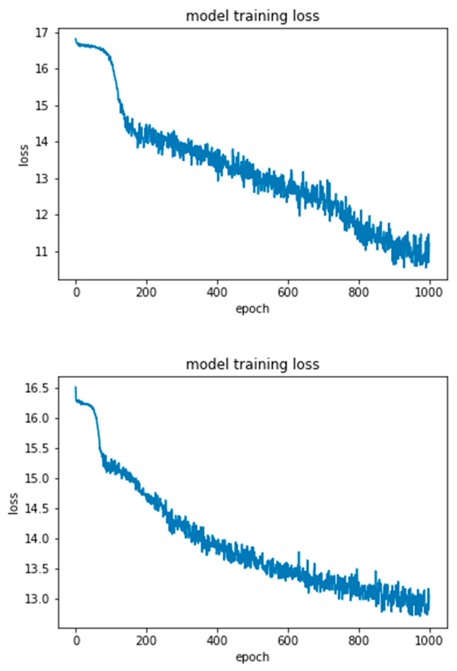
In the sequel, we present the results in the form of graphs for the accuracy and loss of our six models, through Figures 9 to 24. Where there is need, we add some comments. It is important to note here that compared to the other models, the Deep Belief Network (DBN) algorithm package provides only loss information, so we have only one graph for each dataset.
Figure 6. DBN loss training charts for RAVDESS (left) and SAVEE (right) databases.
Preprints 85403 g009
Figure 7. DNN training charts for RAVDESS database.
Preprints 85403 g010
Figure 8. DNN training charts for SAVEE database.
Preprints 85403 g011
Figure 9. LSTM network training charts for RAVDESS database.
Preprints 85403 g012
Figure 10. LSTM network training charts for SAVEE database.
Preprints 85403 g013
Figure 11. LSTM network with attention mechanism training charts for RAVDESS database.
Preprints 85403 g014
Figure 12. LSTM network with attention mechanism training charts for SAVEE database.
Preprints 85403 g015
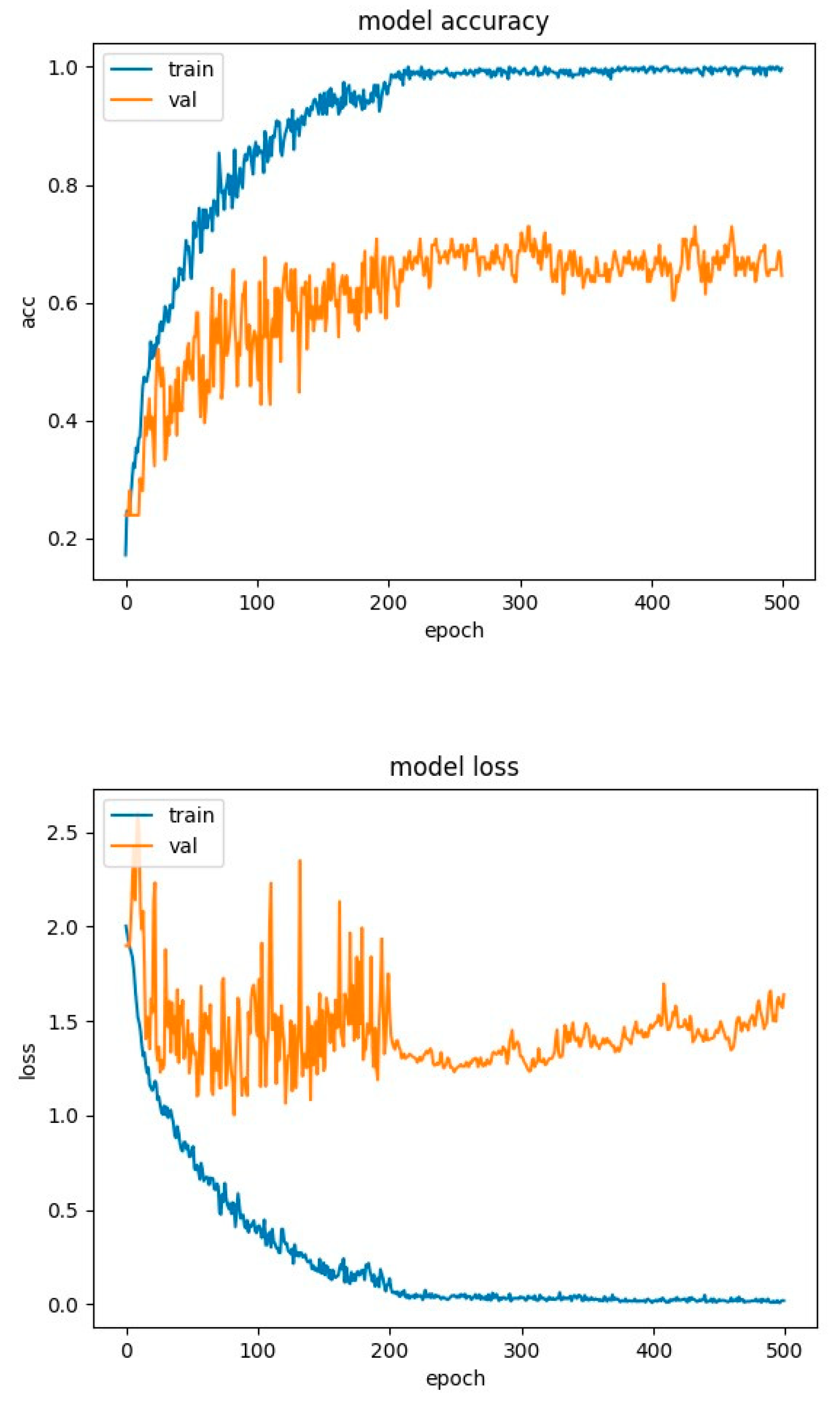
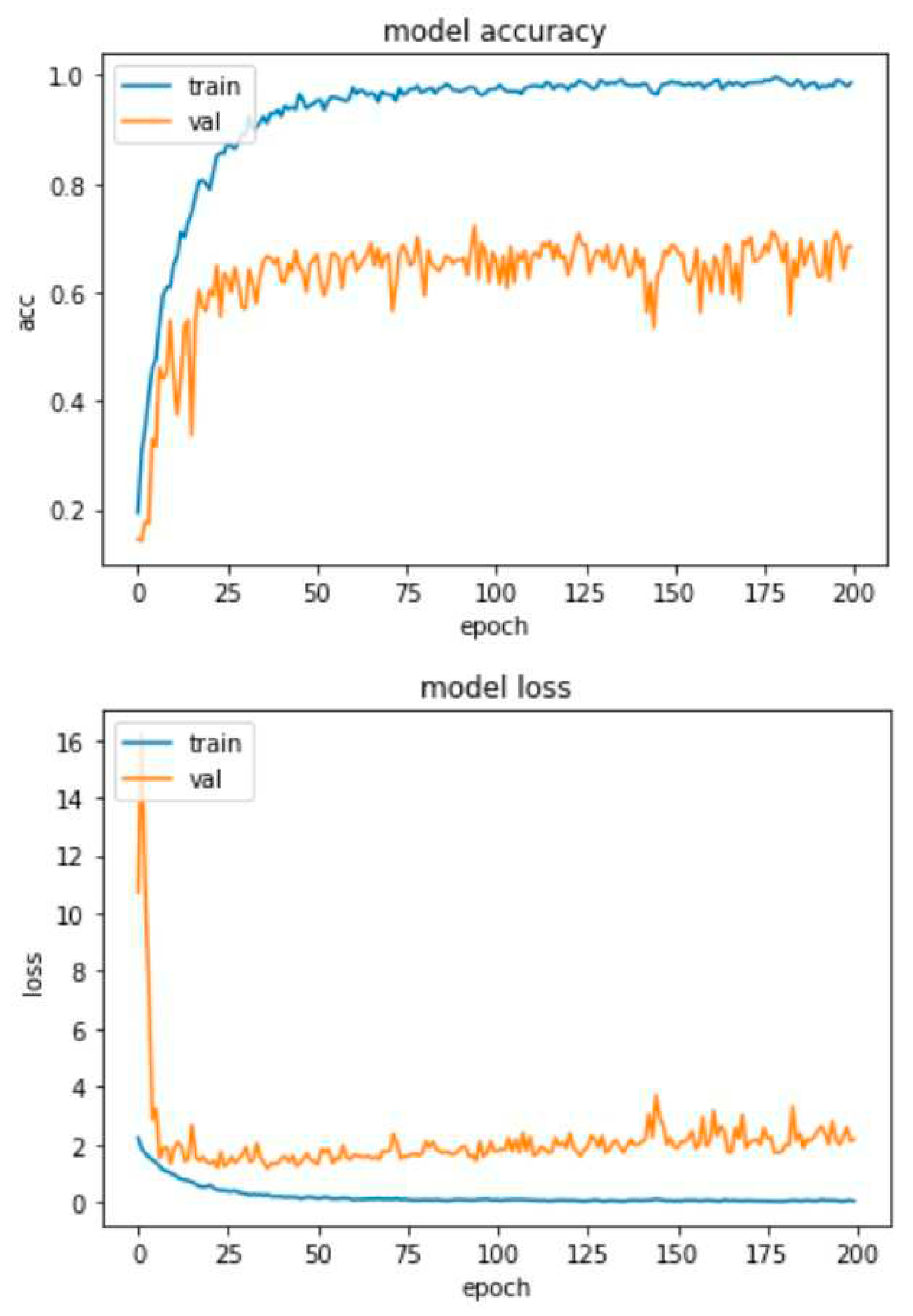
Figure 13. CNN network training charts for RAVDESS database.
Preprints 85403 g016
Figure 14. CNN network training charts for SAVEE database.
Preprints 85403 g017
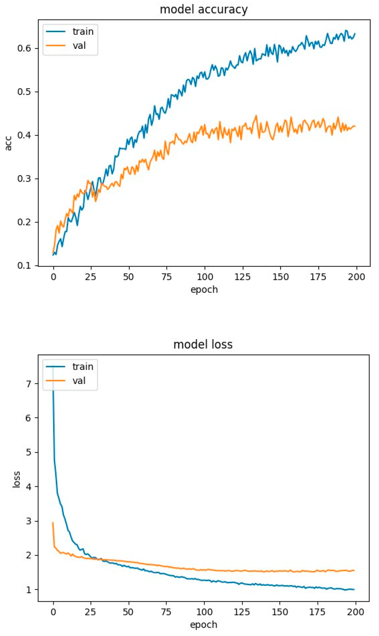
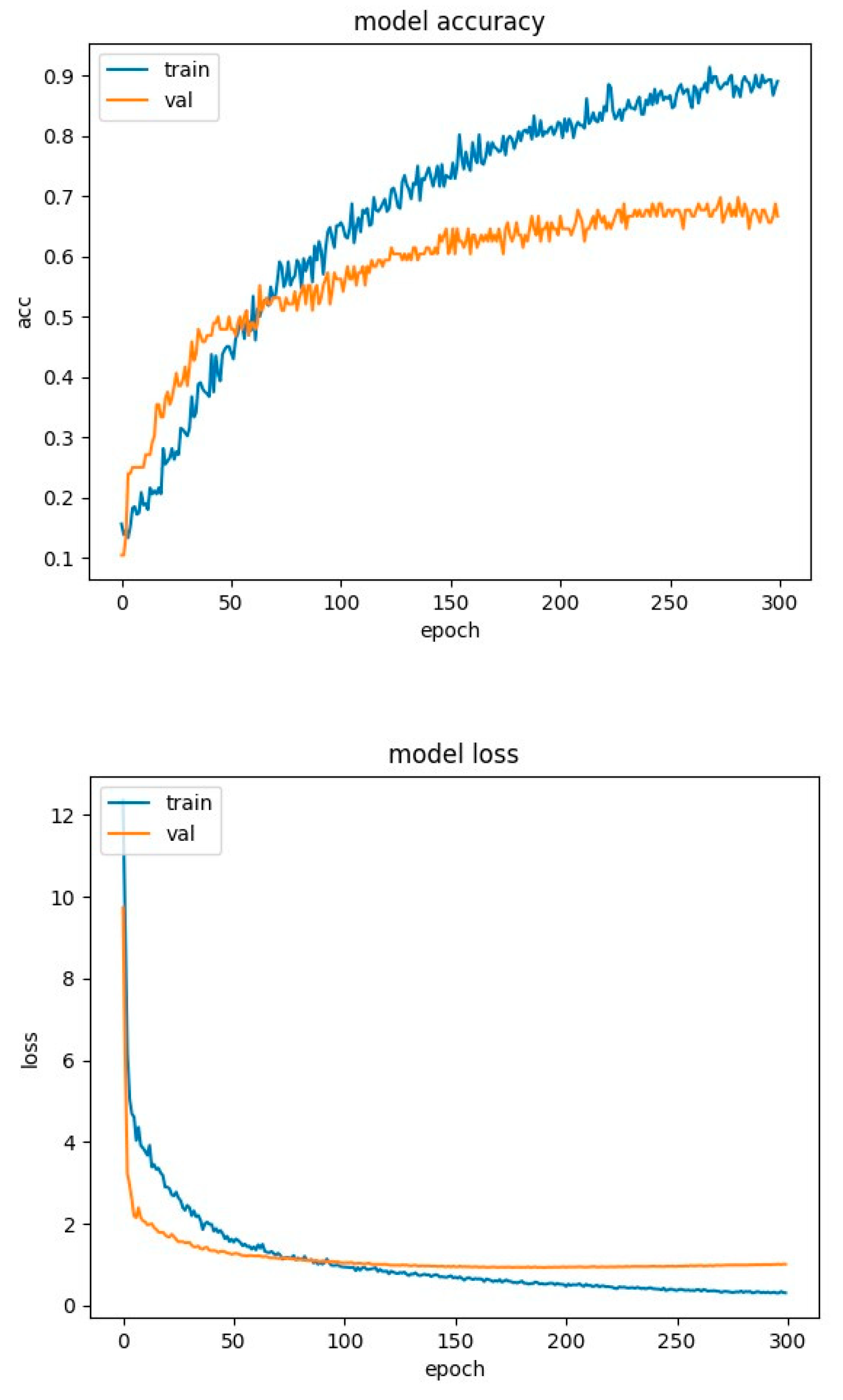
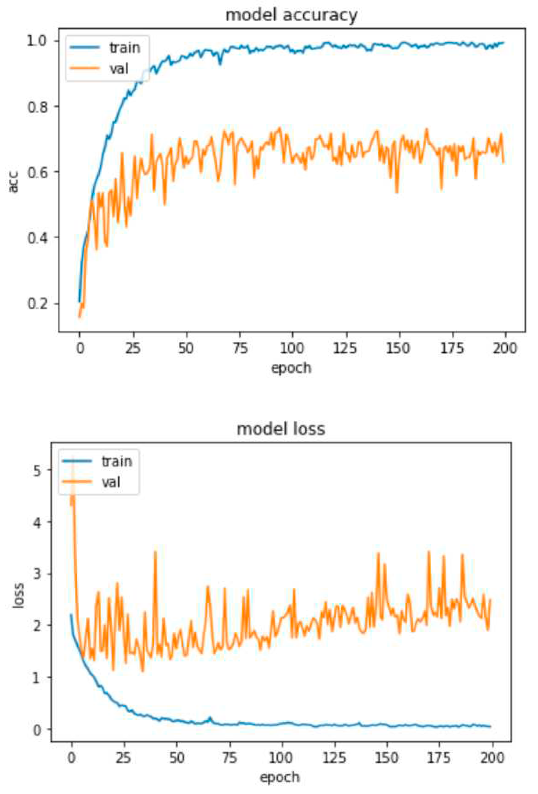
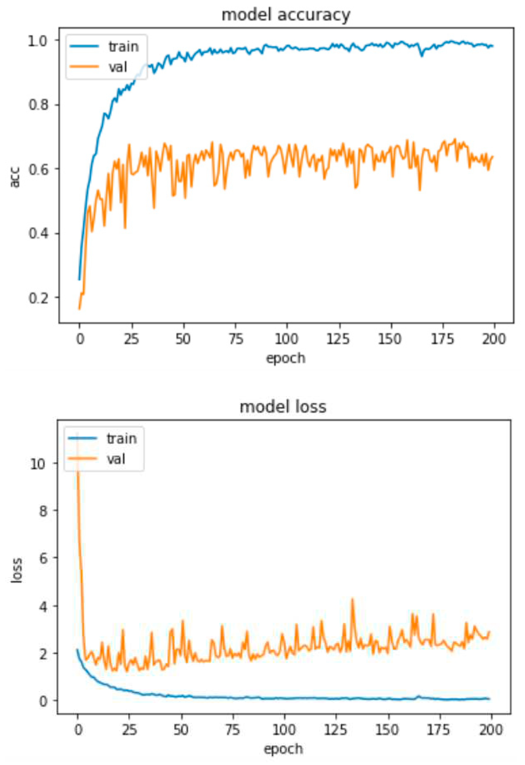
The model of Figure 13 and Figure 14 uses the batch-normalization and dropout techniques with a reset of 50%, to prevent large overfitting of the model, but still no good generalization is achieved. For this reason, two more variations of our model were tested.
Initially, zero padding was tested on the input vectors at the hidden levels. This was to keep the dimensions of the vector containing the input sequence the same as the model proceeds to the next hidden levels (for RAVDESS 228, and for SAVEE 308). This test was performed on the RAVDESS database, and the accuracy and loss curves are presented in Figure 18.
As we can see from the graphics of the test with zero padding compared to our model in Figure 16, it is obvious that the accuracy remains the same (70.5%), as well as the overfit (30%). However, comparing the graph of the loss between the two implementations, we observe that the error from epoch 50 onwards, in the zero-padding test, gradually increases and does not stabilize after epoch 100 on 2, as is done with the model in Figure 16. On the contrary, it continues to grow and exceeds 2.
Then, after the first test for the RAVDESS database had not yielded the desired results, a second test was performed using zero padding in combination with the replacement of the ReLU activation function by the LeakyReLU. The ReLU activation function sets, all negative values to zero. This makes our network adaptable to ensure that the most important neurons have positive values (> 0). However, this can also be a problem, as the gradient of 0 is 0 and therefore neurons that reach large negative values cannot recover and stick to 0. This causes the neurons to die and for this reason this phenomenon is called “The dying ReLU problem”.
Figure 15. CNN network training charts for RAVDESS database with zero padding.
Preprints 85403 g018
To avoid this phenomenon, LeakyReLU was proposed, according to which negative values instead of zero are multiplied by a factor of 0.01:
f x = 0.01 ,   i f   x < 0   x ,     x 0
Comparing it with ReLU, we can see that LeakyReLU has a slight negative slope, avoiding the entrapment of neurons with negative values at 0. There have generally been reports of success adopting this activation function, but the results are not always consistent. The reason we want to apply it to the CNN model is that through its operation we reduce the phenomenon of overfitting a little more, and stabilize more the instabilities of our system, which appear as abrupt changes (spikes) in the graphics.
This test was performed on RAVDESS and SAVEE databases and the accuracy and loss curves are depicted in Figure 19 and Figure 20 respectively.
Figure 16. CNN network training charts for RAVDESS database with zero padding and LeakyReLU.
Preprints 85403 g019
Figure 17. CNN network training charts for SAVEE database with zero padding and LeakyReLU.
Preprints 85403 g020
As we can see from the graphs of the test with zero padding and LeakyReLU in the RAVDESS base, compared to our model in Figure 16, it is obvious that the accuracy decreases slightly (67%) and the overfitting increases slightly (33%). Comparing the graphs of loss between the two implementations, we notice that the instability (spikes) of the system has been improved. However, the error from epoch 50 onwards, in the test with zero padding and LeakyReLU, increases gradually and does not stabilize after epoch 100 on 2, as it is done with the model in Figure 16. On the contrary, it continues to increase, approaching values such as 3 and 4.
Comparing now the graph of test accuracy with zero padding and LeakyReLU on the SAVEE base with that of Figure 17, we notice that the accuracy increases dimly (55.7%) compared to the model in Figure 17 (55.2%), so there is a very minimal reduction in overfitting, of 0.5%. Then comparing the loss graphs between the two implementations, we notice that the instability (spikes) of the system has been slightly improved. The error from epoch 50 onwards, in the test with zero padding and LeakyReLU, increases gradually and does not stabilize, approaching 3.5. This is a small improvement of the system as the loss in Figure 17 approaches 4.5 in epoch 200, but from epoch 200 onwards stabilizes.
The above comparison of the two tests with the implementation of Figure 16 in the RAVDESS database concludes that our model with the use of ReLU and without zero padding gives overall better results in terms of accuracy and loss. Regarding the comparison of the test with zero padding and LeakyReLU with the implementation of Figure 17 for the SAVEE base, we observe that the test with zero padding and LeakyReLU achieves faintly improved overall results, in terms of both accuracy and loss. This may be due to the fact that this database has a smaller number of samples than RAVDESS. Therefore, we conclude that the model implemented with ReLU and without zero padding performs in general better and that the techniques tested do not give the desired results, i.e. reduce the overfitting effect and the loss to a significant degree.
Figure 18. CNN network with attention training charts for RAVDESS database.
Preprints 85403 g021
Figure 19. CNN network with attention training charts for SAVEE database.
Preprints 85403 g022
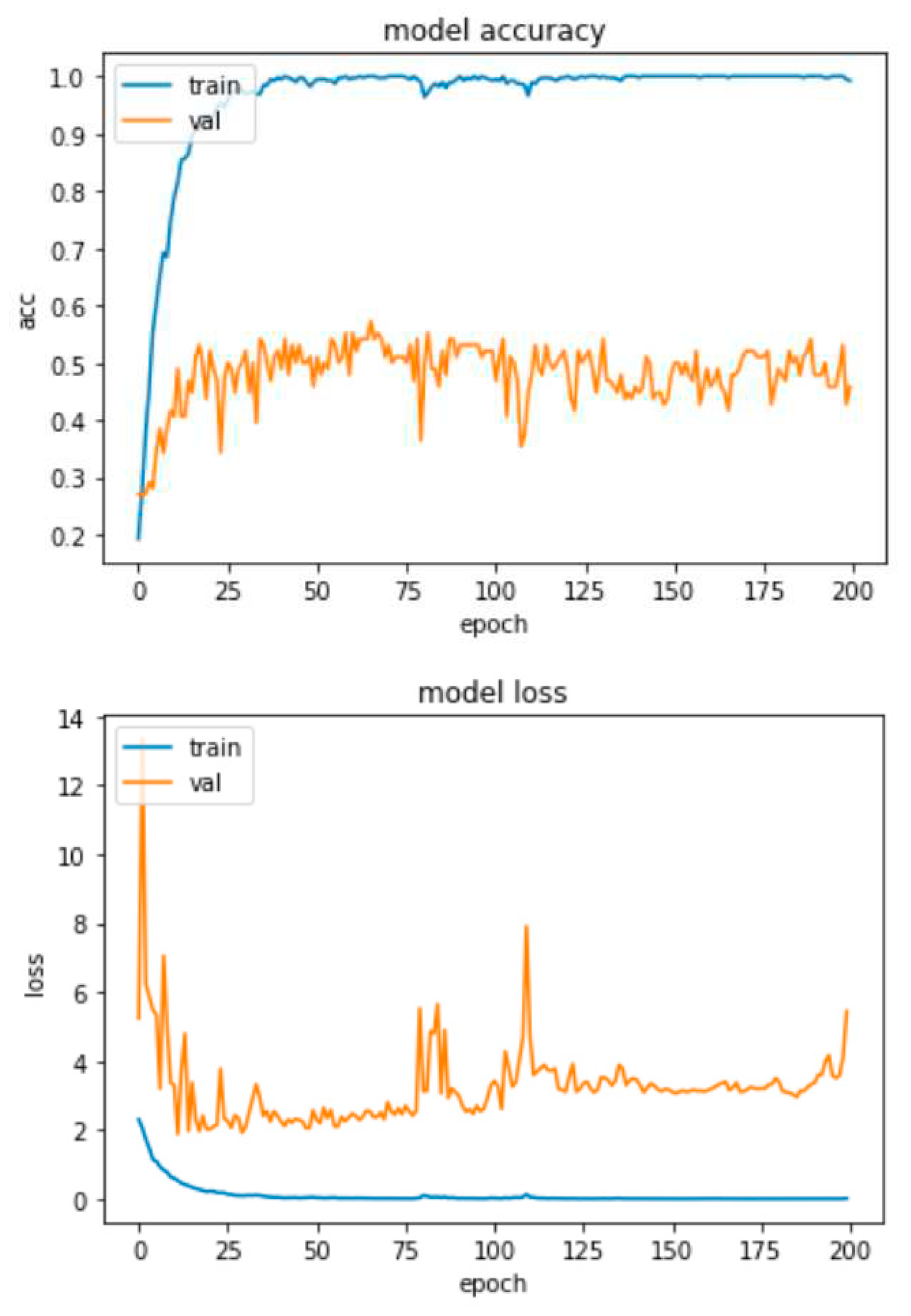
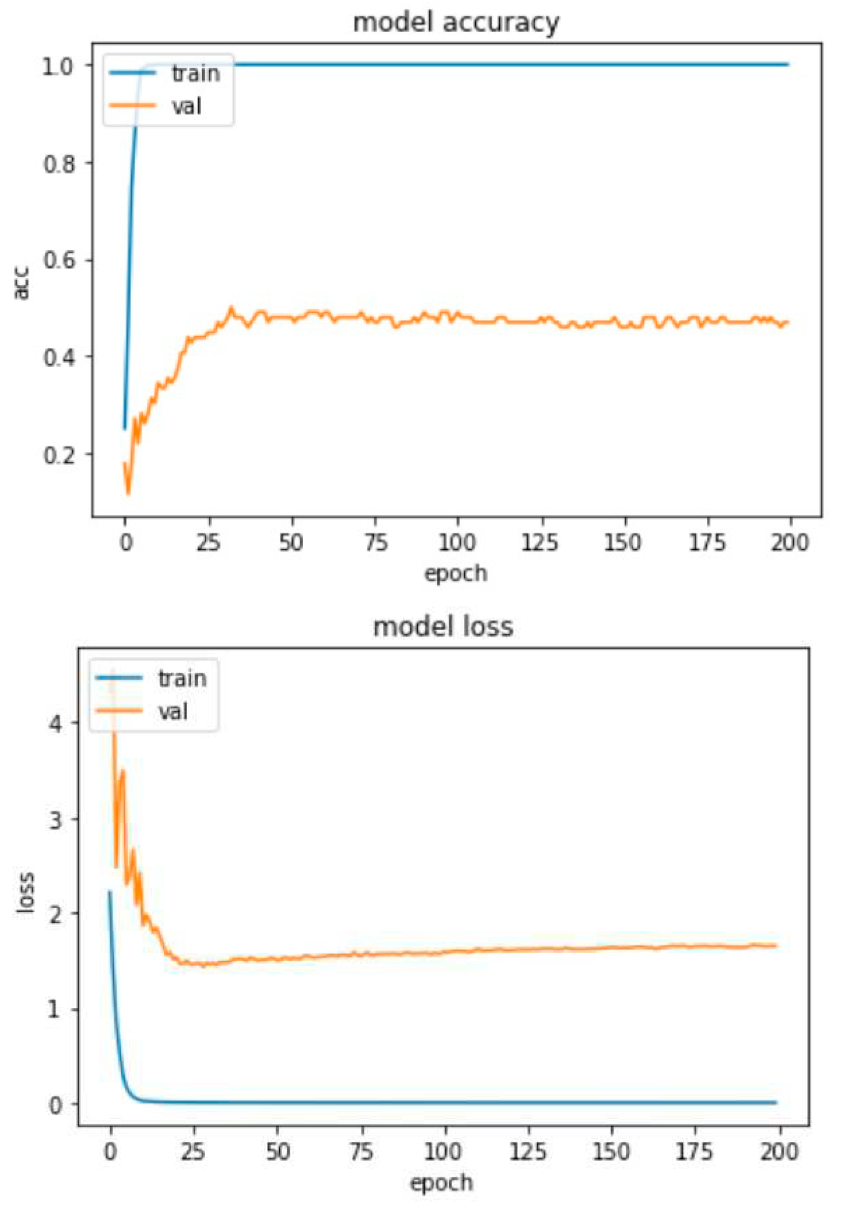
Because we see that the models show a degree of overfitting that cannot be further reduced, we performed a test, where we removed the dropout normalization technique from the model, so that only the batch-normalization technique remained, to see the effects. The results of this model (without the dropout) for the RAVDESS and SAVEE databases are depicted in Figure 23 and Figure 24, respectively.
Figure 20. CNN network with attention training charts for RAVDESS database without Dropout.
Preprints 85403 g023
Figure 21. CNN network with attention training charts for SAVEE database without Dropout.
Preprints 85403 g024
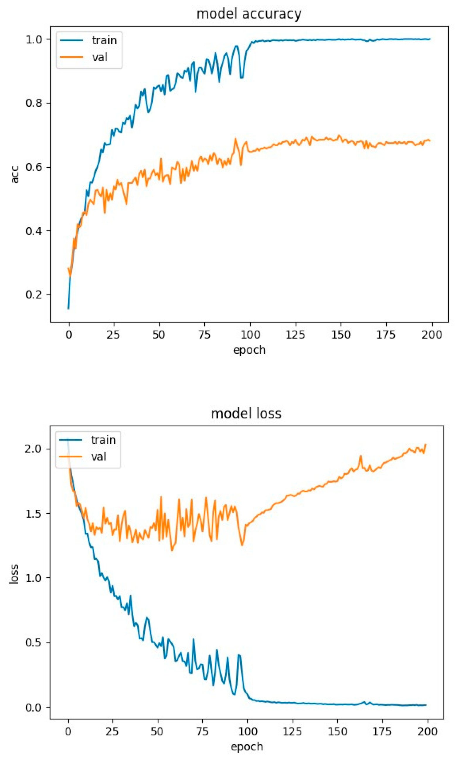
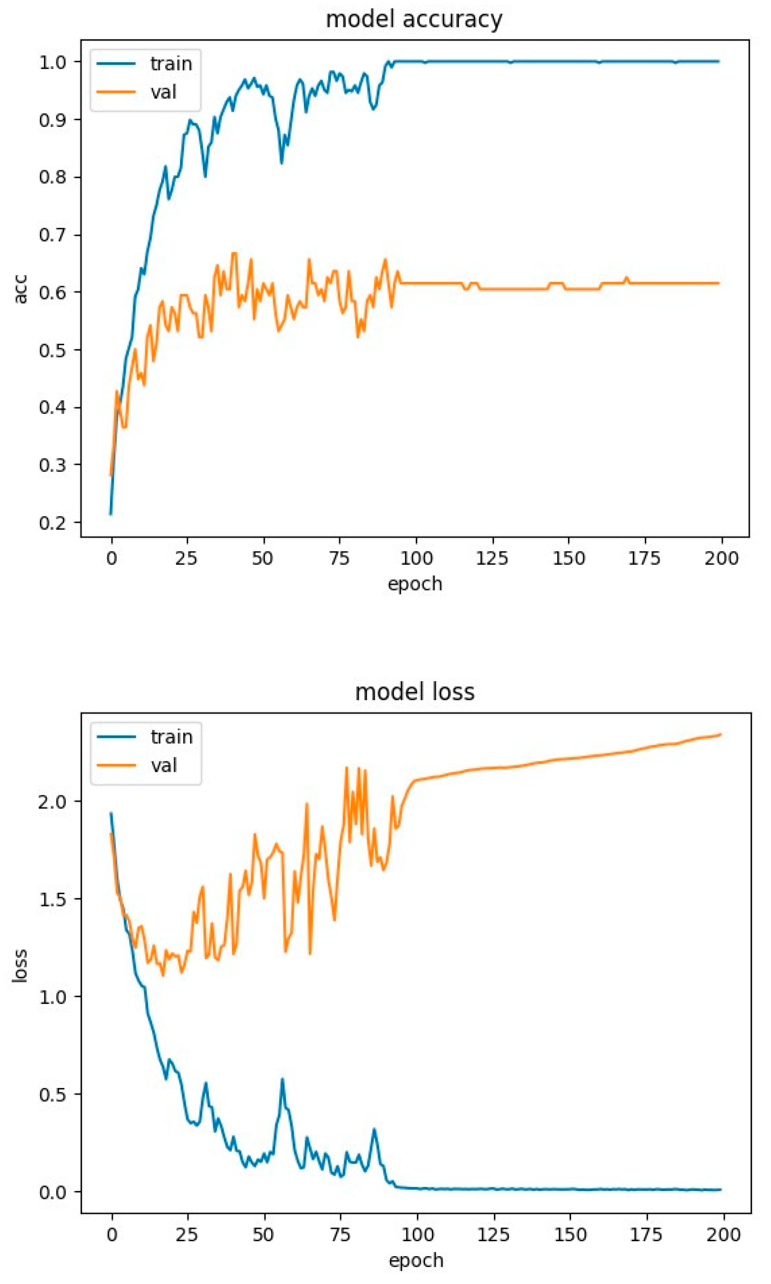
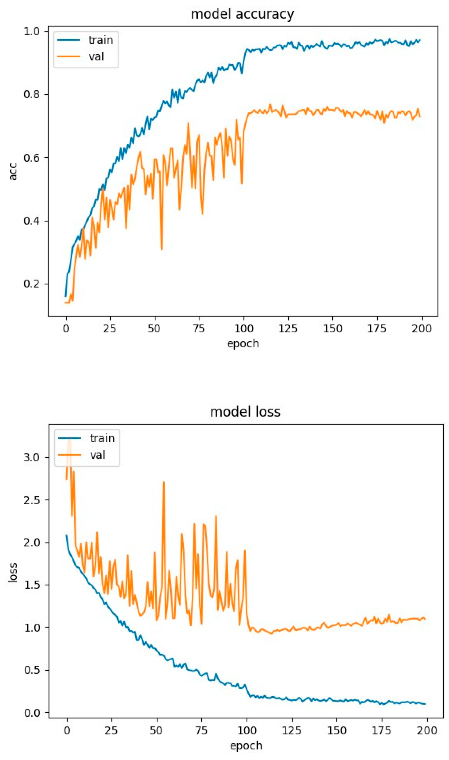
It is obvious that with the removal of the dropout function, the model shows a significant increase in the overfitting effect, given that for both the RAVDESS and SAVEE datasets we observe a significant reduction in the accuracy of the model and some increase in loss. More specifically, for the RAVDESS dataset, the model without the dropout function achieves 65% accuracy, in contrast to the model of Figure 21, which achieves 77% accuracy. This means that the model without the dropout technique overfits to a percentage of 45% on this dataset. Also, the loss of the model without the dropout technique fluctuates (spikes) around 2.5, while the model of Figure 21 fluctuates (spikes) around 1.5, and from epoch 100 onwards revolves around 1, with a minimal upward trend to 1.2.
For the SAVEE dataset, the model without the dropout technique achieves an accuracy of 47%, in contrast to the model of Figure 22, which achieves an accuracy of 74%. This means that the model without the dropout technique overfits to a percentage of 63% on this dataset. Also, the loss of the model without the dropout technique from epoch 25 onwards has a steady upward trend from 1.3 to 1.6, while the model in Figure 22 fluctuates (spikes) around 1.5. From the above it is obvious that proposed CNN-Attention model applying the dropout technique against overfitting is the best possible option.

4.4. Experimental Results-Confusion Matrices
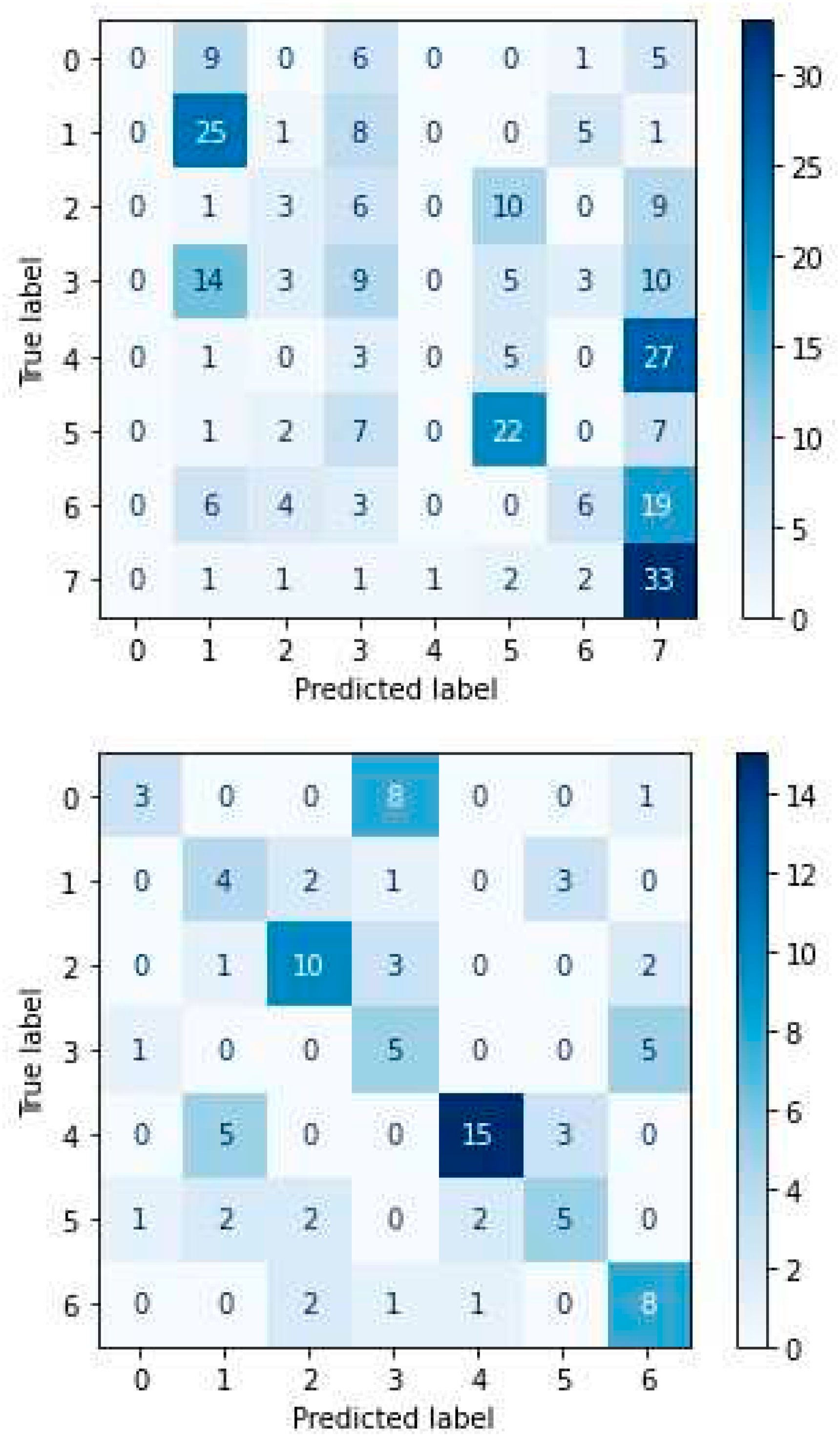
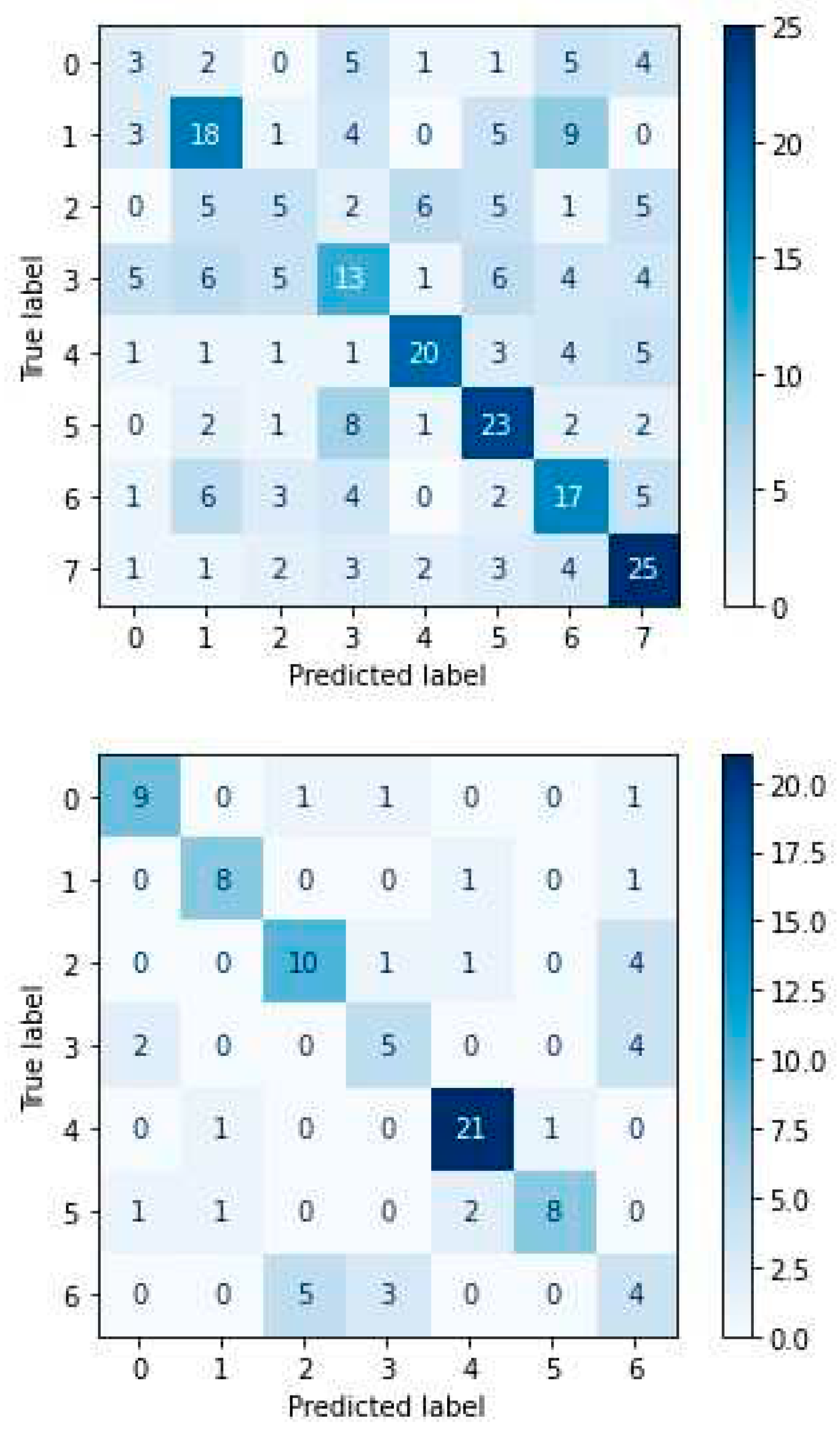
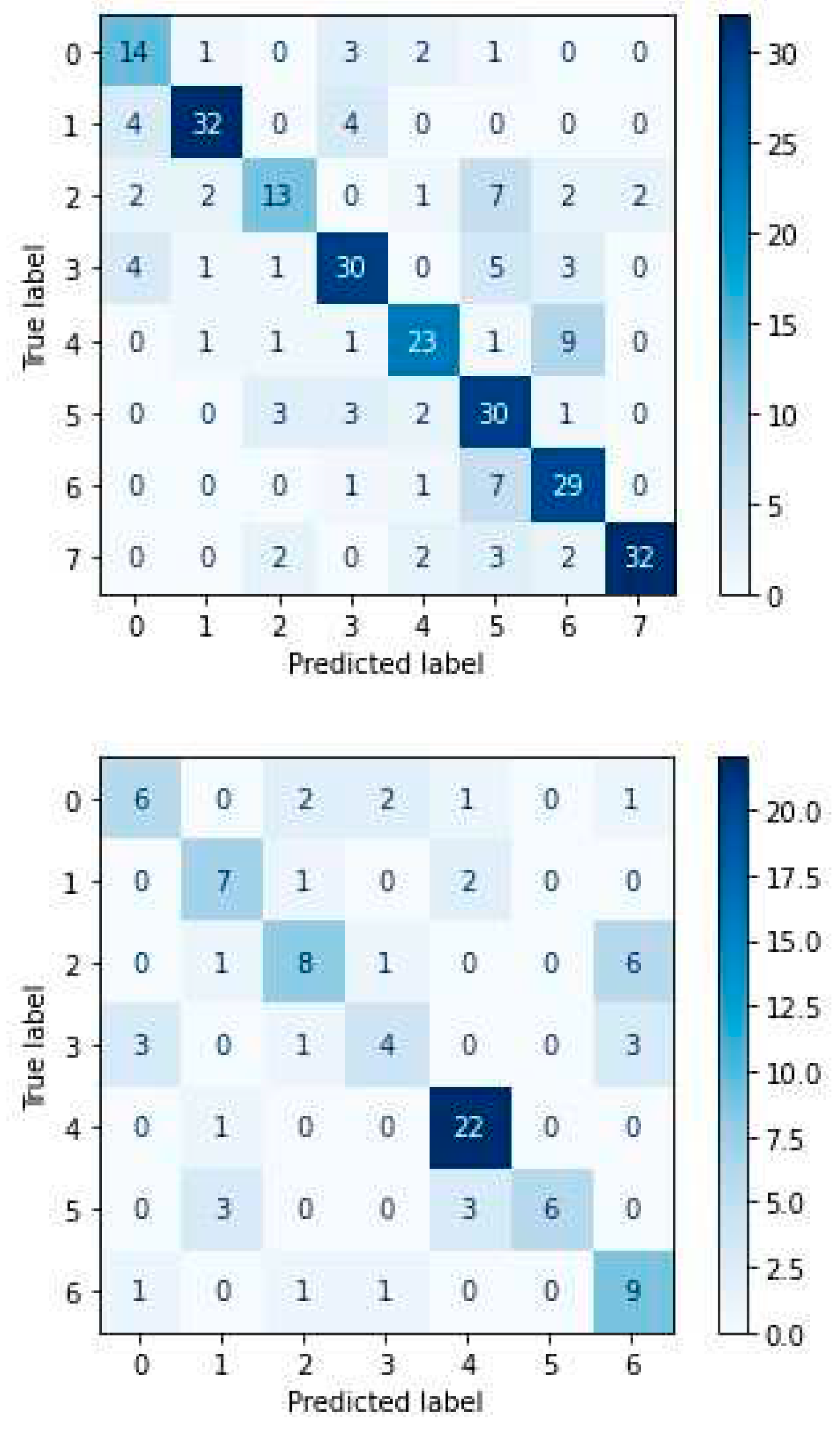
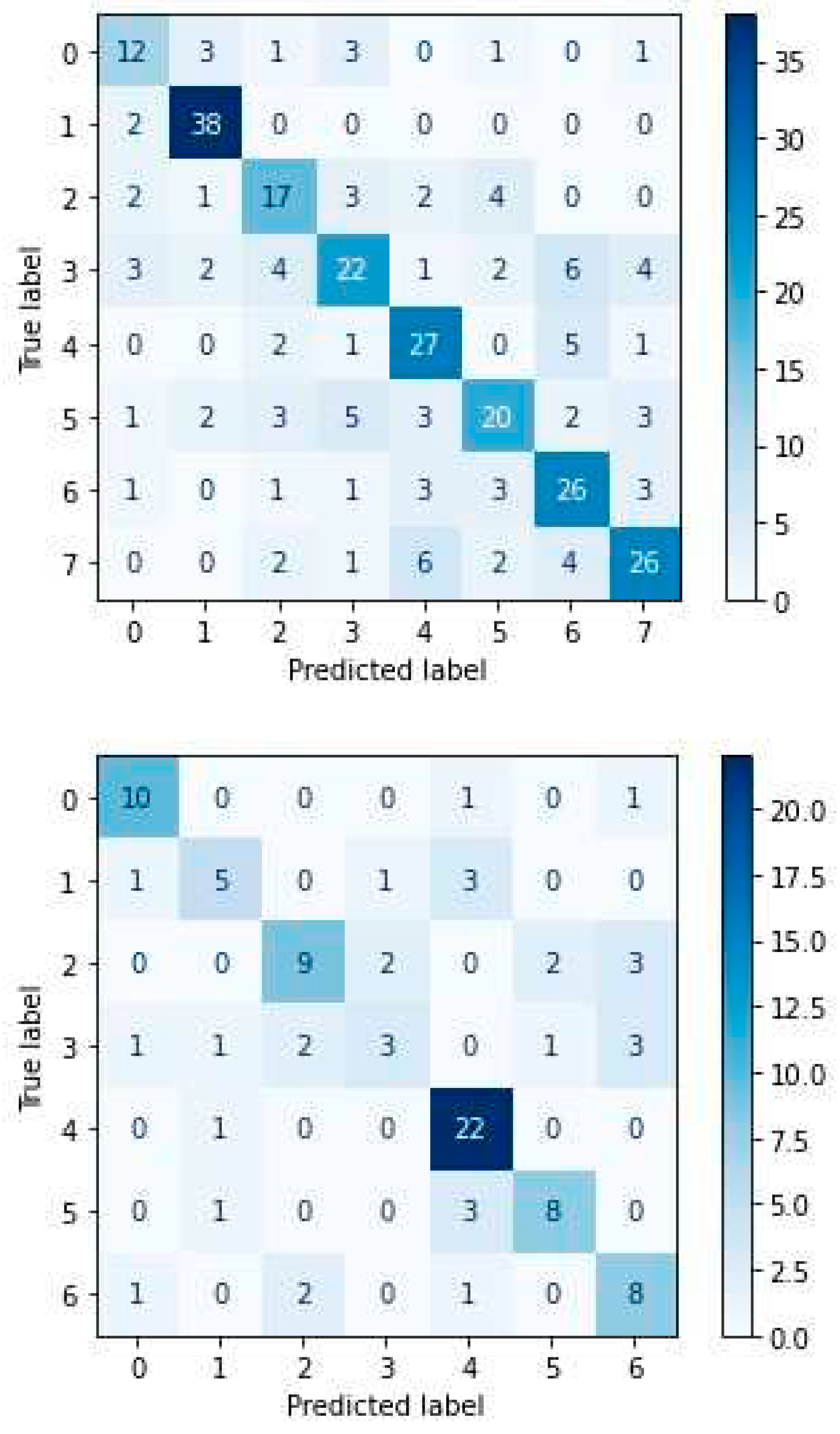
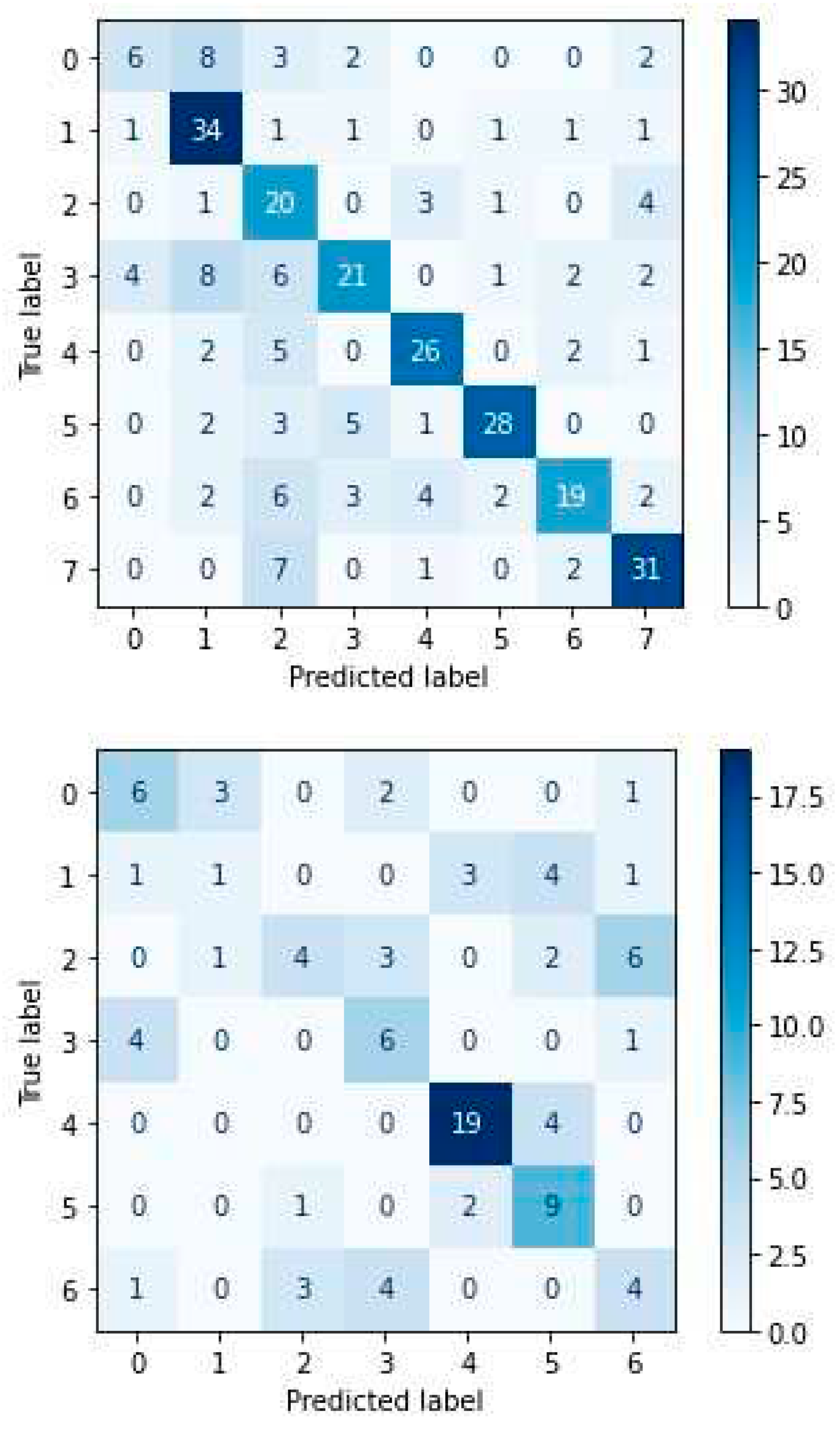
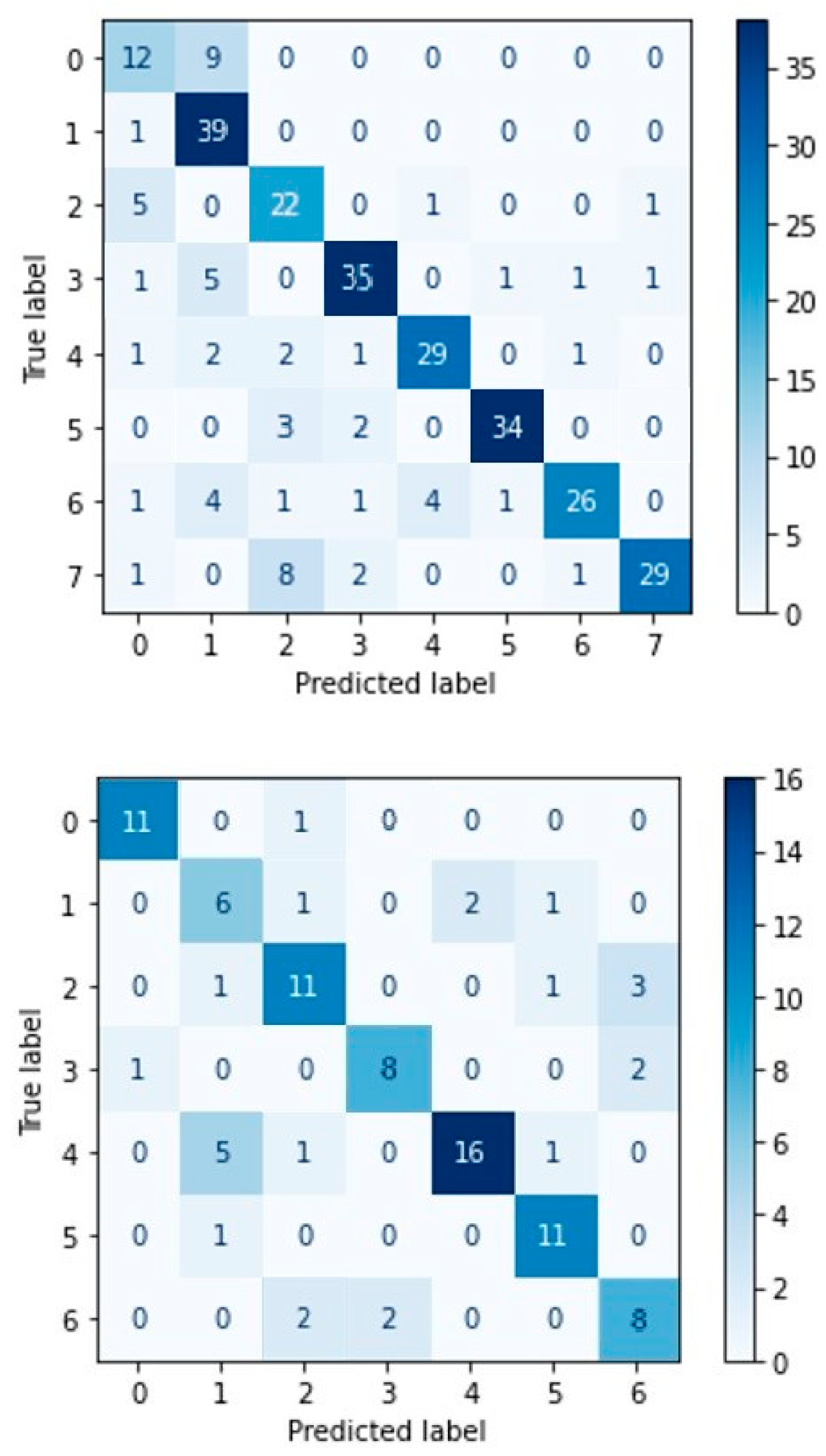
For the six implemented models, the confusion matrices for each of the RAVDESS and SAVEE datasets are presented in this subsection, via the Figures 25 to 30. The confusion matrices, as it is well known, contain information about the success rate of the models’ predictions for each emotion of the selected datasets separately. Table 1 shows the correspondence between the labels in confusion matrices and the two datasets.
From the confusion matrix of DBN for the RAVDESS dataset (Figure 25), we can conclude that the ‘neutral’ and the ‘angry’ emotions of the dataset yields the lowest success rate (0%), as the ‘neutral’ emotion is most often confused with the emotion of ‘calm’ {in 9 out of 20 samples} and the emotion of ‘anger’ is most often confused with the emotion of ‘surprise’ {in 27 out of 36 samples}. In contrast, the emotion of ‘surprise’ receives the best success rate (80.5%) compared to the rest, as it identifies 33 out of 41 samples.
Figure 22. DBN confusion matrices for RAVDESS (left) and SAVEE (right).
Preprints 85403 g025
From the confusion matrix of DBN for the SAVEE dataset (Figure 25), we can conclude that the ‘anger’ emotion of the dataset yields the lowest success rate (25%) by identifying only 3 of the 12 samples, as it confuses most times with the emotion of ‘sadness’ {in 8 out of 12 samples}. In contrast, the emotion of ‘surprise’ receives the best success rate (66.7%) compared to the rest, as it identifies 8 out of 12 samples.
In the confusion matrix of DNN for the RAVDESS dataset (Figure 26), we can see that the ‘neutral’ emotion yields the lowest success rate (14.3%), as it is most often confused with the ‘sad’ emotion {in 5 out of 21 samples} and the emotion of ‘disgust’ {in 5 out of 21 samples}. In contrast, the emotion of ‘surprise’ receives the best success rate (61%) compared to the rest, as it identifies 25 out of 41 samples.
Similarly, in the confusion matrix of DNN for the SAVEE dataset (Figure 26), we can see that the emotion of ‘surprise’ yields the lowest success rate (33.3%) identifying only 4 out of the 12 samples, as it is confused most often with the feeling of ‘fear’ {in 5 out of the 12 samples}. In contrast, the ‘neutral’ emotion receives the best success rate (91.3%) compared to the rest, as it identifies 21 out of 23 samples.
Figure 23. DNN confusion matrices for RAVDESS (left) and SAVEE (right).
Preprints 85403 g026
Figure 24. LSTM network confusion matrices for RAVDESS (left) and SAVEE (right).
Preprints 85403 g027
From the confusion matrix of LSTM for the RAVDESS dataset (Figure 27) we can conclude that the ‘happy’ emotion and the ‘neutral’ emotion of the dataset yield the lowest success rates achieving 44.8% and 66.7%, respectively. This is because the ‘happy’ emotion is most often confused with the emotion of ‘fearful’ {in 7 out of 29 samples} and the ‘neutral’ emotion is sometimes confused with the ‘sad’ emotion {in 3 out of 21 samples}. In contrast, the emotions of ‘calm’ and ‘surprise’ receive the best success rates (80% and 78%), as they identify 32 out of 40 and 32 out of 41 samples, respectively.
From the confusion matrix of LSTM for the SAVEE dataset (Figure 27) we can conclude that the emotion of ‘happiness’ yields the lowest success rate (36.4%) identifying only 4 out of 11 samples, as it is confused several times with both the emotion of ‘anger’ and the emotion of ‘surprise’ {in 3 out of 12 samples for each}. In contrast, the ‘neutral’ emotion receives the optimal success rate (95.6%) compared to the rest, as it identifies 22 of the 23 samples.
Figure 25. LSTM network with attention mechanism confusion matrices for RAVDESS (left) and SAVEE (right).
Preprints 85403 g028
From the confusion matrix of LSTM-ATN for the RAVDESS dataset (Figure 28), we can conclude that the ‘sad’ emotion achieves the lowest success rate (50%) by identifying only 22 out of 44 samples, as it is sometimes confused with the emotion of ‘disgust’ {in 6 out of 44 samples}. In contrast, the ‘calm’ emotion receives the optimal success rate (95%) compared to the rest, as it identifies 38 out of 40 samples.
From the confusion matrix of LSTM-ATN for the SAVEE dataset (Figure 28), we can conclude that the emotion of ‘happiness’ yields the lowest success rate (27.3%) identifying only 3 of the 11 samples, as it is most often confused with the emotion of ‘surprise’ {in 3 out of 11 samples}. In contrast, the neutral emotion receives the optimal success rate (95.6%) compared to the rest, as it identifies 22 out of 23 samples.
Figure 26. CNN network confusion matrices for RAVDESS (left) and SAVEE (right).
Preprints 85403 g029
From the confusion matrix of CNN for the RAVDESS dataset (Figure 29), we can conclude that the ‘neutral’ emotion achieves the lowest success rate (28.6%) by identifying only 6 of the 21 samples, as it is most often confused with the emotion of ‘calm’ {in 8 out of 21 samples}. In contrast, the emotion of ‘calm’ receives the optimal success rate (85%) compared to the rest, as it identifies 34 out of 40 samples.
From the confusion matrix of CNN for the SAVEE dataset (Figure 29), we can conclude that the emotion of ‘disgust’ yields the lowest success rate (10%) by identifying only 1 out of 10 samples, as is confused several times with both the emotion of ‘sadness’ {in 4 out of 10 samples} and the ‘neutral’ emotion {in 3 out of 10 samples}. In contrast, the ‘neutral’ emotion receives the optimal success rate (82.6%) compared to the rest, as it identifies 19 out of 23 samples.
Figure 27. CNN network with attention mechanism confusion matrices for RAVDESS (left) and SAVEE (right).
Preprints 85403 g030
From the confusion matrix of CNN-ATN for the RAVDESS dataset (Figure 30), we can conclude that ‘neutral’ emotion yields the lowest success rate (57%) as it is often confused with the emotion of ‘calm’ {in 9 out of 21 samples}. In contrast, the ‘calm’ emotion receives the optimal success rate (97%) compared to the rest, as it identifies 39 out of 40 samples.
From the confusion matrix of CNN-ATN for the SAVEE dataset (Figure 30), we can conclude that the emotion of ‘disgust’ yields the lowest success rate (60%) by identifying 6 out of 10 samples, as it is confused a few times with the ‘neutral’ emotion {in 2 out of 10 samples}. In contrast, both the emotion of ‘anger’ and the emotion of ‘sadness’ receive the best success rate (91.6%) compared to the rest, as it identifies 11 out of 12 samples.
In conclusion, from all the above we observe that for the RAVDESS base our models can on average perceive more successfully the emotions of ‘calm’ and ‘surprise’, while they find it difficult to determine the ‘neutral’ emotion. This may be due to the fact that in this database there are two basic emotions that approach the ‘neutral’ emotion, one from a negative point of view and the other from a positive point of view, making it difficult to determine the right emotion. Regarding the SAVEE database, we observe that our models can perceive the ‘neutral’ emotion more successfully, as in this database it is unique, while they find it difficult to identify the emotions of ‘happiness’ and ‘disgust’.

4. Discussion

In Table 1, we present the results of the accuracy of prediction of the models we implemented for the RAVDESS and SAVEE databases. Deep Neural Networks (DNNs) are Feedforward Neural Networks and in these networks, information moves in only one direction - forward - from the input nodes, through the hidden nodes and to the output nodes. Deep Belief Networks (DBNs), however, have non-directed connections between some layers, making the topologies of these two models different by definition. Comparing DBN with DNNs, we notice that DBN achieves significantly lower accuracy results for both databases. Concerning DNNs, comparing SDNN with the two LSTM based networks, we observe that the specialization of LSTM in the classification, processing and making predictions on time series data, resulted in a significant improvement of accuracy in the large database (RAVDESS), in contrast to the result in the small database (SAVEE), where there was no improvement (deterioration in the case of simple LSTM). Then, comparing the LSTM networks with the Convolutional Neural Network (CNN), we notice that CNN achieved better results in the (large) RAVDESS database, while in the (small) SAVEE database the results are significantly reduced. This is because the CNN model is designed with a large number of hidden layers (5), which burdens performance, if the amount of data is small, while it improves performance for large amounts of data. The addition of the attention mechanism to the Convolutional Neural Network (as to the LSTM) contributes significantly to the improvement of results for both databases, as the addition of this mechanism equips the neural network with the ability to focus on a subset of inputs/attributes using weights on previous hidden state h ̃_s, thus retaining relevant information from the input side to assist in prediction. So, by combining the information from the input side with those in the current target state h_t as explained in sections 3.4 and 3.6, better prediction rates are achieved.
Table 2. Prediction results of the models in Ravdess and Savee Databases (weighted accuracy).
Models Input Features SAVEE RAVDESS
DBN Average of 40 MFCCs 47.92 32.64
DNN Average of 40 MFCCs 69.79 45.18
LSTM 40 MFCCs 67 70
LSTM-ATN 40 MFCCs 69.79 66
CNN 40 MFCCs 55.2 70.5
CNN-ATN 40 MFCCs 74 77
In the following, we present the comparative study of our proposed method, which is the CNN-ATN, with existing models in the literature that provide state-of-the-art results. The model we propose consists of five convolution layers, each using the batch-normalization technique and the ReLU activation function. The 1st, 2nd and 3rd convolution layers also use the dropout normalization technique to reset 50% of the connections. The result of the last convolutional layer is fed to the attention mechanism, which emphasizes the use of weights in a subset of inputs holding more input information to optimize the performance of the model prediction.
Table 3 presents the performance of the proposed method in comparison with other state-of-the-art proposals, for the SAVEE database. Sivanagaraja et al. [28] proposes a Multi-scale Convolution Network (MCNN) for SER using rawWav to train a DNN, which consists of 3 stages: i) the signal transformation stage, ii) the local convolution stage and iii) the global convolution stage. Latif et al. [29] introduce a Deep Belief Network (DBN) with three RBM layers using the eGeMAPS features set. Fayek et al. [30] developed a Deep Neural Network (DNN) that recognizes emotions from a one second frame of raw speech spectrograms. Chenchah and Lachiri et al [31] utilize the Hidden Markov Model (HMM), categorizing the characteristics exported using Linear Frequency Cepstral Coefficients (LFCCs) and Mel-Frequency Cepstral Coefficients (MFCCs). It is obvious that our method significantly outperforms the other efforts.
Table 4 presents the performance of the proposed method in comparison with other state-of-the-art proposals, for the RAVDESS database. Rajak and Mall [32] present a Convolutional Neural Network (CNN) model, which consists of four one-dimensional (1D) local convolutional filters and receives as input 12 MFCCs, which are extracted from the audio files with a 10ms step of a 50ms window. Also, after the 2nd hidden layer, a max pooling layer is applied. Jalal et al. [7] developed a robust emotion classification method using bidirectional long short-term memory network (BLSTM), CNN and Capsule networks, using a feature vector, which consists of the fundamental frequency (F0), 23-dimensional MFCC and log-energy augmented by delta and delta-delta. The overall network is comprised of two BLSTM layers, 1D conv-capsule layer consisting of capsules and a capsule routing layer. Input layer consists of 70 nodes (length of the feature vector), and each BLSTM hidden layer contains 256 units. The BLSTM deals with the temporal dynamics of the speech signal by effectively representing forward/backward contextual information, while the CNN along with the dynamic routing of the Capsule net learn temporal clusters. Venkataramanan and Rajamohan et al. [33] present a 2Dimensional-CNN with Global Average Pooling, which consists of four layers of convolution with a filter size of 12x12 for the first layer, 7x7 for the second and 3x3 for the other two layers and receives as input Log-Mel Spectrograms. Mohanty et al. [34] developed a Convolutional Neural Network (CNN), which consists of 18 convolution layers and receives as input MFCCs. Huang and Bao et al. [35] utilizes a 2Dimensional-CNN, which consists of 4 convolution layers and after the 2nd and 4th hidden layer, a max pooling layer is applied. This model uses also 13 MFCCs as input. Mustaqeem and Soonil Kwon et al. [8] described a Deep Stride CNN (DSCNN) for SER using Raw Spectrograms for training, which consists of 7 layers of convolution, using the 2x2 stride to sub-sample the size of feature maps, instead of using pooling layers. Issa, Demirci και Yazici [16], in their work, present a model that includes six one-dimensional convolutional layers combined with dropout, batch-normalization, and activation layers. The first layer of their CNN receives 193 × 1 number arrays as input data. The initial layer is composed of 256 filters with the kernel size of 5 × 5 and stride 1, followed by batch normalization and ReLU layer. The next convolutional layer, consisting of 128 filters with the same kernel size and stride, is also using ReLU, and dropout with the rate of 0.1. Next, batch normalization is implemented, feeding its output to the max-pooling layer with a window size of 8. Next, 3 convolution layers with 128 filters of size 5 × 5 are located, two of which are followed by ReLU activation layers and finally by batch normalization, ReLU activation and dropout layer with the rate of 0.2. The final convolutional layer with the same parameters is followed by the flattening layer and dropout with the rate of 0.2. The output of the flattening layer is received by a fully connected layer with 8, 7, or 2 units, depending on the number of predicted classes. After that, batch normalization and softmax activation are applied.

5. Conclusions

The broader literature on Speech Emotion Recognition (SER) systems addresses many challenges in improving emotion recognition accuracy, but also seeks to reduce the computational complexity of models. In recent years, the attention mechanism has begun to be used to improve neural machine translation (NMT) by selectively focusing on parts of the source sentence during translation. However, not many studies have been presented to implement this technique. For this reason, in our study, we propose a model of Convolutional Neural Network with the addition of an attention mechanism, which significantly outperforms other attempts of ours and the state-of-the-art methods, as shown in Table 3 and Table 4, giving the best prediction results: 74% for the SAVEE, and 77% for the RAVDESS databases. This is due to the following reasons. First, for our model we decided to export Mel Frequency Cepstral Coefficients (MFCCs) from the audio data we used for input, as they provide rich feature content from the data in a consistent manner. Another reason is that these coefficients use the Mel scale, which is based on how humans perceive different signal frequencies. Finally, the addition of the attention mechanism to the simple CNN enabled our model to focus on the parts of the audio input which contain more emotional information, than parts where the speaker does not say something or words that are not emotionally intense, helping to further improve the ability to predict emotion.
Our future work concerns, testing our model on other databases, and try different modern deep learning architectures like Transformers [36].

Author Contributions

Conceptualization, I.P. and K.M.; methodology, I.P.; software, K.M. and I.P.; validation, K.M.; investigation, I.P..; data curation, K.M.; writing—original draft preparation, I.P. and K.M..; writing—review and editing, I.H. supervision, I.H.; All authors have read and agreed to the published version of the manuscript.

Funding

This research received no external funding.

Conflicts of Interest

The authors declare no conflict of interest.

Notes

1
2
3

References

  1. Wang, X.; Zhang, Y.; Yu, S.; Liu, X.; Yuan, Y.; Wang, F. E-learning recommendation framework based on deep learning. In Proceedings of the 2017 IEEE International Conference on Systems, Man, and Cybernetics (SMC); 2017; pp. 455–460. [Google Scholar] [CrossRef]
  2. Jelena Gligorijevic, Djordje Gligorijevic, Martin Pavlovski, Elizabeth Milkovits, Lucas Glass, Kevin Grier, Praveen Vankireddy, Zoran Obradovic. Optimizing clinical trials recruitment via deep learning. Journal of the American Medical Informatics Association 2019, 26, 1195–1202. [Google Scholar] [CrossRef]
  3. Davatzikos, C.; Ruparel, K.; Fan, Y.; Shen, D.; Acharyya, M.; Loughead, J.; Gur, R.; Langleben, D.D. Classifying spatial patterns of brain activity with machine learning methods: Application to lie detection. NeuroImage 2005, 28, 663–668. [Google Scholar] [CrossRef]
  4. Justesen, N.; Bontrager, P.; Togelius, J.; Risi, S. Deep Learning for Video Game Playing. IEEE Transactions on Games 2020, 12, 1–20. [Google Scholar] [CrossRef]
  5. Lavrentyeva, G.; Novoselov, S.; Malykh, E.; Kozlov, A.; Kudashev, O.; Shchemelinin, V. Audio Replay Attack Detection with Deep Learning Frameworks. Proc. Interspeech 2017, 82–86. [Google Scholar] [CrossRef]
  6. Uchechukwu Ajuzieogu. The Role of AI In Modern Computing and Education”, Computer Education Seminar 2019, UNN, A seminar approach to understanding the underlying principles of AI and its relevance to Education, in the 21st Century, 2019.
  7. Jalal, M.A.; Loweimi, E.; Moore, R.K.; Hain, T. Learning Temporal Clusters Using Capsule Routing for Speech Emotion Recognition. Proc. Interspeech 2019, 1701–1705. [Google Scholar] [CrossRef]
  8. Mustaqeem; Kwon, S. A CNN-Assisted Enhanced Audio Signal Processing for Speech Emotion Recognition. Sensors 2020, 20, 183. [Google Scholar]
  9. Singh, Y.B.; Goel, S. A systematic literature review of speech emotion recognition approaches. Neurocomputing 2022, 492, 245–263. [Google Scholar] [CrossRef]
  10. Wani, T.M.; Gunawan, T.S.; Qadri, S.A.A.; Kartiwi, M.; Ambikairajah, E. A comprehensive review of speech emotion recognition systems. IEEE access 2021, 9, 47795–47814. [Google Scholar] [CrossRef]
  11. Khalil, R.A.; Jones, E.; Babar, M.I.; Jan, T.; Zafar, M.H.; Alhussain, T. Speech emotion recognition using deep learning techniques: A review. IEEE Access 2019, 7, 117327–117345. [Google Scholar] [CrossRef]
  12. Abbaschian, B.J.; Sierra-Sosa, D.; Elmaghraby, A. Deep learning techniques for speech emotion recognition, from databases to models. Sensors 2021, 21, 1249. [Google Scholar] [CrossRef]
  13. Wen, G.; Li, H.; Huang, J.; Li, D.; Xun, E. Random Deep Belief Networks for Recognizing Emotions from Speech Signals. Computational Intelligence and Neuroscience 2017, 2017, 1945630. [Google Scholar] [CrossRef]
  14. Badshah, A.M.; Ahmad, J.; Rahim, N.; Baik, S.W. Speech Emotion Recognition from Spectrograms with Deep Convolutional Neural Network. In Proceedings of the 2017 International Conference on Platform Technology and Service (PlatCon); 2017; pp. 1–5. [Google Scholar] [CrossRef]
  15. Zhao, J.; Mao, X.; Chen, L. Speech emotion recognition using deep 1D & 2D CNN LSTM networks. Biomed. Signal Process. Control. 2019, 47, 312–323. [Google Scholar]
  16. Lee, C.; Song, K.Y.; Jeong, J.; Choi, W.Y. Convolutional Attention Networks for Multimodal Emotion Recognition from Speech and Text Data. arXiv 2019, arXiv:1805.06606. [Google Scholar]
  17. Tang, D.; Zeng, J.; Li, M. An End-to-End Deep Learning Framework for Speech Emotion Recognition of Atypical Individuals. Proc. Interspeech 2018, 162–166. [Google Scholar] [CrossRef]
  18. Chen, M.; He, X.; Yang, J.; Zhang, H. 3-D Convolutional Recurrent Neural Networks With Attention Model for Speech Emotion Recognition. IEEE Signal Processing Letters 2018, 25, 1440–1444. [Google Scholar] [CrossRef]
  19. Li, P.; Song, Y.; Mcloughlin, I.; Guo, W.; Dai, L. An Attention Pooling Based Representation Learning Method for Speech Emotion Recognition. Interspeech 2018. [Google Scholar]
  20. Jiang, W.; Wang, Z.; Jin, J.S.; Han, X.; Li, C. Speech Emotion Recognition with Heterogeneous Feature Unification of Deep Neural Network. Sensors 2019, 19, 2730. [Google Scholar] [CrossRef]
  21. Huang, K.; Wu, C.; Hong, Q.; Su, M.; Chen, Y. Speech Emotion Recognition Using Deep Neural Network Considering Verbal and Nonverbal Speech Sounds. In Proceedings of the ICASSP 2019 - 2019 IEEE International Conference on Acoustics, Speech and Signal Processing (ICASSP), Brighton, United Kingdom; 2019; pp. 5866–5870. [Google Scholar] [CrossRef]
  22. Issa, D.; Demirci, M.; Yazici, A. Speech emotion recognition with deep convolutional neural networks. Biomedical Signal Processing and Control 2020, 59, 101894. [Google Scholar] [CrossRef]
  23. Makhmudov, F.; Kutlimuratov, A.; Akhmedov, F.; Abdallah, M.S.; Cho, Y.I. Modeling Speech Emotion Recognition via Attention-Oriented Parallel CNN Encoders. Electronics 2022, 11, 4047. [Google Scholar] [CrossRef]
  24. Abdul, Z.K.; Al-Talabani, A.K. Mel Frequency Cepstral Coefficient and its applications: A Review. IEEE Access 2022. [Google Scholar] [CrossRef]
  25. Luong, M.T.; Pham, H.; Manning, C.D. Effective Approaches to Attention-based Neural Machine Translation. arXiv 2015, arXiv:1508.04025. [Google Scholar]
  26. Jackson, P.; Haq, S. Surrey Audio-Visual Expressed Emotion (SAVEE) database. 2011. Available online: http://kahlan.eps.surrey.ac.uk/savee/Database.html.
  27. Livingstone, S.R.; Russo, F.A. The Ryerson Audio-Visual Database of Emotional Speech and Song (RAVDESS): A dynamic, multimodal set of facial and vocal expressions in North American English. PLoS ONE 2018, 13, e0196391. [Google Scholar] [CrossRef] [PubMed]
  28. Sivanagaraja, T.; Ho, M.K.; Khong, A.W.H.; Wang, Y. End-to-end speech emotion recognition using multi-scale convolution networks. In Proceedings of the 2017 Asia-Pacific Signal and Information Processing Association Annual Summit and Conference (APSIPA ASC), Kuala Lumpur; 2017; pp. 189–192. [Google Scholar] [CrossRef]
  29. Latif, S.; Rana, R.; Younis, S.; Qadir, J.; Epps, J. Transfer Learning for Improving Speech Emotion Classification Accuracy. arXiv 2018, arXiv:1801.06353. [Google Scholar]
  30. HFayek, M.; Lech, M.; Cavedon, L. Towards real-time Speech Emotion Recognition using deep neural networks. In Proceedings of the 2015 9th International Conference on Signal Processing and Communication Systems (ICSPCS), Cairns, QLD; 2015; pp. 1–5. [Google Scholar] [CrossRef]
  31. Chenchah, F.; Lachiri, Z. Acoustic Emotion Recognition Using Linear and Nonlinear Cepstral Coefficients. International Journal of Advanced Computer Science and Applications (IJACSA) 2015, 6. [Google Scholar] [CrossRef]
  32. Rajak, R.; Mall, R. Emotion recognition from audio, dimensional and discrete categorization using CNNs. In Proceedings of theTENCON 2019 - 2019 IEEE Region 10 Conference (TENCON), Kochi, India; 2019; pp. 301–305. [Google Scholar] [CrossRef]
  33. Venkataramanan, K.; Rajamohan, H.R. Emotion Recognition from Speech. arXiv 2019, arXiv:1912.10458. [Google Scholar]
  34. Mohanty, H.; Budhvant, S.; Gawde, P.; Shelke, M. Implementation of Mood Detection through Voice Analysis using Librosa and CNN. In Proceedings of the International Research Journal of Engineering and Technology (IRJET), Thane, Maharashtra, India, 6 June 2020; pp. 5876–5879. [Google Scholar]
  35. Huang, A.; Bao, P. Human Vocal Sentiment Analysis. arXiv 2019, arXiv:1905.08632. [Google Scholar]
  36. Wagner, J.; et al. Dawn of the Transformer Era in Speech Emotion Recognition: Closing the Valence Gap. IEEE Transactions on Pattern Analysis and Machine Intelligence 2023, 45, 10745–10759. [Google Scholar] [CrossRef]
Table 1. Correspondence between the emotion labels and the emotions in the two datasets.
Label of Emotion Emotion in SAVEE Emotion in RAVDESS
[0] anger neutral
[1] disgust calm
[2] fear happy
[3] happiness sad
[4] neutral angry
[5] sadness fearful
[6] surprise disgust
[7] - surprise
Table 3. Comparison with the previous works using SAVEE Database.
Models Input Features SAVEE - Test accuracy (%)
MCNN Sivanagaraja [28] rawWav 50.28
DBN Latif [29] eGeMAPS 56.76
DNN Fayek, Lech and Cavedon [30] Spectrogram 59.7
HMM Chenchah and Lachiri [31] LFCCs/MFCCs 45/61.25
Proposed method MFCCs 74
Table 4. Comparison with the previous works using RAVDESS Database.
Models Input Features RAVDESS - Test accuracy (%)
CNN Rajak and Mall [32] MFCCs 47.92
BLSTM-CNN-Capsule Network Jalal [7] F0, MFCCs, Log Spectrogram augmented by delta and delta-delta 56.2
2D CNN with Global Avg Pool Venkataramanan
and Rajamohan [33]
Log Mel Spectrogram 69.79
CNN Mohanty [34] MFCCs 67
CNN Huang and Bao [35] MFCCs 69.79
DSCNN Mustaqeem and Soonil Kwon [8] Raw Spectrograms / Clean Spectrograms 68 / 80
1D CNN Issa, Demicri and Yazici [22] MFCCs, chromagram and Mel-Spectrogram 71.61
Proposed method MFCCs 77
Disclaimer/Publisher’s Note: The statements, opinions and data contained in all publications are solely those of the individual author(s) and contributor(s) and not of MDPI and/or the editor(s). MDPI and/or the editor(s) disclaim responsibility for any injury to people or property resulting from any ideas, methods, instructions or products referred to in the content.
Copyright: This open access article is published under a Creative Commons CC BY 4.0 license, which permit the free download, distribution, and reuse, provided that the author and preprint are cited in any reuse.
Prerpints.org logo

Preprints.org is a free preprint server supported by MDPI in Basel, Switzerland.

Subscribe

© 2024 MDPI (Basel, Switzerland) unless otherwise stated