Mean-Field Analysis with Random Perturbations to Detect Gliders in Cellular Automata

Preprint

Article

Mean-Field Analysis with Random Perturbations to Detect Gliders in Cellular Automata

Altmetrics

Downloads

112

Views

Comments

A peer-reviewed article of this preprint also exists.

Juan Carlos Seck-Tuoh-Mora^*

Joselito Medina-Marin

Norberto Hernández-Romero

,Genaro J. Martínez

Juan Carlos Seck-Tuoh-Mora^*

Joselito Medina-Marin

Norberto Hernández-Romero

,Genaro J. Martínez

This version is not peer-reviewed

Submitted:

15 September 2023

Posted:

19 September 2023

You are already at the latest version

Alerts

Abstract

Cellular automata are mathematical models that represent systems with complex behavior through simple interactions between their individual elements. These models can be used to study unconventional computational systems and complexity. One notable aspect of cellular automata is their ability to create structures known as gliders, which move in a regular pattern to represent the manipulation of information. This paper introduces the modification of mean-field theory applied to cellular automata, using random perturbations based on the system’s evolution rule. The original aspect of this approach is that the perturbation factor is tailored to the nature of the rule, altering the behavior of the mean-field polynomials. By combining the properties of both the original and perturbed polynomials, it is possible to detect when a cellular automaton is more likely to generate gliders without having to run evolutions of the system.This methodology is a useful approach to finding more examples of cellular automata that exhibit complex behavior. We start by examining elementary cellular automata, then move on to examples of automata that can generate gliders with more states. To illustrate the results of this methodology, we provide evolution examples of the detected automata.

Keywords:

Subject: Computer Science and Mathematics - Computer Science

1. Introduction

The study of self-reproducing systems capable of self-repairing and carrying out computational processes without the need for a central control unit led to the emergence of cellular automata (CAs). This work was pioneered by John von Neumann and Stanislaw Ulam, and later edited and completed by Arthur W. Burks in [1].

After its inception, cellular automata studies have had numerous facets, primarily benefiting from their easy computational implementation and simple mathematical specifications. This has enabled their modification, adaptation, and application in exploring theoretical concepts like new computational paradigms [2], system reversibility [3], and comprehending how complexity arises from homogeneous elements’ local interaction in a system [4]. These are just a few of the many applications of cellular automata.

The study of cellular automata has experienced significant growth, particularly in the creation of self-reproducing systems from Von Neumann’s original 29-state model. The LIFE cellular automaton [5,6] has sparked further investigation into the interaction of structures moving in a fixed background and the creation of complex systems using only a two-state automaton in two dimensions. Additionally, the analysis of elementary cellular automata (ECAs) has been a breakthrough in complexity analysis.

Despite having the simplest computational implementation, they are capable of generating complex behaviors, as noted in [7,8]. ECAs computational capabilities are studied in detail in [9], and in [10] it is shown that ECA rule 110 can implement a universal computing system.

Various works have tackled the issue of detecting gliders in cellular automata (CAs). One such method is presented in [11], which automatically filters CA spatiotemporal patterns to identify gliders and related emergent configurations. Another study [12] comprehensively analyzes gliders in ECA rule 54. In [13], a rigorous upper bound on the number of distinct products that gliders can generate is established, particularly for ECA rule 54. Meanwhile, [14] presents a method that uses genetic programming to search for new cellular automata that can perform computational tasks using gliders. Two variants of particle kinetic models based on CAs describing two glider species are discussed in [15]. In [16], Ameyalli’s rule, a new two-dimensional CA, is described, featuring an emergent glider gun used to construct logic gates for logical universality. A new system mixing a CA and a genetic algorithm, showing interesting behaviors and glider production, is presented in [17]. Isotropic CAs capable of producing glider-gun and eater dynamics are explained in [18]. In [19], a new approach to duplicating information flows in two-dimensional CAs based on glider-specific collisions capable of simulating logic gates is proposed. In [20], a simple triangular partitioned CA with triangular cells, each divided into three parts, capable of producing gliders is studied. New tools are introduced in [21] to study self-organization in a family of CAs containing gliders and coalescence properties according to some initial shift-ergodic measure using the limiting measure to describe the asymptotic behavior of the CA. Finally, [22] investigates the use of ECAs and shifting spatiotemporal dynamics of automata enriching cells with memory to produce complex behaviors.

Research in the detection of cellular automata with complex behaviors is a thriving area of study. The focus is mainly on ECAs, particular cases, and extended models of CAs. However, most of these works use a posteriori point of view, which means they take a sample of CA evolutions to determine if it can generate gliders in a fixed or periodic background.

In this study, we analyze a cellular automaton using classical mean-field theory tools and random perturbations to determine if it can generate gliders in a periodic background without the need for observing multiple evolutions of the automaton. The evolutions presented in the study serve to validate the complex dynamics identified by the methodology outlined in this research.

The original part of the paper lies in the utilization of classical mean-field theory polynomials, and the addition of random perturbations applied to them. These perturbations are determined by observing the behavior of the CA evolution rule and noting whether it generates a higher frequency of certain types of neighborhoods over others.

The density of a CA states can be estimated using classical and perturbed mean-field polynomials, which can then be used to identify high and low classes of densities linked to every state. If the classes identified by the classical polynomials differ from those identified by the perturbed polynomials, it suggests a critical behavior in the CA dynamics. This means that the automaton can have relevant changes in its density of states during its evolution, with the high classes representing a periodic background and the low classes identifying moving structures (or "gliders") within that background.

This study involves simulating ECAs and one-dimensional CAs with a neighborhood size of two cells, which extends the findings of the study. By utilizing this broad approach, the suggested methodology can be utilized for other CAs with a wider range of states.

The contribution of this study lies in proposing a new methodology capable of detecting mobile structures in a periodic background of a CA with a neighborhood size of 2. The methodology does not require calculating the CA evolutions in advance. This methodology is first applied for the case of ECAs simulated with four-state CAs and two-cell neighborhoods, then applied to CAs with up to 9 states.

The paper is structured as follows: In Section 2, a one-dimensional CA, an ECA, and the simulation of all CA using neighborhoods of only two cells are formally described. Section 3 defines mean-field polynomials for CA with neighborhood size of 2 and applies these polynomials to predict the dynamic behavior of the densities of states for the ECA rule 110. Section 4 explains how a random perturbation is applied to the mean-field polynomials, depending on the evolution rule’s tendency to favor the formation of one neighborhood over others. With this, a methodology is specified to detect CAs forming gliders in a periodic background, based on the analysis of the evolution rule using the classical and perturbed mean-field polynomials. In Section 5, the methodology is applied to CAs, presenting evolutions of CAs capable of generating gliders. Section 6 applies this methodology to CAs with a larger number of states, showing examples of CAs capable of producing complex behaviors. Finally, Section 7 provides the conclusions of this work.

2. Preliminaries of Cellular Automata

This paper will focus on the study of cellular automata in one dimension. A cellular automaton (CA) is defined by three main components: a set of states S, a neighborhood radius r, and an evolution rule, denoted as

φ : S^{2 r + 1} \to S

. The CA takes an initial configuration or condition

c^{0} : Z_{m} \to S

, where

c^{0}

is a one-dimensional array consisting of m cells, with each cell assigned a state from S. The cell at position i is represented by

c_{i}^{0}

To understand the dynamics of cellular automata (CA), a block of states is defined as

w_{i} = {c_{i - r}^{0} \dots c_{i + r}^{0}}

, which consists of r neighboring cells both to the left and right of each

c_{i}^{0}

. Using this information, the new state

c_{i}^{1}

is determined through

φ (w_{i})

. To ensure that the number of cells in

c^{1}

is m, periodic boundary conditions are applied. The evolution rule

φ

creates a global mapping

Φ : c^{j} \to c^{j + 1}

between configurations, which defines the overall dynamics of the CA.An elementary cellular automaton (ECA) is the simplest type of CA capable of generating complex behaviors. In this case,

| S | = 2

and

r = 1

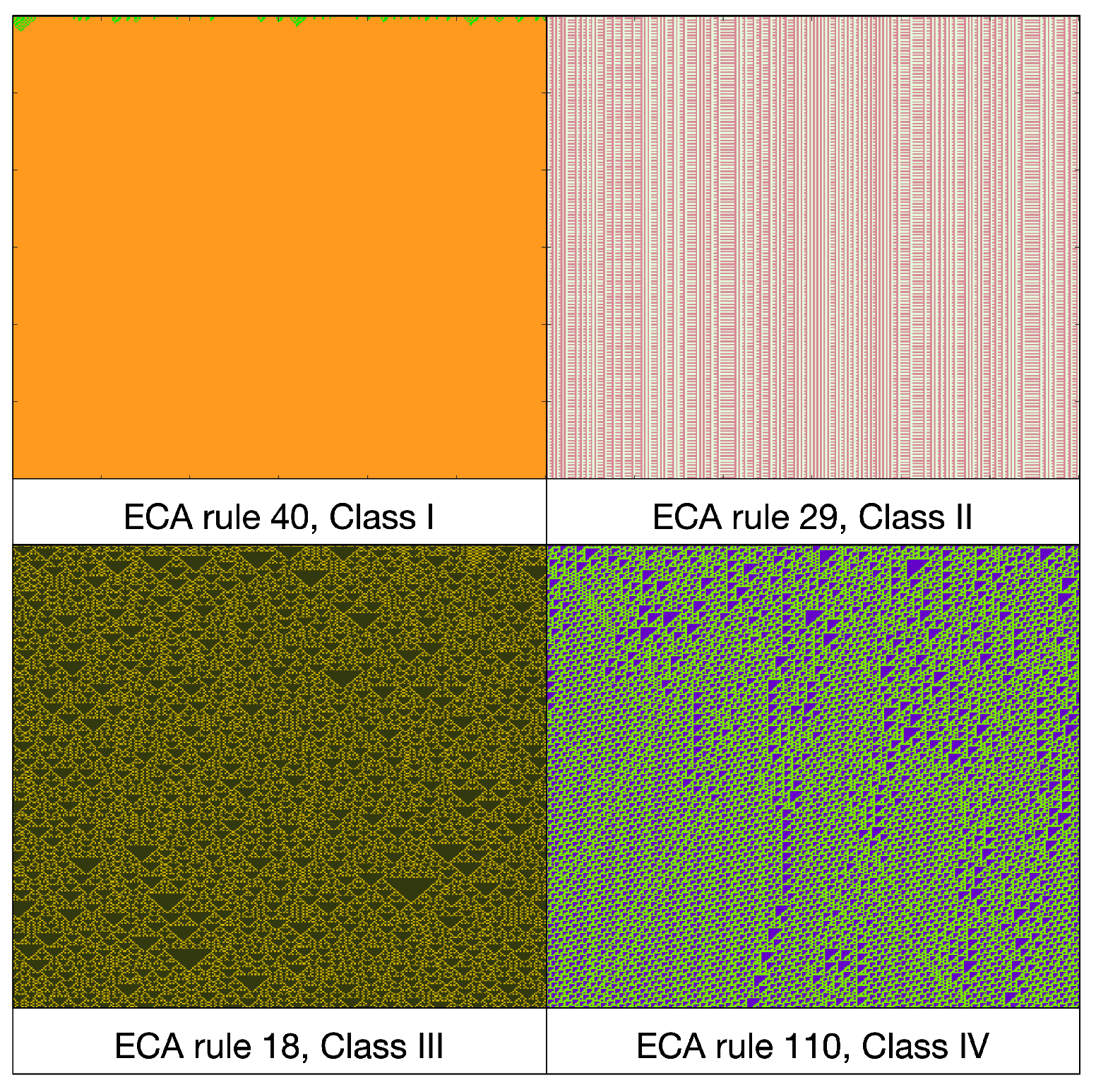
ECAs are widely studied due to their simplicity and the variety of dynamics they can produce. These dynamics can range from fixed or periodic global states to chaotic and complex behaviors. Various classifications have been proposed to categorize the dynamics of ECAs. The most well-known classification is the one by Wolfram, which defines four classes based on the observed dynamics of ECAs. These classes include Class I, which generates a fixed global state, Class II, which produces a periodic global state, Class III, which exhibits chaotic behavior, and Class IV, which results in complex evolutions [23]. To illustrate each class, Figure 1 displays an example of each class using

m = 300

and 300 evolutions.

Complexity in cellular automata (CAs) is a blend of order and chaos. The automaton’s evolution creates a stable or repeating background with moving structures called gliders. These gliders interact with one another, either cancelling each other out, creating a different type of glider, or remaining preserved. Complex cellular automata (CAs) rely on a delicate balance between two defining characteristics: periodicity and chaos. This balance ensures that neither characteristic becomes dominant. Gliders can represent information in these CAs, and logical operators can be implemented through their interactions to enforce a computing process. One-dimensional CAs have a unique property where any CA can be simulated using another CA with a neighborhood size 2, even if it requires a significant increase in the number of states.

For a CA with a neighborhood radius of r,

| S |

states and

φ : S^{2 r + 1} \to S

evolution rule, extending the action of

φ

S^{n}

produces sequences in

S^{n - 2 r}

for

n > 2 r

. By extending the definition of

φ

, one can map

φ : S^{2 r + 2 r} \to S^{2 r}

. Therefore, we can use a new set of states W with

| S^{2 r} |

states, and

φ : W^{2} \to W

to simulate a CA with

| S |

states and a neighborhood size of 2r+1. It is customary that the evolution of each neighborhood is centered on the following configuration for the new automaton.

While this process has an exponential growth rate that depends on r in the number of new set states, it is advantageous because the results obtained using CAs with a neighborhood size of 2 can be generalized to all other cases.

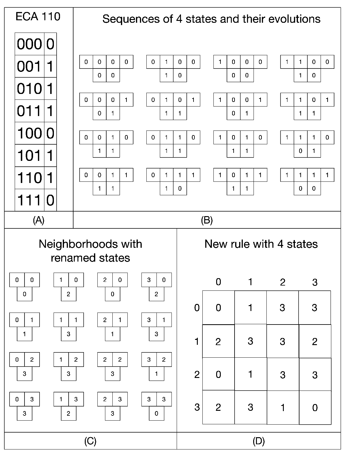
To simulate ECAs, we can use 4 state CAs. We’ll use the example of ECA rule 110 shown in Figure 2. In (A), we see the evolution rule of ECA 110. In (B), we observe the sequences of 4 states and their evolutions using

φ

. In (C), we’ve renamed each sequence in

S^{2 r}

with its decimal value, resulting in a new state set

W = {0, \dots, 3}

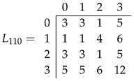
. Finally, in (D), we’ve reordered the new evolution rule in matrix form, where the row and column indices are the states of W, and each entry

(w_{1}, w_{2})

shows the evolution of each sequence

w_{1} w_{2} \in W^{2}

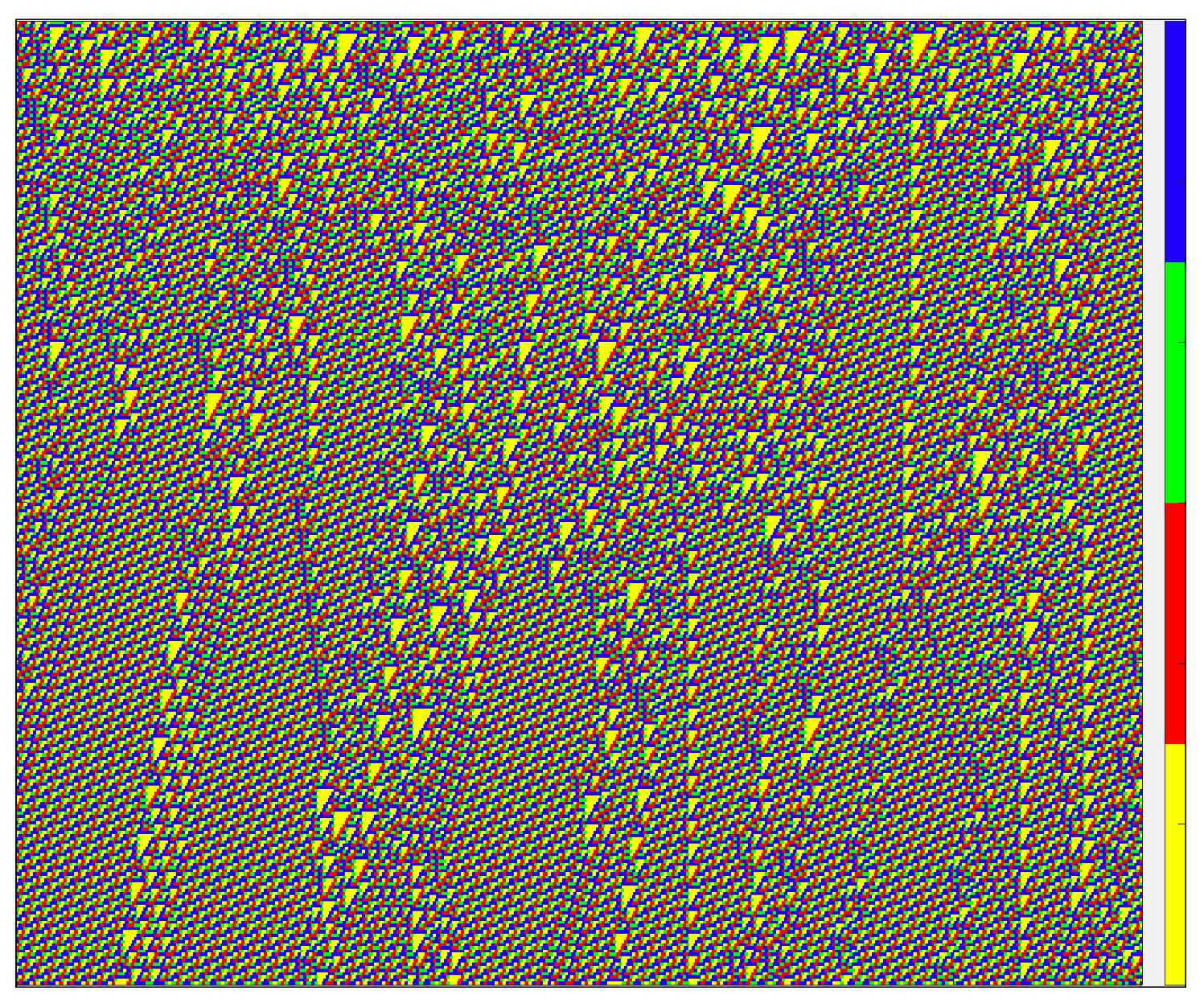
Figure 3 shows an evolution of the CA that simulates the ECA rule 110.

3. Mean-Field Analysis

One method of studying the dynamic behavior of a CA is by using mean-field theory. This involves utilizing polynomials that describe how the densities of CA states change based on previous densities, in an iterative manner [24,25]. This approach is advantageous due to its ease of implementation, as the polynomials only require initial values to calculate subsequent densities. However, a disadvantage is that the polynomials tend to quickly converge to an average density, losing the small fluctuations that can occur in the CA evolutions and may indicate complex dynamics.

Here is an example of how to define mean-field polynomials for a CA with a neighborhood size of 2 and

| S | = 4

. To define the polynomial for each density state, we’ll start by looking at the set

X = S^{2}

of all possible neighborhoods such as

{00, 01, 02, 03, \dots, 33}

. For

s \in S

, let

d_{s}^{0}

be the initial density of state s in

c^{0}

, which can be found experimentally as:

d_{s}^{0} = \frac{\sum_{i = 1}^{m} α (c_{i}^{0}, s)}{m}

(1)

where

α (c_{i}^{0}, s) = \{\begin{matrix} 1 & i f f c_{i}^{0} = s \\ 0 & i n o t h e r c a s e s \end{matrix}

(2)

Using the neighborhoods in X, we will have 4 mean-field polynomials; one for each state, whose general definition is:

p (d_{s}^{k + 1}) = \sum_{x \in X} β (x, s) d_{x}^{k}

(3)

with

β (x, s) = \{\begin{matrix} 1 & i f f φ (x) = s \\ 0 & i n o t h e r c a s e s \end{matrix}

(4)

where

k \geq 0

denotes the iteration step of the polynomial and

d_{x}^{k}

is the estimated density of the neighborhood x in the

c^{k}

configuration. Assuming that initially

c^{0}

is defined randomly, one can assume independence in the occurrence of each state in

c^{0}

, so that for

x = s_{i} s_{j}

d_{x}^{0} = d_{s_{i}}^{0} d_{s_{j}}^{0}

, with

0 \leq i, j \leq 3

and

s_{i} \in S

. This assumption is repeated for subsequent values of k.

The mean-field polynomials satisfy that

\sum_{s \in S} p (d_{s}^{k}) = 1

\forall k \geq 0

. It is important to note that the independence of state occurrences in a configuration is justified when it is randomly defined. Polynomials are useful for calculating a decent approximation of density behavior, especially when configurations have a larger number of cells. However, this definition of polynomials may not fully capture the behavior of densities, especially in complex CA.

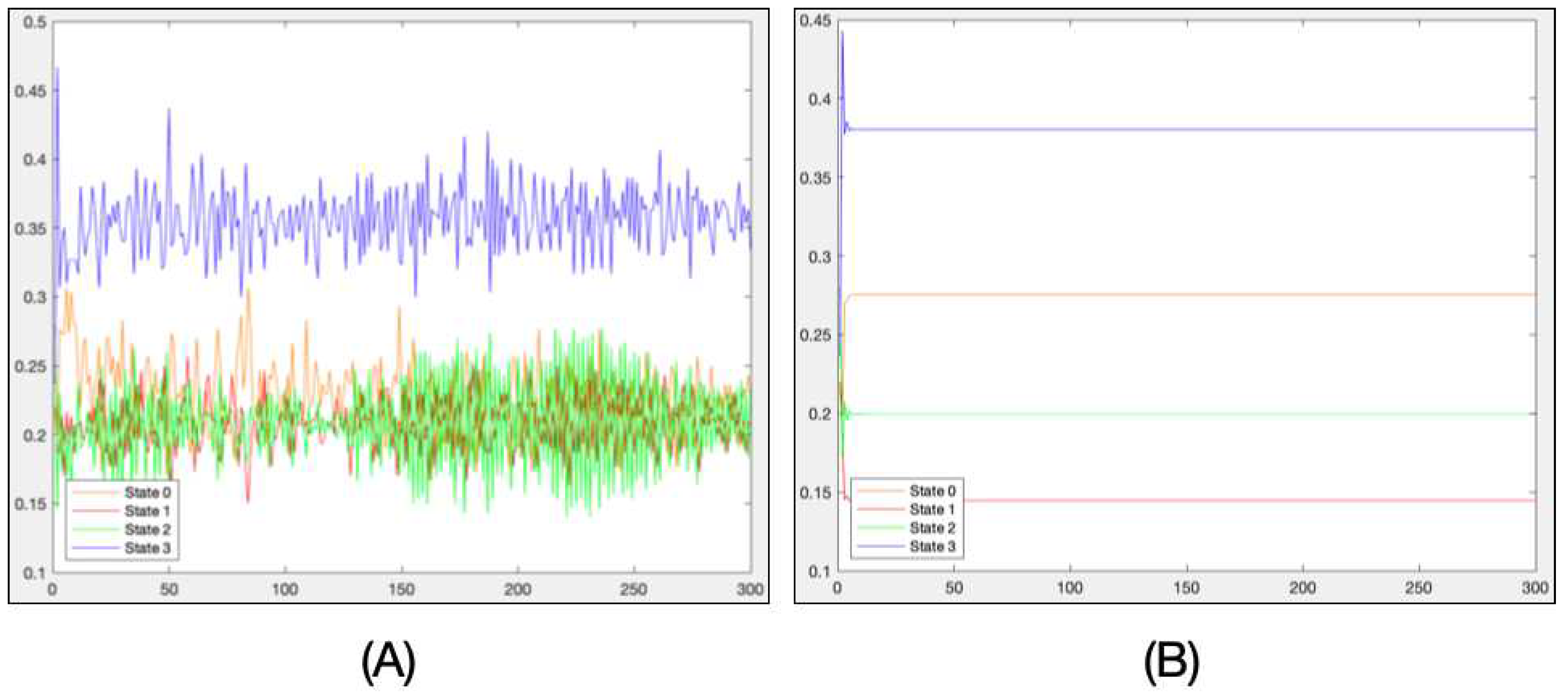
For instance, consider the CA of 4 states presented in Figure 2 that emulates the ECA rule 110. In (A) of Figure 4, we can observe the experimental density of the CA when

m = 300

and 300 evolutions. Additionally, (B) shows the corresponding approximation calculated by the mean-field polynomials.

We can observe from Figure 4 that while the mean-field polynomials defined in Eq. 3 provide a good approximation to the mean density, they quickly reach a fixed value. In part (B), the highest estimated density belongs to the 3 state, followed by the density of the 1 state, while the other states have lower estimated densities. However, experimentally, the densities of the states 1 to 3 are similar.

This reveals that mean-field polynomials can provide initial information to identify a complex CA. States with higher densities work to create periodic backgrounds, while the remaining states form gliders. Thus, a first filter to determine if a CA is complex is to check its estimated densities. If the densities are not very high (less than

0.5

) and are heterogeneous, meaning they have two distinct classes of states, with one having higher densities and the other having slight but not negligible densities (greater than

0.1

), then the CA may be able to yield complex behaviors.

4. Random Perturbation of Mean-Field Analysis

In the previous section, it was noted that the estimation of mean-field polynomials needs to be more accurate for determining the densities of states in complex CAs. Although the estimation yields two states with higher density, the experimental part shows a dominant density and others with a similar, lower density. To complement this analysis and identify whether a CA can generate complex behaviors, random perturbations are applied to the mean-field polynomials. This is done to test the robustness of the polynomials in maintaining their high and low-density classes. If the density estimations remain stable when small random perturbations are applied, it would indicate that the polynomials define very stable dynamics.

However, if small random perturbations cause a significant change in the polynomial estimation, such as the high-density classes being different in the original polynomials than in the perturbed polynomials, then the density dynamics are sensitive to these perturbations. This is when we can detect CAs with complex behavior.

The random perturbation of signals is an area of active research in various fields such as mathematics and computer science. Examples of its application include linear signal tracking [26], global optimization metaheuristics [27,28], neural network synchronization [29], optimal control for stochastic dynamical systems [30], analyzing the transient dynamics of predator-prey systems [31], asymptotic covariance estimation [32] and studying the numerical approximation of partial differential equations [33]. Notably, to our knowledge, this type of analysis has not been applied to detect complex dynamics in CAs.

The mean-field polynomials with random perturbations will be defined as follows.

d_{s}^{k + 1} = q (d_{s}^{k}) = \sum_{x \in X} γ g (x) d_{x}^{k}

(5)

where

g (x)

is a factor representing the tendency the evolution rule

φ

has to produce the neighborhood x in a CA, and

γ

is a random number between 0 and

γ_{max}

Random perturbation of signals has been an active field of research in several mathematics and computer science areas. For example, for the linear tracking of signals [26], for global optimization metaheuristics [27,28], for neural network synchronization [29], for optimal control for a stochastic dynamical system [30], for analyzing the transient dynamics of a predator-prey system [31], for the asymptotic covariance estimation [32], for the study of the numerical approximation of partial differential equations [33] to mention some representative works. However, to our knowledge, this type of analysis has yet to be applied to detect complex dynamics in CAs.

The factor

g (x)

depends directly on

φ

and is calculated as follows.

For each element x in the set X, count the number of ancestral sequences $l_{x}$ . Here, $l_{x}$ refers to the number of sequences w in $S^{3}$ such that $φ (w) = x$ .
For each $x \in X$ , the average number of ancestors can be calculated as ${| S |}^{3} / {| S |}^{2} = | S |$ . If $l_{x} > | S |$ , it is assumed that the $φ$ evolution rule promotes the emergence of the x-neighborhood, while if $l_{x} < | S |$ , it is said to discourage it.
We define a tendency matrix M of order $| S | \times | S |$ such that each entry $m_{i, j} = \frac{l_{x} - | S |}{| S |}$ for all $i, j \in S$ and $x = i j$ .
Finally $g (x) = m_{i, j}$ for $x = i j$ .

The idea is that

g (x)

is zero if the neighborhood x has an average number of ancestors, and otherwise it has a positive or negative value if the evolution rule does or does not favor its formation based on the average value.

Finally, the random value

γ

is a weighting factor for applying

g (x)

to each density in Eq. 5; in this study, we take

γ = 0.75

The concept behind

g (x)

is to assign a value of zero to the neighborhood x if it has an average number of ancestors. However, if the evolution rule favors or does not favor its formation based on the average value,

g (x)

will have a positive or negative value.

To apply

g (x)

to each density in Equation 5, a random value called

γ

is used as a weighting factor. In this study, we have chosen to use

γ = 0.75

In order to maintain that

\sum_{s \in S} q (d_{s}^{k}) = 1

\forall k \geq 0

after applying the perturbations

γ g (x)

, we take the difference

e = \frac{1 - \sum_{s \in S} q (d_{s}^{k})}{| S |}

(6)

We update

d_{s}^{k} = d_{s}^{k} + e

\forall s \in S

. After perturbing and normalizing the polynomials, we can recalculate the densities

d_{s}

through an iterative process. This results in two sets of densities: the first set obtained using the classical polynomials (refer to Eq. 3), and the second set estimated using equations 5 and 6.

We will be utilizing both types of polynomials to detect CAs that have gliders in a periodic background. To do this, we will classify the states as either belonging to a high-estimated density class or a low-estimated density class.

For each $s \in S$ we compute the average densities $\bar{d_{s}}$ after m iterations.
The highest density ${\bar{d}}_{m a x}$ defines the first state s in the high-density $C_{h i g h}$ class.
For $δ = {\bar{d}}_{m a x} - ϵ$ the remaining densities $\bar{d_{s}} > = δ$ define the remaining states in $C_{h i g h}$ .
The rest of the states define the class $C_{l o w}$ with low densities.

In this work, we will set

ϵ

to 0.15 for differences between

C_{h i g h}

and

C_{l o w}

. Using classical and perturbed polynomials, we get two pairs of classes:

C_{h i g h}^{c}

and

C_{l o w}^{c}

from classical polynomials, and

C_{h i g h}^{p}

and

C_{l o w}^{p}

from perturbed polynomials. These classes will determine the parameters needed to identify potential CAs yielding gliders.

The maximum densities in $C_{h i g h}^{c}$ and $C_{h i g h}^{p}$ must not exceed $0.5$ .
$| C_{h i g h}^{c} | \neq | C_{h i g h}^{p} |$ .
$| C_{l o w}^{c} | > 0$ and $| C_{l o w}^{p} | > 0$ .

5. Experiments with ECAs

To test the methodology explained in the previous section, we first took all ECAs from rule 0 to rule 255. Each ECA is first simulated with a CA of 4 states and 2 neighborhood size, and on this rule, the mean-field polynomials, both classical and randomly perturbed, were applied depending on the rule trends.

For the case of the 110 rule, the 64 sequences of 3 states and their evolutions were taken. Let us use

L_{110}

as the matrix showing the number of ancestor sequences of each x neighborhood where each entry

(i, j)

L_{110}

is equal to

l_{x}

for

x = i j

In order to test the methodology described in the previous section, we examined all ECAs from rule 0 to rule 255. Each ECA was simulated using a CA with 4 states and a neighborhood size of 2. Mean-field polynomials, both classical and randomly perturbed, were then applied based on the trends of each rule.

For the specific case of rule 110, we analyzed the 64 sequences of 3 states and their corresponding evolutions. We used a matrix called

L_{1} 10

to represent the number of ancestor sequences for each x neighborhood, where each entry

(i, j)

L_{1} 10

is equal to

l_{x}

for

x = i j

(7)

Taking

L_{110}

, the matrix

M_{110}

is obtained by taking

\frac{L_{110} - 4}{4}

(8)

Using the elements of matrix

M_{110}

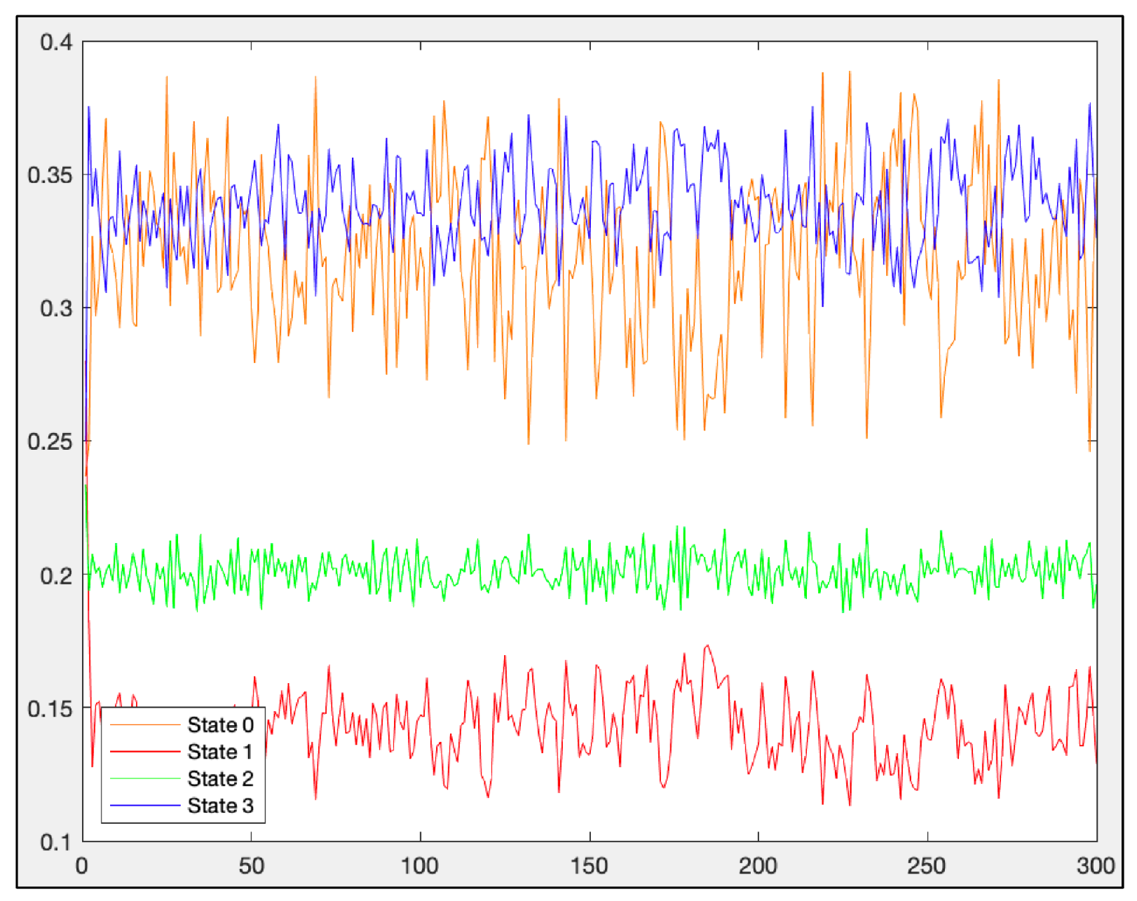
, we apply random perturbations to mean-field polynomials in Eq. 5 and normalize them with Eq. 6. Figure 5 illustrates the behavior of estimated densities under this scheme.

Referring to Figure 4-(B) and Figure 5, and following the class detection method explained in Section 4, we can determine that

C_{h i g h}^{c} = {3}

C_{l o w}^{c} = {0, 1, 2}

C_{h i g h}^{p} = {0, 3}

C_{l o w}^{p} = {1, 2}

. These classes indicate that mean-field polynomials display critical behavior when subjected to random perturbations, suggesting their ability to generate gliders during their evolution.

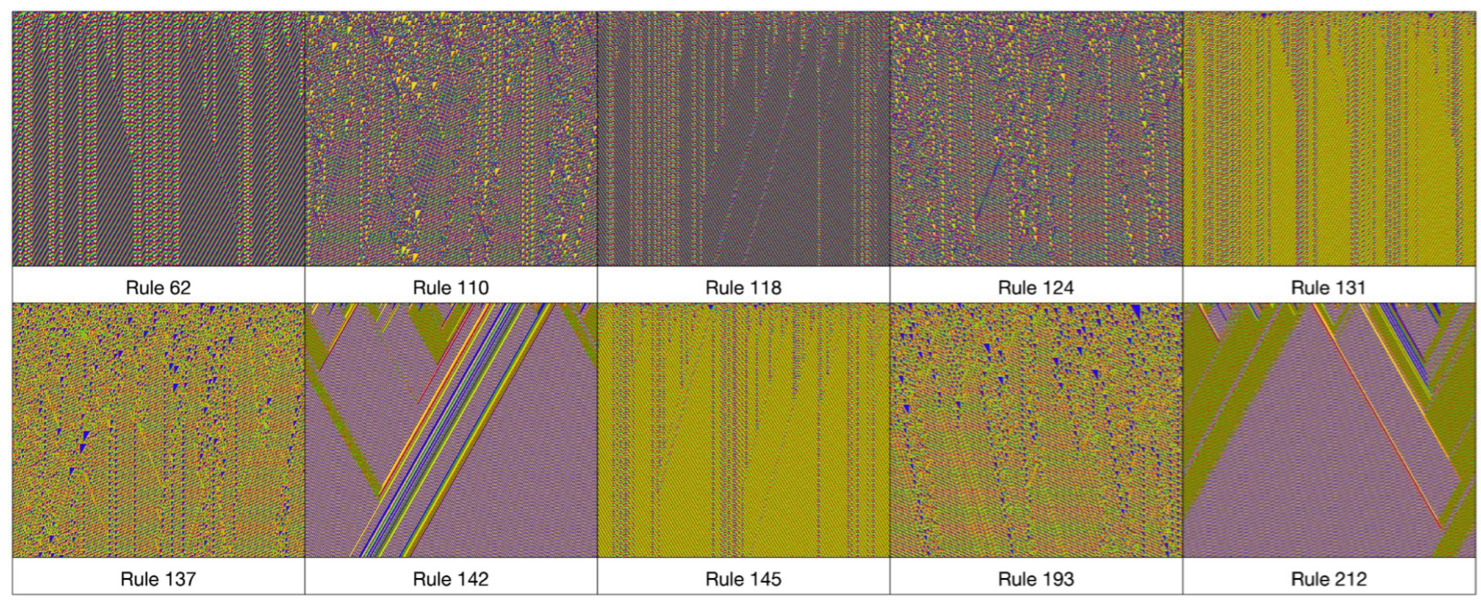
Figure 6 illustrates the ECAs identified as capable of generating gliders in a periodic background. This was determined by simulating them as 4-state CAs and using the criteria specified in the final part of Section 4, which involves classical and randomly perturbed mean-field polynomials.

6. Experiments with a higher number of states

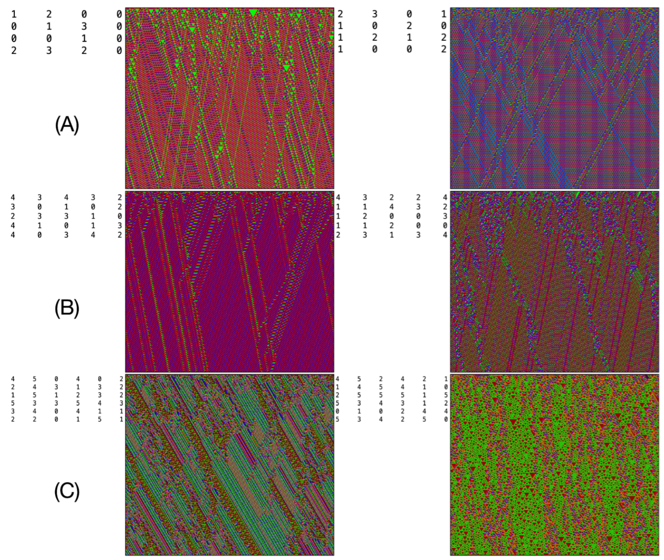
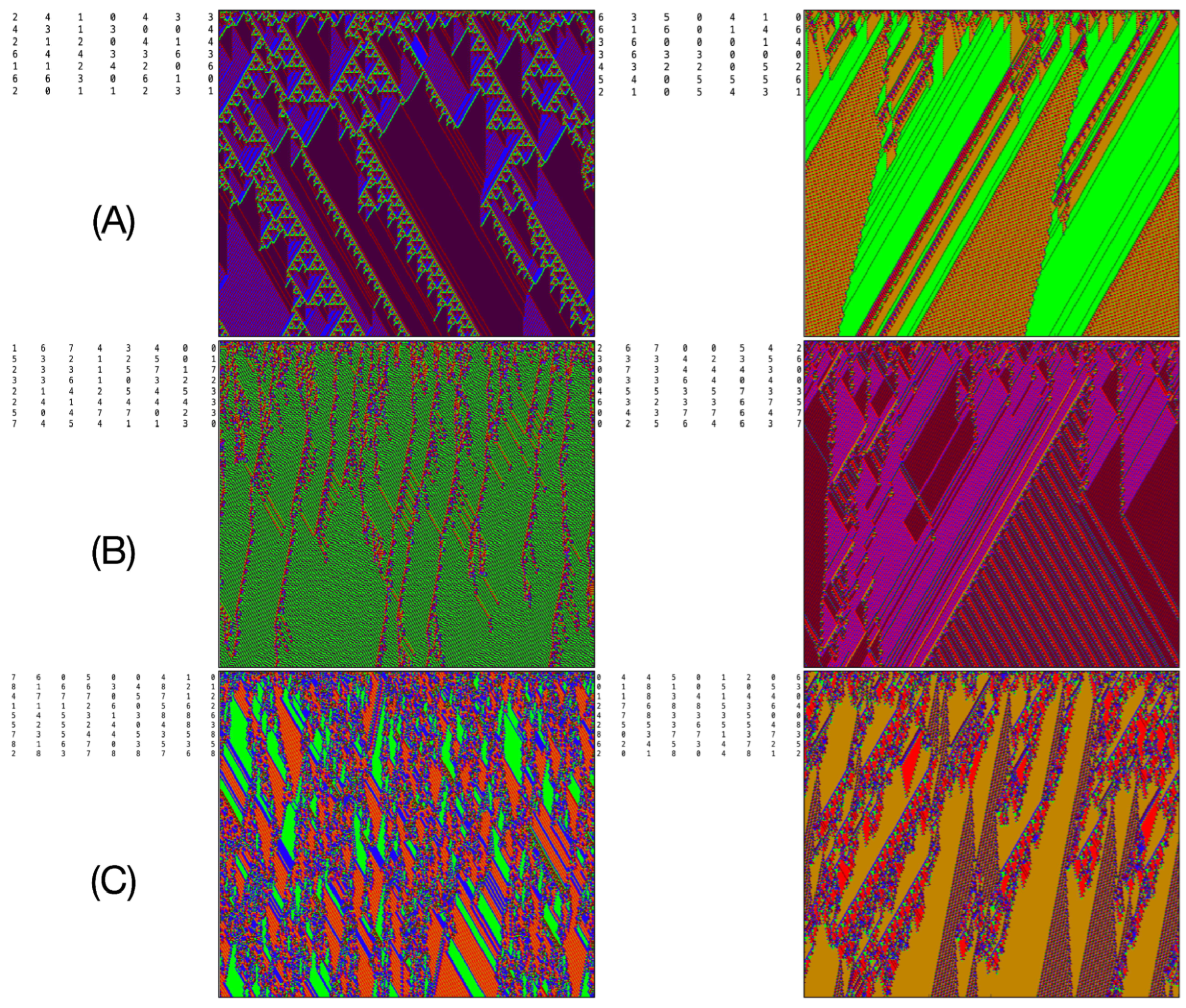
We modified the method to identify now CAs that can generate gliders with 4 to 9 states and a neighborhood size 2. Figure 7 displays two examples for each case, including 4 states (A), 5 states (B), and 6 states (C). The matrix form of the evolution rule is also provided for each case.

Figure 8 shows examples for 7, 8, and 9 states ((A), (B), and (C) respectively), including their associated evolution rules.

7. Conclusions

In this paper, a straightforward approach to detecting CAs that can produce gliders in a periodic background using mean-field classical polynomials and randomly perturbed polynomials has been presented. The trends of the evolution rule to produce each neighborhood have been considered.

The significant contribution of this work is the detection of CAs capable of generating gliders without the need to observe the automaton’s evolutions but by analyzing its evolution rule. The methodology has been applied to simulated ECAs with 4-state CAs and then extended to CAs with 4 to 9 states, revealing some fascinating specimens that can generate gliders in a periodic background.

However, this methodology needs further refinement to detect CAs with more complex behavior accurately. For instance, for CAs with a quasi-periodic background, as in the case of the ECA rule 54.

Future work that may arise from this research includes the application of other ways of extending mean-field polynomials to account for a more significant number of densities. Working on the state independence assumption in a different way, such as using Bayesian probability. Measuring the tendency of the evolution rule to generate some state sequences with higher probability than others in different ways. Or using deep learning computational tools that better model the production of states and sequences of a CA.

Author Contributions

Conceptualization, J.C.S.-T.-M. and G.J.M.; methodology, J.C.S.-T.-M. and N.H.-R.; validation, J.M.-M., N.H.-R. and J.C.S.-T.-M.; formal analysis, J.C.S.-T.-M. and G.J.M.; investigation, J.M.-M., N.H.-R. and J.C.S.-T.-M.; resources, J.M.-M. and J.C.S.-T.-M.; writing—original draft preparation, J.M.-M., N.H.-R. and J.C.S.-T.-M.; writing—review and editing, J.C.S.-T.-M. and G.J.M. visualization, J.C.S.-T.-M. and J.M.M.; supervision, G.J.M.; funding acquisition, J.M.-M. and J.C.S.-T.-M. All authors have read and agreed to the published version of the manuscript.

Funding

This study was supported by the Autonomous University of Hidalgo (UAEH) and the National Council for Science and Technology (CONACYT) with projects numbers CB-2017-2018-A1-S-43008 and F003/320109.

Institutional Review Board Statement

Not applicable.

Informed Consent Statement

Not applicable.

Data Availability Statement

Not applicable.

Conflicts of Interest

The authors declare that they have no known competing financial interest or personal relationships that could have appeared to influence the work reported in this paper.

Abbreviations

CA	Cellular automata
ECA	Elementary cellular automata

References

Burks, A.W. Theory of self-reproducing automata; University of Illinois Press US, 1966.
Adamatzky, A. Collision-based computing; Springer Science & Business Media, 2012.
Kari, J. Reversible cellular automata: from fundamental classical results to recent developments. New Generation Computing 2018, 36, 145–172. [Google Scholar] [CrossRef]
Ilachinski, A. Cellular automata: a discrete universe; World Scientific Publishing Company, 2001.
Conway, J.; others. The game of life. Scientific American 1970, 223, 4. [Google Scholar]
Adamatzky, A. Game of life cellular automata; Vol. 1, Springer, 2010.
Voorhees, B.H. Computational analysis of one-dimensional cellular automata; Vol. 15, World Scientific, 1996.
McIntosh, H.V. One dimensional cellular automata; Luniver Press, 2009.
Wolfram, S. ; others. A new kind of science; Vol. 5,Wolfram media Champaign, IL, 2002.
Cook, M.; others. Universality in elementary cellular automata. Complex systems 2004, 15, 1–40. [Google Scholar]
Wuensche, A. Classifying cellular automata automatically: Finding gliders, filtering, and relating space-time patterns, attractor basins, and the Z parameter. Complexity 1999, 4, 47–66. [Google Scholar] [CrossRef]
Martínez, G.J.; Adamatzky, A.; McIntosh, H.V. Phenomenology of glider collisions in cellular automaton Rule 54 and associated logical gates. Chaos, Solitons & Fractals 2006, 28, 100–111. [Google Scholar]
Hordijk, W.; Shalizi, C.R.; Crutchfield, J.P. Upper bound on the products of particle interactions in cellular automata. Physica D: Nonlinear Phenomena 2001, 154, 240–258. [Google Scholar] [CrossRef]
Sapin, E.; Bailleux, O.; Jean-Jacques, C. Research of a cellular automaton simulating logic gates by evolutionary algorithms. European Conference on Genetic Programming. Springer, 2003, pp. 414–423.
Prosen, T. On two non-ergodic reversible cellular automata, one classical, the other quantum. Entropy 2023, 25, 739. [Google Scholar] [CrossRef]
Gómez Soto, J.; Wuensche, A. The Ameyalli-Rule: Logical Universality in a 2D Cellular Automaton. Journal of Cellular Automata 2022, 16, 197. [Google Scholar]
Cerruti, U.; Dutto, S.; Murru, N. A symbiosis between cellular automata and genetic algorithms. Chaos, Solitons & Fractals 2020, 134, 109719. [Google Scholar]
Wuensche, A.; Gómez Soto, J. Isotropic Cellular Automata: the DDLab iso-rule paradigm. Journal of Cellular Automata 2020, 15, 439. [Google Scholar]
Sapin, E. Automatization of universal cellular automaton discoveries: a new approach to stream duplication. Complex Systems 2020, 29, 77–86. [Google Scholar] [CrossRef]
Morita, K. A universal non-conservative reversible elementary triangular partitioned cellular automaton that shows complex behavior. Natural Computing 2019, 18, 413–428. [Google Scholar] [CrossRef]
Hellouin de Menibus, B.; Sablik, M. Self-organisation in cellular automata with coalescent particles: qualitative and quantitative approaches. Journal of Statistical Physics 2017, 167, 1180–1220. [Google Scholar] [CrossRef]
Martinez, G.J.; Adamatzky, A.; Alonso-Sanz, R. Designing complex dynamics in cellular automata with memory. International Journal of Bifurcation and Chaos 2013, 23, 1330035. [Google Scholar] [CrossRef]
Wolfram, S. Computation theory of cellular automata. Communications in mathematical physics 1984, 96, 15–57. [Google Scholar] [CrossRef]
Gutowitz, H.A.; Victor, J.D.; Knight, B.W. Local structure theory for cellular automata. Physica D: Nonlinear Phenomena 1987, 28, 18–48. [Google Scholar] [CrossRef]
McIntosh, H.V. Wolfram’s class IV automata and a good life. Physica D: Nonlinear Phenomena 1990, 45, 105–121. [Google Scholar] [CrossRef]
Guo, B.Z.; Han, J.Q.; Xi, F.B. Linear tracking-differentiator and application to online estimation of the frequency of a sinusoidal signal with random noise perturbation. International Journal of Systems Science 2002, 33, 351–358. [Google Scholar] [CrossRef]
MARYAK, J.L.; CHIN, D.C. Global Random Optimization by Simultaneous Perturbation Stochastic Approximation. IEEE transactions on automatic control 2008, 53, 780–783. [Google Scholar] [CrossRef]
Sun, L.; Chen, S.; Xu, J.; Tian, Y.; others. Improved monarch butterfly optimization algorithm based on opposition-based learning and random local perturbation. Complexity 2019, 2019. [Google Scholar] [CrossRef]
Ge, C.; Chang, C.; Liu, Y.; Hua, C. Dynamic Event-triggered Exponential Synchronization for Neural Networks With Random Controller Gain Perturbations. International Journal of Control, Automation and Systems 2023, 1–11. [Google Scholar] [CrossRef]
Lukashiv, T.; Litvinchuk, Y.; Malyk, I.V.; Golebiewska, A.; Nazarov, P.V. Stabilization of stochastic dynamical systems of a random structure with Markov switches and Poisson perturbations. Mathematics 2023, 11, 582. [Google Scholar] [CrossRef]
Tan, J.; Wang, W.; Feng, J. Transient Dynamics Analysis of a Predator-Prey System with Square Root Functional Responses and Random Perturbation. Mathematics 2022, 10, 4087. [Google Scholar] [CrossRef]
Zhou, J.; Lan, W.; Wang, H. Asymptotic covariance estimation by Gaussian random perturbation. Computational Statistics & Data Analysis 2022, 171, 107459. [Google Scholar]
Guignard, D. Partial differential equations with random input data: A perturbation approach. Archives of Computational Methods in Engineering 2019, 26, 1313–1377. [Google Scholar] [CrossRef]

Figure 1. Examples of dynamic behaviors in ECAs

Figure 2. Simulation of the ECA rule 110 with another CA with 4 states

Figure 3. Evolution of the 4-state CA simulating the ECA rule 110

Figure 4. Density of states calculated experimentally and by means of the mean-field polynomials

Figure 5. Estimated densities for ECA rule 110 by randomly perturbed mean-field polynomials according to Eqs. 5 and 6

Figure 6. ECAs detected with the ability to generate gliders

Figure 7. CAs with 4 to 6 states and neighborhood size 2 able to generate gliders

Figure 8. CAs with 7 to 9 states and neighborhood size 2 able to generate gliders

Disclaimer/Publisher’s Note: The statements, opinions and data contained in all publications are solely those of the individual author(s) and contributor(s) and not of MDPI and/or the editor(s). MDPI and/or the editor(s) disclaim responsibility for any injury to people or property resulting from any ideas, methods, instructions or products referred to in the content.

© 2023 by the authors. Licensee MDPI, Basel, Switzerland. This article is an open access article distributed under the terms and conditions of the Creative Commons Attribution (CC BY) license (http://creativecommons.org/licenses/by/4.0/).

Copyright: This open access article is published under a Creative Commons CC BY 4.0 license, which permit the free download, distribution, and reuse, provided that the author and preprint are cited in any reuse.

MDPI Initiatives

Important Links

Choose an area of interest and we will send you notifications of new preprints at your preferred frequency.

Disclaimer

Mean-Field Analysis with Random Perturbations to Detect Gliders in Cellular Automata

Abstract

1. Introduction

2. Preliminaries of Cellular Automata

3. Mean-Field Analysis

4. Random Perturbation of Mean-Field Analysis

5. Experiments with ECAs

6. Experiments with a higher number of states

7. Conclusions

Author Contributions

Funding

Institutional Review Board Statement

Informed Consent Statement

Data Availability Statement

Conflicts of Interest

Abbreviations

References

MDPI Initiatives

Important Links

Subscribe