1. Introduction
One of the main problems when carrying out a flight with a drone is to be successful in the initial ascension maneuver since these are the most critical phases in a flight, whether manned or not, and where adverse conditions as external disturbances can act more unpredictably, being able to generate accidents when executing these maneuvers. Neural Networks have proven useful to solve and improve flight control tasks. Therefore, in this work, and through the use of Artificial Intelligence, a vertical ascension of a UAV in adverse conditions is performed while using Reinforcement Learning [
1] and the Deep Q-Network (DQN) algorithm [
2].
Although external forces can severely affect the trajectory of a drone’s initial lift and stability, this disturbance is often not considered in training sessions carried out in simulators. For this reason, an external disturbance system was implemented in the Gazebo simulator [
3] to be able to carry out the drone training.
For this, a drone was trained with the aim of reaching a certain height of 6 meters inside the simulator. Six meters is a distance that can be considered sufficient in a vertical elevation of a drone to observe how the UAV is affected by external disturbances and to train it with a sufficiently wide sample.
Reinforcement learning was used for the elevation maneuver, employing the DQN algorithm so that it was able to find the best solution while it was being affected by these external forces, based on the knowledge that it acquired during the initial exploration in its training.
For this, the reward function [
4] was tuned, which would model the behavior of the drone in order to reduce both the oscillation in the orientation and to be able to increase its stability, as well as for its position when taking off. We needed to reward the agent positively or negatively to promote a behavior that optimized the ascension maneuver under these conditions.
This work has demonstrated how a drone can face adverse conditions, such as coping with external disturbances while performing a vertical elevation by using DQN, and how, throughout the training, it has been able to increase its stability against external wind forces of up to 24 mph speed.
2. Background
Flight control with an autonomous vehicle is a complex task. One of the main reasons is the limitations in sensor technology that lead to problems when measuring wind turbulence [
5]. To build an accurate model within a simulated real-world environment, it is essential to employ a paradigm capable of handling continuous control tasks, such as Reinforcement Learning. This learning method does not make any preconceived assumptions about the dynamics of the aircraft or the environmental conditions. Therefore, it is capable of creating optimal control policies.
However, not all reinforcement learning approaches are equally helpful when facing a non-discrete environment. Within reinforcement learning, some algorithms obtain the best results when performing actions in a manageable environment, but become useless when trying to perform a discretization of a real environment, since it faces the problem known as “Curse of dimensionality” [
6]. In other words, when we face a simulation of a real and continuous environment, such as a vertical lift with unpredictable forces applied, the dimensionality of the possible states becomes so large that it is almost impossible for the model to identify or correlate any patterns.
Additional research has introduced an innovative adaptive neural network (NN) zeta-backstepping control method tailored for uncertain nonlinear systems, facilitating the damping ratio adjustment. This method incorporates a second-order Lyapunov function to ensure system stability [
7]. In addition to this, alternative control strategies, including an observer-based adaptive fuzzy finite-time attitude control for UAV maneuvering, have been developed [
8].
Furthermore, certain proposals advocate for sliding mode-based control systems, specifically employing the Proportional Integral Derivative sliding surface control with backstepping (hybrid control). This approach aims to enhance quadcopter flight tracking performance during take-off and soft landing in challenging environmental conditions characterized by disruptions and strong winds [
9].
Lastly, robust adaptive control has demonstrated its effectiveness and remains a viable solution. It continues to be employed, featuring adaptive control schemes designed to tackle uncertain parameters [
10].
Regarding the use of artificial intelligence, some authors have made recent use of machine learning to predict future disturbances by comparing prediction accuracy [
11] between a KNN algorithm (K-closest neighbor) and an LSTM (long-term memory) network. Other authors explore different methods for attitude control [
11] by using the PPO2 algorithm [
12] (Reinforcement algorithm within the category policy optimization), and synthesizing the neural network on a physical controller, significantly reducing the reality gap (jump between the simulator and the real world).
On the other hand, authors have used Deep reinforcement learning along with visual hardware input implementations (cameras) and ground markers to locate the drone in space through the camera and ease maneuvers [
13]. For this, they have used markers on the ground to guarantee a straight vertical elevation, using the camera as an input sensor to verify the correct performance. After that, they check the efficiency of 3 algorithms in the same maneuver: DQN, Double DQN, and Dueling DQN.
Lastly, several authors [
14] propose solutions for obstacle avoidance in the AirSim environment [
15]. As for external disturbances implementations, some experiments use Deep reinforcement learning strategies to land a drone in a moving platform while being pushed by an always front-facing force [
16] and ultimately use the camera to recognize the platform and approach it.
However, most of these experiments in the field of AI have been conducted in environments free of external disturbances, and those that have taken such forces into account have only addressed the problem of landing with a consistent and unidirectional external force. In the experiments that were analyzed as state-of-the-art, the external disturbance exerted a constant force and originated from virtually the same direction, resulting in no unpredictable conditions encountered by the agent.
This work aims to introduce a neural network capable of coping with erratic external disturbances in terms of intensity, duration, and direction, all within the simulator during a vertical elevation. This would present a challenge in training from the very first episode and ultimately enable the formation of a drone model capable of responding to these situations in a real environment as they might occur.
For this, our methodology encompasses several key steps. First, we present the mathematical model of a quadcopter. Subsequently, we create a simulated environment using ROS (Robot Operating System) and Gazebo to replicate real-world conditions. We model wind effects to challenge the take-off maneuver to introduce additional complexity. For the control and adaptation of the quadcopter in the face of these external forces, we employ a reinforcement learning algorithm, specifically DQN (Deep Q-Network), chosen for its capability to handle dynamic environments. We then initiate training, continually refining the reward function until convergence is achieved, ensuring a successful take-off at a height of 6 meters. Finally, we present the observations gleaned from this training process and discuss the conclusions derived from our experimentation.
3. Mathematical Modeling of Quadcopter Dynamics
The quadcopter is assumed to be a rigid body, allowing the use of the Newton-Euler equations to describe its dynamics [
17]. If we consider a body-fixed frame, in the absence of any external disturbances, the forces required for the acceleration of mass
and the centrifugal force
are equal to gravity
and the total thrust of the rotors
:
In the inertial frame, the centrifugal force is nullified. Thus, only the gravitational force and the magnitude and direction of the thrust contribute to the acceleration of the quadcopter:
Where
and
G is the gravity vector. This model is only suitable for ideal conditions, where external disturbances are not considered. One of the most relevant disturbances is the aerodynamic drag effect. Drag force is defined by the well-known relation:
where
is the air density,
v is the aerodynamic speed,
S is the lifting body surface, and
the coefficient of drag. To consider these effects, and additional term must be added to Equation
2:
where
is a diagonal matrix containing the drag force coefficients (
), and
is a vector denoting dynamic pressure. A more detailed description of this aerodynamic model implementation can be found in the literature [
18].
In the body frame, the angular acceleration of the inertia
, the centripetal forces
, and the gyroscopic forces
are equal to the external torque
:
The angular accelerations in the inertial frame are obtained from the body frame accelerations using the inverse transformation matrix
and its time derivative:
Where are the Euler angles, are the angular velocities, and W is the transformation matrix.
4. Methodology
Once the mathematical model has been briefly described, we will develop a methodology to train, test and evaluate the algorithm. The proposed goal was to achieve a vertical elevation up to 6 meters high and maintain the drone stable in its vertical rise while experiencing external disturbances of up to 24 mph speed.
4.1. Possible actions
The first step is to define the actions that can be carried out by the drone. By collectively or individually increasing or decreasing the angular velocity of each of the four rotors, the quadcopter is capable of performing a total of 8 actions, including: going up, going down, Yaw +, Yaw -, Pitch +, Pitch -, Roll +, and Roll -.
Video showing the possible actions to perform
4.2. Environment
After defining the actions, we have to set up the simulation environment. We started using Ubuntu on a clean machine. For the communication with the agent that trains in the Gazebo environment we employed Mavros [
19], a package that allowed us to either publish (send) or subscribe (receive) orders or topics to the PX4 [
20] flight controller that our agent incorporated.
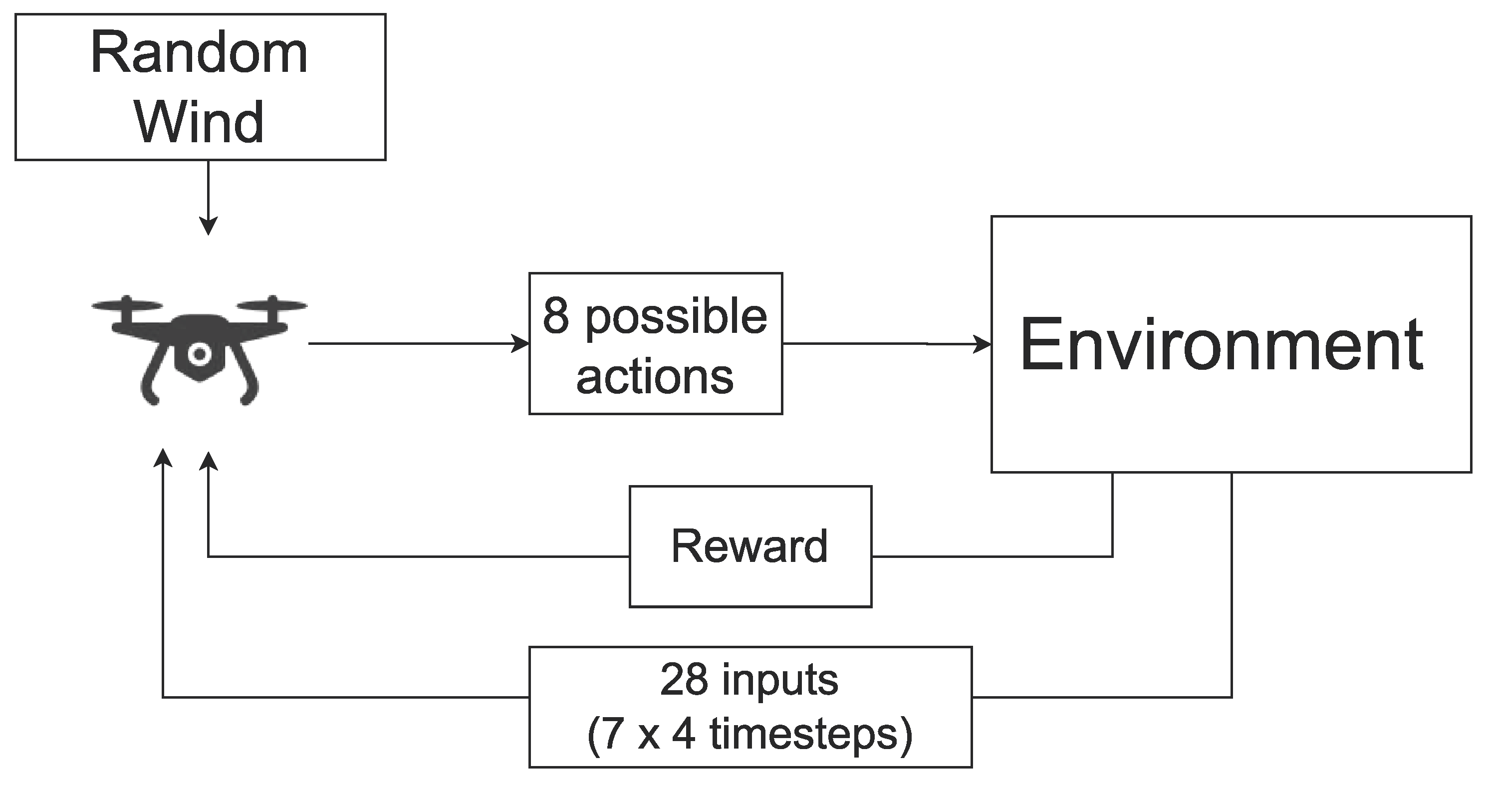
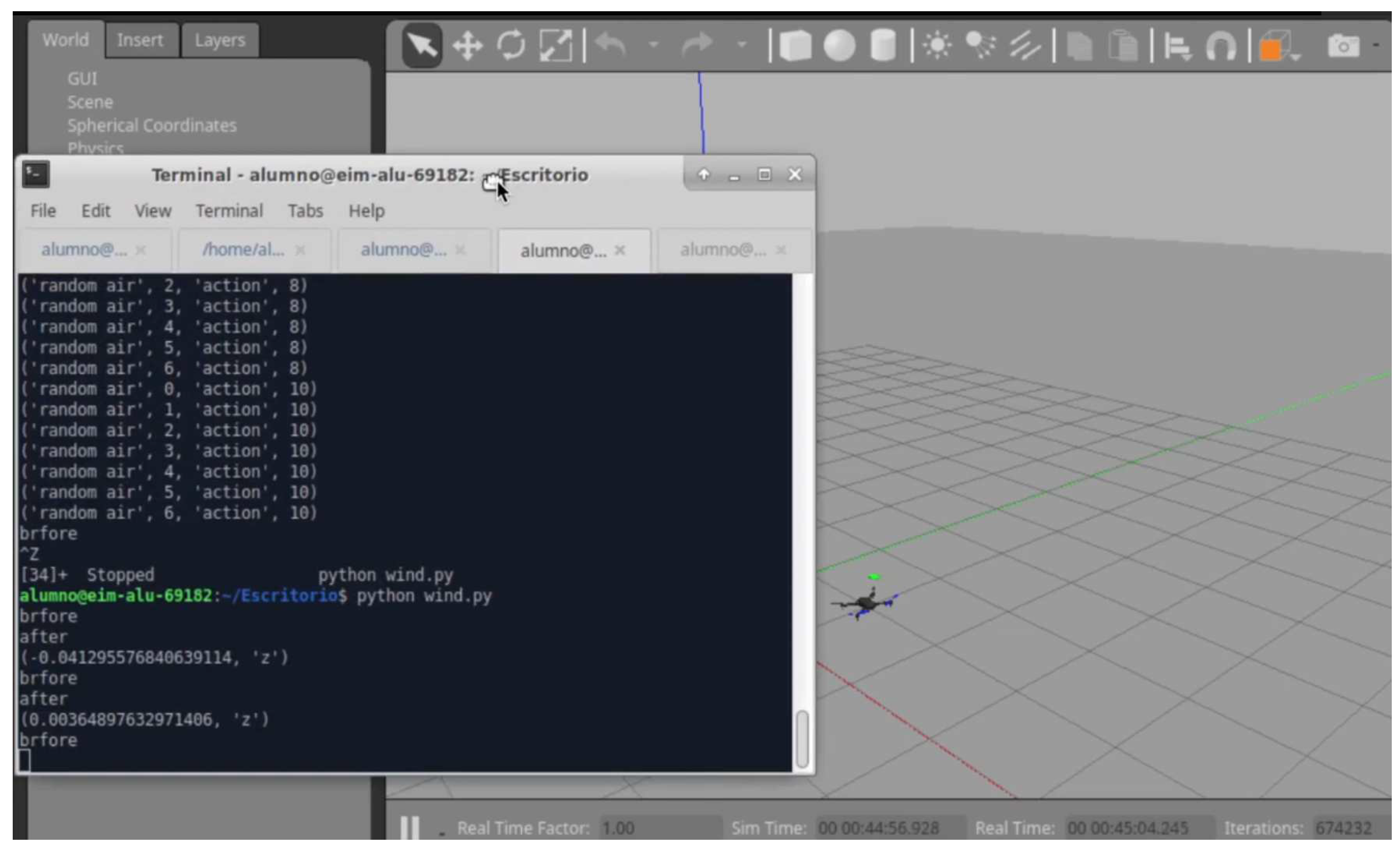
Initially, the quadcopter is loaded in the Gazebo environment in its initial state. A random wind is then generated and the disturbance is applied to the agent. The controller would then perform an action sending the signal to its motors, which would put it in a new state and receive a positive or negative reward based on its reward system. A diagram of this setup is shown in
Figure 1. A screenshot of the simulation environment can also be found in
Figure 2.
4.3. Agent
For this training, we used the PX4’s Iris optical flow model, a quadcopter with a lidar distance sensor for allowing correct measurement of the agent’s distance to the ground, along with other orientation sensors such as an IMU.
Our agent initially had 7 inputs, which referred to the states in the current timestep we wanted to observe: 3 axes for the drone position and rotation in its 4 quaternion components. Aside from that, we took these 7 inputs in the previous 3 timesteps so we network would be able to determine both the acceleration and direction of the agent, making a total of 28 inputs.
For the output, as mentioned above, the drone was able to perform 8 actions, which included going up, down, yaw , pitch , and roll .
4.4. Deep Q-Network
By using a traditional Q-learning algorithm, a table would have to be generated with each of the
q values for each of the actions, and exploring all these possible states would generate oversized value tables, with unrealistic consumption of time and resources. The algorithm is explained by Equation
7:
where
represents the Q-value or the action-value function, which is a mathematical function that estimates the expected total reward when taking action
a in state
s. In reinforcement learning, this function helps determine the quality of different actions in different states.
denotes the expected value operator under policy
. In other words, it represents the expected value of a random variable when following a particular policy
. In the context of Q-learning, it signifies taking the expected value over future rewards while following a policy.
The part specifies the conditional expectation. It calculates the expected sum of rewards given that, at time step t, the environment is in state and the agent takes action . In reinforcement learning, typically represents the cumulative rewards obtained from time step t onwards.
So, the equation as a whole represents the expected cumulative future rewards when starting in state s, taking action a, and following policy to make decisions. It’s a fundamental concept in reinforcement learning used for action selection and policy improvement.
That’s why we opted for the DQN algorithm in our training, as we needed the capacity to deal with a large number of states that would shape the continuous space we were training in. For that purpose, DQN is made up of two elements, a Q-Learning algorithm in the traditional sense and the inclusion of a convolutional network. The objective of the DQN algorithm was to optimize the optimal action-value function.
The DQN (Deep Q-Network) equation is an adaptation of the Bellman equation:
In the DQN (Deep Q-Network) adaptation, we use a deep neural network to estimate for all possible actions in the current state s. The network takes s as input and produces for all actions a. The agent selects the action with the highest for exploration/exploitation, and then observes the immediate reward and the next state . We use experience replay to store and sample batches of past transitions to train the neural network. The network is trained to minimize the difference between the current Q-value estimate and a target estimate based on the Bellman equation. This training process iterates over time to improve Q-value estimations and allows the agent to make optimal decisions in complex reinforcement learning environments.
This algorithm works in three steps:
The Q-table is generated (table where each action has an associated q value) from a Traditional Q-learning algorithm by a neural network. For that, it makes use of two neural networks, the policy/main network and the target network.
The best optimal action is chosen using the epsilon greedy strategy.
The weights of the model are adjusted according to the Bellman equation [
21].
4.5. External Disturbance Implementation
For the implementation of external disturbances, we directly apply the disturbance to the aircraft, necessitating the creation of a conversion rate from an external force to the drag it would generate in the aircraft. This required taking into account: the air density, approximately
kg·m
at Normal Temperature and Pressure (NTP) conditions; the drag coefficient, approximated by
; and the motor distance to its Center of Gravity (CG), approximately
m. The drag coefficient was assumed to be constant and equal in all three axes to account for the quadcopter symmetry in a worst-case scenario. In reality, the coefficient of drag is typically lower for a quadrotor UAV [
22]. This results in an actual aircraft capable of supporting even larger wind disturbance speeds.
The disturbance behavior was then emulated and the unpredictable acceleration was applied to the UAVs as follows:
The disturbance was generated parallel to the ground in a random direction and speed.
It then accelerated from 0 to max speed (up to 24 mph) at half of its lifetime and decelerated after that
This force would persist for 0 to 5 seconds and then subside for another 0-5 seconds range.
Finally, a new disturbance was generated, determined by a random variance with the previous one’s direction.
4.6. Training
Once we have defined the environment, the agent, the actions, and the implementation of external perturbations, it is time to carry out the training. The drone training was set to 1000 episodes and some supervision was made in the initial episodes to check any terminal states or incidents. The agent had the goal to reach a certain height of 6 meters while maintaining its position and stability to the maximum possible. After some tuning, the hyperparameters that gave the best results for the training are referenced in
Table 1.
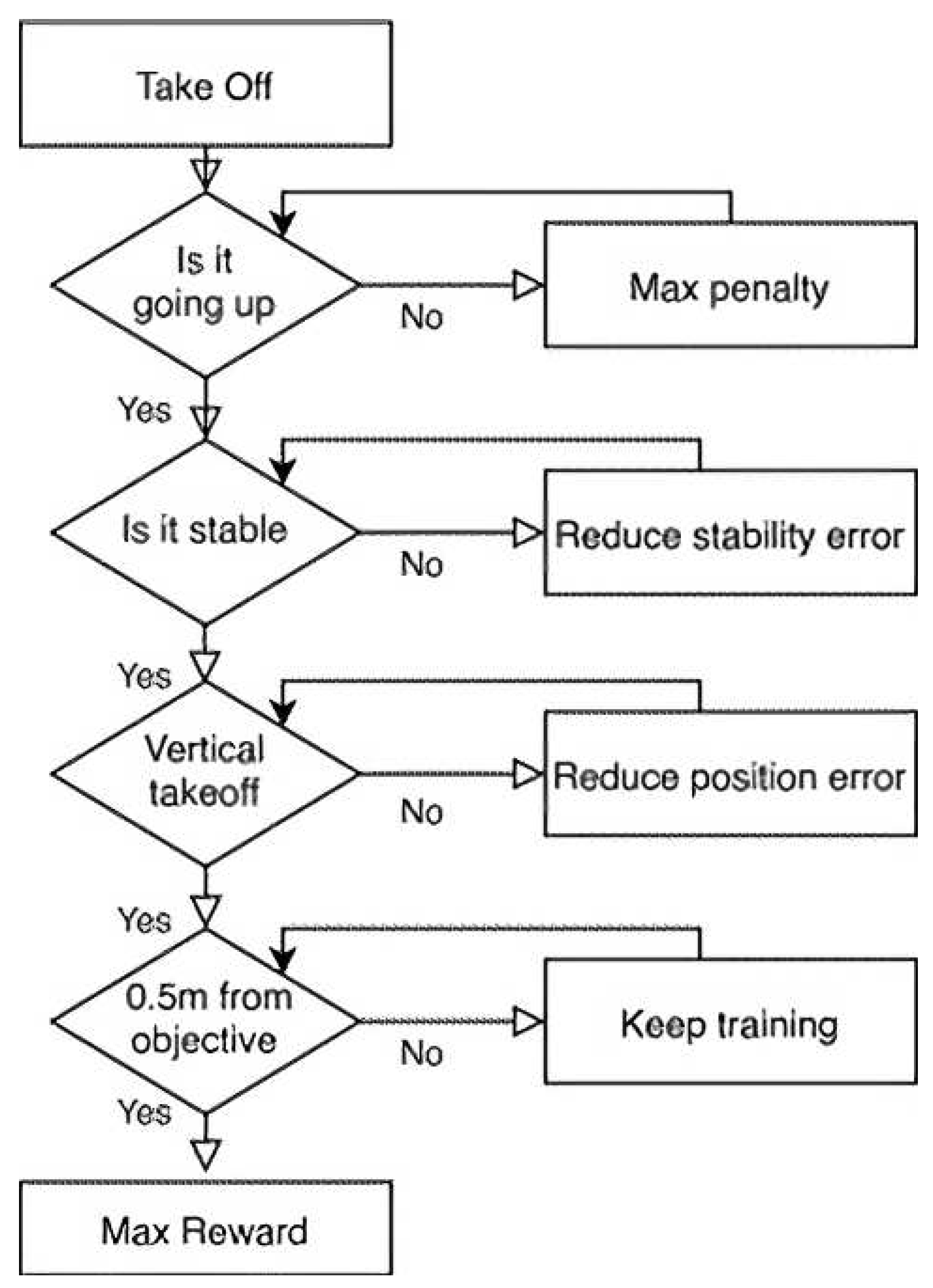
The flowchart shown in
Figure 3 describes how the rewards were sorted in terms of importance, being stability crucial in achieving the experiment, as taking off and reaching the goal with an unstable orientation was not desirable. The agent was rewarded for being stable and close to the vertical position and for getting closer to the end position. An additional maximum reward was included when the drone would stay within a range of 0.5 m of the goal. On the other side, the agent was punished for consecutive orientation error increases and for getting further from the vertical elevation guideline. For reference, some of the rewards are included in
Table 2.
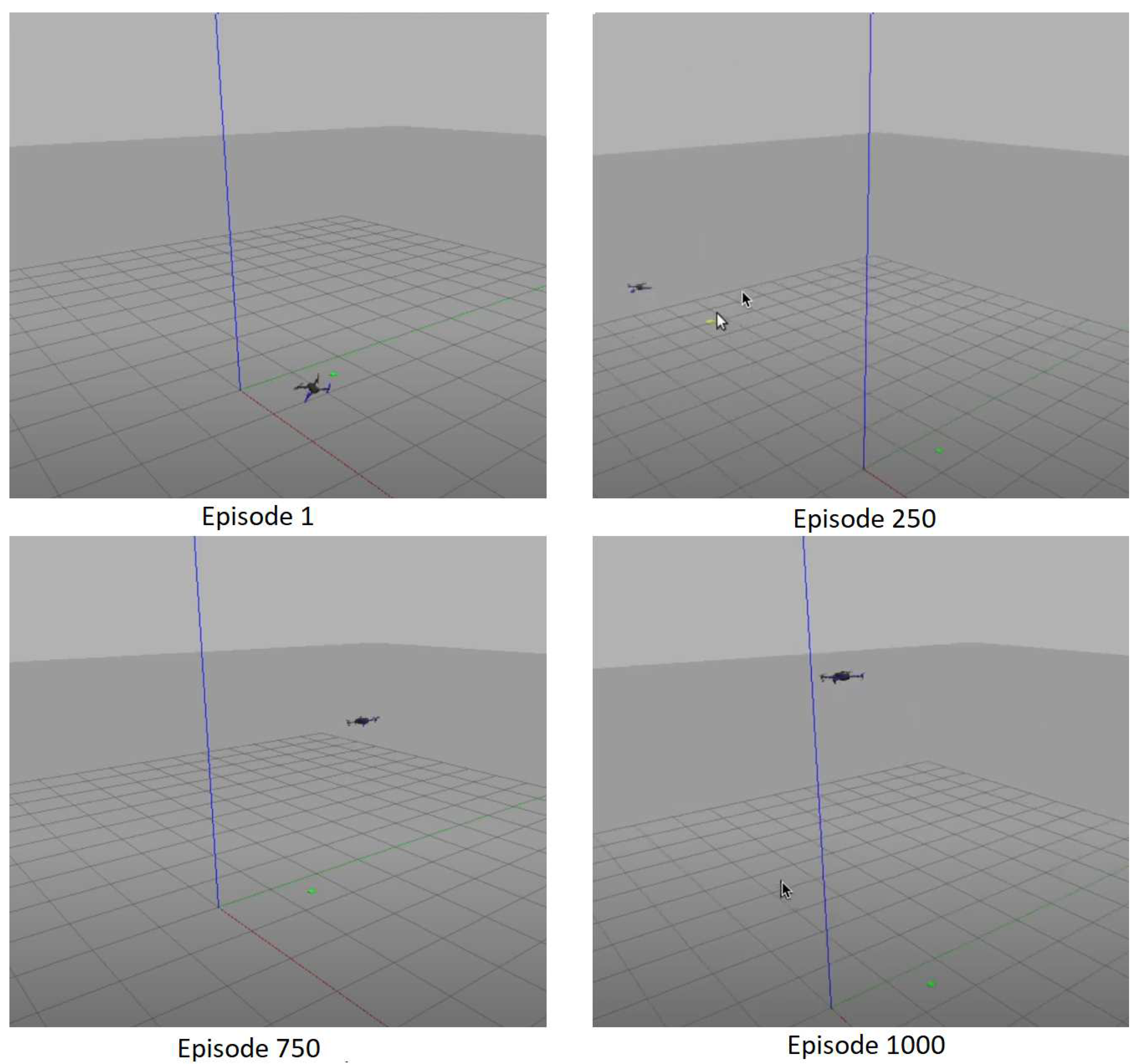
In
Figure 4, we can observe the evolution of the neural controller’s training over 1000 episodes. Initially, during the first 1000 episodes, the agent struggled to achieve takeoff because it needed to explore various actions. Consequently, it often encountered difficulties, such as being dragged by strong winds and experiencing crashes, as it had not yet capitalized on the position and orientation rewards and errors, as illustrated in Episode 250.
As exploration decreased and exploitation actions increased, the drone became more attuned to its environment. This allowed it to attain significant heights, even though it remained distant from the ultimate goal, as evidenced in Episode 750.
After fine-tuning the reward system, the drone ultimately converged around Episode 1000, successfully reaching its objective while maintaining minimal errors in both attitude and position metrics.
4.7. Reward Function
Some tuning on the reward function was required, as the agent learned to maximize its reward by not following the expected behavior and not taking off, as the reward for being stable in the ground was bigger than being unstable while going up, leading to a Cobra Effect Situation [
23]. To fix this, we included a maximum penalty to the agent for not moving at all, forcing it to go up.
Also, the reward for going up was not perfectly tuned, so the agent would take off as fast as possible and wouldn’t stop at the destination, as it was getting rewarded for reaching a higher position and therefore the drone would keep going up due to its inertial speed. Therefore, we added a reward for the motor’s output, so it would be rewarded for slowly decreasing its speed while getting closer to the objective height of 6 meters.
5. Results and discussion
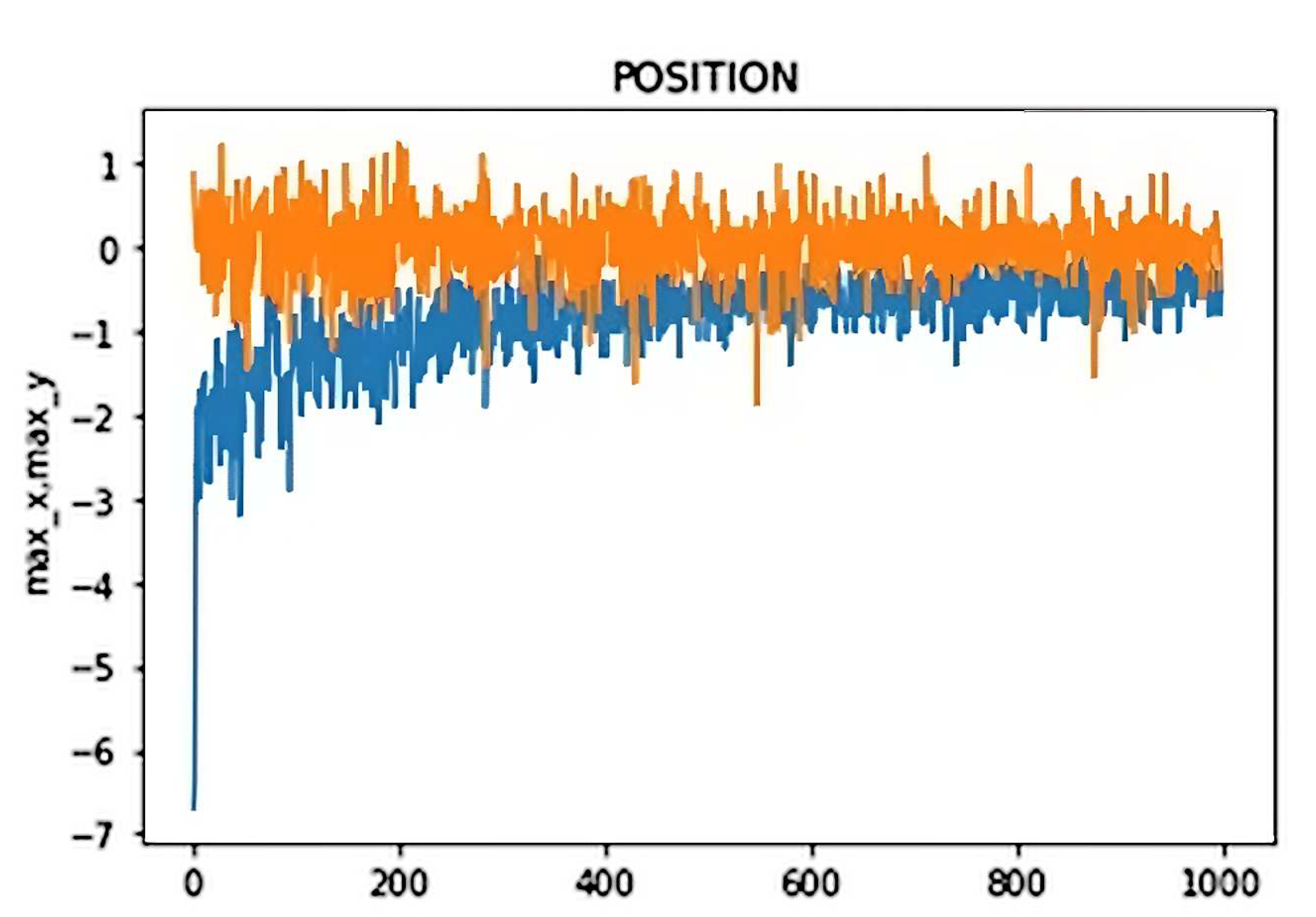
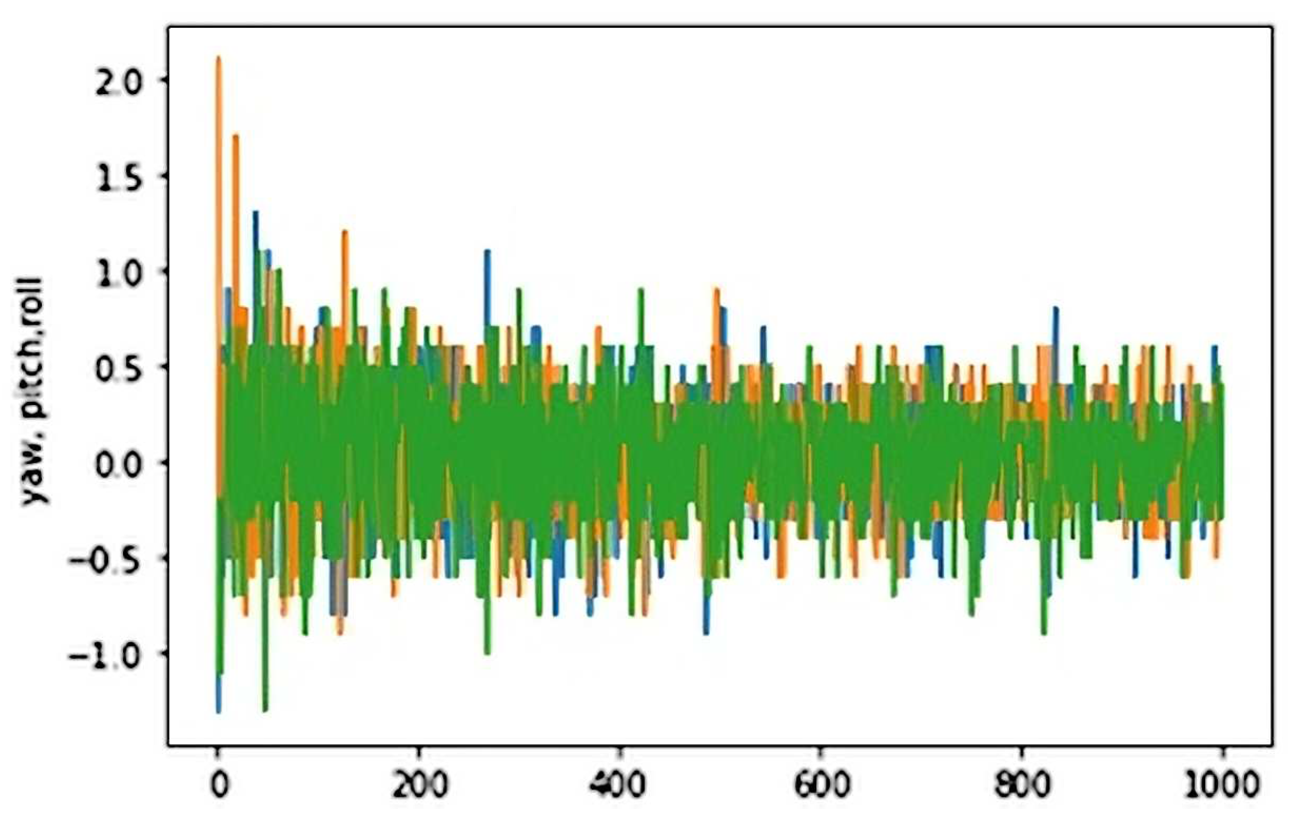
In this section, we will discuss the training results and demonstrate the effectiveness of the algorithm for take-off in windy conditions. The attitude and position errors were selected as the performance metrics. We measured attitude and position errors at the end of each training episode to evaluate the performance of the algorithm. The results have been compiled in
Figure 5 and Figure 7.
5.1. Attitude Error
If we focus on the attitude error first, it can be observed how the yaw, pitch, and roll errors (represented by orange, blue, and green lines, respectively) were significantly reduced while it was suffering from similar strength external force disturbances during the training. Values went from peaks of 2 rad (114 degrees) to values around 0.5 rad (28 degrees) in worst-case scenarios.
The first episodes proved to be hard for the agent, as external forces hit with the same strength all over the training and were flipping the drone upside down, having to reset the episode in several cases.
5.2. Location/Position Error
As shown in
Figure 7, the drone deviation due to these external forces pushing in both
x and
y horizontal axes was reduced from 7 meters to a maximum detour of 1 m while it was performing the vertical ascension. It showed a big improvement over the first 200 episodes where it was constantly taken out of the training area by the external disturbance (3 meters), and slowly started learning to recover its position after being pushed away, and finally facing this force so it could compensate the negative drag of it.
Figure 6.
Position error in 1000 episodes
Figure 6.
Position error in 1000 episodes
5.3. Actions Required
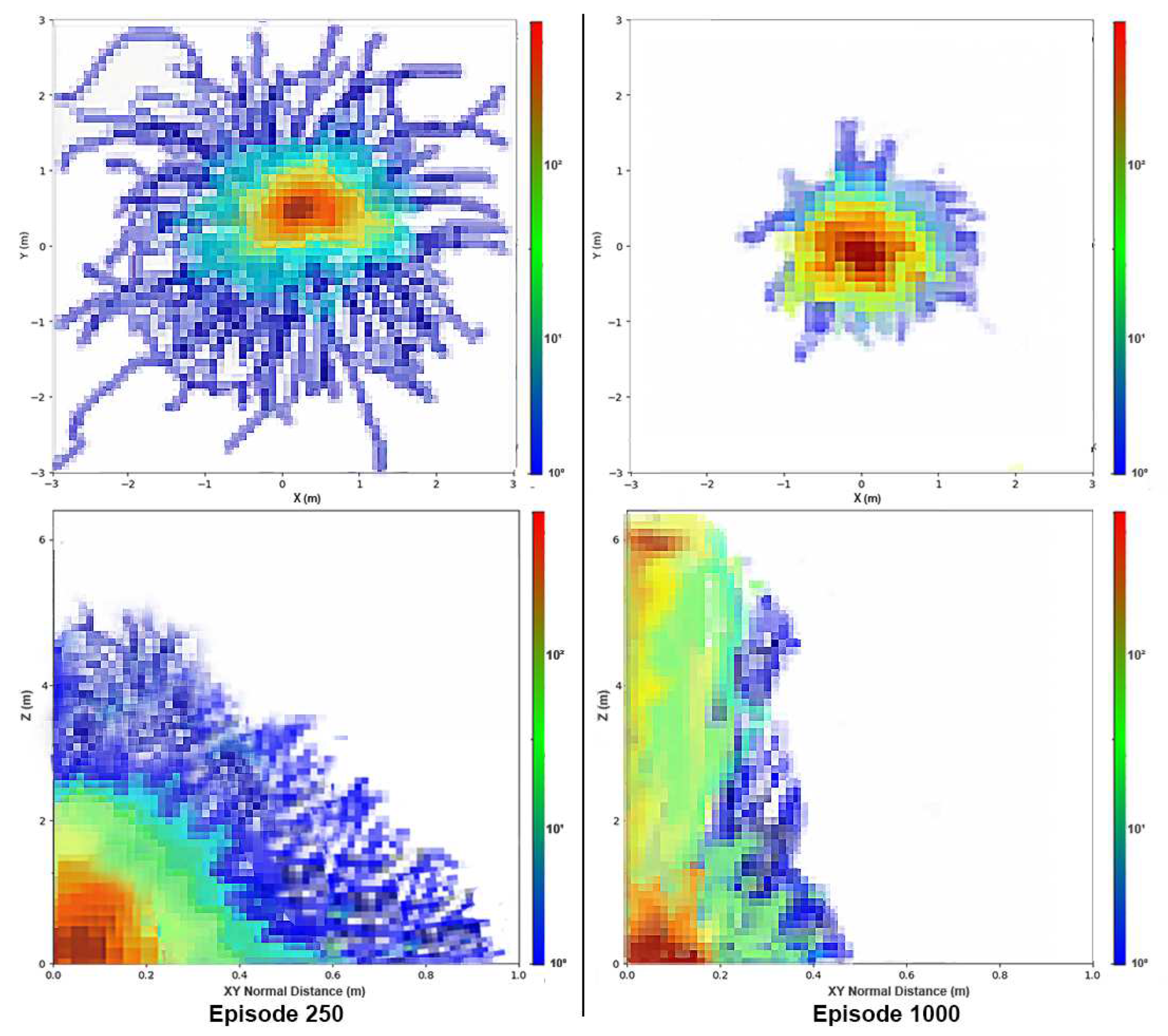
Finally, the agent learned to perform the lift from the ground by using fewer and fewer actions each time.
Figure 7 represents the number of steps it took the drone to reach the elevated target at 6 meters. The captured data is for the last training. This means it belongs to the first time the agent is able to converge and solve the problem. In this graph, blue represents total actions, which is the sum of both exploration (orange) and exploitation actions(green). It can be seen how due to the Epsilon greedy policy, the number of exploration steps was reduced as long as it learned to converge and did not need any exploration to understand the environment. It started by using around 200 actions to perform the elevation and was able to reduce the needed actions to around 50 by the end of training in episode 1000. Thus, we have demonstrated that the algorithm is capable of developing successful take-offs with a smaller number of actions even in adverse wind conditions.
Figure 7.
DQN for takeoff maneuver in the last training. The upper images show the zenithal heatmap, while the bottom images show the lateral one
Figure 7.
DQN for takeoff maneuver in the last training. The upper images show the zenithal heatmap, while the bottom images show the lateral one
6. Conclusion
In this paper, we proposed a reinforcement learning method for taking off with a drone under wind conditions that are not suitable for human piloting, with wind disturbances of up to 24 mph. The proposed system utilized the DQN algorithm to train the agent to achieve vertical elevation within a simulator. After 1000 episodes, the agent demonstrated its capability to maintain stability under these challenging conditions. In future research, we plan to explore individual motor control, implement it on hardware to test its performance against real-world forces and compare its capacity and responsiveness with that of a trained human pilot.
Author Contributions
X.O.: Methodology, conceptualization, formal analysis, investigation, writing, software, validation, visualization, original draft preparation. D.A.: Conceptualization, methodology, formal analysis. P.P.: Investigation, data curation, review. M.P.: review, resources, editing, supervision. J.V.: review, resources, supervision, project administration, funding acquisition.
Funding
This work has been supported in part by the Ministerio de Ciencia e Innovación (Spain) and European Union NextGenerationEU, Spain under the research grant TED2021-131716B-C21 SARA (Data processing by superresolution algorithms); in part by Agencia Estatal de Investigación (AEI), Spain and European Union NextGenerationEU/PRTR, Spain PLEC2021-007997: Holistic power lines predictive maintenance system and CONDOR-Connected PID2021-127409OB-C31.
Institutional Review Board Statement
Not applicable.
Informed Consent Statement
Not applicable.
Data Availability Statement
Not applicable.
Conflicts of Interest
The authors declare no conflict of interest. The funders had no role in the design of the study; in the collection, analyses, or interpretation of data; in the writing of the manuscript; or in the decision to publish the results.
References
- Sutton, R.S.; Barto, A.G. Reinforcement learning: An introduction; MIT press, 2018.
- Mnih, V.; Kavukcuoglu, K.; Silver, D.; Rusu, A.A.; Veness, J.; Bellemare, M.G.; Graves, A.; Riedmiller, M.; Fidjeland, A.K.; Ostrovski, G.; others. Human-level control through deep reinforcement learning. nature 2015, 518, 529–533. [Google Scholar] [CrossRef] [PubMed]
- Koenig, N.; Howard, A. Design and use paradigms for gazebo, an open-source multi-robot simulator. 2004 IEEE/RSJ international conference on intelligent robots and systems (IROS)(IEEE Cat. No. 04CH37566). IEEE 2004, 3, 2149–2154. [Google Scholar]
- Matignon, L.; Laurent, G.J.; Le Fort-Piat, N. Reward function and initial values: Better choices for accelerated goal-directed reinforcement learning. International Conference on Artificial Neural Networks. Springer, 2006, pp. 840–849.
- Simon, N.; Piqué, A.; Snyder, D.; Ikuma, K.; Majumdar, A.; Hultmark, M. Fast-response hot-wire flow sensors for wind and gust estimation on UAVs. Measurement Science and Technology 2022, 34, 025109. [Google Scholar] [CrossRef]
- Har-Peled, S.; Indyk, P.; Motwani, R. Approximate nearest neighbor: Towards removing the curse of dimensionality 2012.
- Zheng, X.; Yu, X.; Yang, X.; Zheng, W.X. Adaptive NN Zeta-Backstepping Control With Its Application to a Quadrotor Hover. IEEE Transactions on Circuits and Systems II: Express Briefs 2023, pp. 1–1. [CrossRef]
- Liu, K.; Yang, P.; Wang, R.; Jiao, L.; Li, T.; Zhang, J. Observer-Based Adaptive Fuzzy Finite-Time Attitude Control for Quadrotor UAVs. IEEE Transactions on Aerospace and Electronic Systems 2023, pp. 1–17. [CrossRef]
- Kumar, S.; Dewan, L. Hybrid Controller for Soft Landing of a Quadcopter. IETE Journal of Research 2023, 0, 1–14. [Google Scholar] [CrossRef]
- Wang, J.; Zhu, B.; Zheng, Z. Robust Adaptive Control for a Quadrotor UAV With Uncertain Aerodynamic Parameters. IEEE Transactions on Aerospace and Electronic Systems 2023, 1–15. [Google Scholar] [CrossRef]
- Koch III, W.F. Flight controller synthesis via deep reinforcement learning. PhD thesis, Boston University, 2019.
- Schulman, J.; Wolski, F.; Dhariwal, P.; Radford, A.; Klimov, O. Proximal policy optimization algorithms. arXiv 2017, arXiv:1707.06347 2017. [Google Scholar]
- Che-Cheng, C.; Tsai, J.; Peng-Chen, L.; Lai, C.A. Accuracy Improvement of Autonomous Straight Take-off, Flying Forward, and Landing of a Drone with Deep Reinforcement Learning. International Journal of Computational Intelligence Systems 2020, 13, 914. [Google Scholar] [CrossRef]
- Cetin, E.; Barrado, C.; Muñoz, G.; Macias, M.; Pastor, E. Drone navigation and avoidance of obstacles through deep reinforcement learning. 2019 IEEE/AIAA 38th Digital Avionics Systems Conference (DASC). IEEE. 2019, 1–7. [Google Scholar]
- Shah, S.; Dey, D.; Lovett, C.; Kapoor, A. Airsim: High-fidelity visual and physical simulation for autonomous vehicles. Field and Service Robotics: Results of the 11th International Conference. Springer, 2018, pp. 621–635.
- Rodriguez-Ramos, A.; Sampedro, C.; Bavle, H.; De La Puente, P.; Campoy, P. A deep reinforcement learning strategy for UAV autonomous landing on a moving platform. Journal of Intelligent & Robotic Systems 2019, 93, 351–366. [Google Scholar]
- Luukkonen, T. Modelling and control of quadcopter. Independent research project in applied mathematics, Espoo 2011, 22. [Google Scholar]
- MASSÉ, C.; GOUGEON, O.; NGUYEN, D.T.; SAUSSIÉ, D. Modeling and Control of a Quadcopter Flying in a Wind Field: A Comparison Between LQR and Structured Control Techniques. 2018 International Conference on Unmanned Aircraft Systems (ICUAS), 2018, pp. 1408–1417. [CrossRef]
- Lamping, A.P.; Ouwerkerk, J.N.; Cohen, K. Multi-UAV control and supervision with ROS. 2018 aviation technology, integration, and operations conference, 2018, p. 4245.
- Meier, L.; Honegger, D.; Pollefeys, M. PX4: A node-based multithreaded open source robotics framework for deeply embedded platforms. 2015 IEEE international conference on robotics and automation (ICRA). IEEE, 2015, pp. 6235–6240.
- Bellman, R. A Markovian decision process. Journal of mathematics and mechanics 1957, 679–684. [Google Scholar] [CrossRef]
- Hattenberger, G.; Bronz, M.; Condomines, J.P. Evaluation of drag coefficient for a quadrotor model. International Journal of Micro Air Vehicles 2023, 15, 17568293221148378. [Google Scholar] [CrossRef]
- Warczak Jr, P. The cobra effect: Kisor, Roberts, and the law of unintended consequences. Akron L. Rev. 2020, 54, 111. [Google Scholar] [CrossRef]
|
Disclaimer/Publisher’s Note: The statements, opinions and data contained in all publications are solely those of the individual author(s) and contributor(s) and not of MDPI and/or the editor(s). MDPI and/or the editor(s) disclaim responsibility for any injury to people or property resulting from any ideas, methods, instructions or products referred to in the content. |
© 2023 by the authors. Licensee MDPI, Basel, Switzerland. This article is an open access article distributed under the terms and conditions of the Creative Commons Attribution (CC BY) license (http://creativecommons.org/licenses/by/4.0/).
