1. Introduction
Many practical problems of the modern world can be thought of either as data fitting problems, as for example, problem from physics [
1,
2], chemistry [
3,
4], economics [
5,
6], medicine [
7,
8], etc. A machine learning tool, commonly used to handle these problems, is the Radial Basis Function (RBF) artificial neural network [
9,
10]. Usually, an RBF network is expressed using the following equation:
where the symbols in the equation are defined as follows:
The vector is the input pattern from the objective problem. For the rest of this paper the notation d will be used to represent the number of elements in .
The parameter k denotes the number of weights used to train the RBF network and the associated vector of weights is denotes as .
The vectors stand for the so - called centers.
The outcome of the equations stands for the estimated value of the network for the input pattern .
The function
usually is a Gaussian function given by:
The RBF networks were used in many cases, such as problems from physics [
11,
12,
13,
14], solving differential equations [
15,
16,
17], robotics [
18,
19], face recognition [
20], digital communications [
21,
22], chemistry problems [
23,
24], economic problems [
25,
26,
27], network security problems [
28,
29] etc. Also, recently a variety of papers have appeared proposing novel initialization techniques for the network parameters [
30,
31,
32]. Also, Benoudjit et al [
33] discuss the effect of kernel widths on RBF networks. Moreover, Neruda et al [
34] presents a comparison of some learning methods for RBF networks. Additionally, a variety of pruning techniques [
35,
36,
37] have been proposed to reduce the number of required parameters of the RBF networks. Due to the widespread usage of RBF networks but also because considerable computing time is often required for their effective training, in recent years a series of techniques have been proposed [
38,
39] for the exploitation of parallel computing units to adjust the parameters of neural networks.
The current work proposes a two phase method for the effective adjustment of the parameters of RBF networks in order to minimize the so -called training error given by:
Where the parameter
m denotes the number of input patterns, the
values represent the expected output for the input pattern
. The vector
g represents the parameter set of the RBF network. During the first phase, an attempt is made to bound the parameter values to intervals in which the training error of equation
3 is likely to be significantly reduced. The identification of the most promising intervals for the parameters is performed using a technique that utilizes Grammatical Evolution[
40]. First, an estimate of an interval of values for the network parameters is made using the Kmeans algorithm [
41]. Then, with the help of Grammatical Evolution, a series of division rules are applied to the initial interval of values in order to find a range of values that significantly reduces the training error. During the second phase, the parameters of the RBF network can be trained within the optimal range found in the first phase using some global optimization method [
42,
43]. In the proposed approach, the widely used method of genetic algorithm [
44,
45,
46] was used for the second phase of the process.
The rest of this paper is divided in the following sections: in
Section 2 the proposed method is fully described, in
Section 3 the datasets used in the experiments are listed as well as the experimental results and finally in
Section 4 some conclusions are provided.
2. Method description
This section begins with a detailed description of the Grammatical Evolution technique and the grammar that will be used to generate partition rules for the parameter set of RBFs. Subsequently, the first phase of the proposed methodology will be extensively analyzed and then the second phase, where a Genetic Algorithm will be applied to the outcome of the first phase.
2.1. Grammatical Evolution
Grammatical evolution is a genetic algorithm where the chromosomes stand for the production rules of any given BNF (Backus–Naur form) grammar[
47]. Grammatical Evolution has been used successfully in a variety of cases, such as function approximation[
48,
49], solution of trigonometric equations [
50], automatic music composition of music [
51], neural network construction [
52,
53], creating numeric constraints[
54]
,video games [
55,
56], estimation of energy demand[
57], combinatorial optimization [
58], cryptography [
59] etc. The BNF grammar can be used to describe the syntax of programming languages and usually it is defined as the set
where
N is the set of the so - called non-terminal symbols. Every non - terminal symbol is associated with a series of production rules used to produce terminal symbols.
T is the set of terminal symbols.
S is a the start symbol of the grammar and .
P is a set of production rules, used to produce terminal symbols from non - terminal symbols. These rules are in the form or.
The algorithm starts from the symbol S and gradually creates terminal symbols by replacing non-terminal symbols with the right hand of the selected production rule. The rule is selected through the following procedure:
Read the next element V from the current chromosome.
The production rule is selected as: Rule = V mod R, where R is the total number of production rules for the current non – terminal symbol.
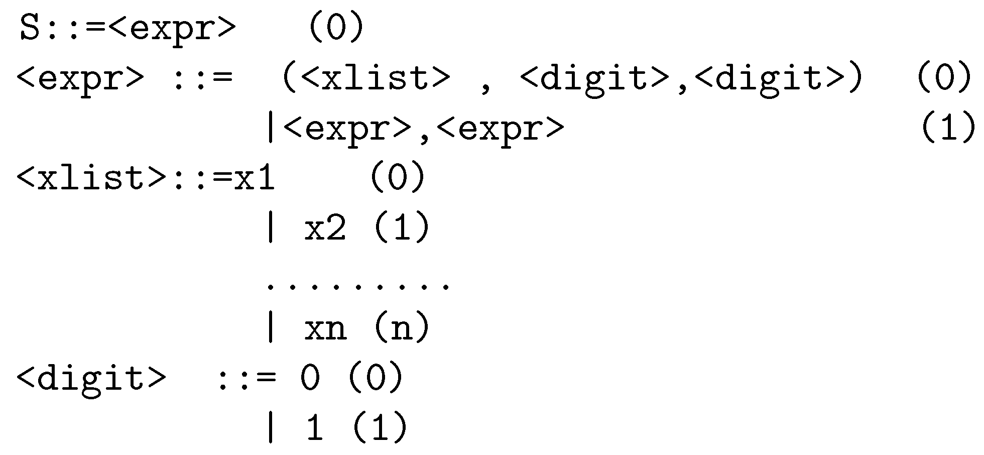
The BNF grammar used in this work is presented in
Figure 1. The symbols enclosed in <> denote the non-terminal symbols of the grammar. The numbers in parentheses in the right part of the grammar indicate production rule sequence numbers. The number n is the total number of parameters of the problem. In the case of this paper it is the total number of parameters of the RBF network. For the current work, the number
n can be computed using the following formula:
The number n is computed as follows:
For every center there are d variables. Hence, the total number of parameters required by the centers are .
Every Gaussian unit required an additional parameter , which means k more parameters.
The weight vector used in the output has k parameters.
As an example of production considered the chromosome
and
. The steps to produce the final program
are outlined in
Table 1. Every partition program consists of a series of partition rules. Each partition rule contains three elements:
The variable for which its original interval will be partitioned, for example .
An integer number with values 0 and 1 at the left end of the value interval. If this value is 1, then the left end of the corresponding variable’s value field will be divided by two, otherwise no change will be made.
An integer number with values 0 and 1 at the right end of the range of values of the variable. If this value is 1, then the right end of the corresponding variable’s value field will be divided by two, otherwise no change will be made.
Hence, for the example program the two partition rules will divide the right end of the variable and the left end of the variable .
2.2. The first phase of the proposed algorithm
The first step of the first phase of the proposed method is to initialize the bounds of the RBF network. For this initialization, the K-Means algorithm [
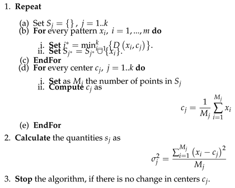
41] technique is used, which is also used for the traditional RBF network training technique. A description of this algorithm in a series of steps is shown in Algorithm 1.
|
Algorithm 1:The K-Means algorithm. |
 |
Having calculated the centers
and the corresponding variances
, the algorithm continues to compute the vectors
with dimension
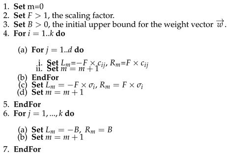
n, that will be used as the initial bounds of the parameters. The above vectors are calculated through the procedure of the Algorithm 2.
|
Algorithm 2:Algorithm to locate the vectors
|
 |
The bounds for the first variables of any given RBF network are considered as a multiple of the quantity F with the values calculated by the K-Means algorithm. The positive constant B is used to initialize the intervals for the weight . Afterwards, the following genetic algorithm is executed to locate the most promising vectors for the RBF parameters:
Set as the number of chromosomes for the Grammatical Evolution.
Set as k the number of weights of the RBF network.
Set the maximum number of allowed generations.
Set as the selection rate of the algorithm, with .
Set as the mutation rate, with .
Set as the number of randomly created RBF networks, used in the fitness calculation.
Initialize randomly the chromosomes as sets of random numbers.
Set , the fitness of the best chromosome. The fitness function of any given chromosome g is considered as an interval
Set iter=0.
-
For
do
- (a)
Create the partition program
using the grammar of
Figure 1 for the chromosome
.
- (b)
Produce the bounds for the partition program .
- (c)
Set
- (d)
-
For
do
Create randomly a set of parameters
Calculate the error
If
then
If
then
- (e)
EndFor
- (f)
Set the fitness
EndFor
-
Apply the selection procedure: Initially, the chromosomes of the population are sorted according to their fitness values. In order to compare two fitness values
and
the
operator is used:
Hence, the fitness value is considered smaller than if . The first chromosomes with smaller fitness values are transferred intact to the next generation. The remaining chromosomes are replaced by offspring created in the crossover procedure. During the selection process for each offspring, two parents are selected from the population using the tournament selection.
Apply the crossover procedure. The crossover procedure will create new
chromosomes. For each new offspring two parents are selected from the population using the tournament selection. For each pair
of selected parents, two new chromosomes
and
are produced using the one - point crossover, shown in
Figure 2.
Apply the mutation procedure. For each element of every chromosome, a random number is drawn. The corresponding element is altered randomly if .
Set iter=iter+1
If goto step 10.
2.3. The second phase of the proposed algorithm
The second phase utilizes a genetic algorithm, to optimize the parameters of the RBF network within the best interval returned by the first phase of the method. The layout of each chromosome is shown in
Figure 3.
-
Initialization Step
- (a)
Set as the number of chromosomes.
- (b)
Set the maximum number of allowed generations.
- (c)
Set k the weight number of the RBF network.
- (d)
Get the best interval
S from the first step of sub
Section 2.2.
- (e)
Initialize randomly the chromosomes in in S.
- (f)
Set as the selection rate of the algorithm, with .
- (g)
Set as the mutation rate, with .
- (h)
Set iter=0.
-
Fitness calculation Step
- (a)
-
For
do
- (b)
EndFor
-
Genetic operations step
- (a)
Selection procedure. The chromosomes are sorted according to their fitness values. The chromosomes with the lowest fitness values are transferred intact to the next generation. The remaining chromosomes are substituted by offspings created in the crossover procedure. During the selection process for each offspring, two parents are selected from the population using the tournament selection.
- (b)
-
Crossover procedure: For every pair
of selected parents two additional chromosomes
and
are produced using the following equations:
The value
is considered as a random number with the property
[
60].
- (c)
Mutation procedure: For each element of every chromosome, a random number
is drawn. The corresponding element is altered randomly if
.
-
Termination Check Step
- (a)
Set
- (b)
If goto step 2.
3. Experiments
The suggested method was tested on a series of classification and regression problems from the relevant literature and was compared against some other well -known machine learning models. The following databases were used to obtain the datasets:
3.1. Experimental datasets
The classification datasets have as follows:
Appendictis dataset, a medical dataset proposed in [
62].
Australian dataset [
63], an dataset related to economic data.
Balance dataset [
64], which used to predict psychological states.
Cleveland dataset, which is a medical dataset related to heart diseases [
65,
66].
Dermatology dataset [
67], a medical dataset.
Heart dataset [
69], a medical dataset related to heart diseases.
HouseVotes dataset [
70], related to Congressional voting records.
Ionosphere dataset, used for classification of radar returns from the ionosphere [
71,
72].
Liverdisorder dataset [
73], a medical dataset.
Mammographic dataset [
74], used to identify breast tumors.
Parkinsons dataset, a medical dataset related to the Parkinson’s Disease[
75].
Pima dataset, a medical dataset[
76].
Popfailures dataset [
77], a dataset related to climate measurements.
Spiral dataset, an artificial dataset with 2 features and two classes. The patterns for the first class are produced according to the equation: and the second class data using:
Saheart dataset [
79], a medical dataset about heart diseases.
Segment dataset [
80], an image processing dataset.
Wdbc dataset [
81], used to identify breast tumors.
Wine dataset, used to classify wines [
82,
83].
Eeg dataset, a medical dataset about EEG measurements[
84] . The datasets used are denoted as Z_F_S, ZONF_S and ZO_NF_S.
Zoo dataset [
85], used to classify animals.
The following regression datasets were used in the experiments:
Airfoildataset, a dataset derived from NASA [
87].
Baseball dataset, a dataset used in baseball games.
BK dataset [
88], used to predict the points in a basketball game.
BL dataset, an electrical engineering dataset.
Concrete dataset, related to civil engineering[
89].
Dee dataset, used to predict the energy consumption.
Diabetes dataset, a medical dataset.
FA dataset, related to fat measurements.
Housing dataset, provided in [
90].
MORTGAGE dataset, which contains economic data.
Quake dataset, used to predict earthquakes [
94].
Treasure dataset, which contains data about the economy.
Wankara dataset, a dataset used for climate measurements.
3.2. Experimental results
The used RBF network was coded in ANSI C++ using the freely available Armadillo library [
95]. The optimization methods used were also freely available from the OPTIMUS computing environment, downloaded from
https://github.com/itsoulos/OPTIMUS/(accessed on 9 September 2023). To validate the results, the 10 - fold validation technique was used in all datasets. The experiments were conducted 30 times for every dataset using a different seed for the random generator each time. In the conducted experiments, the drand48() random function of the C - programming language was employed. The average classification error is reported for the case of classification datasets and the average mean test error for the regression datasets. The machine used in the experiments was an AMD Ryzen 5950X with 128GB of RAM, running the Debian Linux operating system. All the values for the parameters of the used algorithms are shown in
Table 2. The results obtained for the classification datasets are shown in
Table 3 and for the regression datasets are listed in
Table 4.
The following applies to the results tables:
The column NN-PROP represents an artificial neural network [
96,
97] with 10 hidden nodes trained with the Rprop method [
98].
The column RBF-KMEANS represents the original two -phase training method for RBF networks, where in the first phase the centers and variances are estimated through the K-Means algorithm and in the second phase the output weights are calculated by solving a linear system of equations.
The column GENRBF stands for the RBF training method introduced in [
99].
The column PROPOSED represents the results obtained by the proposed method.
An extra line was also added to the experimental tables under the title AVERAGE. This line represents the average classification or regression error for all datasets.
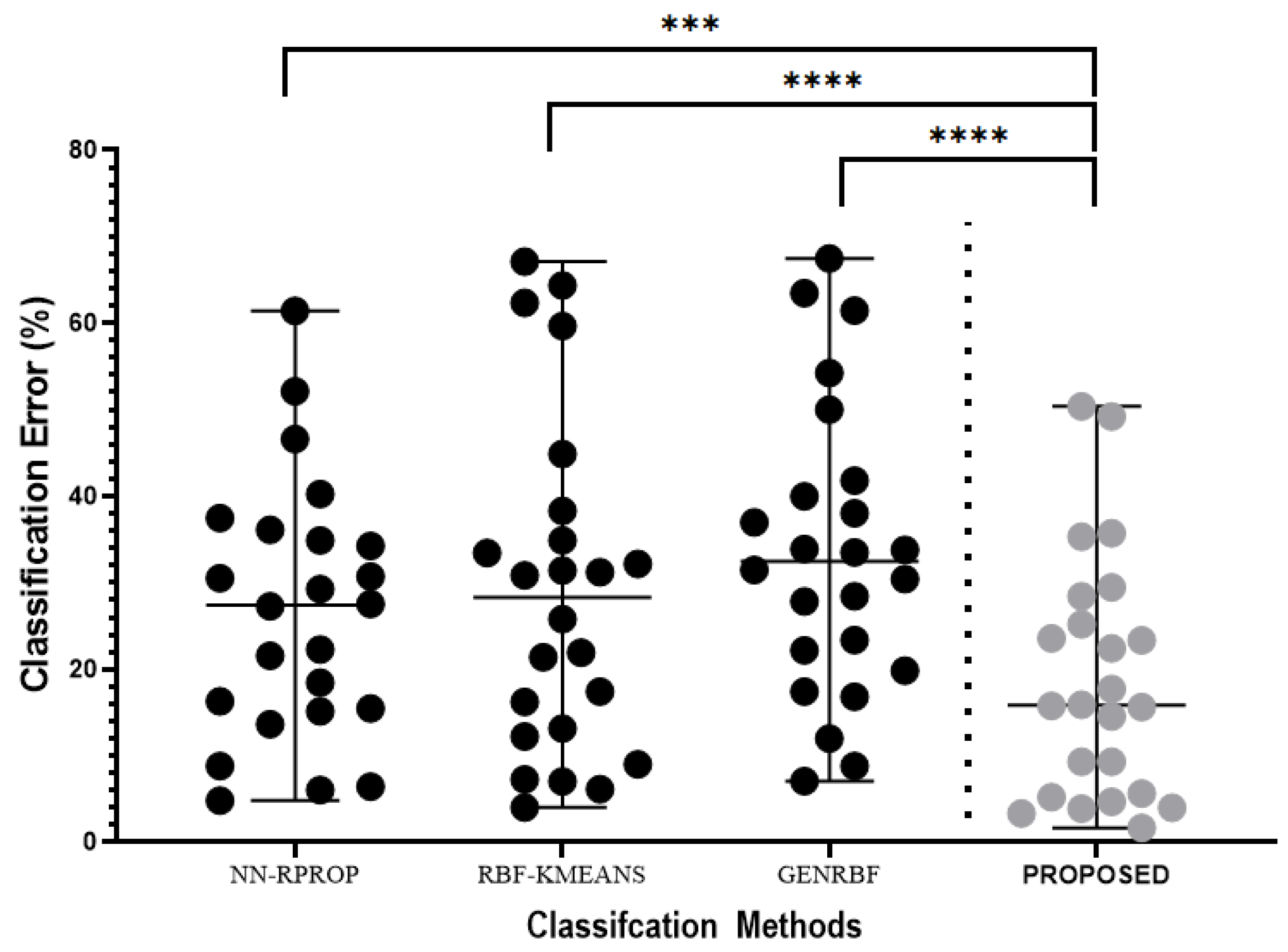
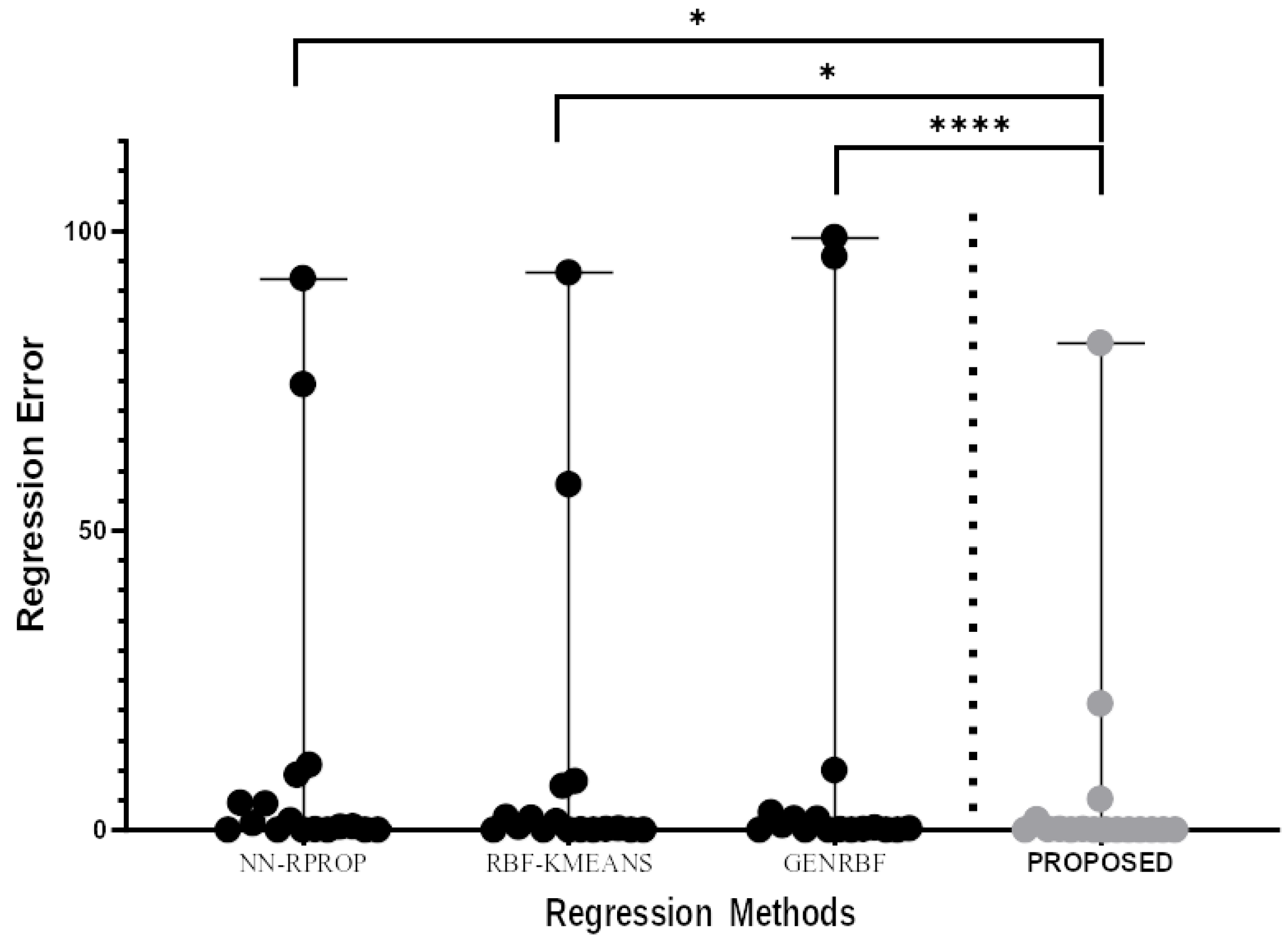
On average, the proposed technique appears to be 30-40% more accurate than the immediate best. In many cases, this percentage exceeds 70%. Moreover, in the vast majority of problems, the proposed technique significantly outperforms the next best available method in terms of test error. However, the proposed technique consists of two stages and in each of them a genetic algorithm should be executed. This means that it is significantly slower in computing time compared to the rest of the techniques and, of course, it needs more computing resources. Of course, since we are talking about Genetic Algorithms, the training time required could be significantly reduced by using parallel techniques that take advantage of modern parallel computing structures such as the MPI interface [
100] or the OpenMP library [
101]. The superiority of the proposed technique is also reinforced by the statistical tests carried out on the experimental results and presented in
Figure 4 and
Figure 5.
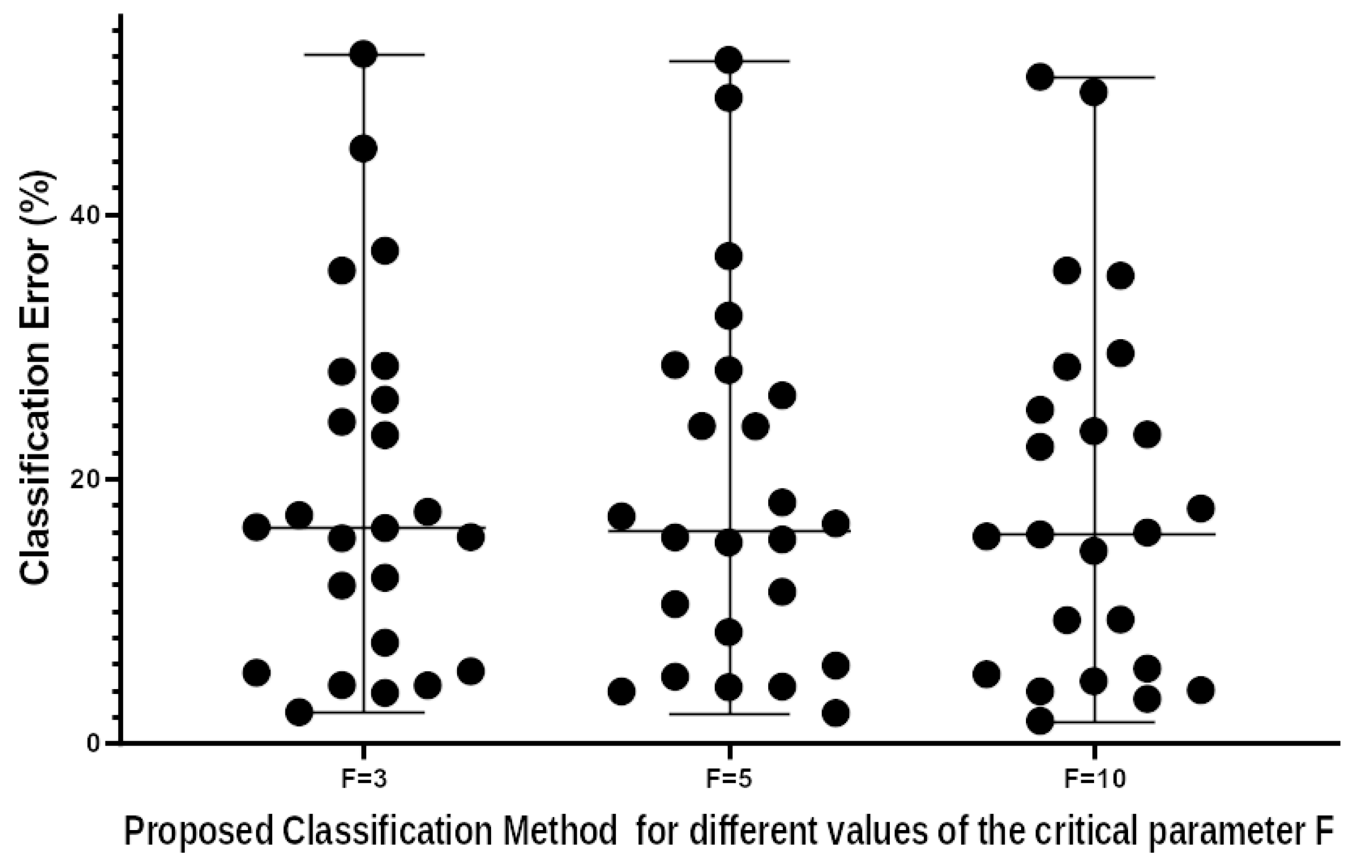
In addition, an additional set of experiments was performed on the classification data in which the critical parameter
F took the values 3, 5 and 10. The aim of this set of experiments was to establish the sensitivity of the proposed technique to changes in its parameters. The experimental results are presented in the
Table 5 and a statistical test on the results is presented in
Figure 6. The results and the statistics test indicate that there is no significant difference in the efficiency of the method for different values of the critical parameter
F.
4. Conclusions
A two-step method was presented in the present work to train RBF neural networks. In the first stage of the application, using Grammatical Evolution, the field of values of the neural network parameters is partitioned, so as to find a promising range that may contain low values of the training error. In the second stage, the neural network parameters are trained within the best range of values found in the first stage. The training of the parameters of the second phase is carried out using a Genetic Algorithm. The proposed method was applied on a wide series of well -known datasets from the relevant literature and was tested against a series of machine learning models. From the comparison of the results and their statistical processing, it was clearly seen that the proposed technique outperforms the others with which the comparison was made, both in classification datasets and regression datasets. Future improvements to the proposed method may include:
Application of the proposed method to other types of artificial neural networks.
Implementation of crossover and mutation techniques that focus more on the existing interval construction technique for the model parameters.
Incorporation of parallel programming techniques to speed up the method.
Author Contributions
I.G.T., A.T. and E.K. conceived the idea and methodology and supervised the technical part regarding the software. I.G.T. conducted the experiments, employing several datasets, and provided the comparative experiments. A.T. performed the statistical analysis. E.K. and all other authors prepared the manuscript. E.K. and I.G.T. organized the research team and A.T. supervised the project. All authors have read and agreed to the published version of the manuscript.
Funding
This research received no external funding.
Institutional Review Board Statement
Not applicable.
Informed Consent Statement
Not applicable.
Institutional Review Board Statement
Not applicable.
Acknowledgments
The experiments of this research work were performed at the high performance computing system established at Knowledge and Intelligent Computing Laboratory, Department of Informatics and Telecommunications, University of Ioannina, acquired with the project “Educational Laboratory equipment of TEI of Epirus” with MIS 5007094 funded by the Operational Programme “Epirus” 2014–2020, by ERDF and national funds.
Conflicts of Interest
The authors declare no conflict of interest.
Sample Availability
Not applicable.
References
- Mjahed, M. The use of clustering techniques for the classification of high energy physics data. Nucl. Instruments Methods Phys. Res. Sect. A: Accel. Spectrometers, Detect. Assoc. Equip. 2006, 559, 199–202, . [CrossRef]
- M Andrews, M Paulini, S Gleyzer, B Poczos, End-to-End Event Classification of High-Energy Physics Data, Journal of Physics: Conference Series 1085, 2018. [CrossRef]
- He, P.; Xu, C.-J.; Liang, Y.-Z.; Fang, K.-T. Improving the classification accuracy in chemistry via boosting technique. Chemom. Intell. Lab. Syst. 2004, 70, 39–46, . [CrossRef]
- Aguiar, J.A.; Gong, M.L.; Tasdizen, T. Crystallographic prediction from diffraction and chemistry data for higher throughput classification using machine learning. Comput. Mater. Sci. 2019, 173, 109409, . [CrossRef]
- Kaastra, I.; Boyd, M. Designing a neural network for forecasting financial and economic time series. Neurocomputing 1996, 10, 215–236, . [CrossRef]
- Hafezi, R.; Shahrabi, J.; Hadavandi, E. A bat-neural network multi-agent system (BNNMAS) for stock price prediction: Case study of DAX stock price. Appl. Soft Comput. 2015, 29, 196–210, . [CrossRef]
- Yadav, S.S.; Jadhav, S.M. Deep convolutional neural network based medical image classification for disease diagnosis. J. Big Data 2019, 6, 1–18, . [CrossRef]
- Qing, L.; Linhong, W.; Xuehai, D. A Novel Neural Network-Based Method for Medical Text Classification. Futur. Internet 2019, 11, 255, . [CrossRef]
- Park, J.; Sandberg, I.W. Universal Approximation Using Radial-Basis-Function Networks. Neural Comput. 1991, 3, 246–257, . [CrossRef]
- G.A. Montazer, D. Giveki, M. Karami, H. Rastegar, Radial basis function neural networks: A review. Comput. Rev. J 1, pp. 52-74, 2018.
- Teng, P. Machine-learning quantum mechanics: Solving quantum mechanics problems using radial basis function networks. Phys. Rev. E 2018, 98, 033305, . [CrossRef]
- R. Jovanovi´c, A. Sretenovic, Ensemble of radial basis neural networks with K-means clustering for heating energy consumption prediction, FME Transactions 45, pp. 51-57, 2017.
- Gorbachenko, V.I.; Zhukov, M.V. Solving boundary value problems of mathematical physics using radial basis function networks. Comput. Math. Math. Phys. 2017, 57, 145–155, . [CrossRef]
- Määttä, J.; Bazaliy, V.; Kimari, J.; Djurabekova, F.; Nordlund, K.; Roos, T. Gradient-based training and pruning of radial basis function networks with an application in materials physics. Neural Networks 2020, 133, 123–131, . [CrossRef]
- Mai-Duy, N.; Tran-Cong, T. Numerical solution of differential equations using multiquadric radial basis function networks. Neural Networks 2001, 14, 185–199, . [CrossRef]
- Mai-Duy, N. Solving high order ordinary differential equations with radial basis function networks. Int. J. Numer. Methods Eng. 2005, 62, 824–852, . [CrossRef]
- Sarra, S.A. Adaptive radial basis function methods for time dependent partial differential equations. Appl. Numer. Math. 2005, 54, 79–94, . [CrossRef]
- R. -J. Lian, Adaptive Self-Organizing Fuzzy Sliding-Mode Radial Basis-Function Neural-Network Controller for Robotic Systems, IEEE Transactions on Industrial Electronics 61, pp. 1493-1503, 2014.
- Vijay, M.; Jena, D. Backstepping terminal sliding mode control of robot manipulator using radial basis functional neural networks. Comput. Electr. Eng. 2018, 67, 690–707, . [CrossRef]
- M.J. Er, S. Wu, J. Lu, H.L. Toh, Face recognition with radial basis function (RBF) neural networks, IEEE Transactions on Neural Networks 13, pp. 697-710, 2002.
- Laoudias, C.; Kemppi, P.; Panayiotou, C.G. Localization Using Radial Basis Function Networks and Signal Strength Fingerprints in WLAN. GLOBECOM 2009 - 2009 IEEE Global Telecommunications Conference. LOCATION OF CONFERENCE, United StatesDATE OF CONFERENCE; pp. 1–6.
- M. Azarbad, S. Hakimi, A. Ebrahimzadeh, Automatic recognition of digital communication signal,
International journal of energy, information and communications 3, pp. 21-33, 2012.
- Yu, D.; Gomm, J.; Williams, D. Sensor fault diagnosis in a chemical process via RBF neural networks. Control. Eng. Pr. 1999, 7, 49–55, . [CrossRef]
- Shankar, V.; Wright, G.B.; Fogelson, A.L.; Kirby, R.M. A radial basis function (RBF) finite difference method for the simulation of reaction-diffusion equations on stationary platelets within the augmented forcing method. Int. J. Numer. Methods Fluids 2014, 75, 1–22, . [CrossRef]
- Shen, W.; Guo, X.; Wu, C.; Wu, D. Forecasting stock indices using radial basis function neural networks optimized by artificial fish swarm algorithm. Knowledge-Based Syst. 2011, 24, 378–385, . [CrossRef]
- J. A. Momoh, S. S. Reddy, Combined Economic and Emission Dispatch using Radial Basis Function, 2014 IEEE PES General Meeting | Conference & Exposition, National Harbor, MD, pp. 1-5, 2014.
- Sohrabi, P.; Shokri, B.J.; Dehghani, H. Predicting coal price using time series methods and combination of radial basis function (RBF) neural network with time series. Miner. Econ. 2021, 36, 207–216, . [CrossRef]
- Ravale, U.; Marathe, N.; Padiya, P. Feature Selection Based Hybrid Anomaly Intrusion Detection System Using K Means and RBF Kernel Function. Procedia Comput. Sci. 2015, 45, 428–435, . [CrossRef]
- Lopez-Martin, M.; Sanchez-Esguevillas, A.; Arribas, J.I.; Carro, B. Network Intrusion Detection Based on Extended RBF Neural Network With Offline Reinforcement Learning. IEEE Access 2021, 9, 153153–153170, . [CrossRef]
- Kuncheva, L.I. Initializing of an RBF network by a genetic algorithm. Neurocomputing 1997, 14, 273–288, . [CrossRef]
- F. Ros, M. Pintore, A. Deman, J.R. Chrétien, Automatical initialization of RBF neural networks, Chemometrics and Intelligent Laboratory Systems 87, pp. 26-32, 2007.
- Wang, D.; Zeng, X.-J.; Keane, J.A. A clustering algorithm for radial basis function neural network initialization. Neurocomputing 2012, 77, 144–155, . [CrossRef]
- N. Benoudjit, M. Verleysen, On the KernelWidths in Radial-Basis Function Networks, Neural Processing Letters 18, pp. 139–154, 2003.
- Neruda, R.; Kudová, P. Learning methods for radial basis function networks. Futur. Gener. Comput. Syst. 2005, 21, 1131–1142, . [CrossRef]
- Ricci, E.; Perfetti, R. Improved pruning strategy for radial basis function networks with dynamic decay adjustment. Neurocomputing 2006, 69, 1728–1732, . [CrossRef]
- Guang-Bin Huang, P. Saratchandran and N. Sundararajan, A generalized growing and pruning RBF (GGAP-RBF) neural network for function approximation, IEEE Transactions on Neural Networks 16, pp. 57-67, 2005.
- Bortman, M.; Aladjem, M. A growing and pruning method for radial basis function networks. IEEE Trans. Neural Networks 2009, 20, 1039–1045, doi:10.1109/TNN.2009.2019270.
- Yokota, R.; Barba, L.; Knepley, M.G. PetRBF — A parallel O(N) algorithm for radial basis function interpolation with Gaussians. Comput. Methods Appl. Mech. Eng. 2010, 199, 1793–1804, . [CrossRef]
- Lu, C.; Ma, N.; Wang, Z. Fault detection for hydraulic pump based on chaotic parallel RBF network. EURASIP J. Adv. Signal Process. 2011, 2011, 49, . [CrossRef]
- M. O’Neill, C. Ryan, Grammatical evolution, IEEE Trans. Evol. Comput. 5,pp. 349–358, 2001.
- J. MacQueen, Some methods for classification and analysis of multivariate observations, in: Proceedings of the fifth Berkeley symposium on mathematical statistics and probability, Vol. 1, No. 14, pp. 281-297, 1967.
- H.Q.Wang, D.S. Huang, B.Wang, Optimisation of radial basis function classifiers using simulated annealing algorithm for cancer classification. electronics letters 41, pp. 630-632, 2005.
- Fathi, V.; Montazer, G.A. An improvement in RBF learning algorithm based on PSO for real time applications. Neurocomputing 2013, 111, 169–176, . [CrossRef]
- D. Goldberg, Genetic Algorithms in Search, Optimization and Machine Learning, Addison-Wesley Publishing Company, Reading, Massachussets, 1989.
- Z. Michaelewicz, Genetic Algorithms + Data Structures = Evolution Programs. Springer - Verlag, Berlin, 1996.
- Grady, S.; Hussaini, M.; Abdullah, M. Placement of wind turbines using genetic algorithms. Renew. Energy 2005, 30, 259–270, . [CrossRef]
- J. W. Backus. The Syntax and Semantics of the Proposed International Algebraic Language of the Zurich ACM-GAMM Conference. Proceedings of the International Conference on Information Processing, UNESCO, 1959, pp.125-132.
- C. Ryan, J. Collins, M. O’Neill, Grammatical evolution: Evolving programs for an arbitrary language. In: Banzhaf, W., Poli, R., Schoenauer, M., Fogarty, T.C. (eds) Genetic Programming. EuroGP 1998. Lecture Notes in Computer Science, vol 1391. Springer, Berlin, Heidelberg, 1998.
- M. O’Neill, M., C. Ryan, Evolving Multi-line Compilable C Programs. In: Poli, R., Nordin, P., Langdon, W.B., Fogarty, T.C. (eds) Genetic Programming. EuroGP 1999. Lecture Notes in Computer Science, vol 1598. Springer, Berlin, Heidelberg, 1999.
- C. Ryan, M. O’Neill, J.J. Collins, Grammatical evolution: Solving trigonometric identities, proceedings of Mendel. Vol. 98. 1998.
- A.O. Puente, R. S. Alfonso, M. A. Moreno, Automatic composition of music by means of grammatical evolution, In: APL ’02: Proceedings of the 2002 conference on APL: array processing languages: lore, problems, and applications July 2002 Pages 148–155.
- Lídio Mauro Limade Campo, R. Célio Limã Oliveira,Mauro Roisenberg, Optimization of neural networks through grammatical evolution and a genetic algorithm, Expert Systems with Applications 56, pp. 368-384, 2016.
- K. Soltanian, A. Ebnenasir, M. Afsharchi, Modular Grammatical Evolution for the Generation of Artificial Neural Networks, Evolutionary Computation 30, pp 291–327, 2022.
- Dempsey, M.O’ Neill, A. Brabazon, Constant creation in grammatical evolution, International Journal of Innovative Computing and Applications 1 , pp 23–38, 2007.
- E. Galván-López, J.M. Swafford, M. O’Neill, A. Brabazon, Evolving a Ms. PacMan Controller Using Grammatical Evolution. In: , et al. Applications of Evolutionary Computation. EvoApplications 2010. Lecture Notes in Computer Science, vol 6024. Springer, Berlin, Heidelberg, 2010.
- N. Shaker, M. Nicolau, G. N. Yannakakis, J. Togelius, M. O’Neill, Evolving levels for Super Mario Bros using grammatical evolution, 2012 IEEE Conference on Computational Intelligence and Games (CIG), 2012, pp. 304-31.
- Martínez-Rodríguez, D.; Colmenar, J.M.; Hidalgo, J.I.; Micó, R.V.; Salcedo-Sanz, S. Particle swarm grammatical evolution for energy demand estimation. Energy Sci. Eng. 2020, 8, 1068–1079, . [CrossRef]
- Sabar, N.R.; Ayob, M.; Kendall, G.; Qu, R. Grammatical Evolution Hyper-Heuristic for Combinatorial Optimization Problems. IEEE Transactions on Evolutionary Computation 2013, 17, 840–861, . [CrossRef]
- Ryan, C.; Kshirsagar, M.; Vaidya, G.; Cunningham, A.; Sivaraman, R. Design of a cryptographically secure pseudo random number generator with grammatical evolution. Sci. Rep. 2022, 12, 1–10, . [CrossRef]
- Kaelo, P.; Ali, M. Integrated crossover rules in real coded genetic algorithms. Eur. J. Oper. Res. 2007, 176, 60–76, . [CrossRef]
- J. Alcalá-Fdez, A. Fernandez, J. Luengo, J. Derrac, S. García, L. Sánchez, F. Herrera. KEEL Data-Mining Software Tool: Data Set Repository, Integration of Algorithms and Experimental Analysis Framework. Journal of Multiple-Valued Logic and Soft Computing 17, pp. 255-287, 2011.
- Weiss, Sholom M. and Kulikowski, Casimir A., Computer Systems That Learn: Classification and Prediction Methods from Statistics, Neural Nets, Machine Learning, and Expert Systems, Morgan Kaufmann Publishers Inc, 1991.
- J.R. Quinlan, Simplifying Decision Trees. International Journal of Man-Machine Studies 27, pp. 221-234, 1987.
- T. Shultz, D. Mareschal, W. Schmidt, Modeling Cognitive Development on Balance Scale Phenomena, Machine Learning 16, pp. 59-88, 1994.
- Z.H. Zhou,Y. Jiang, NeC4.5: neural ensemble based C4.5," in IEEE Transactions on Knowledge and Data Engineering 16, pp. 770-773, 2004.
- Setiono, R.; Leow, W.K. FERNN: An Algorithm for Fast Extraction of Rules from Neural Networks. Appl. Intell. 2000, 12, 15–25, . [CrossRef]
- G. Demiroz, H.A. Govenir, N. Ilter, Learning Differential Diagnosis of Eryhemato-Squamous Diseases using Voting Feature Intervals, Artificial Intelligence in Medicine. 13, pp. 147–165, 1998.
- B. Hayes-Roth, B., F. Hayes-Roth. Concept learning and the recognition and classification of exemplars. Journal of Verbal Learning and Verbal Behavior 16, pp. 321-338, 1977.
- Kononenko, I.; Šimec, E.; Robnik-Šikonja, M. Overcoming the Myopia of Inductive Learning Algorithms with RELIEFF. Appl. Intell. 1997, 7, 39–55, . [CrossRef]
- French, R.M.; Chater, N. Using Noise to Compute Error Surfaces in Connectionist Networks: A Novel Means of Reducing Catastrophic Forgetting. Neural Comput. 2002, 14, 1755–1769, . [CrossRef]
- J.G. Dy , C.E. Brodley, Feature Selection for Unsupervised Learning, The Journal of Machine Learning Research 5, pp 845–889, 2004.
- Perantonis, S.J.; Virvilis, V. Input Feature Extraction for Multilayered Perceptrons Using Supervised Principal Component Analysis. Neural Process. Lett. 1999, 10, 243–252, . [CrossRef]
- Garcke, J.; Griebel, M. Classification with sparse grids using simplicial basis functions. Intell. Data Anal. 2002, 6, 483–502, . [CrossRef]
- Elter, M.; Schulz-Wendtland, R.; Wittenberg, T. The prediction of breast cancer biopsy outcomes using two CAD approaches that both emphasize an intelligible decision process. Med Phys. 2007, 34, 4164–4172, . [CrossRef]
- Little, M.; McSharry, P.E.; Hunter, E.J.; Spielman, J.; Ramig, L.O. Suitability of Dysphonia Measurements for Telemonitoring of Parkinson's Disease. IEEE Trans. Biomed. Eng. 2009, 56, 1015–1022, . [CrossRef]
- J.W. Smith, J.E. Everhart, W.C. Dickson, W.C. Knowler, R.S. Johannes, Using the ADAP learning algorithm to forecast the onset of diabetes mellitus, In: Proceedings of the Symposium on Computer Applications and Medical Care IEEE Computer Society Press, pp.261-265, 1988.
- Lucas, D.D.; Klein, R.; Tannahill, J.; Ivanova, D.; Brandon, S.; Domyancic, D.; Zhang, Y. Failure analysis of parameter-induced simulation crashes in climate models. Geosci. Model Dev. 2013, 6, 1157–1171, . [CrossRef]
- Giannakeas, N., Tsipouras, M.G., Tzallas, A.T., Kyriakidi, K., Tsianou, Z.E., Manousou, P., Hall, A., Karvounis, E.C., Tsianos, V., Tsianos, E. A clustering based method for collagen proportional area extraction in liver biopsy images (2015) Proceedings of the Annual International Conference of the IEEE Engineering in Medicine and Biology Society, EMBS, 2015-November, art. no. 7319047, pp. 3097-3100.
- Hastie, T.; Tibshirani, R. Non-Parametric Logistic and Proportional Odds Regression. J. R. Stat. Soc. Ser. C (Applied Stat. 1987, 36, 260, . [CrossRef]
- Dash, M.; Liu, H.; Scheuermann, P.; Tan, K.L. Fast hierarchical clustering and its validation. Data Knowl. Eng. 2003, 44, 109–138, . [CrossRef]
- Wolberg, W.H.; Mangasarian, O.L. Multisurface method of pattern separation for medical diagnosis applied to breast cytology.. Proc. Natl. Acad. Sci. 1990, 87, 9193–9196, . [CrossRef]
- Raymer, M.; Doom, T.; Kuhn, L.; Punch, W. Knowledge discovery in medical and biological datasets using a hybrid bayes classifier/evolutionary algorithm. IEEE Trans. Syst. Man Cybern. Part B (Cybernetics) 2003, 33, 802–813, . [CrossRef]
- Part B, Cybernetics : a publication of the IEEE Systems, Man, and Cybernetics Society, 33 , pp. 802-813, 2003.
- Zhong, P.; Fukushima, M. Regularized nonsmooth Newton method for multi-class support vector machines. Optim. Methods Softw. 2007, 22, 225–236, . [CrossRef]
- Andrzejak, R.G.; Lehnertz, K.; Mormann, F.; Rieke, C.; David, P.; Elger, C.E. Indications of nonlinear deterministic and finite-dimensional structures in time series of brain electrical activity: Dependence on recording region and brain state. Phys. Rev. E 2001, 64, 061907, . [CrossRef]
- M. Koivisto, K. Sood, Exact Bayesian Structure Discovery in Bayesian Networks, The Journal of Machine Learning Research 5, pp. 549–573, 2004.
- W. J Nash, T.L. Sellers, S.R. Talbot, A.J. Cawthor, W.B. Ford, The Population Biology of Abalone (_Haliotis_ species) in Tasmania. I. Blacklip Abalone (_H. rubra_) from the North Coast and Islands of Bass Strait, Sea Fisheries Division, Technical Report No. 48 (ISSN 1034-3288), 1994.
- T.F. Brooks, D.S. Pope, and A.M. Marcolini. Airfoil self-noise and prediction. Technical report, NASA RP-1218, July 1989.
- J.S. Simonoff, Smooting Methods in Statistics, Springer - Verlag, 1996. 89. I.Cheng Yeh, Modeling of strength of high performance concrete using artificial neural networks, Cement and Concrete Research. 28, pp. 1797-1808, 1998.
- D. Harrison and D.L. Rubinfeld, Hedonic prices and the demand for clean ai, J. Environ. Economics & Management 5, pp. 81-102, 1978.
- J.S. Simonoff, Smooting Methods in Statistics, Springer - Verlag, 1996.
- Mackowiak, P.A.; Wasserman, S.S.; Levine, M.M. A Critical Appraisal of 98.6°F, the Upper Limit of the Normal Body Temperature, and Other Legacies of Carl Reinhold August Wunderlich. JAMA 1992, 268, 1578–1580, . [CrossRef]
- R.D. King, S. Muggleton, R. Lewis, M.J.E. Sternberg, Proc. Nat. Acad. Sci. USA 89, pp. 11322–11326, 1992.
- M. Sikora, L. Wrobel, Application of rule induction algorithms for analysis of data collected by seismic hazard monitoring systems in coal mines, Archives of Mining Sciences 55, pp. 91-114, 2010.
- Sanderson, C.; Curtin, R. Armadillo: a template-based C++ library for linear algebra. J. Open Source Softw. 2016, 1, . [CrossRef]
- C. Bishop, Neural Networks for Pattern Recognition, Oxford University Press, 1995.
- Cybenko, G. Approximation by superpositions of a sigmoidal function. Math. Control. Signals, Syst. 1989, 2, 303–314, . [CrossRef]
- Riedmiller, M.; Braun, H. A Direct Adaptive Method for Faster Backpropagation Learning: The RPROP Algorithm. In Proceedings of the IEEE International Conference on Neural Networks, San Francisco, CA, USA, 28 March–1 April 1993; Volume 1, pp. 586–591, doi:10.1109/icnn.1993.298623.
- Ding, S.; Xu, L.; Su, C.; Jin, F. An optimizing method of RBF neural network based on genetic algorithm. Neural Comput. Appl. 2012, 21, 333–336, . [CrossRef]
- Gropp, W.; Lusk, E.; Doss, N.; Skjellum, A. A high-performance, portable implementation of the MPI message passing interface standard. Parallel Comput. 1996, 22, 789–828, . [CrossRef]
- R. Chandra, L. Dagum, D. Kohr, D. Maydan,J. McDonald and R. Menon, Parallel Programming in OpenMP, Morgan Kaufmann Publishers Inc., 2001.
|
Disclaimer/Publisher’s Note: The statements, opinions and data contained in all publications are solely those of the individual author(s) and contributor(s) and not of MDPI and/or the editor(s). MDPI and/or the editor(s) disclaim responsibility for any injury to people or property resulting from any ideas, methods, instructions or products referred to in the content. |
© 2023 by the authors. Licensee MDPI, Basel, Switzerland. This article is an open access article distributed under the terms and conditions of the Creative Commons Attribution (CC BY) license (http://creativecommons.org/licenses/by/4.0/).
