CFDBench: A Comprehensive Benchmark for Machine Learning Methods in Fluid Dynamics

Preprint

Article

CFDBench: A Comprehensive Benchmark for Machine Learning Methods in Fluid Dynamics

Altmetrics

Downloads

629

Views

1025

Comments

Yining Luo,Yingfa Chen,Zhen Zhang^*

This version is not peer-reviewed

Submitted:

21 September 2023

Posted:

22 September 2023

You are already at the latest version

Alerts

Abstract

In recent years, applying deep learning to solve physics problems has attracted much attention. Data-driven deep learning methods produce operators that can learn solutions to the whole system of partial differential equations. However, the existing methods are only evaluated on simple flow equations (e.g., Burger's equation), and only consider the generalization ability on different initial conditions. In this paper, we construct CFDBench, a benchmark with four classic problems in computational fluid dynamics (CFD): lid-driven cavity flow, laminar boundary layer flow in circular tubes, dam flows through the steps, and periodic Karman vortex street. Each flow problem includes data with various boundary conditions, fluid physical properties, and domain geometries. Compared to existing datasets, the advantages of CFDBench are (1) comprehensive. It contains common physical parameters such as velocity, pressure, and cavity fraction. (2) realistic. It is very suitable for deep learning solutions of fluid mechanics equations. (3) challenging. It has a certain learning difficulty, prompting to find models with strong learning ability. (4) standardized. CFDBench facilitates a comprehensive and fair comparison of different deep learning methods for CFD. We make appropriate modifications to popular deep neural networks to apply them to CFDBench and enable the accommodation of more changing inputs. The evaluation on CFDBench reveals some new shortcomings of existing works and we propose possible directions for solving such problems.

Keywords:

Subject: Computer Science and Mathematics - Artificial Intelligence and Machine Learning

1. Introduction

Recent advances in deep learning have enabled neural networks to approximate highly complex and abstract mappings [28]. As a result, neural networks have been employed to solve partial differential equations (PDEs) and have shown some promising results. [3,27,29,32].

One application of PDE solvers is computational fluid dynamics (CFD), which is a well-studied and important field with many practical applications. Therefore, the last few years saw many new attempts at developing better CFD methods with the help of deep neural networks [26]. There are multiple reasons for adopting deep learning methods over traditional numerical methods. One advantage is mesh-independence. Numerical methods operate on meshes, and the mesh construction process is time-consuming and requires much expert knowledge to ensure convergence and good accuracy. Another advantage of deep learning methods is that they can be several orders of magnitude faster than numerical methods [36]. Additionally, some neural models have been able to surpass traditional numerical methods in accuracy in some problems in fluid dynamics [3,43].

Most existing attempts to use neural networks to solve CFD problems are limited to simple, unrealistic, and artificial dummy problems, rarely study the typical phenomena of real flows, and do not comprehensively test the generalization ability of neural networks in real-world scenarios [27,32,33]. It is important that neural models can generalize to unseen PDE parameters (e.g., different BCs, physical properties, domain geometry, etc.) without retraining because retraining the models is prohibitively expensive and requires recollecting data. However, existing works only evaluate the generalization to unseen initial conditions (ICs).

In this work, we construct CFDBench, a large-scale and comprehensive dataset for better evaluating the generalization ability of data-driven neural networks in CFD. It includes four classic CFD problems: the flow in a lid-driven cavity, the flow in a circle tube, the flow over a dam, and the flow around a cylinder problem. In contrast to existing work, we condition the neural networks on different BCs, fluid physical properties, and fluid domain geometry, and evaluate their generalization effectiveness to unseen conditions.

Our main contributions are as follows.

We construct and release the first benchmark for CFD data-driven deep learning, covering four classic CFD problems with different BCs, fluid properties, and domain geometry.
Some neural networks cannot be directly applied to CFDBench, and we demonstrate how to modify them to effectively apply to the problems in CFDBench.
We evaluate some popular neural networks on CFDBench, and show that it is more challenging than the virtual problems used in previous work, revealing some problems that need to be solved before these operators can replace traditional solvers.

2. Related Works

Numerical Methods

Numerical methods have been widely used to solve CFD problems. The basic idea is to divide the original continuous solution area into a grid or unit sub-area, which sets limited discrete points (called nodes). Then, using different discrete methods, the control equations (which are typically PDEs) will be reduced to algebraic equations called discrete equations. Solving these discrete equations gives us the values of the nodes. Some common discrete methods include finite difference methods, finite volume methods, finite element methods, spectral methods, and lattice Boltzmann methods (LBMs) [6].

The main idea of the finite difference method (FDM) [44] is to replace differentiation with finite difference. Its advantage is high accuracy, but not flexible enough for complex grid processing. The finite volume method (FVM) [48] divides the calculation area into non-repeated control volumes, and the physical quantity of each control volume is approximated according to certain rules to form a discrete equation. The finite element method (FEM) [54] is based on the classical variational method (Ritz method [38] or Galerkin method [10]), which first establishes the units connected by the nodes, and then approaches the true solution in the unit with a linear combination of the product of the value of the node function and the basis function. The advantages of the FVM and FEM are good conservation and good adaptability to complex grids, while the disadvantage is high computing consumption and high correlation between convergence and mesh quality. The spectral method [11] uses the characteristics of the Fourier series to transform the nonlinear problem into a linear problem. Its advantages include high accuracy and great applicability to problems with periodic BCs, but it has considerable limitations such as divergence on discontinuous functions. LBM is a new method based on the thin (mesoscopic) scale model and Boltzmann gas molecular motion theory, with the advantage of fast solution speed, the disadvantage is low accuracy. However, these numerical methods have very large computational costs. Although there has been much research on reducing such computational costs, development has been relatively slow in recent years.

Neural Networks

In the last decade, neural networks have demonstrated impressive capabilities in various computer vision and natural language processing tasks [4,8,17,18,28]. A neural network consists of a large number of neurons. It can approximate any arbitrary mapping by automatically minimizing a loss function that is differentiable with respect to the model parameters. By iterating through a large set of input-output pairs, the model parameters are updated by gradient descent. Some common types of neural networks include feed-forward neural networks (FFNs), recurrent neural networks (RNNs) [19], and generative adversarial networks (GANs) [15], convolutional neural networks (CNNs) [12] etc.

Regarding CFD problems, we generally want to model a flow field, which can be seen as a kind of condition generation task. This is one common objective of many applications of deep learning. More concretely, forward propagators such as numerical methods can be regarded as a conditional image-to-image translation task [23]. Some notable works include [39,40,53]. Of concern is ResNet [18] and U-Net [40]. The former adds a residual connection which makes the model predict the shift from the input instead of the output directly, which empirically improves the performance and stability of image processing. U-Net shrinks the hidden representation in the middle of the ResNet, reducing the number of parameters and improving the globality of feature dependencies.

Neural Operators for Solving PDEs

There have been a great number of research works on applying neural networks to solve PDEs. In summary, they fall into two categories, approximating the solution function and approximating the solution operator.

The former category is pioneered by physics-informed neural networks (PINNs) [36], a deep learning framework for solving PDEs in physics. The framework uses an FFN to approximate the solution to PDEs by learning the distribution of training data while minimizing the loss function that enforces constraints based on physics laws. A series of improvements to PINNs have been proposed. These include dividing the solution domain to speed up the convergence [21,24,25], combining the numerical derivative and adaptive derivative reverse propagation to improve accuracy [7]. Some works focus on improving the neural architecture [34], by adopting convolutional layers instead of fully connected layers, such as PhyGeoNet [13], PhyCRNet [37], etc. However, these methods have limited applicability, and only a few of them are evaluated on complex flow equations. Moreover, since PINNs approximate one solution function, they have to be retrained for every new input function or condition.

The second category learns a whole family of solutions by learning the mapping from input functions to output functions. [30] have proved that the neural operator has the ability to solve nonlinear equations. Some notable neural operators include FNO [29], LNO [5], and KNO [51], etc. These operators are forward propagators similar to numerical methods but learn in other domains to achieve mesh-independence. Another series of neural operators is the DeepONet [32], which encodes the query location and the input functions independently and aggregates them to produce the prediction at the query location. Many improvements based on DeepONet have been proposed [16,30,31,47,49,50,52].

3. CFDBench

It has been proved that neural networks can be used to solve nonlinear PDEs [20], including the classical Navier-Stokes equation in fluid mechanics, but little work has been done to train and test real flow problems [22,45]. CFDBench is designed for training and testing existing neural models for flow problems under different operating conditions based on solving the N-S equation of incompressible fluid.

We first give a formal definition of the flow problems in this work, and then we list the four flow problems included in our benchmark, the parameters we used, and the considerations we had during dataset construction. For each problem, we generate flows with different operating parameters, which is the term we use to refer to the combination of the three kinds of condition: (1) the BC, (2) the fluid physical property (PROP), and (3) the geometry of the field (GEO). Each kind of operating parameter corresponds to one subset. In each subset, the corresponding operating conditions are varied while other parameters remain constant. The goal is to evaluate the ability of the data-driven deep learning methods to generalize to unseen operating conditions. Figure 1 shows an example snapshot of each of the problems in our dataset.

3.1. The Definition of Flow Problems

The Navier-Stokes equations can be formalized as follows.

\begin{matrix} \{\begin{matrix} \nabla \cdot (ρ u) = 0 \\ \frac{\partial}{\partial t} (ρ u) + \nabla \cdot (ρ u u) = - \nabla p + \nabla \cdot μ [\nabla u + {(\nabla u)}^{⊤}], \end{matrix} \end{matrix}

(1)

where

ρ

is the density and

μ

is the dynamic viscosity,

u = {(u, v)}^{⊤}

is the velocity field, and p is the pressure.

Suppose the fluid is incompressible (

ρ = c o n s t

) and the fluid is a Newtonian fluid (

τ = μ \frac{d u}{d y}

). Combining the continuum hypothesis and Stokes’ law, we get the following equations inside the flow domain (when

(x, y, t) \in D

\{\begin{matrix} \frac{\partial u}{\partial x} + \frac{\partial v}{\partial y} = 0 \\ \frac{\partial u}{\partial t} + u \frac{\partial u}{\partial x} + v \frac{\partial u}{\partial y} = - \frac{1}{ρ} \frac{\partial p}{\partial x} + \frac{μ}{ρ} (\frac{\partial^{2} u}{\partial x^{2}} + \frac{\partial^{2} u}{\partial y^{2}}) \\ \frac{\partial v}{\partial t} + u \frac{\partial v}{\partial x} + v \frac{\partial v}{\partial y} = - \frac{1}{ρ} \frac{\partial p}{\partial y} + \frac{μ}{ρ} (\frac{\partial^{2} v}{\partial x^{2}} + \frac{\partial^{2} v}{\partial y^{2}}), \end{matrix}

(2)

and

(u, v)

are constant on the boundaries (

\partial D

In this work, we consider four important and representative fluid problems that can comprehensively evaluate different methods’ capabilities in different problems. They are (1) the flow in the lid-driven cavity, (2) the flow into the circular tube, (3) the flow in the breaking dam, and (4) the flow around the cylinder. These flow problems cover most of the common flow phenomena. They have both open and closed systems and vary in shape. The system boundaries include both moving/stationary boundaries and velocity/pressure inlet and outlet boundaries. They include vertical flows within gravity and plane flows without gravity. Their flow characteristics include the formation of a viscous boundary layer, the formation and shedding of vortexes, and the formation of jets. They have both single-phase flow and two-phase flow, both laminar flow and turbulent flow. However, in order to ensure the cleanliness of the data, that is, to ensure that the data fully satisfy the above equation, we regard the flow as the flow of incompressible Newtonian flow, ignoring the mass transfer at the two-phase interface and the energy dissipation during the flow process.

For simplicity, we will refer to the four problems as (1) cavity flow, (2) tube flow, (3) dam flow, and (4) cylinder flow. For each problem, we use different operating parameters and generate the flow fields using numerical methods.

3.2. Cavity Flow

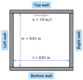
Cavity flow refers to a flow in a square container with a moving upper wall surface (i.e., the lid) and three stationary walls. Due to viscosity, the moving wall drives the fluid in proximity to move in the same direction until the stationary wall forms a jet impacting the lower wall and then forms a secondary vortex. On the one hand, the lid-driven cavity flow has a wide range of applications in the industry, such as the transient coating (short dwell coating) process [2], the ocean flow affected by the wind, and so on. On the other hand, the special case is that the BC is discontinuous [42] at the connection of the moving wall and the stationary side wall, which makes it judge the convergence of numerical methods. Thus, it is widely used to verify the accuracy of computational fluid mechanics software or numerical methods [14]. Therefore, the construction of the top lid-driven cavity flow data set is beneficial to study the ability of the neural network model to solve the flow problem.

Table 1. Operating parameters of the subset in the cavity flow problem.


BC	$u_{B} \in {1, 2, 3, \dots, 50} m / s$
Property	$ρ \in {0.1, 0.5, 1, 2, 3, \dots, 10} k g / m^{3}$
	$μ \in {10^{- 5}, 5 \times 10^{- 5}, \dots, 5 \times 10^{- 3}, 10^{- 2}} P a \cdot s$
Geometry	$l, w \in {0.01, 0.02, 0.03, 0.04, 0.05}$ m

In the dataset with the cavity flow, the baseline conditions are

ρ = 1 k g / m^{3}

μ = 10^{- 5} P a \cdot s

l = d = 0.01 m

u_{top} = 10 m / s

, where

ρ

and

μ

are the density and viscosity of the fluid, l and d are the length and width of the cavity, and

u_{top}

is the top wall movement velocity. 50 different cases are generated by varying

u_{top}

from

1 m / s

50 m / s

with a constant step size. 84 cases are generated varying the physical properties of the working fluid, with 12 different values of density and 7 values of viscosity. For the cases with different geometries, we choose different combinations of length and width from

{0.01, 0.02, 0.03, 0.04, 0.05}

. To have an appropriate scale of difference between the frames, we set the time step size to

Δ t = 0.1 s

3.3. Tube Flow

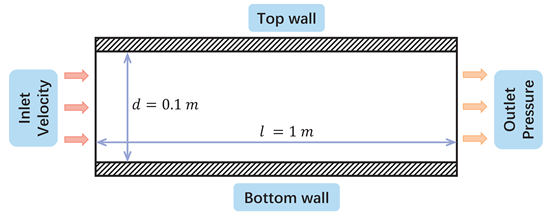
The tube flow refers to a water-air two-phase flow into the circular tube filling with air The boundary layer in the circular tube is one of the most common flows, which means that the viscosity resistance of the fluid on the near-wall surface is greater than the fluid in the bulk flow region. When the water flows into the round tube filled with air, we can clearly see that the flow is slow near the wall and fast in the center. Therefore, the construction of water-air laminar flow in a circular tube is beneficial to study the ability of the neural network structure to capture the two-phase interface and to learn the laminar boundary layer theory.

Table 2. Operating parameters of the subset in the tube flow problem.


BC	$u_{B} \in {0.1, 0.2, 0.3, \dots, 5} m / s$
Property	$ρ \in {10, 120, 320, \dots, 1000} k g / m^{3}$
	$μ \in {0.01, 0.12, 0.23, \dots, 1} P a \cdot s$
Geometry	$l \in {0.01, 0.05, 0.1, 0.3, 0.5} m$
	$d / l \in {1, 2, 5, 7.5, 10, 15, 20, 50, 75, 100}$

In the dataset of the tube flow, the baseline conditions are

ρ = 100 k g / m^{3}

μ = 0.1 P a \cdot s

u_{i n} = 1 m / s

d = 0.1 m

l = 1 m

, where

ρ

and

μ

are the density and viscosity of the fluid,

u_{i n}

is the inlet velocity (from the left), d and l is the diameter and the length of the circular tube. 50 cases were generated for different BCs, increasing the inlet velocity from

0.1 m / s

5 m / s

, with increments of

0.1 m / s

. 100 cases with different physical properties of the working fluid are generated, and the two-dimensional space of different densities and dynamic viscosity are shown in Table 3, where the density increases from

10 k g / m^{3}

1000 k g / m^{3}

with increments of

110 k g / m^{3}

, and viscosity increases from to and the viscosity increases from

0.01 P a \cdot s

1 P a \cdot s

with increments of

0.11 P a \cdot s

. For different geometries, the diameter of the circular tube is taken from

{0.01, 0.05, 0.1, 0.3, 0.5}

, and we choose five different ratios of diameter and length by making sure the length satisfies

0.1 \leq l \leq 10

. This results in 25 different geometries. To have an appropriate scale of difference between the frames, we set the time step size to

Δ t = 0.01 s

Table 3. Operating parameters of the subset in the dam flow problem.


BC	$u_{B} \in {0.05, 0.1, \dots, 1} \cup {1.02, 1.04, \dots 2} m / s$
Property	$ρ \in {0.1, 0.5, 1, 2, 3, \dots, 10} k g / m^{3}$
	$μ \in {10^{- 5}, 5 \times 10^{- 5}, \dots, 5 \times 10^{- 3}, 10^{- 2}} P a \cdot s$
Geometry	$h \in {0.11, 0.12, 0.13, 0.14, 0.15} m$
	$w \in {0.01, 0.02, \dots, 0.08, 0.09} m$

3.4. Dam Flow

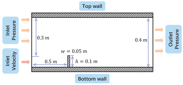
A dam is a barrier across flowing water that obstructs, directs, or slows down the flow. Meanwhile, sudden, rapid, and uncontrolled release of impounded water quickly causes a dam to burst [1]. To further understand the flow of water over the dam, we simplified it to the flow of water over a vertical obstacle. When the Reynolds number is low, the fluid is dominated by the viscous force and will flow vertically down the wall as it flows through the dam [35]. As the speed increases, the fluid is more affected by the inertial force, and a jet will be formed. Then the fluid falls to the boundary because of gravity and the collision with the boundary makes more reverse flow, which will hit the dam with a bigger velocity than the inlet. Therefore, the dam flow dataset is helpful in studying the learning ability of the model for flows subject to different viscous and inertial forces.

In the dataset of dam flow, the baseline conditions are

ρ = 100 k g / m^{3}

μ = 0.1 P a \cdot s

u_{i n} = 1 m / s

h = 0.1 m

w = 0.05 m

, where

ρ

and

μ

are the density and viscosity of the fluid,

u_{i n}

is the inlet velocity (from the left), h and w is the height and the width of the dam obstacle. The entire fluid domain is 1.5m long and 0.4m high. The inlet velocity boundary is close to the ground, with a total length of 0.1m, and 0.3m above it is the inlet pressure boundary. The barrier is located 0.5m from the entrance. 70 cases were generated for different BCs, increasing the inlet velocity from

0.05 m / s

1 m / s

with increments of

0.05 m / s

and from

1 m / s

2 m / s

with increments of

0.02 m / s

10 k g / m^{3}

1000 k g / m^{3}

with increments of

110 k g / m^{3}

, and viscosity increases from to and the viscosity increases from

0.01 P a \cdot s

1 P a \cdot s

with increments of

0.11 P a \cdot s

. 50 cases with different geometries are generated, increasing the height from

0.11 m

0.15 m

with increments of

0.01 m

and width from

0.01 m

0.09 m

with increments of

0.01 m

of dam obstacle. To have an appropriate scale of difference between the frames, we set the time step size to

Δ t = 0.1 s

3.5. Cylinder Flow

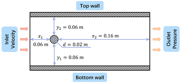
A flow around a cylinder is a typical boundary layer flow, which is commonly seen in the industry where water flows through bridges, the wind blows through towers, etc [41]. When the fluid with a large flow rate passes around the cylinder, the boundary layer fluid separates to form the reverse zone due to the combined effect of reverse pressure gradient and wall viscous force retardation. At a specific Reynolds number, the two sides of the cylinder periodically generate a double row of vortexes with opposite rotational directions and are arranged in a regular pattern. Through nonlinear interactions, these vortexes form a Karman vortex street. after nonlinear action. Therefore, the cylindrical flow dataset is important for examining the capability of neural networks in modeling periodic flows with obstacles.

In the dataset of the cylinder flow, the baseline conditions are

ρ = 10 k g / m^{3}

μ = 0.001 P a \cdot s

u_{i n} = 1 m / s

d = 0.02 m

x_{1} = y_{1} = y_{2} = 0.06 m

x_{2} = 0.16 m

, where

ρ

and

μ

are the density and viscosity of the fluid,

u_{i n}

is the inlet velocity (from the left), d is the diameter of the cylinder,

x_{1}, x_{2}, y_{1}, y_{2}

is the distance between the center of the cylinder and the left, right, top and bottom boundaries, respectively. 50 cases are generated for different BCs, increasing the inlet speed from

0.1 m / s

5 m / s

with increments of

0.1 m / s

. 115 cases are generated for the different physical properties of the fluid so that the Reynolds numbers are in the range of

[20, 1000]

. Table 4 shows some values of density and viscosity, but not all combinations are used because that results in Reynolds numbers outside of the target range. For different geometries, the distance from the cylinder to the upper and lower boundaries and the entrance is taken from

{0.02, 0.04, 0.06, 0.08, 0.1}

, the distance from the cylinder to the exit boundary is taken from

{0.12, 0.14, 0, 16, 0.18, 0.2}

, and the radius of the cylinder is taken from

{0.01, 0.02, 0.03, 0.04, 0.05}

. 20 cases are generated. To ensure an appropriate scale of difference between the frames, we set the time step size to

Δ t = 0.001 s

Table 4. Operating parameters of the subset in the cylinder flow problem.


BC	$u_{B} \in {0.1, 0.2, 0.3, \dots, 5} m / s$
Property	$\begin{matrix} ρ & \in {0.1, 0.2, \dots, 1} \cup {1.5, 2.5, \dots, 4.5, 5} \cup {6, 7, \dots, 9, 10} \\ \cup {20, 30, 40, \dots, 250} \cup {300, 400, 500} k g / m^{3} \\ μ & \in \{10^{- 4}, 5 \times 10^{- 4}, 10^{- 3}, 5 \times 10^{- 3}, 10^{- 2}\} P a \cdot s \end{matrix}$
Geometry	$d \in {0.01, 0.02, 0.03, 0.04, 0.05} m$
	$x_{1}, y_{1}, y_{2} \in {0.02, 0.04, 0.06, 0.08, 0.1} m$
	$x_{2} \in {0.12, 0.14, 0.16, 0.18, 0.2} m$

The problem datasets and the number of cases under different operating conditions are summarized in Table 5.

3.6. Data Generation

All the data in this paper are generated by ANSYS Fluent 2021R1. In order to calculate the viscosity term accurately, the laminar model is used for laminar flow and SST

k - ω

model for turbulent flow. All solvers used are based on pressure. We choose a Coupled Scheme for single-phase flow and SIMPLE for two-phase flow as a pressure-velocity coupling algorithm. The pressure equation uses the second-order interpolation method (the VOF model uses the PRESTO! Interpolation method), and the momentum equation adopts the second-order upwind method. The time term adopts the first-order implicit format and interpolation uses the least squares method. To capture the phenomenon of boundary layer separation at the near-wall surface, the size of the first layer mesh in the near-wall surface is encrypted to

10^{- 5} m

. To ensure the accuracy of the computational model and results, all computational models underwent grid-independent validation.

After discretizing the governing equations, the conservation equation of the universal variable

(Φ_{P})

at the grid element P can be expressed as:

\begin{matrix} a_{P} Φ_{P} = \sum_{n b} a_{n b} Φ_{n b} + b \end{matrix}

(3)

in which

a_{P}

is coefficient of the node of element P,

a_{n b}

is coefficients of neighbor nodes and b is the coefficient generated by constant term, source term and boundary condition. It defines the global scaling residual as:

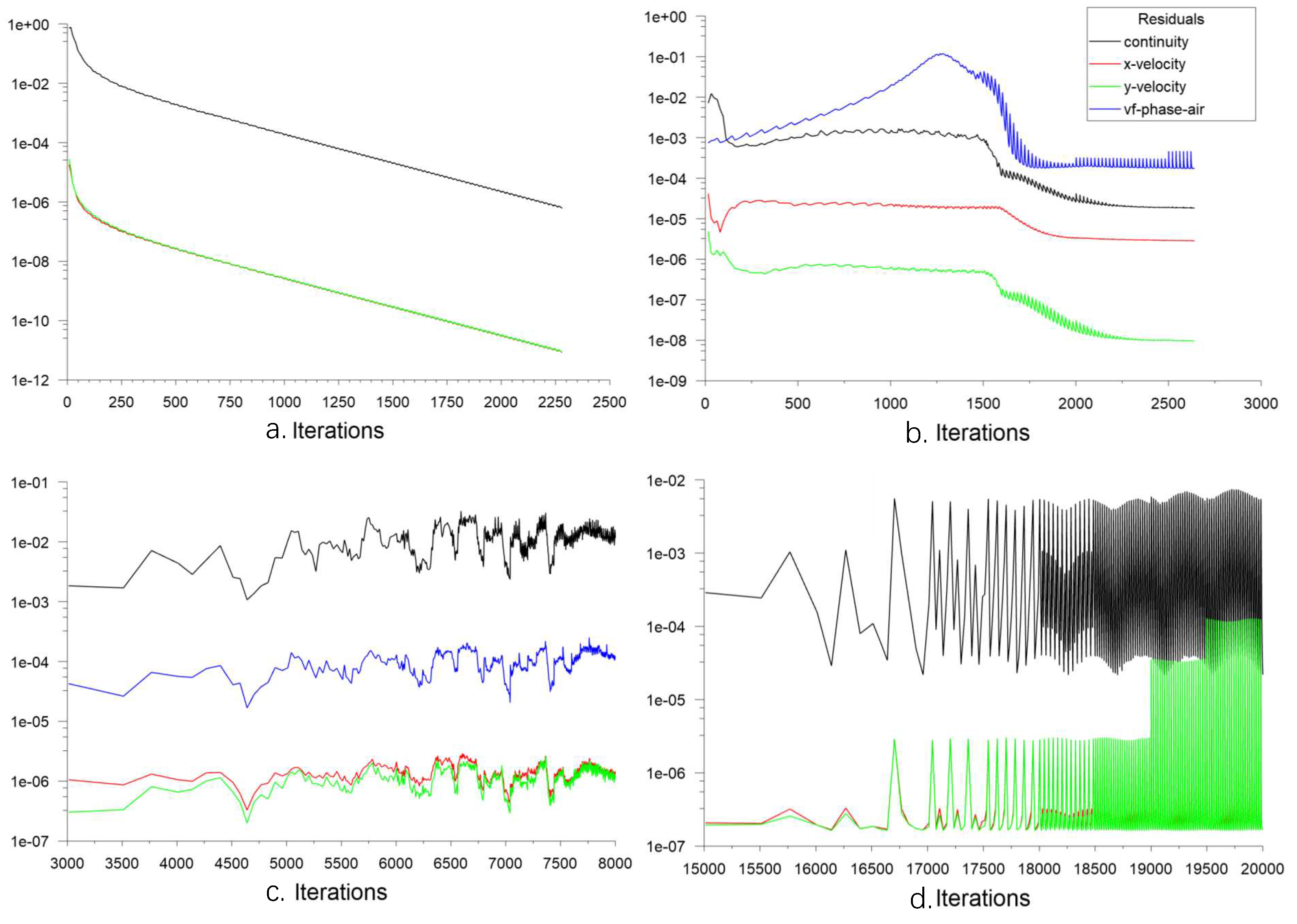
\begin{matrix} R^{Φ} = \frac{\sum_{c e l l s} | \sum_{n b} a_{n b} Φ_{n b} + b - a_{P} Φ_{P} |}{\sum_{c e l l s} | a_{P} Φ_{P} |} \end{matrix}

(4)

The residual represents the relative size of the total unbalance term in the computational domain, and is generally used to judge the convergence of the solution. The smaller the residual, the better the convergence. In this paper, the residual convergence condition of all terms is set to

10^{- 9}

, and the residuals in the final calculation results are shown as Figure 2. The residuals of the velocity terms are all at least

10^{- 6}

All generations are run with 30 solver processes on a CPU of AMD Ryzen Threadripper 3990X. The final generated data was interpolated to a grid size of

64 \times 64

3.6.1. Data Splitting

Each subset of data is split into training, validation, and test sets with a ratio of 8:1:1. The splitting unit is a case to ensure that the operating parameters in one set never appear in other sets.

4. Experiments

After generating the benchmark data, we use it to train popular data-driven neural networks that can be used for approximating the solutions to PDEs. To keep the number of experiments manageable, in the following discussions, unless stated otherwise, we have the models predict the velocity field. We believe that modeling other properties or components of the flow should not be too different.

We first define the learning objective of the neural network. Then, we give a brief description of the baselines we experimented on. After that, we explain the loss functions and hyperparameters used in the experiments.

4.1. Training Objectives

Most flow problems focus on solving the distribution of flow fields in the domain. Therefore, the objective of the neural networks is to approximate the following mapping within the domain

D = {(x, y, t) ∣ x \in [a, b], y \in [c, d], t \in [0, T]}

\begin{matrix} G : (Σ, Ω) \mapsto u \end{matrix}

(5)

where

Ω = (u_{B}, ρ, μ, d, l, w)

is the operating parameters, which include the BC

(u_{B})

, the physical properties

(ρ, μ)

, and the geometry S.

Σ

is the input function, which can be either the velocity field at a certain time (in autoregressive generation) or the spatiotemporal coordinate vector

(x, y, t)

(in the non-autoregressive model). u is the output function, which is the velocity field.

When using a neural network

f_{θ}

with parameters

θ

to approximate G, there are two approaches: non-autoregressive and autoregressive modeling.

Non-Autoregressive Modeling

In non-autoregressive modeling, the input function

Σ

is a query location

(x, y, t)

and the model directly outputs the solution at that position:

\begin{matrix} \hat{u} (x, y, t) = f_{θ} ((x, y, t), Ω) \in R \end{matrix}

(6)

Autoregressive Modeling

Autoregressive modeling, which is similar to traditional numerical methods, learns the mapping of a flow field from the current time step to the next time step. Therefore, it predicts the distribution of flow fields at each moment according to the temporal order:

\begin{matrix} \hat{u} (t) = f_{θ} (u (t - Δ t), Ω) \in R^{n \times m} \end{matrix}

(7)

where

\hat{u}

is the predicted value at time t, n and m are the height and width of the domain. In other words, the input function is

Σ = u (t - Δ t)

The learning goal is to find one

θ^{*}

that minimizes the loss function

L

on the training data

T

\begin{matrix} θ^{*} = arg max_{θ} L (u (x, y, t), \hat{u} (x, y, t)) & \forall x, y, t \in D, u \in T \end{matrix}

(8)

4.2. Baselines

We evaluate on CFDBench some popular and performant neural networks that have been applied to solve PDE in existing works. Although CFDBench can be used to evaluate both data-driven and physics-informed methods, our experiments are limited to the former. This is because most physics-informed methods enforce operating conditions through loss functions, and therefore require retraining on unseen conditions.

We can generally predict the flow in two manners: non-autoregressively or autoregressively. The former directly predicts the output function value at a query location specified in the input. The latter predicts the field at the next time step given the field at the current time step. The two kinds are not directly comparable, so we discuss them separately.

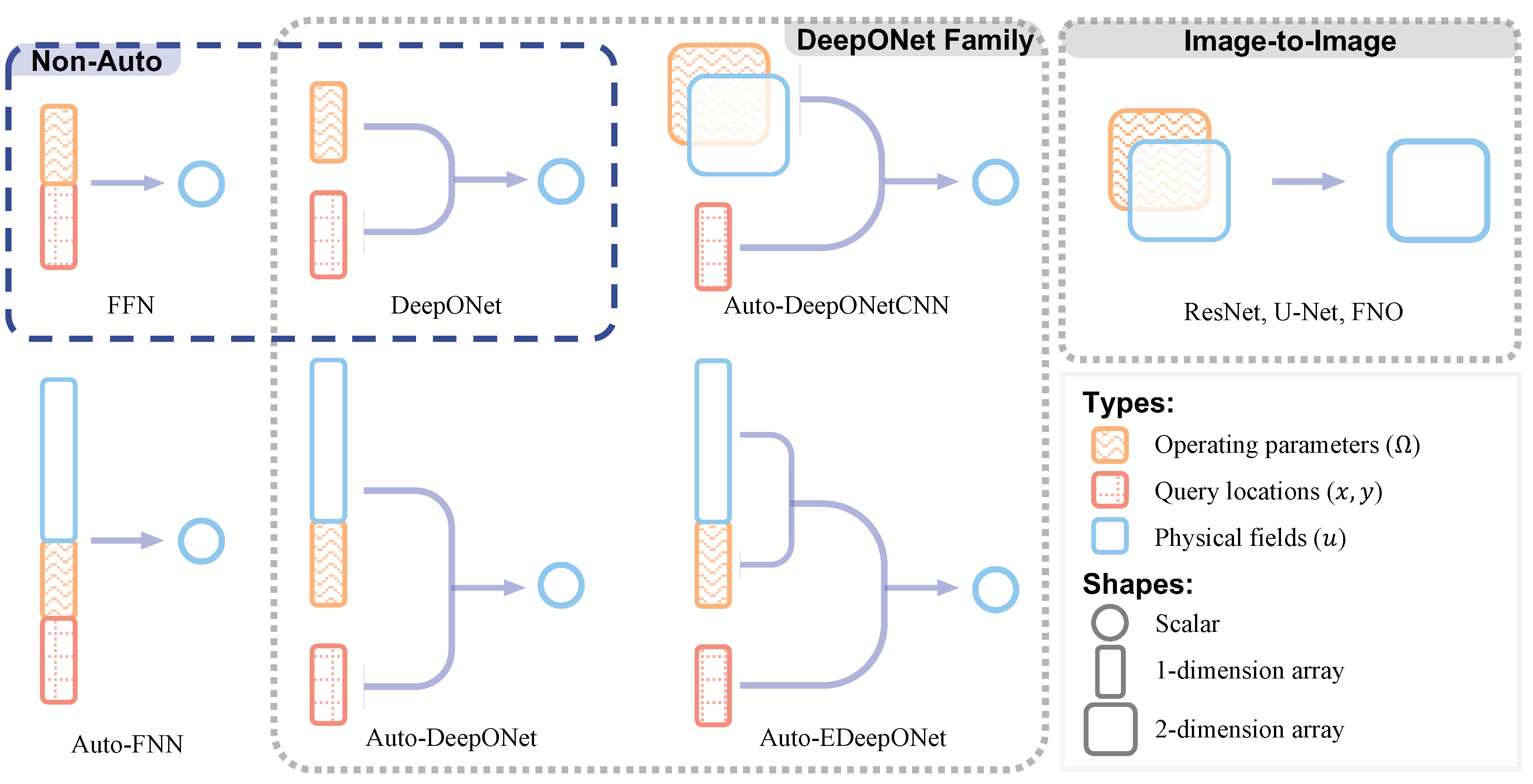
From the perspective of the model architecture, we can categorize them into three types: (1) FFNs, (2) the DeepONet family, and (3) image-to-image models. The first category simply concatenates all inputs into one vector and maps that to the prediction space with an FFN. The second category includes all variants of DeepONet [32]. The essence of this architecture is that the query location is independently encoded by a trunk net. This makes it possible to encode the input functions and other conditions without being limited to the shape or mesh of the output function domain and reuse that encoding to query the value of the output function at any location. The third category contains ResNet, U-Net, and FNO. They are the models that accept a n-dimensional array and output another n-dimensional array, which is the architecture that is commonly used for image-to-image tasks. Thus, we name this category image-to-image models. Table 6 compares all the baselines that we consider in this paper and Figure 3 figuratively illustrates the types and shapes of the input and output of each model.1

4.3. Non-Autoregressive Baselines

In non-autoregressive modeling, we refer to the operating condition

Ω

as the input function.

4.3.1. FNN

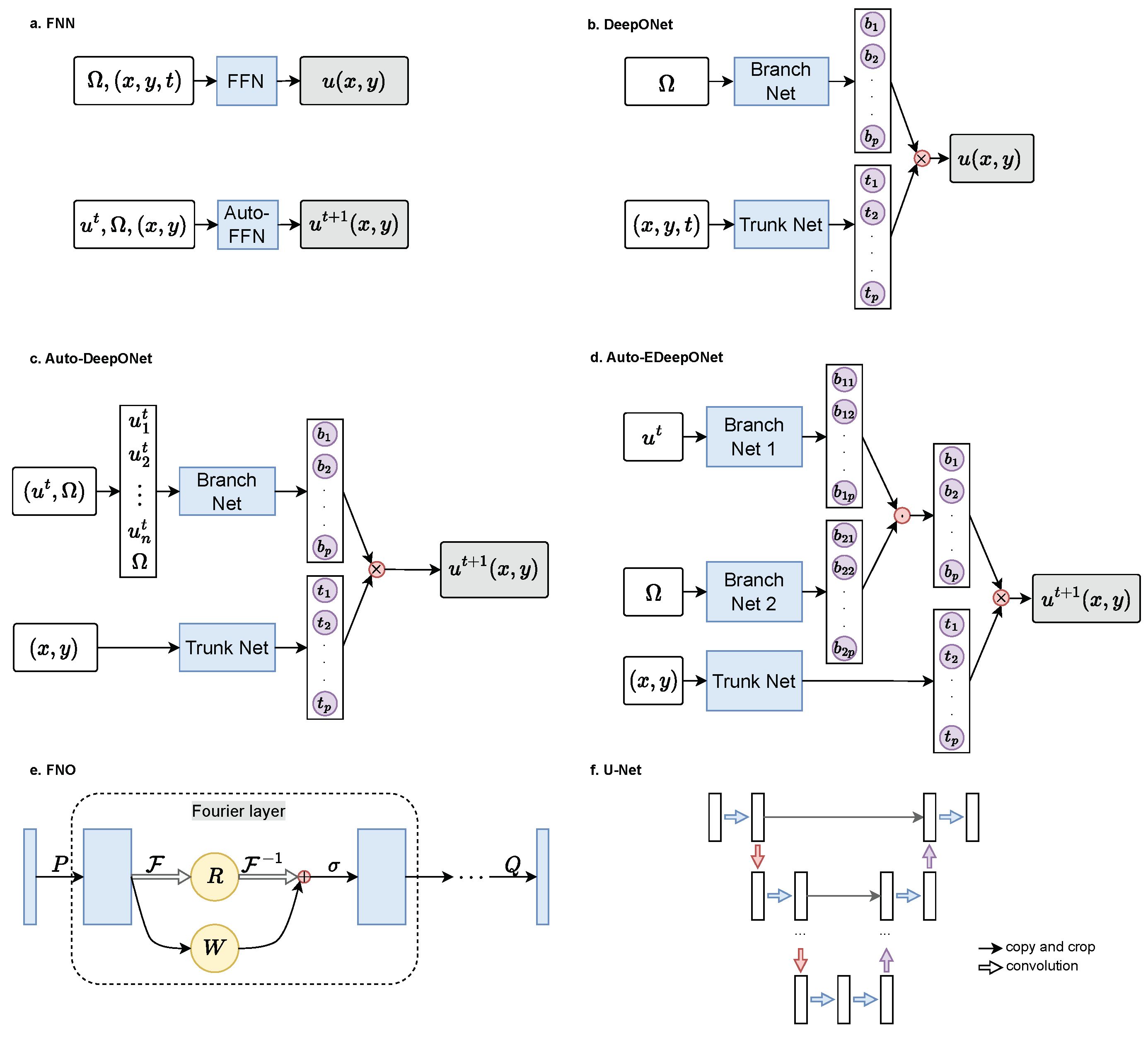
FNN is the simplest form of non-autoregressive modeling. The coordinates of the query location and the input function are simply concatenated into one vector, and fed to a chain of fully connected layers. Thus, the prediction is

\begin{matrix} \hat{u} (x, y, t) = f_{θ} (Ω | | (x, y, t)), \end{matrix}

where

| |

is the concatenation operator. This model is depicted in Figure 4a and it can be regarded as the data-driven version of PINN [36].

4.3.2. DeepONet

[32] have shown that by separating the encoding process of the input function and the query location can reduce error. They are encoded by two separate FFNs, the branch net and the trunk net. The outputs are aggregated by dot product to produce the final prediction:

\begin{matrix} \hat{u} (x, y, t) = f_{B} (Ω) \cdot f_{T} (x, y, t) + b, \end{matrix}

(9)

where

f_{B}

and

f_{T}

are the branch and trunk net, and

b \in R

is a trainable scalar that acts as the bias term. In other words, DeepONet is a specific case of FFN where each linear layer is cut in half, and each neuron can only see the operating parameters

Ω

or only the query coordinates

(x, y, t)

Furthermore, to improve the training speed of DeepONet, we can reuse the output of the branch net within each mini-batch. We sample

k = 1000

points in each frame as labels.

f_{B} (Ω)

is computed once, and each of the 1000 points

(x, y, t)

are dotted with

f_{B} (Ω)

before updating the model weights. Figure 4b illustrates the structure of DeepONet.

4.4. Autoregressive Baselines

Autoregressive is arguably more similar to traditional numerical solvers, where the model predicts the flow state at the next time step given the previous time step, i.e.,

f_{θ} : (u (t - Δ t), Ω) \mapsto u (t)

. Image-to-image models directly model

f_{θ}

, and different image-to-image models differ only in the implementation of

f_{θ}

4.4.1. Autoregressive FFN

The autoregressive FFN is similar to the non-autoregressive version. The input field, operating conditions, and the query location are all concatenated and fed to an FFN, which predicts the current field at the query location:

\begin{matrix} \hat{u} (x, y, t) = f_{θ} (u_{sample} | | Ω | | (x, y)), \end{matrix}

(10)

where

u_{sample}

refers to a list of field values sampled from u. This can be seen as a completely data-driven version of PINN [36]. Figure 4a depicts the structure of Auto-FFN.

4.4.2. Autoregressive DeepONet

We also consider modifying DeepONet to allow it to generate the solution autoregressively, and we name this model Auto-DeepONet.The structure is shown in Figure 4c. The input to the branch net (i.e., the input function) is

(u (t - Δ t), Ω)

where

u (t - Δ t)

is the last predicted velocity field and

Ω

is the operating condition parameters. The input to the trunk net is the spatial coordinates

(x, y)

of the query location, while the target output of the model is the value of the velocity field in the next time frame at

(x, y)

, i.e.,

u (x, y, t)

. The model is formulated as follows.

\begin{matrix} \hat{u} (x, y, t) = f_{B} (u_{sample} (t - Δ t) | | Ω) \cdot f_{T} (x, y) + b \end{matrix}

(11)

4.4.3. Autoregressive EDeepONet

EDeepONet (Enhanced DeepONet) [46] extends DeepONet’s architecture to consider multiple input functions. EDeepONet has one branch net for encoding each input function independently, and the branch outputs are aggregated by element-wise product. Since in autoregression, the DeepONet conditions on two inputs,

u (t - Δ t)

and

Ω

, we also evaluate the autoregressive version of, Auto-EDeepONet. The prediction is modeled as follows.

\begin{matrix} \hat{u} (x, y, t) = [f_{B 1} (u_{sample} (t - Δ t)) ⊙ f_{B 2} (Ω)] \cdot f_{T} (x, y) + b \end{matrix}

(12)

where ⊙ denotes the element-wise product.

In other words, EDeepONet is a specific case of DeepONet, where the branch net is split into two parts, each responsible for one input functions) and the neural links between each piece are removed (or deactivated by setting them to zero). This structure is illustrated in Figure 4d.

We do not evaluate the non-autoregressive version of EDeepONet because our preliminary experiments show that splitting

Ω

has no significant impact on the ability of the neural network. However, in autoregression, the input includes

u_{sample} (t - Δ t)

, which is much larger than

Ω

, and simply concatenating the two vectors may cause the neural to fail to learn dependence on

Ω

4.4.4. Autoregressive DeepONetCNN

We also experimented with CNN as the feature extractor for the input field called Auto-DeepONetCNN. This is almost the same as Auto-DeepONet, but the

f_{B}

is implemented with a CNN, because CNN may be better at extracting features from a lattice of a field. Since CNN requires a cuboid input, the input to the branch net needs to be

u (t - Δ t)

instead of

u_{sample} (t - Δ t)

. Similar to ResNet, U-Net, and FNO,

Ω

is appended to

u (t - Δ t)

as additional channels. The formulation is as follows.

\begin{matrix} \hat{u} (t) = CNN (u (t - Δ t), Ω) ⊙ f_{T} (x, t) + b \end{matrix}

(13)

4.4.5. ResNet

A residual neural network (ResNet) is a CNN with residual connections proposed by [18], and it has shown excellent performance on many computer vision tasks. Residual connectivity can effectively alleviate the degradation problem of the neural network when the depth increases, thus enhancing the learning ability of the model.2 The model can be formalized as follows.3

\begin{matrix} \hat{u} (t) & = {ResNetBlock}_{l} \circ \dots \circ {ResNetBlock}_{1} (x) & x = f_{i n} (u (t - Δ t), Ω) \end{matrix}

(14)

\begin{matrix} {ResNetBlock}_{i} (x) & = x + {CNN}_{i} (x) i = 1, \dots, l \end{matrix}

(15)

where

CNN (\cdot)

is a CNN network.

ResNet has many possible ways to put the ResNet blocks together, and this paper uses a string of residual blocks of the same size.

4.4.6. U-Net

U-Net [40] is a CNN with an encoder-decoder structure, which performs very well in numerous image segmentation and image-to-image translation tasks. The encoder realizes feature extraction and parameter reduction through down-sampling methods such as convolution (with larger striding) and pooling, and the decoder uses the feature encodings to produce an image through up-sampling and channel splicing, so as to achieve the purpose of image generation or segmentation. Compared to ResNet, the down-sampling of U-Net can reduce the number of parameters. Up-sampling can improve the globality of the convolution kernel because after up-sampling, a signal affects a larger region than without up-sampling. The structure of the U-Net used in this paper is illustrated in Figure 4f.

\begin{matrix} \hat{u} (t) & = UNet (u (t - Δ t), Ω) & \hat{y} & = f_{o u t} (y_{0}) \end{matrix}

(16)

\begin{matrix} x_{0} & = f_{in} (u (t - Δ t), Ω) & y_{0} & = {UpConv}_{1} (y_{1}, x_{0}) \end{matrix}

(17)

\begin{matrix} x_{1} & = {DownConv}_{1} (x_{0}) & y_{1} & = {UpConv}_{2} (y_{2}, x_{1}) \end{matrix}

(18)

\begin{matrix} ⋮ & ⋮ \end{matrix}

(19)

\begin{matrix} x_{l} & = {DownConv}_{l - 1} (x_{l - 1}) & y_{l} & = {UpConv}_{l} (y_{l + 1}, x_{l}) \end{matrix}

(20)

\begin{matrix} x_{l + 1} & = {DownConv}_{l} (x_{l}) & y_{l + 1} & = x_{l + 1} \end{matrix}

(21)

where

\begin{matrix} DownConv (x_{i})) & = Conv (DownSample (x_{i - 1})) \end{matrix}

(22)

\begin{matrix} UpConv (y_{i}, x_{j}) & = Conv (UpSample [y_{i + 1}] | | x_{i}) & i = 1, \dots, l, \end{matrix}

(23)

{Conv}_{i} (\cdot)

denotes a CNN,

UpSample (\cdot)

and

DownSample (\cdot)

denotes the up-sampling and down-sampling functions, l denotes the number of U-Net blocks, and

f_{i n} (\cdot)

and

f_{o u t} (\cdot)

denotes two trainable mappings. This architecture is shown in Figure 4f.

4.4.7. FNO

Fourier neural operator (FNO) [29] is a neural network that parameterizes the convolution kernel in Fourier space. It can learn the mapping of high-dimensional space and especially performs well in the problem of turbulent pulsation. The Fourier neural operator first raises the input function to a high-dimensional space through a shallow fully connected network and then approaches the target transform through the Fourier layer containing the Fourier transform and the inverse transform. The FNO has better globality than an ordinary CNN because any signal in the Fourier space affects the output on the entire spatial domain. Figure 4e shows the structure of FNO, and it can be formalized as follows.

\begin{matrix} \hat{u} (t) & = Q (h_{l + 1}) \end{matrix}

(24)

\begin{matrix} h_{i + 1} & = {FourierBlock}_{i} (h_{i}) = F^{- 1} [R_{i} (F [h_{i}])] + W_{i} (h_{i}) + h_{i} & i = 1, \dots, l \end{matrix}

(25)

\begin{matrix} h_{1} & = P (u (t - Δ t), Ω) \end{matrix}

(26)

where

F (\cdot)

denotes the Fourier transform,

P (\cdot)

Q (\cdot)

W_{i} (\cdot)

are ordinary convolutional layers, and

R_{i} (\cdot)

is a

1 \times 1

convolutional layer.

It is worth mentioning that, in the original paper of FNO [29], the input includes multiple time steps before the current time step, which provides additional information about the flow’s state and may make inference easier. However, this limits the usability of the method. Therefore, in this work, we only consider the scenario where the input contains no more than one frame.

4.5. Conditioning on Operating Parameters

Most existing works on neural operators keep the operating parameters (

Ω

) constant, and the input function, which is the IC, is the only input to the operator. In contrast, CFDBench considers varying the operating parameters while keeping the IC constant. Consequently, we need to make appropriate modifications to existing neural models for PDEs such that the predictions can be conditioned on the operating parameters.

For the autoregressive models, we treat the problem as a conditional image-to-image translation task, where the velocity field at the previous moment

u (x, y, t - Δ t)

is the input image, the velocity field at the current moment

u (x, y, t)

is the target image, and the operating condition parameters

Ω

are the condition. For simplicity, we add

Ω

to the input as additional channels, one channel for each parameter. In this work, there are 5 parameters in

Ω

, so the input at position

(x, y)

(u (x, y), u_{B}, ρ, μ, h, w)

where

h, w

are the height and width. For the flow around a cylinder, the model also needs to know the location and shape of the obstacle. To this end, we add a mask channel where 0 indicates obstacles at that position and 1 indicates no obstacles.

4.6. Loss Functions

During training, we use the normalized mean squared error (the NMSE defined below) as the training loss function to ensure that the model would prioritize minimizing the difference for labels with smaller absolute values.4 For evaluating, we also report the following three kinds of error values for comprehensiveness. We denote the label value with

Y

and the predicted value with

\hat{Y}

Mean Square Error (MSE)

\begin{matrix} MSE = \frac{1}{n} \sum_{i = 1}^{n} {(Y_{i} - \hat{Y_{i}})}^{2} \end{matrix}

(27)

Normalized Mean Square Error (NMSE)

\begin{matrix} NMSE = \frac{\sum_{i = 1}^{n} {(Y_{i} - \hat{Y_{i}})}^{2}}{\sum_{i = 1}^{n} Y_{i}^{2}} \end{matrix}

(28)

Mean Absolute Error (MAE)

\begin{matrix} MAE = \frac{1}{n} \sum_{i = 1}^{n} | Y_{i} - \hat{Y_{i}} | \end{matrix}

(29)

As we will show with experiments in Section 5, one method may perform better than another method in terms of one metric, but perform worse in terms of another metric. Therefore, it is important for practitioners to select one or multiple metrics that best reflect their interests.

4.7. Hyperparameter Search

The performance of the methods is dependent on the hyperparameters such as learning rate, number of training epochs, etc. Because our problem setting is significantly different from existing works, the optimal hyperparameters of each baseline model are likely very different from the ones found by the authors. We perform a hyperparameter search of the baseline models using the PROP subset of the cavity flow problem (84 different flows).

A more detailed description of the hyperparameter search process can be found in the Appendix. In summary, to make the methods comparable, we generally want to keep the number of parameters to be roughly the same.5 For ResNet, U-Net, and FNO, we try different depths and numbers of hidden channels. We also experiment with new ways to inject operating parameters. For FNN and variants of DeepONets, we try different widths and depths of the hidden linear layers. Additionally, the learning rate is selected individually for each method based on the validation loss, and we always train until convergence.

4.7.1. ResNet

For ResNet, we conducted a hyperparameter search on the depth d (i.e., the number of residual blocks) and hidden dimension h (i.e., the number of channels of the output of each residual block). We found that ResNet’s ability to learn from flow problems is poor, and it quickly becomes unable to converge when d and h increase6. The setting with the lowest validation loss is

d = 4

and

h = 16

, which we used to train on the data of flow in the tube, and the test loss is shown in Table 7. The result shows that ResNet’s performance is generally slightly worse than the identity transformation. One plausible explanation for this is that ResNet is poor at modeling global dependencies, i.e., the input signal at any point after one convolution layer with a

k \times k

kernel can only spread around the original position within its neighboring

k \times k

range. Therefore, we do not consider ResNet in further discussions below.

4.8. Other Details

For autoregressive models, we always train the model on one forward propagation, while for non-autoregressive models to train on randomly sampled query points on the entire spatiotemporal domain. We tune the learning rate on the cavity PROP subset, and always have it decay by a factor of 0.9 every 20 epochs, which we empirically found to be effective. One may get better performance by tuning more hyperparameters, such as trying different learning rate schedulers and tuning them on the entire dataset. However, that is prohibitively expensive considering the size of the dataset.

All methods were implemented using PyTorch deep learning framework, and all experiments were executed on one local computer with one RTX 3060 GPU. Most results are the average of three runs with different random seeds.

5. Results

Our analysis of the experimental results commences with the prediction of the flow field distribution at a singular time step, subsequently progressing to the autoregressive inference of multiple sequential time steps. To evaluate the predictive capabilities, we conduct a comparative assessment of both non-autoregressive and autoregressive models. Additionally, we provide a comparative analysis of the computational power consumption associated with each of these models.

5.1. Single Step Prediction

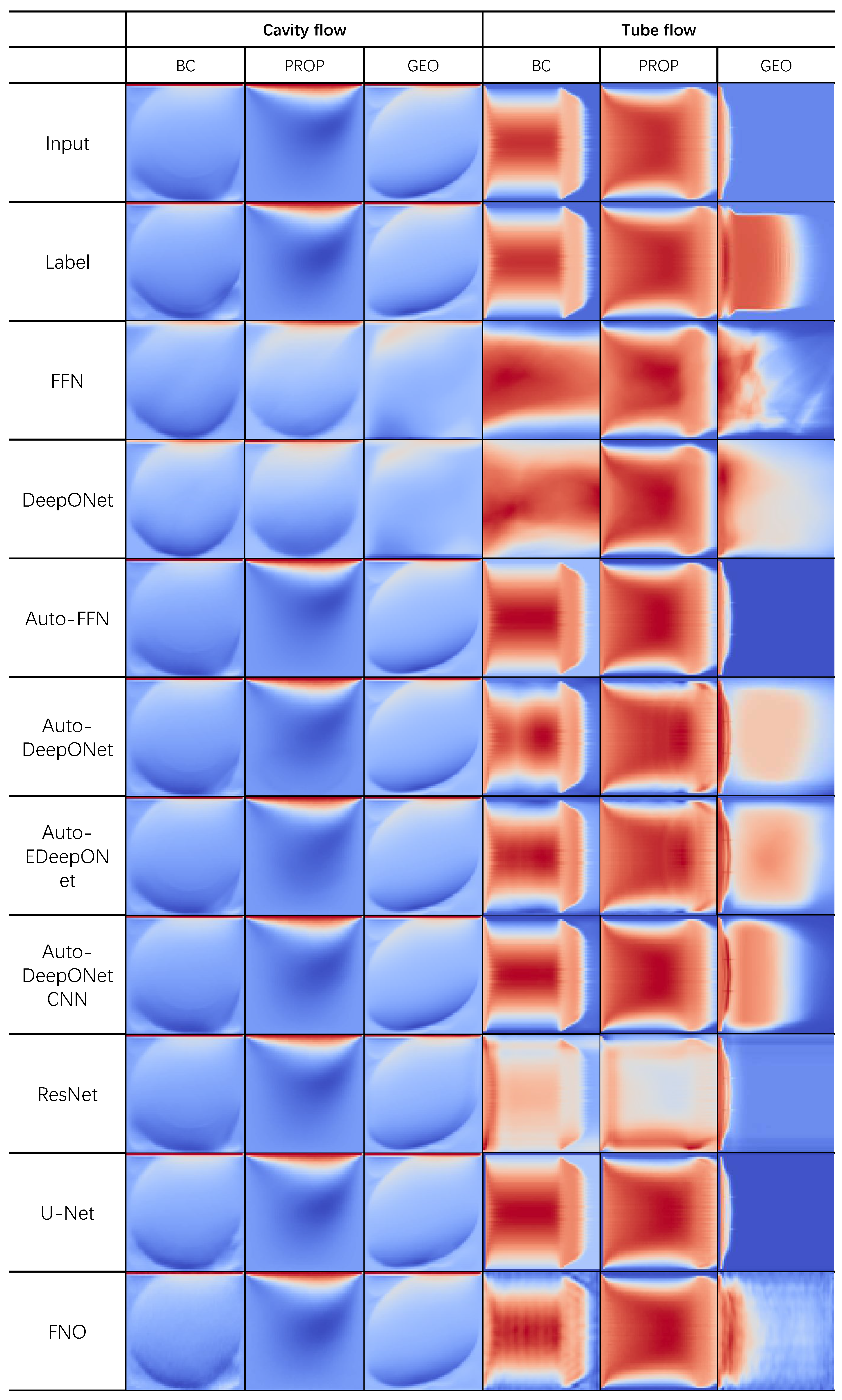
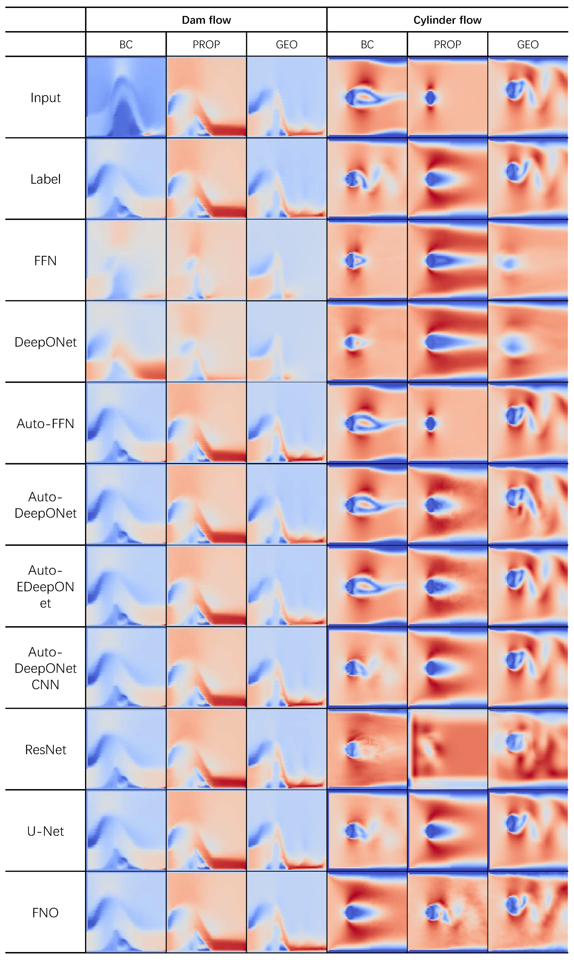
Figure 5 and Figure 6 show the predicted velocity field of all baseline models on the three subsets of the four flow problems in CFDBench. From top to bottom, the first row is the input, the second row is the label, and the following are the predictions of non-autoregressive and autoregressive models. We find, in general, that the baseline models perform relatively well on cavity flow and dam flow while struggling on tube flow and cylinder flow, especially for non-autoregressive models.

It is important to recognize the difference between autoregressive and non-autoregressive models when analyzing the result. The task of the non-autoregressive model is to directly produce the value of the output function at a designated query location in the entire spatiotemporal domain. This should be significantly more difficult than the autoregressive model, which only needs to learn the mapping from the field at the previous time frame to the field at the current time frame.

Also, the autoregressive models require that the input and output functions be represented with a grid, which limits their flexibility and may result in loss of information on regions where the field value changes sharply for small spatial changes. Furthermore, the non-autoregressive model has better mesh-independence, because the model can output the predicted value of the output function at any location. This has great significance for the study of many topographic complex problems. In addition, non-autoregressive inference may be much more efficient 7 because it can predict values at any time frame while autoregressive models need to propagate one time step at a time. In summary, the autoregressive and non-autoregressive models cannot be directly compared against each other, and non-autoregressive inference is generally much faster at long-range prediction and is significantly more difficult.

5.1.1. Non-Autoregressive Modeling

Table 8 shows the test results of FFN and DeepONet on the four problems and their corresponding seven subsets in CFDBench. Contrary to the observations by [32], we find that FNN generally has a better generalization ability compared to DeepONet in most cases. In some cases, the error of FNN is several orders of magnitude smaller than that of DeepONet. In contrast, in DeepONet’s best cases, it still only has a marginal accuracy gain over FFN. However, we believe this is not surprising because DeepONet is one specific case of FFN.

We also observe the PROP subset is generally easier than other subsets. This is likely because physical properties affect the velocity less than other operating parameters, making train-test domain gap smaller. With varying BCs and geometries, DeepONet suffers from severe overfitting, producing fields with little resemblance to the labels. With varying BCs, it is prone to show the velocity distribution in a steady state while with varying geometries, it tends to behave as identity transformations.

5.1.2. Autoregressive Modeling

Figure 7 shows the test NMSE of the autoregressive models on the four flow problems (with all cases), this serves as a comprehensive summary of the performance of the autoregressive baselines. The complete result of our experiments is listed in Table 10, which contains the test NMSE, MSE, and MAE of each autoregressive model on each of the seven subsets of the four problems in CFDBench.

In general, Auto-FFN and autoregressive models from the DeepONet family are at best slightly better than the identity transformation, which means they often learn to output the input as their predictions.

In cavity flow and tube flow, U-Net demonstrates superior performance due to its encoding-decoding structure in the spatial domain, which enables it to capture sharp changes in the velocity field more effectively. On the other hand, the MSE of U-Net and FNO is small while the MAE is large. This is because the velocities have generally small absolute values (

u < 1

), and the relative error is large when the absolute error is small.

In dam flow prediction, the DeepONet family generally prevails while the non-convergence phenomenon is observed in FNO (FNO’s result is excluded from the bar chart because the error is too large). The presence of gravity as a dominant physical force in dam flow suggests that the DeepONet family may be more effective in handling PDEs with source terms.

Both image-to-image models perform the best in the cylinder flow (

MSE \sim 10^{- 5}

MAE \sim 3 \times 10^{- 3}

), and in this dataset, FNO is better than U-Net. We conjecture this is because FNO is endowed with an ability to extract the characteristics of the periodic vortex more effectively by learning in the frequency domain.

For the tube flow problem, U-Net’s predictions have horizontal stripe noises while FNO manifests vertical pattern noise at

t = 0

. For the cylinder flow problem, we can see from the prediction that although FNO’s test loss is very low, it produces visible noises. This is because, in FNO, high frequencies are discarded to reduce the computational cost, as a result, it struggles to model flat regions and sharp changes. This also implies that the loss functions we have considered (which are also used in many previous works) may not be good at capturing all the artifacts of various methods.

5.2. Multi-Step Prediction

One important characteristic of traditional numerical methods is that they can extrapolate to any time points through an arbitrary number of forward propagation steps (provided that the iterative process converges). Consequently, it is desirable for data-driven deep learning methods to effectively generalize to time steps beyond those encountered during the training phase and predict the field at any time step. For non-autoregressive models, we can simply query points beyond the temporal range of the training distribution, but for autoregressive models, since predictions depend on the previous predictions, errors may accumulate over multiple forward propagation steps [3].

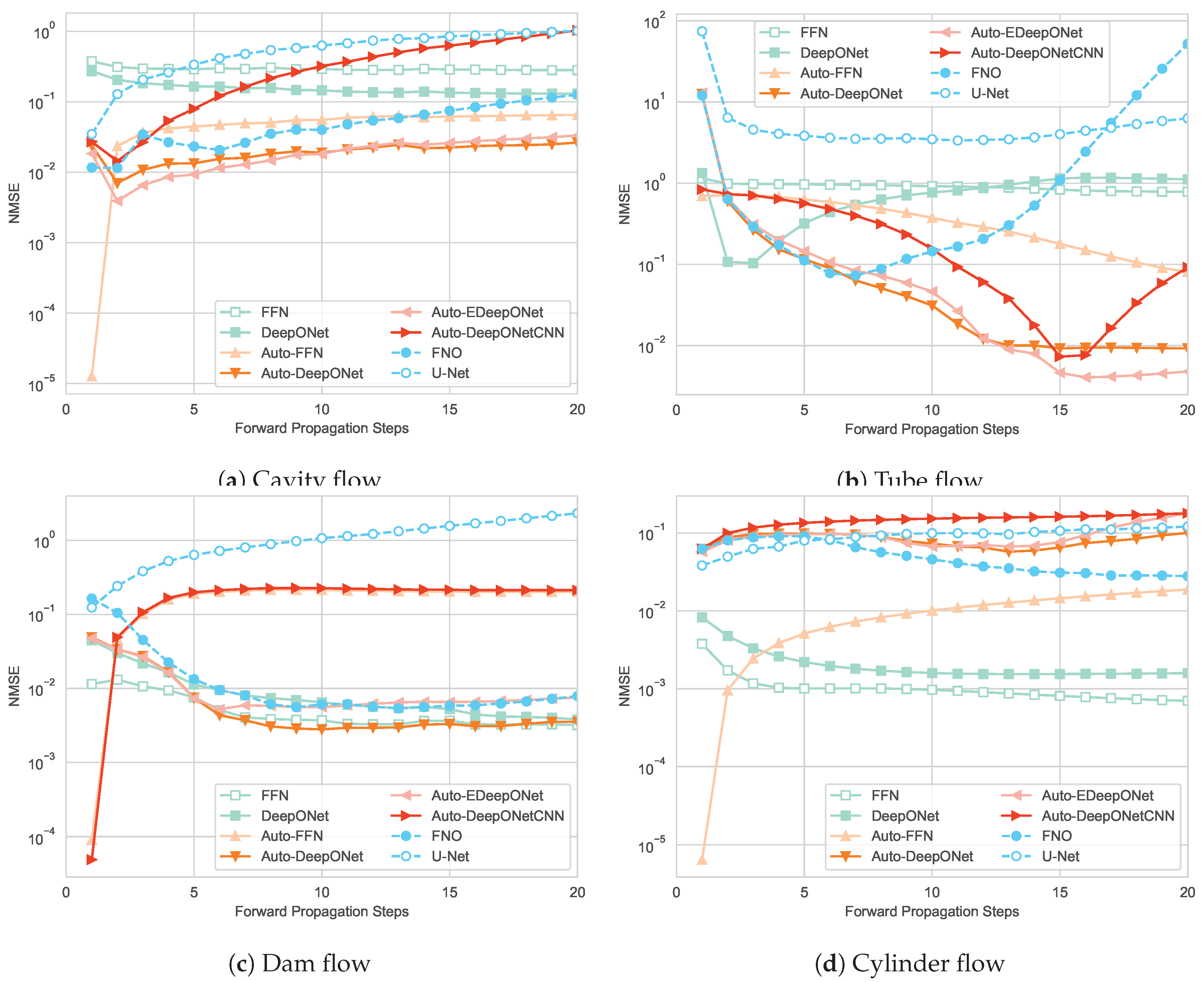
Figure 8 illustrates the errors of the baseline models by propagating from the IC (the velocity field at

t = 0

) with respect to different time steps. As expected, the errors of non-autoregressive models are stable with respect to the time step. In fact, with the exception of DeepONet in tube flow, non-autoregressive models generally have lower errors at later time points. This is because the change in the velocity field in earlier time steps is more drastic, which is more challenging to predict.

Concerning autoregressive models, in every problem, certain models exhibit significant error accumulation. One illustrative example is observed in the tube flow problem, where FNO’s error increases by 100 times within just 15 forward propagation steps. This adheres to our intuition. Perhaps surprisingly, in some cases, the errors of autoregressive models can decrease over time, which means that the prediction may have a lower error than the input itself. In other words, some autoregressive models are able to utilize the operating conditions to correct themselves. Another observation is that models with convolutional layers, i.e., U-Net, FNO, and Auto-DeepONetCNN, are more prone to error accumulation than other baselines. One possible explanation is that convolutional layers treat the features at different locations the same way, and despite adding the coordinates of each input point as additional channels, they are still worse than fully connected layers that have one set of weights dedicated to processing every input point.

Mitigating error accumulation is an active research direction and is out of the scope of this paper. One approach, suggested by [3], is to train multiple models with varying step sizes. An alternative strategy involves imposing physical constraints on the model, effectively rendering it “physics-informed”.

5.3. Computational Cost

For more complex flow problems, traditional numerical methods can be very expensive in terms of computational cost, often requiring days and even months to run simulations. It has been shown that deep learning methods can be multiple orders of magnitude faster than numerical methods [3,29,32], which is one of the primary advantages of data-driven methods [36].

Different from traditional numerical methods, deep learning methods also involve a training procedure, which can be very time-consuming, and a set of parameters that can be very memory-consuming. Thus, we need to consider these two aspects in addition to the inference time. We measured the computational cost of each baseline model in terms of time and memory usage during training and inference time. The result is listed in Table 9. The models are implemented with PyTorch and executed using GPU. The statistics for training are measured with a batch size of 32, and for inference, we use a batch size of 1. The experiment was conducted with one computed with one i7-12700F CPU and one RTX 3060 GPU.

From the result, we see that different models have very different computational costs, especially during training. Auto-FFN is around 21 times slower than Auto-DeepONet in training, despite having only double the number of parameters and no significant difference in prediction error. This is intuitive because as mentioned in Section 4.3.2, by reusing the output of the branch net within one mini-batch, DeepONet can significantly improve the training efficiency. Another important observation from this result is that autoregressive models generally have many more parameters compared to non-autoregressive models, but the two kinds of models have comparable training computational costs. This is because autoregressive baselines predict the entire output function with one forward pass, while non-autoregressive baselines predict each data point of the output function one by one.

On the other hand, during inference, the time needed for the models to perform one forward propagation (or one query for non-autoregressive models) is very similar, all within the range of 5 to 10 ms. This is much faster than the numerical method employed for the generation of this dataset, which takes around 1 second for every frame.

Table 10. The main results of autoregressive models on CFDBench on one forward propagation.

Problem 1: Cavity Flow
Method	(1) PROP	(2) BC	(3) GEO	(4) P+B	(5) P+G	(6) B+G	(7) All
Test NMSE
Identity	0.0008949	0.0006532	0.0073354	0.0026440	0.0012782	0.0019072	0.0014130
Auto-FNN	0.0008947	0.0006536	0.0073358	0.0026441	0.0012785	0.0019086	0.0014138
Auto-DeepONet	0.0008465	0.0006478	0.0071480	0.0025767	0.0012198	0.0019119	0.0013954
Auto-EDeepONet	0.0008953	0.0006539	0.0239769	0.0026405	0.0050122	0.0096511	0.0014756
Auto-DeepONetCNN	0.0007973	0.0006152	0.0033303	0.0016539	0.0009240	0.0011091	0.0010203
FNO	0.0004622	0.0006068	0.0097830	0.0006725	0.0015670	0.0019072	0.0005058
U-Net	0.0002815	0.0001159	0.0056645	0.0001383	0.0008825	0.0009481	0.0004166
Test MSE
Identity	0.0044942	0.0546373	0.0180946	0.0990002	0.0045866	0.0714307	0.0641640
Auto-FNN	0.0044936	0.0546386	0.0180943	0.0990127	0.0045873	0.0714420	0.0641692
Auto-DeepONet	0.0042624	0.0536015	0.0179865	0.0976493	0.0044118	0.0710621	0.0638475
Auto-EDeepONet	0.0044994	0.0547824	0.0669539	0.0989851	0.0156476	0.0950095	0.0644919
Auto-DeepONetCNN	0.0043076	0.0531823	0.0125515	0.0920075	0.0043748	0.0709266	0.0632696
FNO	0.0021805	0.0144506	0.0248771	0.0212877	0.0039921	0.0517444	0.0176914
U-Net	0.0044942	0.0083046	0.0118261	0.0064567	0.0017226	0.0210355	0.0158059
Test MAE
Identity	0.0181955	0.0506039	0.0297850	0.0850075	0.0181359	0.0564395	0.0546747
Auto-FNN	0.0182054	0.0507490	0.0298784	0.0854521	0.0183282	0.0570768	0.0552039
Auto-DeepONet	0.0192833	0.0540527	0.0327312	0.0814217	0.0198544	0.0663280	0.0566274
Auto-EDeepONet	0.0200762	0.0591863	0.1748586	0.0869751	0.0522350	0.0814745	0.0600075
Auto-DeepONetCNN	0.0210971	0.0542496	0.0222548	0.0792672	0.0201459	0.0571482	0.0584715
FNO	0.0164622	0.0503310	0.0570261	0.0512820	0.0272561	0.0941030	0.0569002
U-Net	0.0103330	0.0001159	0.0328206	0.0422648	0.0155698	0.0325585	0.0319145
Problem 2: Tube Flow
Test NMSE
Identity	0.1081580	0.1001696	0.0763603	0.1089607	0.0976491	0.1122125	0.1111430
Auto-FNN	0.0926980	0.1363334	0.0712057	0.1032522	0.0912989	0.1062881	0.1056823
Auto-DeepONet	0.0579279	0.0587133	0.0582056	0.0627424	0.0642253	0.0652362	0.0647747
Auto-EDeepONet	0.0523948	0.0849620	0.0577905	0.0833847	0.0641345	0.0860665	0.0778912
Auto-DeepONetCNN	0.0366433	0.0588061	0.0327204	0.0559905	0.0399490	0.0696541	0.0548516
FNO	0.0003789	0.0374976	0.0295622	0.0053018	0.0272909	0.0207228	0.0053062
U-Net	0.0018705	5.0228938	0.0291472	0.0111089	0.0118453	0.0190382	0.0031894
Test MSE
Identity	0.0317068	0.3432079	0.0298840	0.1495200	0.0287833	0.3478090	0.1642216
Auto-FNN	0.0279299	0.3017316	0.0280562	0.1298233	0.0259540	0.3374500	0.1554814
Auto-DeepONet	0.0169327	0.1229224	0.0223923	0.0635457	0.0189828	0.1395774	0.0723492
Auto-EDeepONet	0.0165697	0.2007642	0.0209080	0.0929376	0.0175065	0.2476731	0.0973665
Auto-DeepONetCNN	0.0268636	0.2177070	0.0266211	0.1133375	0.0248359	0.2599603	0.1031608
FNO	0.0001121	0.0025932	0.0120422	0.0007641	0.0057142	0.0123058	0.0012725
U-Net	0.0007242	0.3389257	0.0132874	0.0072537	0.0026152	0.0142700	0.0012903
Test MAE
Identity	0.0762089	0.1662700	0.0577343	0.1201217	0.0673662	0.1670072	0.1198109
Auto-FNN	0.1157967	0.2040521	0.0699715	0.1559224	0.1017113	0.2031115	0.1568468
Auto-DeepONet	0.0764206	0.1481193	0.0634907	0.1215821	0.0713417	0.1534080	0.1195835
Auto-EDeepONet	0.0754687	0.1766330	0.0685437	0.1341049	0.0691925	0.1905831	0.1323233
Auto-DeepONetCNN	0.1044903	0.2373263	0.0796258	0.1626967	0.0888877	0.2177044	0.1347066
FNO	0.0064773	0.0363909	0.0608122	0.0182902	0.0318654	0.0558519	0.0238839
U-Net	0.0139124	0.4283762	0.0431357	0.0349704	0.0169491	0.0526696	0.0181517
Method	(1) PROP	(2) BC	(3) GEO	(4) P+B	(5) P+G	(6) B+G	(7) All
Test NMSE
Identity	0.0019018	0.0039803	0.0065650	0.0020840	0.0041362	0.0056979	0.0031620
Auto-FNN	0.0018699	0.0039597	0.0065501	0.0020618	0.0041344	0.0056924	0.0031543
Auto-DeepONet	0.0016760	0.0036014	0.0064154	0.0019039	0.0039516	0.0055705	0.0030798
Auto-EDeepONet	0.0017231	0.0037461	0.0052787	0.0018735	0.0035536	0.0048973	0.0027361
Auto-DeepONetCNN	0.0018616	0.0039617	0.0065470	0.0020625	0.0041093	0.0057000	0.0031518
FNO	0.0266296	0.0524766	0.0154634	0.1206019	0.0307598	0.0314159	0.0636001
U-Net	0.0019239	0.0040659	0.0067332	0.0021257	0.0043181	0.0058265	0.0032407
Test MSE
Identity	0.0011082	0.0048598	0.0015390	0.0016745	0.0013234	0.0035683	0.0016937
Auto-FNN	0.0010898	0.0048156	0.0015359	0.0016551	0.0013186	0.0035535	0.0016800
Auto-DeepONet	0.0009789	0.0044238	0.0015048	0.0015351	0.0012433	0.0034572	0.0016390
Auto-EDeepONet	0.0010059	0.0045758	0.0012384	0.0014951	0.0011442	0.0031783	0.0014936
Auto-DeepONetCNN	0.0010854	0.0048134	0.0015349	0.0016510	0.0013099	0.0035586	0.0016810
FNO	0.0138105	0.0255943	0.0038784	0.0259257	0.0131788	0.0188826	0.0202863
U-Net	0.0011090	0.0048536	0.0015478	0.0016708	0.0013723	0.0035743	0.0017016
Test MAE
Identity	0.0083432	0.0137022	0.0058706	0.0087752	0.0072361	0.0105381	0.0082023
Auto-FNN	0.0075868	0.0135726	0.0070825	0.0079549	0.0076244	0.0105358	0.0082106
Auto-DeepONet	0.0064191	0.0127207	0.0076071	0.0072435	0.0065346	0.0098888	0.0072718
Auto-EDeepONet	0.0069405	0.0124701	0.0060389	0.0080457	0.0062325	0.0100111	0.0070318
Auto-DeepONetCNN	0.0073756	0.0134733	0.0063454	0.0082490	0.0069973	0.0108240	0.0080630
FNO	0.0878391	0.1118927	0.0332420	0.1143100	0.0755819	0.0788372	0.1016557
U-Net	0.0088548	0.0146514	0.0072130	0.0094619	0.0096587	0.0111258	0.0092133
Problem 4: Cylinder Flow
Test NMSE
Identity	0.0077999	0.0134142	0.0337257	0.0140363	0.0166764	0.0168646	0.0156948
Auto-FNN	0.0077977	0.0134795	0.0337259	0.0140332	0.0166751	0.0168684	0.0156955
Auto-DeepONet	0.0077462	0.0133213	0.0337149	0.0139771	0.0166488	0.0168484	0.0156741
Auto-EDeepONet	0.0064475	0.0125065	0.0337160	0.0138407	0.0158704	0.0168613	0.0156335
Auto-DeepONetCNN	0.0077035	0.0131733	0.0337303	0.0143524	0.0166459	0.0172999	0.0160131
FNO	0.0000055	0.0000221	0.0025348	0.0000184	0.0008809	0.0011412	0.0000178
U-Net	0.0000482	0.0002006	0.0014008	0.0000140	0.0004029	0.0007282	0.0000216
Test MSE
Identity	0.0085652	0.1510596	0.0391798	0.0495286	0.0189442	0.0988010	0.0754044
Auto-FNN	0.0085629	0.1510848	0.0391801	0.0495232	0.0189429	0.0988837	0.0754104
Auto-DeepONet	0.0085082	0.1492194	0.0391674	0.0493322	0.0189148	0.0981404	0.0753445
Auto-EDeepONet	0.0071054	0.1370049	0.0391690	0.0480996	0.0180690	0.0987495	0.0743118
Auto-DeepONetCNN	0.0084855	0.1467647	0.0392012	0.0493385	0.0189119	0.1009318	0.0751691
FNO	0.0000059	0.0000576	0.0030180	0.0000280	0.0010334	0.0013663	0.0000274
U-Net	0.0000517	0.0019469	0.0016252	0.0000391	0.0004649	0.0016478	0.0000549
Test MAE
Identity	0.0429706	0.1702698	0.1164363	0.0904745	0.0689821	0.1223419	0.1090931
Auto-FNN	0.0435852	0.1716940	0.1165288	0.0909219	0.0692674	0.1228507	0.1091991
Auto-DeepONet	0.0434741	0.1728876	0.1167489	0.0912146	0.0691589	0.1242880	0.1095553
Auto-EDeepONet	0.0430859	0.1663353	0.1165038	0.0903266	0.0681725	0.1224469	0.1095621
Auto-DeepONetCNN	0.0429322	0.1721080	0.1170427	0.0907547	0.0691550	0.1252522	0.1090919
FNO	0.0012435	0.0043508	0.0317458	0.0028028	0.0149799	0.0190607	0.0030647
U-Net	0.0040814	0.0240380	0.0251834	0.0027415	0.0076716	0.0192060	0.0030971

6. Conclusions

We introduce CFDBench, a large-scale and comprehensive benchmark for evaluating deep learning methods in fluid dynamics. CFDBench includes four archetypal flow scenarios, namely: (1) the lid-driven square cavity flow, (2) laminar boundary layer flow, (3) flow resulting from a dam break, and (4) flow around a cylindrical obstacle. Each problem contains seven subsets, each corresponding to a combination of three operating conditions: (1) boundary conditions, (2) fluid physical properties, and (3) domain geometries. In each subset, the corresponding operating condition is varied. Such variations in operating conditions are designed to examine the ability of data-driven deep learning methods to generalize to unseen conditions without training.

Secondly, we use the constructed data set to evaluate the ability of mainstream models to predict the distributions of velocity. Two non-autoregressive models are feed-forward fully connected neural network(FFN) and DeepONet, and four autoregressive models, namely, feedforward fully connected neural network, autoregressive DeepONet, autoregressive EDeepONet, autoregressive DeepONetCNN. There are three image-to-image models, namely ResNet, U-Net, and FNO. Before training the model, we introduced each model in detail, compared the differences between the models, and carried out a superparameter search for each model to get a suitable superparameter for the flow problem.

By analyzing the single-step and multi-step prediction of baselines on CFDBench, we find that U-Net is the best for the flow problem without source term (gravity), FNO is the best for the phenomenon of periodic eddy currents, and autoregressive DeepONetCNN is the best for the dyke flow problem with gravity. The non-autoregressive model with the advantage of grid independence, performs well on the flow problems with relatively small changes in the flow field, such as the square cavity flow and the dam flow, but it is difficult to converge on the pipeline flow and the flow around the cylinder. In the results of multi-step inference, the fully connected layer neural network is significantly better than the convolutional neural network, the non-autoregressive model is mostly better than the autoregressive model, and the root-mean-square error eventually becomes stable with the extension of the extrapolation time.

All the results of this article show that although these methods perform well on simple dummy problems, they exhibit limited generalization ability on more challenging dimensions, and thus there is still much room for improvement. We are convinced that our dataset provides an important first step towards better designing data-driven operators for CFD.

Data Availability Statement

Data will be made available upon request.

Appendix A. Mathematical Notations

For clarity, we list all commonly used mathematical notations and the corresponding definitions in Table A1.

Table A1. Definition of common mathematical notations used in the paper.

Nota.	Definition
∇	The differential operator.
$D$	The domain of the fluid field.
T	The maximum time step of interest.
$Δ t$	The time difference between two adjacent time frames.
$u$	The velocity of the fluid.
$u_{B}$	The boundary conditions.
$u_{sample}$	The set of query points on the input field function.
u	The x-velocity of the fluid.
v	The y-velocity of the fluid.
$τ$	The shearing stress of fluid.
$ρ$	Density of fluid.
$μ$	Viscosity of fluid.
$Ω$	The working condition parameters, which is $(u_{B}, ρ, μ, S)$ , where S denotes the shape of the spatial domain, which is different for each problem.
$Σ$	Input function to the PDE solver.
$θ$	The parameters of a neural network.
$f_{θ}$	A neural model parameterized by $θ$ .
$L$	The training loss function.
$T$	The training data.
$Y$	The label value of training data.
$\hat{Y}$	The predicted value of training data.
$\| \|$	Concatenation operator
$f_{B}$	The branch net in DeepONet.
$f_{T}$	The trunk net in DeepONet.
b	The bias term in DeepONet.

Appendix B. Hyperparameters of Baseline Neural Networks

Appendix B.1. DeepONet

For the non-autoregressive DeepONet, we tried three activation functions, Tanh, ReLU, and GELU [9] during hyperparameter search, and found that the validation NMSE and MSE of the model when using ReLU were significantly and consistently smaller than otherwise. This is different from some previous findings that indicate ReLU is worse at modeling flows [36]. One reasonable explanation is that many existing works only consider periodic BCs and simpler flow problems, which is different from CFDBench. Moreover, our preliminary results show that in the cases where there is a circular flow, the model predicted a linear distribution instead, which indicates that the activation function does not capture the nonlinear characteristics well. To improve the activation function’s ability to model nonlinearity, we propose to normalize the input value of the activation function and add an activation function on the last layer of the branch net. We find that normalizing the input value of the activation function can significantly reduce NMSE, and removing activation functions after the last layer is better.

In this paper, unless stated otherwise, we use ReLU as the activation function and normalized the input value of the activation function, without the activation function for the last layer neurons. Additionally, preliminary trials show that DeepONet is unstable for inputs with large absolute values, so we normalized all the operating condition parameters.

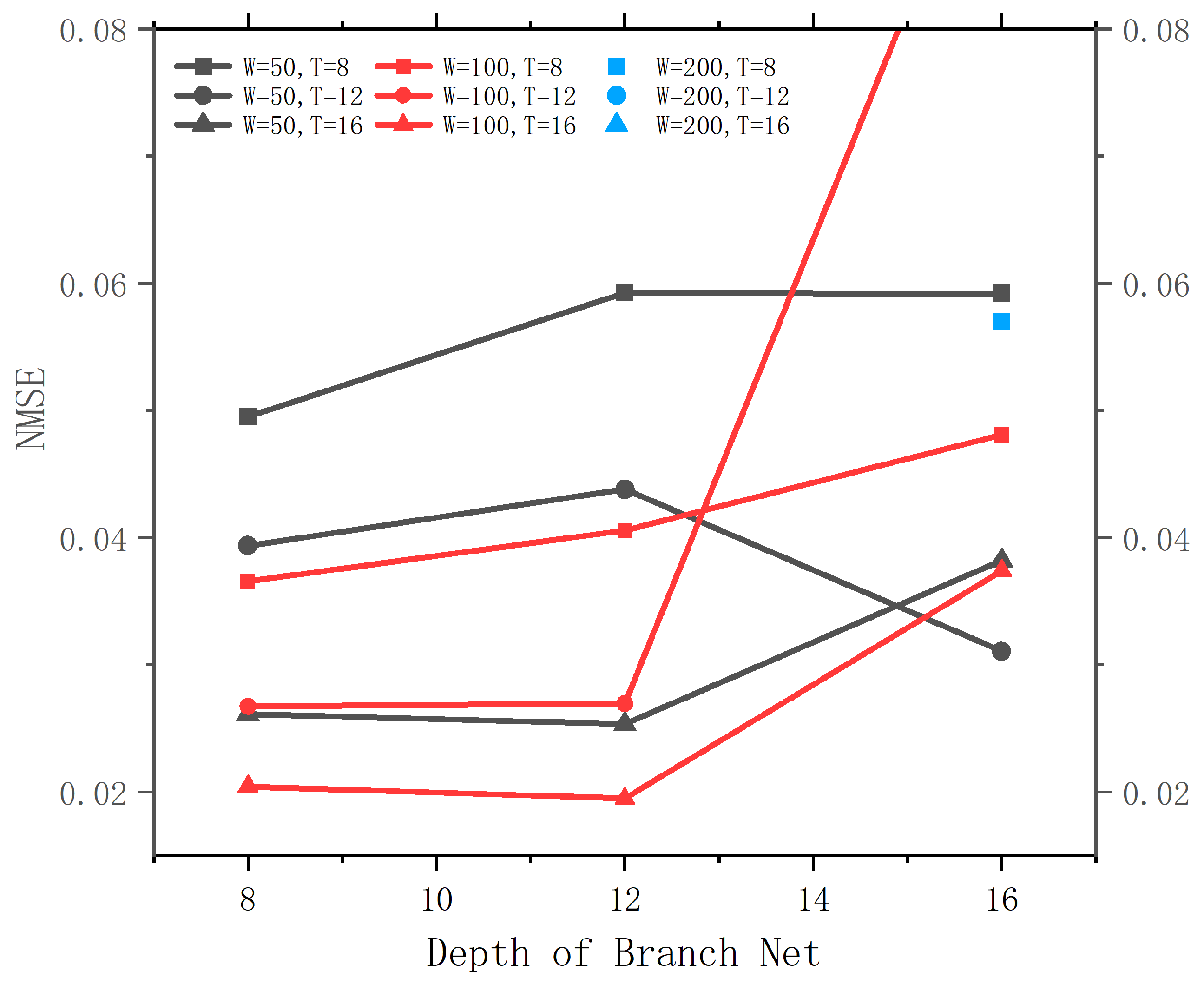
The two sub-networks (branch net and trunk net) are feed-forward networks with constant width (output dimension). Therefore, the width and the depth (the number of fully connected layers) determine the number of parameters, and therefore the capacity of the model. We additionally conducted a hyperparameter search for the model’s width n (We follow the original DeepONet and set the width of the two sub-networks to the same value), the branch net’s depth B, and the trunk net’s depth T. The results are shown in Figure A1. The model displays severe overfitting when the parameters are too large. In the following sections, we used the parameters with the smallest validation NMSE, i.e.,

n = 100

B = 12

T = 16

. This results in 263,701 parameters.

Figure A1. The validation loss of DeepONet using different hidden dimensions and numbers of FNO blocks on the cavity problem.

Appendix B.2. FNN and Other Models in the DeepONet Family

For other models in the DeepONet family and the two FFNs, we generally wish to have their size be similar to other models. We start from the width and depth of the to sub-networks in the DeepONet model, and simply try different widths and depths aroudnd the same magnitude. The hyperparameters concerning the activation functions are the same as in DeepONet.

Appendix B.3. U-Net

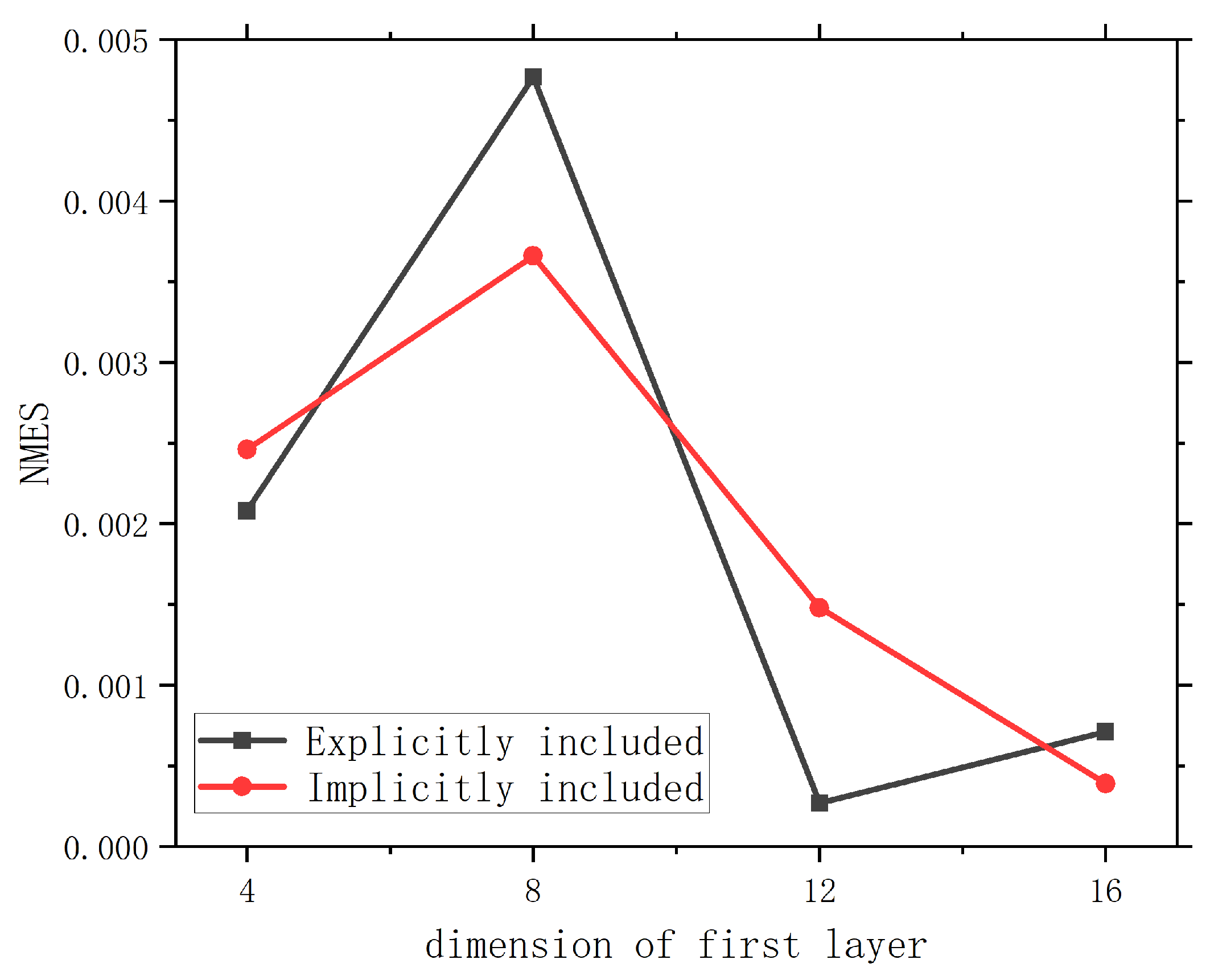
In U-Net, each max-pooling layer is followed by two convolutional layers that double the number of channels. We consider searching the hidden dimension of the first convolutional layer (

d_{2}

) and the means of injecting operating condition parameters

Ω

. We can either explicitly include

Ω

by adding it as addition channels of the input (as described in Section 3.2.3), or we can implicitly include it in the down-sampled hidden representations, i.e., we add a linear layer that projects

Ω

into the same shape as the encoder’s output and add it to that output. When the input explicitly contains

Ω

, its dimensionality (i.e., number of channels) is

d_{1} = 8

, the features are (

u (x, y)

v (x, y)

m a s k

u_{B}, ρ, μ, h, w

) at every location on

(x, y)

, where u and v velocity along the x and y axis. When implicitly conditioning on

Ω

, the input contains only the velocity field. which makes it

d_{1} = 3

, which includes only

u, v

and the mask. For

d_{2}

, it determines the dimensionality of each convolutional layer, thus, the intuition is that the larger

d_{2}

is, the larger the model, and the stronger the learning ability. This is also the trend found by our hyperparameter search. However, a larger model also requires greater computational cost. On the other hand, we observe insignificant differences between the two ways to condition on the operating condition parameters. In the subsequent sections, we explicitly include

Ω

as additional input features (to make it more similar to the FNO structure that we use), and

d_{2} = 12

. This results in 1,095,025 parameters.

Figure A2. The validation loss of U-Net with different hidden dimensions and ways of conditioning on operating parameters on the cavity problem.

Appendix B.4. FNO

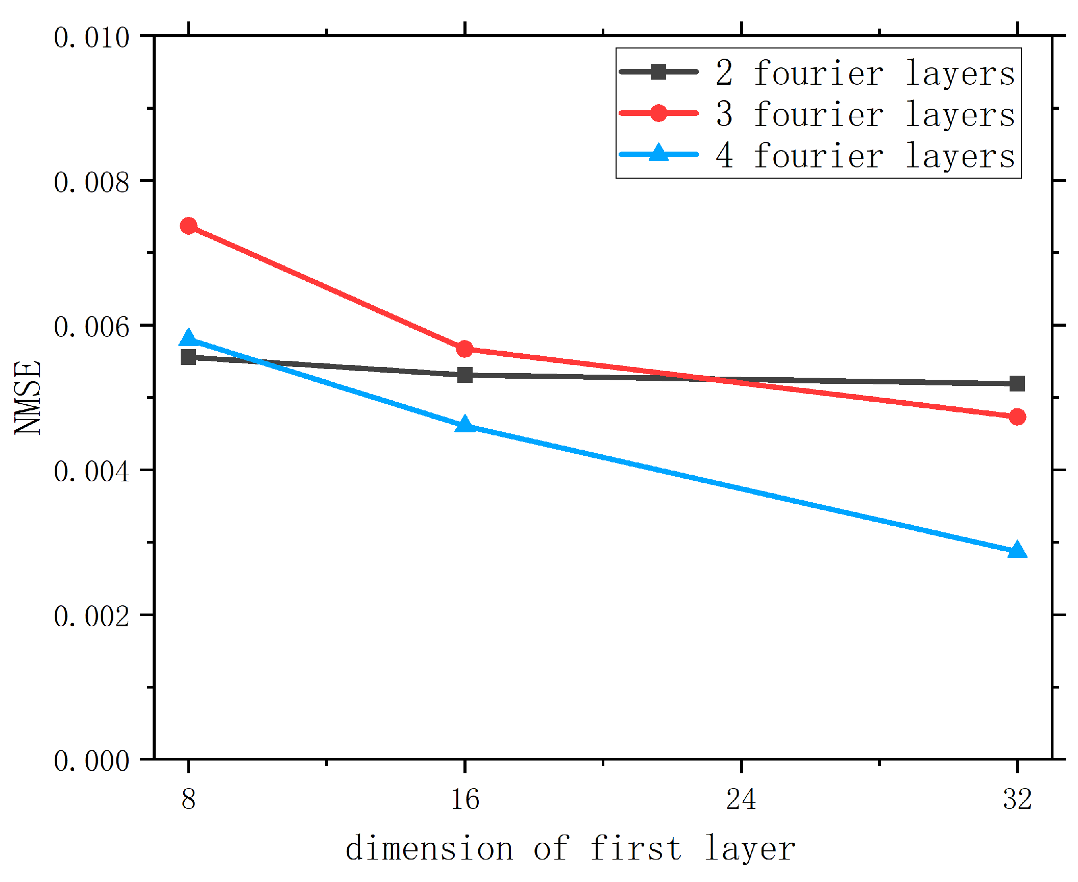
Since the structure of FNO is highly similar to ResNet, we search the same hyperparameters, namely, the number of FNO blocks (d) and the number of channels of the hidden representations (h). We choose to filter out high-frequency signals greater than 12 in the Fourier layer, which is used in the original paper. The results are shown in Figure A3. We observe that increasing both d and h can result in better validation loss, which is intuitive because both imply a greater number of parameters, which increases the capacity of the model. In order to ensure that the number of parameters of the baselines model is similar, such that the training and inference costs are similar, we choose to use

d = 4

and

h = 32

, which results in 1,188,545 parameters.

Figure A3. The validation loss of FNO using different hidden dimensions and number of FNO blocks on the cavity problem.

Appendix C. Data Processing

Appendix C.1. Interpolation Into Grids

Before feeding the data to the neural networks for training, they require some pre-processing. Firstly, all data need to be discretized and interpolated into grids. For simplicity, we also keep the spatial domain to be

64 \times 64

, so for different heights and widths, the size of the grid cells (denoted as

Δ x \times Δ y

) are different. The value of each grid cell is set to be the average of the data points that fall into that cell, and if there is zero data points in a cell, its value is set to be the average of adjacent cells.8

Additionally, for BCs that are constants, we pad the tensor with one extra grid line. For instance, for the tube flow problem, we pad all grids on the top and bottom boundary with one line of zeros, resulting in a tensor with 66 rows and 64 columns.

References

Lodhi Devendra, K.A. Dam-break flood simulation under various likely scenarios and mapping using gis: Case of a proposed dam on river yamuna, india. J. Mt. Sci. 2012, 9, 214–220. [Google Scholar] [CrossRef]
Aidun, C.K.; Triantafillopoulos, N.G.; Benson, J.D. Global stability of a lid-driven cavity with throughflow: Flow visualization studies. Phys. Fluids 1991, 3, 2081–2091. [Google Scholar] [CrossRef]
Bi, K.; Xie, L.; Zhang, H.; Chen, X.; Gu, X.; Tian, Q. Accurate medium-range global weather forecasting with 3d neural networks. Nature 2023, 619, 533–538. [Google Scholar] [CrossRef] [PubMed]
Brown, T.B.; Mann, B.; Ryder, N.; Subbiah, M.; Kaplan, J.; Dhariwal, P.; Neelakantan, A.; Shyam, P.; Sastry, G.; Askell, A.; et al. Language models are few-shot learners. arXiv 2020, arXiv:abs/2005.14165. [Google Scholar]
Cao, Q.; Goswami, S.; Karniadakis, G.E. Lno: Laplace neural operator for solving differential equations. arXiv 2023, arXiv:2303.105283. [Google Scholar]
Chen; Shiyi; Doolen; Gary, D. Lattice boltzmann method for fluid flows. Annu. Rev. Fluid Mech. 1998. [Google Scholar] [CrossRef]
Chiu, Pa.; Wong, J.; Ooi, C.; Dao, M.; Ong, Y. Can-pinn: A fast physics-informed neural network based on coupled-automatic-numerical differentiation method. 2021.
Jacob Devlin, Ming-Wei Chang, Kenton Lee, and Kristina Toutanova. Bert: Pre-training of deep bidirectional transformers for language understanding. arXiv 2019, arXiv:abs/1810.04805.
Stefan Elfwing, Eiji Uchibe, and Kenji Doya. Sigmoid-weighted linear units for neural network function approximation in reinforcement learning. 2017.
Alexandre Ern and Jean-Luc Guermond. Theory and Practice of Finite Elements; Springer: Berlin/Heidelberg, Germany, 2004; Volume 159. [Google Scholar]
Frutos, D.; Javier, N. A spectral element method for the navier-stokes equations with improved accuracy. Siam J. Numer. Anal. 2000. [Google Scholar] [CrossRef]
Fukushima, K. Neocognitron: A self-organizing neural network model for a mechanism of pattern recognition unaffected by shift in position. Biol. Cybern. 1980, 36, 193–202. [Google Scholar] [CrossRef]
Gao, H.; Sun, L.; Wang, Ji. Phygeonet: Physics-informed geometry-adaptive convolutional neural networks for solving parameterized steady-state pdes on irregular domain. J. Comput. Phys. 2021, 428, 110079. [Google Scholar] [CrossRef]
Ghia, U.; Ghia, K.N.; Shin, C.T. High-re solutions for incompressible flow using the navier-stokes equations and a multigrid method. J. Comput. Phys. 1982, 48, 387–411. [Google Scholar] [CrossRef]
Goodfellow, I.J.; Pouget-Abadie, J.; Mirza, M.; Xu, B.; Warde-Farley, D.; Ozair, S.; Courville, A.C.; Bengio, Y. Generative adversarial nets; NIPS: 2014.
Hadorn, P.S. Shift-deeponet: Extending deep operator networks for discontinuous output functions. 2022.
He, K.; Zhang, X.; Ren, S.; Sun, J. Delving deep into rectifiers: Surpassing human-level performance on imagenet classification. 2015 IEEE International Conference on Computer Vision (ICCV), 1026. [Google Scholar]
He, K.; Zhang, X.; Ren, S.; Sun, J. Deep residual learning for image recognition. IEEE: 2016.
Hochreiter, S.; Schmidhuber, J. Long short-term memory. Neural Comput. 1997, 9, 1735–1780. [Google Scholar] [CrossRef] [PubMed]
Kurt Hornik, Maxwell Stinchcombe, and Halbert White. Multilayer feedforward networks are universal approximators. Neural Netw.s 1989, 2, 359–366. [Google Scholar] [CrossRef]
Hu, Z.; Jagtap, A.D.; Karniadakis, G.E.; Kawaguchi, K. Augmented physics-informed neural networks (apinns): A gating network-based soft domain decomposition methodology. arXiv 2022, arXiv:2211.08939. [Google Scholar] [CrossRef]
Huang, Z.; Schneider, T.; Li, M.; Jiang, C.; Zorin, D.; Panozzo, D. A large-scale benchmark for the incompressible navier-stokes equations. 2021.
Isola, P.; Zhu, Ju.; Zhou, T.; Efros, A.A. Image-to-image translation with conditional adversarial networks. In 2017 IEEE Conference on Computer Vision and Pattern Recognition (CVPR), 2017.
Jagtap, A.D.; Karniadakis, G.E. Extended physics-informed neural networks (xpinns): A generalized space-time domain decomposition based deep learning framework for nonlinear partial differential equations. In AAAI spring symposium: MLPS, volume 10, 2021.
Jagtap, A.D.; Kharazmi, E.; Karniadakis, G.E. Conservative physics-informed neural networks on discrete domains for conservation laws: Applications to forward and inverse problems. Comput. Methods Appl. Mech. Eng. 2020, 365, 113028. [Google Scholar] [CrossRef]
Kochkov, D.; Smith, J.; Alieva, A.; Wang, Q.; Brenner, M.; Hoyer, S. Machine learning accelerated computational fluid dynamics. 2021.
Kovachki, N.B.; Li, Z.; Liu, B.; Azizzadenesheli, K.; Bhattacharya, K.; Stuart, A.M.; Anandkumar, A. Neural operator: Learning maps between function spaces. CoRR, 2108. [Google Scholar]
Yann LeCun, Y. Bengio, and Geoffrey Hinton. Deep learning. Nature 2015, 521, 436–44. [Google Scholar]
Li, Z.; Kovachki, N.; Azizzadenesheli, K.; Liu, B.; Bhattacharya, K.; Stuart, A.; Anandkumar, A. Fourier neural operator for parametric partial differential equations, 2020.
Li, Z.; Zheng, H.; Kovachki, N.; Jin, D.; Chen, H.; Liu, B.; Azizzadenesheli, K.; Anandkumar, A. Physics-informed neural operator for learning partial differential equations. arXiv 2021, arXiv:2111.03794. [Google Scholar]
Lin, G.; Moya, C.; Zhang, Z. B-deeponet: An enhanced bayesian deeponet for solving noisy parametric pdes using accelerated replica exchange sgld. J. Comput. Phys. 2023, 473, 111713. [Google Scholar] [CrossRef]
Lu, L.; Jin, P.; Pang, G.; Zhang, Z.; Karniadakis, G.E. Learning nonlinear operators via deeponet based on the universal approximation theorem of operators. Nat. Mach. Intell. 2019, 3, 218–229. [Google Scholar] [CrossRef]
Lu, L.; Meng, X.; Cai, S.; Mao, Z.; Goswami, S.; Zhang, Z.; Karniadakis, G.E. A comprehensive and fair comparison of two neural operators (with practical extensions) based on fair data. Comput. Methods Appl. Mech. Eng. 2022, 393, 114778. [Google Scholar] [CrossRef]
Oldenburg, J.; Borowski, F.; Öner, A.; Schmitz, Kl.; Stiehm, M. Geometry aware physics informed neural network surrogate for solving navier–stokes equation (gapinn). Adv. Model. Simul. Eng. Sci. 2022, 9, 8. [Google Scholar] [CrossRef]
Quiroga, V.M. 2d dam break flood simulation with hec-ras: Chepete dam. 2021.
Raissi, M.; Perdikaris, P.; Karniadakis, G.E. Physics-informed neural networks: A deep learning framework for solving forward and inverse problems involving nonlinear partial differential equations. J. Comput. Phys. 2019, 378, 686–707. [Google Scholar] [CrossRef]
Ren, P.; Rao, C.; Liu, Y.; Wang, Ji.; Sun, H. Phycrnet: Physics-informed convolutional-recurrent network for solving spatiotemporal pdes. Computer Methods in Applied Mechanics and Engineering, Computer Methods in Applied Mechanics and Engineering.
Ritz, W. Über eine neue methode zur lösung gewisser variationsprobleme der mathematischen physik. 1909.
Rombach, R.; Blattmann, A.; Lorenz, D.; Esser, P.; Ommer, B. High-resolution image synthesis with latent diffusion models. 2022 IEEE/CVF Conference on Computer Vision and Pattern Recognition (CVPR), 1067. [Google Scholar]
Ronneberger, O.; Fischer, P.; Brox, T. U-net: Convolutional networks for biomedical image segmentation. CoRR, 1505. [Google Scholar]
Schlicting, H. Boundary layer theory; Mcgraw-hill: 1960.
Shankar, P.N.; Deshpande, M.D. Fluid mechanics in the driven cavity. Annu. Rev. Fluid Mech. 2000, 32, 93–136. [Google Scholar] [CrossRef]
Sønderby, C.K.; Espeholt, L.; Heek, J.; Dehghani, M.; Oliver, A.; Salimans, T.; Hickey, J.; Agrawal, S.; Kalchbrenner, N. Metnet: A neural weather model for precipitation forecasting. Submiss. J. 2020. [Google Scholar]
Allen Taflove. Computational electrodynamics the finite-difference time-domain method. 1995.
Takamoto, M.; Praditia, T.; Leiteritz, R.; MacKinlay, D.; Alesiani, F.; Pflüger, D.; Niepert, M. Pdebench: An extensive benchmark for scientific machine learning. Advances in Neural Information Processing Systems 2022, 35, 1596–1611. [Google Scholar]
Tan, L.; Chen, L. Enhanced deeponet for modeling partial differential operators considering multiple input functions. 2022.
Venturi, S.; Casey, T. Svd perspectives for augmenting deeponet flexibility and interpretability. Comput. Methods Appl. Mech. Eng. 2023, 403, 115718. [Google Scholar] [CrossRef]
Versteeg, H.K.; Malalasekera, W. An introduction to computational fluid dynamics - the finite volume method. 2007.
Wang, S.; Wang, H.; Perdikaris, P. Improved architectures and training algorithms for deep operator networks, 2021.
Wang, S.; Wang, H.; Perdikaris, P. Learning the solution operator of parametric partial differential equations with physics-informed deeponets. Sci. Adv. 2021, 7. [Google Scholar] [CrossRef]
Xiong, W.; Huang, X.; Zhang, Z.; Deng, R.; Sun, P.; Tian, Y. Koopman neural operator as a mesh-free solver of non-linear partial differential equations. arXiv 2023, arXiv:2301.10022. [Google Scholar]
Xu, W.; Lu, Y.; Wang, L. Transfer learning enhanced deeponet for long-time prediction of evolution equations. 2022.
Zhu, Ju.; Park, T.; Isola, P.; Efros, A.A. Unpaired image-to-image translation using cycle-consistent adversarial networks. In 2017 IEEE International Conference on Computer Vision (ICCV), Oct 2017.
Zienkiewicz, O.C.; Taylor, R.L.; Zhu, J.Z.; Bl, E.; Hhintalann, T. The finite element method. 1977.

1	In this paper, we regard all models that accept a query location, and have an independent network (i.e., the trunk net) for encoding query locations, and predict values at those locations. However, the differences between the DeepONet family and image-to-image models are subtle, and may be viewed as some variants of one another.
2	Interestingly, a ResNet block adds the input to the output of a CNN block, which is $x + f (x)$ and is similar to many iterative numerical methods.
3	$f \circ g$ denotes the composite of f and g.
4	Preliminary experiments show that using a different loss function for training (e.g., using MSE instead of NMSE) does not impact the primary conclusions about the behaviors of the models that are drawn from the results. The only significant behavior change is that the loss function used for training will be smaller on the test data. Thus, this work only train the baseline models using NMSE.
5	An alternative for fair comparison is to align the computational cost (for training and testing) of the models, which is another important practical concern in the application of CFD modeling methods.
6	We regard situations where the prediction is worse than the identity transformation as failure to converge.
7	Efficicent in terms of inference speed, compared with autoregressive models of roughly the same size.
8	For multiple contiguous empty cells, we set their value iteratively from the boundaries of the empty region.

Figure 1. Some examples of the velocity field in the four problems in CFDBench. From left to right: cavity flow, tube flow, dam flow, and cylinder flow.

Figure 2. The residuals of each flow problems in this paper. (a) cavity flow, (b) tube flow, (c) dam flow, (d) cylinder flow.

Figure 3. Overview of the input and output types and shapes of each baseline model.

Figure 4. The structure of each baseline model in this paper.

Figure 5. Prediction of the velocity field by the baseline models on the cavity and tube flow problems. The result of autoregressive models is the prediction of one forward propagation step. The input is not given to non-autoregressive models.

Figure 6. Prediction of the velocity field by the baseline models on the dam and cylinder flow problems. The result of autoregressive models is the prediction of one forward propagation step. The input is not given to non-autoregressive models.

Figure 7. Summary of the performance of autoregressive baseline methods on the four problems (with all cases). FNO’s result on the dam flow problem is removed because the error is too large and including it would make the plot less intelligible. The bar chart of the cylinder flow (d) is in logarithmic scale.

Figure 8. The error of autoregressive and non-autoregressive baselines as a function of the number of forward propagation steps, given only the operating parameters

Ω

and the initial conditions. The y-axis is on a logarithmic scale. ResNet is not included because its error is too high and including its line would make the figure less intelligible. Best viewed in color.

Figure 8. The error of autoregressive and non-autoregressive baselines as a function of the number of forward propagation steps, given only the operating parameters

Ω

Table 5. Breakdown of the number of cases in each problem (the rows) and the corresponding subsets (the columns) in CFDBench. Each problem contains three subsets, each with one type of operating condition parameter that is varied.

	Number of cases					Each frame
Problem	BC	PROP	GEO	Total	# frames	File Size	Gen. Time
Cavity Flow	50	84	25	159	34,582	5.2 MB	0.92s
Tube Flow	50	100	25	175	39,553	4.8 MB	1.08s
Dam Flow	70	100	50	220	21,916	2.0 MB	3.98s
Cylinder Flow	50	115	20	185	205,620	4.4 MB	1.18s
Sum	220	399	120	739	301,671

Table 6. Overview of the different baseline models we consider. “Auto.” refers to whether the method is autoregressive.

u_{sample}

is a list of samples points from u.

Table 6. Overview of the different baseline models we consider. “Auto.” refers to whether the method is autoregressive.

u_{sample}

is a list of samples points from u.

Method	Auto.	Inp. Shape	Outp. Shape	Inputs	Outputs
FFN	No	Any	Any	$(x, y, t), Ω$	$\hat{u} (x, y, t)$
DeepONet	No	Any	Any	$(x, y, t), Ω$	$\hat{u} (x, y, t)$
Auto-FFN	Yes	Any	Any	$u_{sample} (t - Δ t), Ω, (x, y)$	$\hat{u} (x, y, t)$
Auto-DeepONet	Yes	Any	Any	$u_{sample} (t - Δ t), Ω, (x, y)$	$\hat{u} (x, y, t)$
Auto-EDeepONet	Yes	Any	Any	$u_{sample} (t - Δ t), Ω, (x, y)$	$\hat{u} (x, y, t)$
Auto-DeepONetCNN	Yes	Grid	Any	$u (t - Δ t), Ω, (x, y)$	$\hat{u} (x, y, t)$
ResNet	Yes	Grid	Grid	$u (t - Δ t), Ω$	$\hat{u} (t)$
U-Net	Yes	Grid	Grid	$u (t - Δ t), Ω$	$\hat{u} (t)$
FNO	Yes	Grid	Grid	$u (t - Δ t), Ω$	$\hat{u} (t)$

Table 7. The validation loss of ResNet and the identity transformation for the 7 subsets (see Section 5) in the cavity flow problem. The better result is highlighted in bold.

Method	(1)	(2)	(3)	(4)	(5)	(6)	(7)
NMSE
Identity	0.100	0.108	0.076	0.108	0.097	0.112	0.111
ResNet	0.065	0.147	0.863	0.200	0.094	0.156	0.080
MSE
Identity	0.343	0.031	0.029	0.149	0.028	0.347	0.164
ResNet	0.065	0.044	0.500	0.119	0.027	0.339	0.058
MAE
Identity	0.166	0.076	0.057	0.120	0.067	0.167	0.119
ResNet	0.112	0.146	0.624	0.166	0.098	0.296	0.130

Table 8. Main test results of non-autoregressive methods (FFN and DeepONet) on each subset of each problem.

Problem	Subset	NMSE		MSE		MAE
		FFN	DeepONet	FFN	DeepONet	FFN	DeepONet
Cavity	(1) PROP	0.0099592	0.0291865	0.0473762	0.1693782	0.1111506	0.5680576
	(2) BC	0.0023445	0.1110036	0.2437581	13.2787848	0.2882956	1.7553163
	(3) Geo	0.6239881	0.5806319	1.8697622	1.9919338	0.9227801	0.9277460
	(4) PROP + BC	0.0084082	0.0799971	0.2003079	3.3371139	0.2580179	0.8954092
	(5) PROP + GEO	0.1242569	0.0892609	0.3536154	0.3205143	0.2056559	0.2610952
	(6) BC + GEO	0.1161350	0.2098982	1.1426576	10.0195319	0.5412614	1.5829833
	(7) All	0.0221644	0.0646872	0.7857684	4.0079125	0.4356092	1.0548950
Tube	(1) PROP	0.0004197	0.0039994	0.0002522	0.0026946	0.0078708	0.0315951
	(2) BC	19.2247428	25.8505255	1.4869019	1.3689488	0.7780905	0.7297134
	(3) GEO	0.1674582	0.1861845	0.1735853	0.1708268	0.2698841	0.3242756
	(4) PROP + BC	3.7321264	5.8203221	0.5254855	0.4897547	0.3910940	0.3403379
	(5) PROP + GEO	0.6573232	0.5961287	0.1125305	0.1187899	0.1520187	0.1924667
	(6) BC + GEO	0.6412595	0.5119403	1.7430317	2.1646790	0.8040325	0.8678228
	(7) All	3.0935680	0.3437079	0.5307588	0.4553377	0.3303886	0.3416610
Dam	(1) PROP	0.0004000	0.0205820	0.0002025	0.0104605	0.0080647	0.0602617
	(2) BC	0.3882083	0.0145171	0.1656223	0.0098575	0.2962269	0.0512015
	(3) GEO	0.0408200	0.0438950	0.0101389	0.0109773	0.0449910	0.0517545
	(4) PROP + BC	0.3830672	0.0048370	0.0522189	0.0019914	0.1178206	0.0223580
	(5) PROP + GEO	0.0190430	0.0567282	0.0060118	0.0231003	0.0319056	0.0772180
	(6) BC + GEO	0.0982004	0.3650784	0.0431119	0.1924977	0.1442159	0.3337956
	(7) All	0.1694195	0.0686736	0.0705092	0.0270029	0.1362603	0.1007961
Cylinder	(1) PROP	0.0007879	0.0021776	0.0008786	0.0024212	0.0141193	0.0254937
	(2) BC	0.0108285	9.7361195	0.0682347	4.0023353	0.1358656	1.5573399
	(3) GEO	0.1405526	108.5875535	0.1648840	119.6764528	0.2541922	5.7167007
	(4) PROP + BC	0.8656293	0.2141155	0.9652876	0.4134728	0.2702630	0.4543390
	(5) PROP + GEO	0.0249946	0.1252280	0.0290181	0.1412260	0.0731633	0.2759877
	(6) BC + GEO	0.0560368	0.0570367	0.0899771	0.0966049	0.1741357	0.1707578
	(7) All	0.0281058	2.3627123	0.0472888	3.0325988	0.1155052	1.2104118

Table 9. Computational cost of the different baseline models on the cavity flow data, PROP subset. training time refers to the time required for training before using the model, inference time refers to the time required for computing one forward propagation (for autoregressive models) or the prediction on one query point (for non-autoregressive models).

		Training		Inference
Method	# Param.	Time (min)	Mem. (MB)	Time (ms)	Mem. (MB)
Non-Autoregressive Models
FFN	72K	30	443	6.4	7.2
DeepONet	143K	28	355.1	7.2	10.3
Autoregressive Models
Auto-FFN	1,102K	313	4,127	7.5	135.9
Auto-DeepONet	552K	15	151	6.0	5.6
Auto-EDeepONet	623K	16	153	6.0	5.9
Auto-DeepONetCNN	743K	100	1,367	10.3	38.9
ResNet	522K	105	1,073	10.5	5.5
FNO	1,189K	43	475	9.7	13.6
U-Net	1,095K	33	224	11.0	46.1

Disclaimer/Publisher’s Note: The statements, opinions and data contained in all publications are solely those of the individual author(s) and contributor(s) and not of MDPI and/or the editor(s). MDPI and/or the editor(s) disclaim responsibility for any injury to people or property resulting from any ideas, methods, instructions or products referred to in the content.

© 2023 by the authors. Licensee MDPI, Basel, Switzerland. This article is an open access article distributed under the terms and conditions of the Creative Commons Attribution (CC BY) license (http://creativecommons.org/licenses/by/4.0/).

Copyright: This open access article is published under a Creative Commons CC BY 4.0 license, which permit the free download, distribution, and reuse, provided that the author and preprint are cited in any reuse.

MDPI Initiatives

Important Links

Choose an area of interest and we will send you notifications of new preprints at your preferred frequency.

Disclaimer

CFDBench: A Comprehensive Benchmark for Machine Learning Methods in Fluid Dynamics

Abstract

1. Introduction

2. Related Works

Numerical Methods

Neural Networks

Neural Operators for Solving PDEs

3. CFDBench

3.1. The Definition of Flow Problems

3.2. Cavity Flow

3.3. Tube Flow

3.4. Dam Flow

3.5. Cylinder Flow

3.6. Data Generation

3.6.1. Data Splitting

4. Experiments

4.1. Training Objectives

Non-Autoregressive Modeling

Autoregressive Modeling

4.2. Baselines

4.3. Non-Autoregressive Baselines

4.3.1. FNN

4.3.2. DeepONet

4.4. Autoregressive Baselines

4.4.1. Autoregressive FFN

4.4.2. Autoregressive DeepONet

4.4.3. Autoregressive EDeepONet

4.4.4. Autoregressive DeepONetCNN

4.4.5. ResNet

4.4.6. U-Net

4.4.7. FNO

4.5. Conditioning on Operating Parameters

4.6. Loss Functions

Mean Square Error (MSE)

Normalized Mean Square Error (NMSE)

Mean Absolute Error (MAE)

4.7. Hyperparameter Search

4.7.1. ResNet

4.8. Other Details

5. Results

5.1. Single Step Prediction

5.1.1. Non-Autoregressive Modeling

5.1.2. Autoregressive Modeling

5.2. Multi-Step Prediction

5.3. Computational Cost

6. Conclusions

Data Availability Statement

Appendix A. Mathematical Notations

Appendix B. Hyperparameters of Baseline Neural Networks

Appendix B.1. DeepONet

Appendix B.2. FNN and Other Models in the DeepONet Family

Appendix B.3. U-Net

Appendix B.4. FNO

Appendix C. Data Processing

Appendix C.1. Interpolation Into Grids

References

MDPI Initiatives

Important Links

Subscribe