Preprint

Article

Short-Term Photovoltaic Power Forecasting Based on a Feature Rise-Dimensional Two-Layer Ensemble Learning Model

Altmetrics

Downloads

107

Views

Comments

A peer-reviewed article of this preprint also exists.

This version is not peer-reviewed

Submitted:

21 September 2023

Posted:

22 September 2023

You are already at the latest version

Alerts

Abstract

Due to the intermittency and fluctuation of photovoltaic (PV) output power, a high proportion of grid-connected PV power generation systems has a significant impact on power systems. Accurate PV power forecasting can alleviate the uncertainty of the PV power and is of great significance for the stable operation and scheduling of the power systems. Therefore, in this study, a feature rise-dimensional (FRD) two-layer ensemble learning (TLEL) model for short-term PV power deterministic forecasting and probability forecasting is proposed. First， based on the eXtreme Gradient Boosting (XGBoost), Random Forest (RF), CatBoost, and Long-short-term memory (LSTM) models, a TLEL model is constructed utilizing the ensemble learning algorithm. Meanwhile, the FRD method is introduced to construct the FRD-XGBoost-LSTM (R-XGBL), FRD-RF-LSTM(R-RFL), and FRD- CatBoost - LSTM (R-CatBL) models. Subsequently, the above models are combined to construct the FRD-TLEL model for deterministic forecasting, and perform probability interval forecasting based on quantile regression(QR). Finally, the performance of the proposed model is demonstrated with a real-world dataset. By comparing with other models, the proposed model displays better forecasting accuracy for deterministic forecasting and reliable forecasting intervals for probability forecasting, and good generalization ability in the datasets of different seasons and weather types.

Keywords:

Subject: Computer Science and Mathematics - Artificial Intelligence and Machine Learning

1. Introduction

In recent years, under the influence of multiple factors such as climate change, energy security, economic development, and technological progress, countries around the world have increased their exploration and development of green new energy, and the energy structure has gradually transitioned towards "clean" and "low-carbon". As a renewable energy source, solar energy has been widely and intensively applied due to its strong renewable ability, clean environmental protection, abundant resources, and convenient development and utilization [1,2]. The proportion of photovoltaic (PV) power generation in the power system is increasing year by year. According to the data from the International Energy Agency, by 2027, installed PV power capacity will surpass that of coal and become the world's largest. However, due to the significant impact of meteorological and other factors on the PV power output, which has strong intermittency and volatility, these characteristics make high-proportion grid-connected PV power systems a huge impact and challenge to the power system [3]. If the PV power output can be accurately forecasted, it can not only improve the utilization rate of renewable energy but also help the scheduling department adjust the scheduling plan to ensure the safe and stable operation of the power system after a high proportion of PV connections [4].

PV power forecasting methods can be classified into medium-, long-term power forecasting, short-term power forecasting, and ultra-short-term power forecasting based on different forecasting time scales [5]. Medium- and long-term power forecasting can forecast the PV power from 1 month to 1 year. The required accuracy is not high, and it is mainly used for services such as site selection, design, and consulting of PV power plants [6]. Short-term PV power forecasting can predict the PV power in the next 1-3 days, and the results are mainly utilized by the dispatch department to formulate a daily power generation plan [7]. Ultra-short-term PV power forecasting mainly predicts the PV power output within the next 15 minutes to 4 hours, and the results are mainly used as a reference for real-time scheduling of the power grid [8]. From the perspective of different modeling methods, PV power forecasting can be classified into physical methods and statistical methods [9]. Physical methods are based on the use of precise instruments to measure meteorological factors such as solar irradiance and temperature, and various intelligent algorithms or complex formulas are utilized to derive calculations for forecasting, which are rarely used in practical production [10]. The statistical method mainly involves statistical analysis of the historical data on meteorological factors, as well as the PV output power, to identify the relationship between them and establish a PV power forecasting model [11]. From the perspective of different forecasting algorithms, PV power forecasting can be classified into linear forecasting, nonlinear forecasting, and combination forecasting algorithms [12]. Linear forecasting includes time series analysis, linear regression, autoregressive integral moving average (ARIMA) algorithm, etc. Nonlinear forecasting includes Markov chain, support vector machine(SVM), neural network, wavelet analysis, random forest (RF), deep learning (DL) algorithms, etc. [13]. Rafati et al. [14] presented a univariate data-driven method to improve the accuracy of very short-term solar power forecasting. The feasibility of the proposed method is verified by comparing the forecasting results with neural networks, support vector regression, and RF algorithms. In the literature [15], a SVM was constructed based on the processed data. The improved ant colony algorithm was used to optimize the parameters of the SVM, which significantly improved the forecasting accuracy of peak power and nighttime power.

However, using a single forecasting model for forecasting has limitations and often cannot achieve satisfactory forecasting results. Many scholars consider combining different algorithms. Huang et al. [16] developed a new time series forecasting based on an algorithm that combines conditional generative adversarial networks with convolutional neural networks (CNN) and Bi-directional long short-term memory (Bi-LSTM) to improve the accuracy of hourly PV power forecasting. Compared with long-short-term memory (LSTM), recurrent neural network (RNN), backpropagation neural network (BP), SVM, and Persistence models, the proposed model has been verified to have better performance in forecasting accuracy. Banik and Biswas [17] designed a solar irradiance and PV power output model using a combination of RF and CatBoost algorithms, and then conducted long-term monthly prediction using 10 years of solar data and other relevant meteorological parameters with a sampling interval of 1 hour to verify the feasibility and applicability of the proposed model. In [18], a day-ahead PV power forecasting model that fuses DL modeling and time correlation principles was proposed. Firstly, an independent day-ahead PV power forecasting model based on LSTM -RNN was established, and then the model was modified based on the principle of time correlation. Guo et al. [19] employed a PV power forecasting model based on stacking ensemble learning algorithms. The operational state parameters and meteorological parameters of PV panels were utilized to iteratively train the single model and the stacking model. The eXtreme Gradient Boosting (XGBoost) algorithm was selected to compare with the Stacking algorithm to verify the superiority of the proposed model.

The above combination models combine different single PV forecasting models to achieve complementary advantages and further improve the accuracy of PV power forecasting. However, during data processing, some features are filtered out from the original data through some methods and directly used as input to the model. These methods, which can be called feature dimensionality reduction, improve the computational efficiency of the model but weaken the initial features. In addition, errors are inevitable during the training process, so there is still room for improvement in the accuracy of the forecasting results.

According to different forms of forecasting results, PV power forecasting can be classified into two main categories: deterministic forecasting and probabilistic forecasting. The output of the deterministic forecasting model is only the PV power output results at certain time points [20,21,22], which cannot evaluate the uncertainty in PV power generation data. Probability forecasting can be divided into probability interval forecasting [23,24] and probability density forecasting methods [24]. Probability density forecasting can determine the possible values and probabilities of photovoltaic power output based on the cumulative probability distribution function or probability density function, including parametric methods [25] and non-parametric methods [26]. Probability interval forecasting can obtain the forecasting fluctuation range of PV power output, thereby providing an accurate PV power variation range for scheduling plans to assist in scheduling decisions [26]. In the literature [27], the natural gradient boosting algorithm was selected to generate PV power probability forecasting results with different confidence intervals. In the literature [28], firstly, the fuzzy c-means (FCM) clustering algorithm was used to cluster the numerical weather forecast and historical data of PV power plants. The white optimization algorithm (WOA) was employed for optimizing the penalty factor and kernel width of the least squares support vector machine (LSSVM) model. Then, the clustering numerical weather forecast and historical data of PV power plants were utilized to train the WOA-LSSVM forecasting model to predict the future day's PV power output. The density distribution of forecasting error was obtained to generate different confidence intervals. Long et al. [29] proposed a combined interval forecasting model based on upper and lower bound estimation to quantify the uncertainty of solar energy prediction. In the proposed model, the boundary was predicted separately by two forecasting engines. Using extreme learning machine (ELM) as the basic forecasting engine and automatic encoder technology to initialize the input weight matrix for effective feature learning. A novel biased convex cost function was developed for ELM to predict the interval boundary. The convex optimization technique was used to process the output weight matrix of ELM. Pan et al. [30] proposed a range forecasting method for solar power generation based on a gated recursive unit (GRU) neural network and kernel density estimation (KDE). The deterministic forecasting results of solar power generation were acquired using GRU with an attention mechanism. The error of the deterministic forecasting results was fitted using the KDE method, and the probability density function and cumulative distribution function of solar power error at different time periods were achieved. Furthermore, a confidence interval of 90% for solar power output forecasting was obtained.

Compared with deterministic forecasting, probabilistic forecasting can better evaluate the uncertainty of PV power output. However, to our knowledge, its research is relatively insufficient, and further research is still needed.

Therefore, the objective of this study is to propose a feature rise-dimensional(FRD) two-layer ensemble learning (TLEL) model for short-term PV power deterministic forecasting and probability interval forecasting to improve forecasting accuracy. More specifically, the raw data is first cleaned and correlation analysis is conducted between PV power output and various meteorological features. In addition, weather category construction is performed by the K-means clustering algorithm on meteorological data lacking meteorological category classification. Then, based on the XGBoost, RF, CatBoost, and LSTM models, a TLEL model is constructed using an ensemble learning algorithm. Concurrently, feature engineering is introduced to perform FRD optimization on it. After that, the FRD-XGBoost- LSTM(R-XGBL), FRD-RF- LSTM(R-RFL), FRD-CatBoost - LSTM (R-CatBL), and TLEL models are combined using the reciprocal error method to construct the FRD-TLEL Model for the deterministic forecast. Next, the probability interval forecasting model based on quantile regression(QR) considering deterministic forecasting results is constructed. Finally, based on the data from different seasons and weather types, the effectiveness and superiority of the proposed forecasting model are verified by comparing it with other models.

The main contributions of the research are summarized as follows:

Considering the limitations of a single forecasting model, based on the XGBoost, RF, CatBoost, and LSTM models, combined with the ensemble learning framework pattern, a new short-term PV power deterministic forecasting model based on TLEL is proposed. This model can weaken the problem of poor data authenticity and coherence caused by rough data preprocessing to improve forecasting accuracy.
Considering that feature dimensionality reduction during data preprocessing weakens initial features, the FRD method utilized to optimize forecasting datasets is proposed, which enables the model to carry more original data features based on ensemble learning. In the proposed FRD-TLEL model, the forecasting results of the TLEL model and each model optimized by the FRD method are weighted by the reciprocal error method to obtain the final forecasting results, which effectively improves the forecasting accuracy.
The FRD-TLEL model has good generalization ability and is suitable for deterministic forecasting and probability forecasting in the datasets of different seasons and weather types.

The remainder of this paper is organized as follows: The data sources, data preprocessing, and forecasting methods are given in Section 2; the forecasting results, comparison, and discussion are presented in Section 3; Section 4 elaborates on the conclusions and further research suggestions.

2. Methodology

2.1 Framework for Proposed Methods

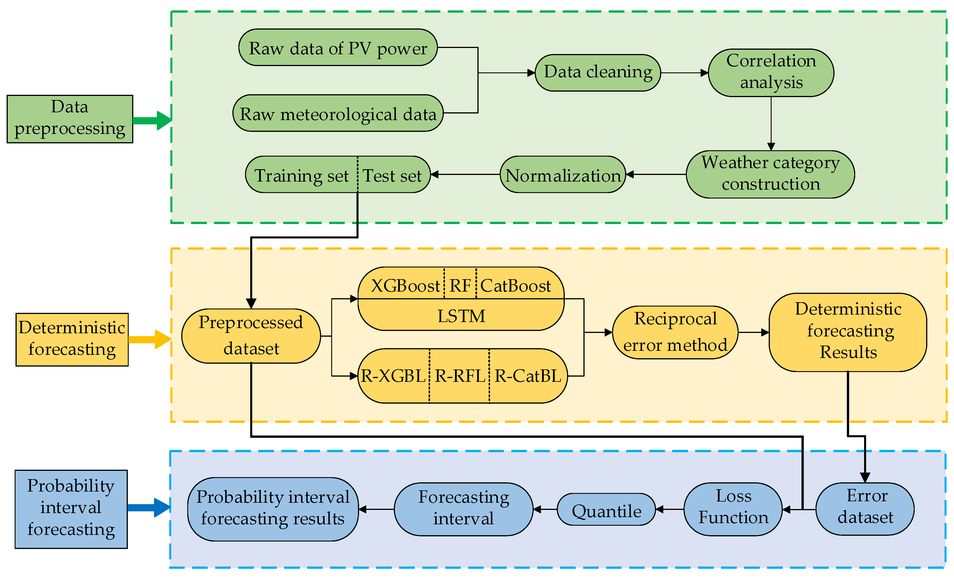
The overall framework of the PV power forecasting in this paper is shown in Figure 1, which mainly consists of three modules.

Data preprocessing. First, the raw PV power output data and meteorological data are cleaned. Next, the meteorological features are selected by calculating the Spearman correlation coefficient of the data. Then, the K-means clustering algorithm is employed to construct weather categories. After that, the data are normalized. Finally, the data are divided into training and test sets based on cross-validation. Subsequently, the preprocessed dataset used for forecasting is obtained.
Deterministic forecasting. Based on the XGBoost, RF, CatBoost, and LSTM models, the TLEL model is constructed. At the same time, the FRD method is introduced to construct the R-XGBL, R-RFL, and R-CatBL models. The above models are combined using the reciprocal error method to construct the FRD-TLEL model, and then deterministic forecasting results are obtained.
Probability interval forecasting. Based on the deterministic forecasting error dataset and preprocessed dataset, after selecting the loss function and quantile, the quantile forecasting results are obtained, and the forecasting interval is constructed to acquire the PV power interval forecasting results based on QR.

2.2. Data Description

The raw data used in this study are obtained from the Desert Knowledge Australia Solar Center(DKASC)[31]（https://dkasolarcentre.com.au/）. The PV power output refers to the real-time power generation of PV modules (kW). Other parameters include solar irradiance (W/m²), ambient temperature (℃), relative humidity (% rh), wind speed (m/s), wind direction (°), daily average precipitation (mm), etc. 15 types. The data is recorded from April 1, 2016, to August 31, 2018, totaling 791 days. The data sampling interval is 5 minutes, with 288 sampling points per day. The 3

σ

criterion is utilized to detect outliers in data, for a large amount of missing data within the forecasting period, all data within that date will be deleted, and for cases of scattered missing data, the pre and post-data filling interpolation method will be used for processing [32]. Based on the effective power generation time range in different seasons, the daily forecasting time period from 7:00 to 18:00 is selected, and the forecasting step is set to 15 minutes. A PV power forecasting data containing 31725 sets of valid data is constructed.

2.3. Correlation Analysis of Multiple Features

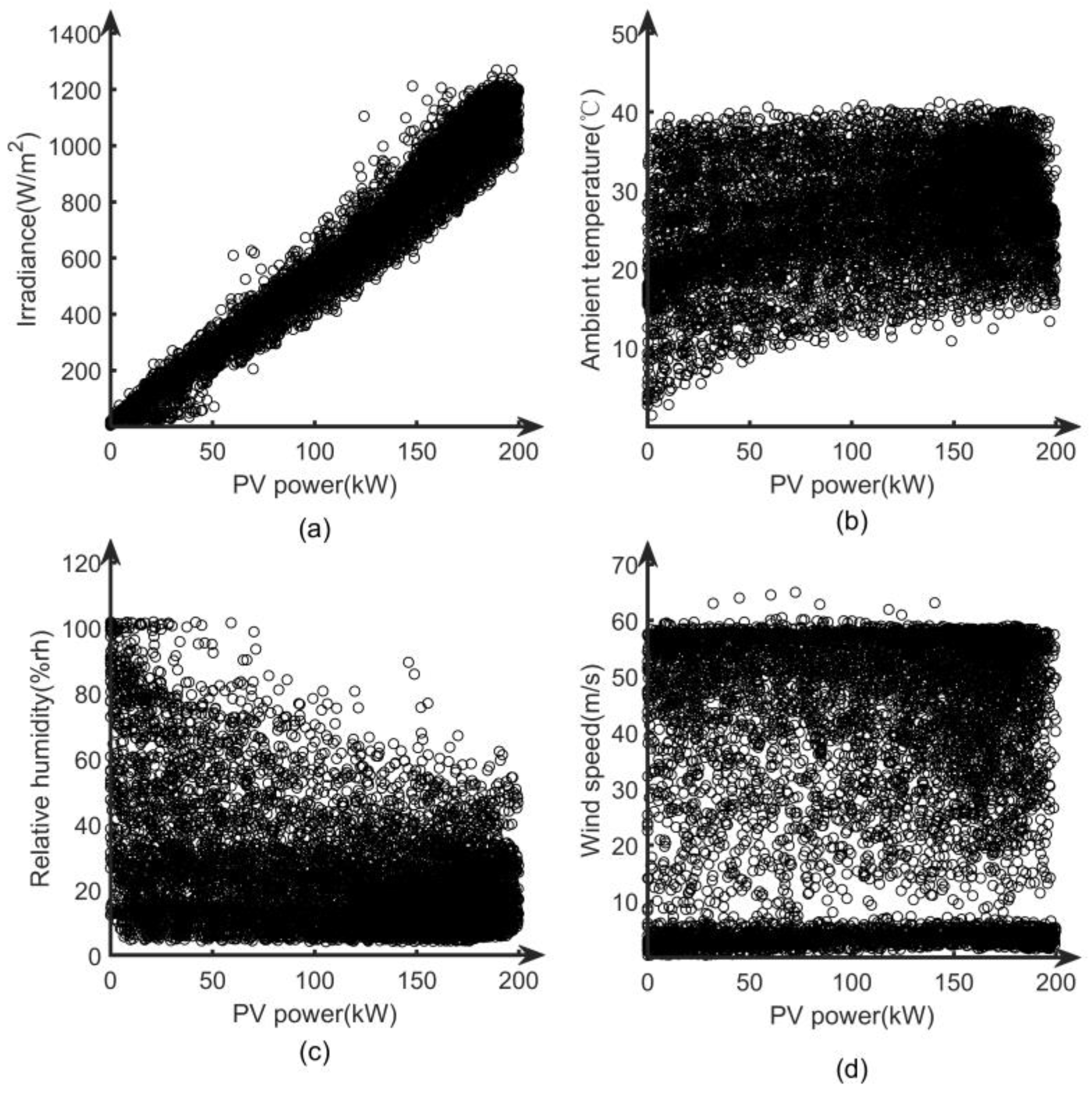
Five sets of characteristic variables from historical data, including PV power output, solar irradiance, ambient temperature, relative humidity, and wind speed are extracted. Through observation, it can be seen that these five sets of data are all continuous variables. Then, the scatter plot is used to sequentially determine whether the PV power output and the other four sets of variables meet linear correlation, as shown in Figure 2.

From Figure 2, it can be seen that the relationship between PV power and solar irradiance is linearly correlated, but not linearly correlated with ambient temperature, relative humidity, and wind speed. Therefore, the Spearman correlation coefficient method is selected to calculate the correlation [32]. The formula used is as follows：

ρ = \frac{\frac{1}{n} \sum_{i = 1}^{n} (R (x_{i}) - \bar{R (x)}) \cdot (R (y_{i}) - \bar{R (y)})}{\sqrt{(\frac{1}{n} \sum_{i = 1}^{n} {(R (x_{i}) - \bar{R (x)})}^{2}) \cdot (\frac{1}{n} \sum_{i = 1}^{n} {(R (y_{i}) - \bar{R (y)})}^{2})}}

(1)

where

ρ

is the Spearman correlation coefficient, n is the number of samples, x the value of a certain meteorological factor, and y is the PV power;

R (x_{i})

and

R (y_{i})

are the positional value of x and y, respectively;

\bar{R (x)}

and

\bar{R (y)}

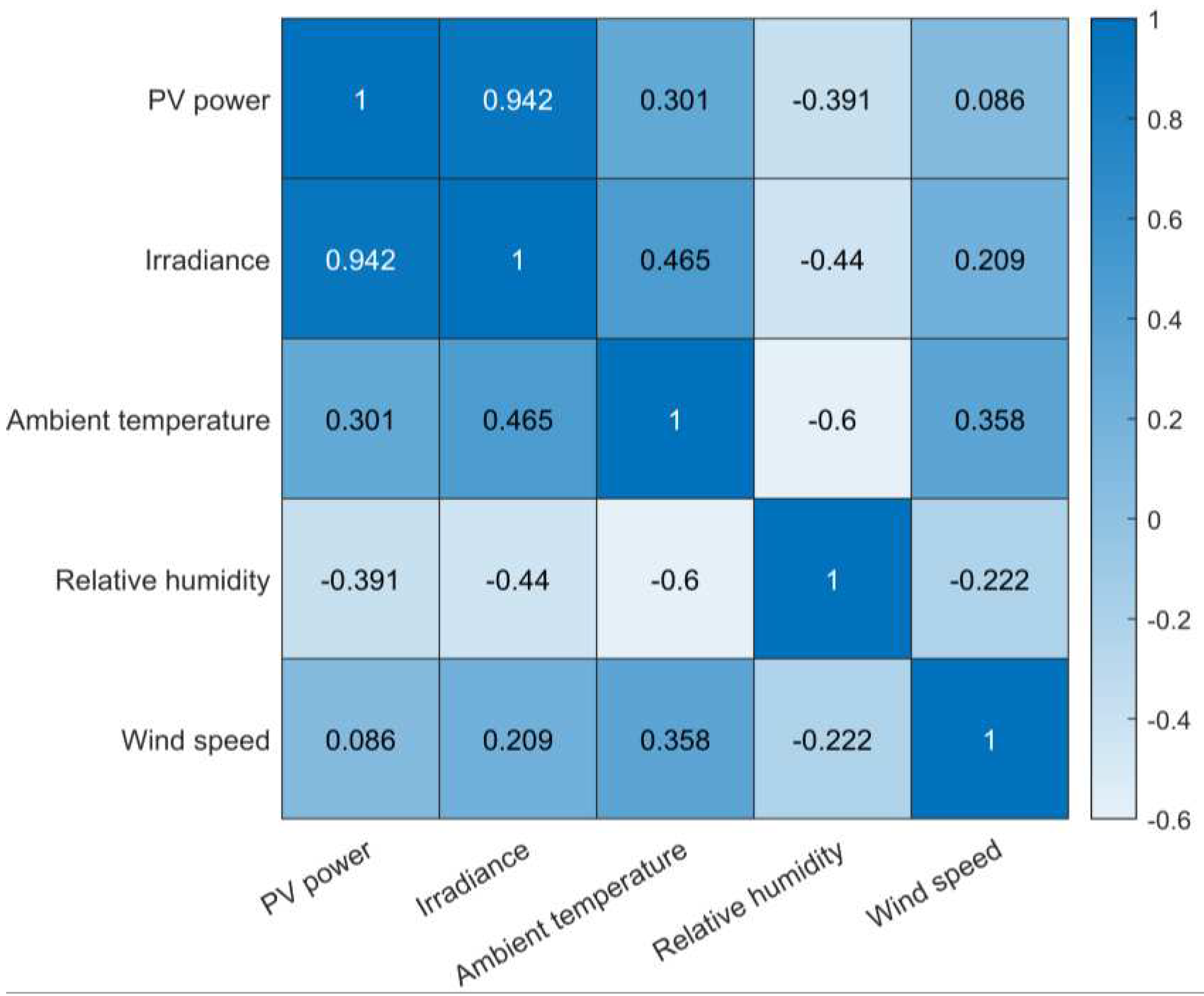
are the average positional value of x and y. The thermal diagram of the Spearman correlation coefficient between PV power and various meteorological features is shown in Figure 3.

As shown in Figure 3, the PV power is highly positively correlated with solar irradiance, positively correlated with environmental temperature, negatively correlated with relative humidity, and almost unrelated to wind speed. Therefore, solar irradiance, environmental temperature, and relative humidity are selected as the initial input features of the model in this paper.

2.4. Weather Category Construction

Due to the lack of direct indication of weather types in historical data, the K-means algorithm is used to classify weather types. The K-means algorithm is an iterative clustering analysis algorithm, whose main function is to automatically classify similar samples into corresponding categories. Compared with other classification algorithms, the K-means clustering algorithm is simpler and very effective. It can cluster sample data without prior knowledge of any sample conditions, and the reasonable determination of k values and initial cluster center points has a significant impact on the clustering effect [33,34].

Assuming that the given dataset X contains n objects, i.e.

X = \{X_{1}, X_{2}, X_{3}, \dots, X_{n}\}

, where each object has features of m dimensions. Firstly, initialize k cluster centers, and then calculate the Euclidean distance between each object and each cluster center. The calculation formula is as follows:

d i s (X_{i}, C_{j}) = \sqrt{\sum_{t = 1}^{m} {(X_{i t} - C_{j t})}^{2}}

(2)

where

X_{i}

represents the i-th object,

C_{j}

represents the j-th cluster center,

X_{i t}

represents the t-th feature of the i-th object, and

C_{j t}

represents the t-th feature of the j-th clustering center.

The distance from each object to each cluster center is compared in sequence, and the object to the nearest cluster center is assigned, then k clusters are obtained. The center of the cluster is the mean of all objects within the cluster in each feature, as shown in Eq.(3):

C_{l} = \frac{\sum_{X_{i} \in S_{l}} X_{i}}{|S_{l}|}

(3)

where

C_{l}

represents the l-th cluster center,

S_{l}

represents the l-th cluster,

|S_{l}|

represents the number of objects in the l-th cluster, and

X_{i}

represents the i-th object in the l-th cluster.

Based on the data of ambient temperature, relative humidity, and solar irradiance, the maximum, minimum, and average values of the above parameters on a single day are calculated as input parameters for K-means clustering. The initial value of k is set to 3. The clustering results of different seasons are obtained. The clustering centers in spring are shown in Table 1.

As shown in Table 1, for the clustering center of cluster 3, both the average ambient temperature and the average solar irradiance are the maximum, while the average relative humidity is the minimum; for the clustering center of cluster 2, both the average ambient temperature and solar irradiance are the minimum, while the average relative humidity is the maximum; and for the clustering center of cluster 1, the average values of each feature are in the middle. Therefore, cluster 1 belongs to the category of cloudy days, cluster 2 belongs to the category of rainy days, and cluster 3 belongs to the category of sunny days. Similarly, cluster the meteorological data for each season separately to obtain the number of different weather types for each season, as shown in Table 2.

As seen in Table 2, the number of rainy days is relatively small. To improve the accuracy of the model forecasting, the two weather types of cloudy and rainy days are merged as cloudy or rainy days.

2.5. Construction of the TLEL Model

2.5.1. Ensemble Learning

Ensemble learning is a method of constructing and combining multiple single learners to complete learning tasks. Firstly, multiple single weak learners are trained based on Boosting or Bagging learning methods, and then learning strategies such as averaging and voting are used to combine single weak learners to form a strong learner. The strong learners formed through ensemble learning have more significant generalization performance than single learners [17,35].

The single learner algorithms used in this paper include the XGBoost algorithm, RF algorithm, and CatBoost algorithm.

2.5.2. XGBoost Algorithm

XGBoost algorithm is an efficient gradient boosting decision tree（GBDT） algorithm, which is improved from the GBDT. As a forward addition model, it is one of the typical models of Boosting methods. This algorithm iteratively generates a new tree by fitting residuals, forming a classifier with higher accuracy and stronger generalization ability. The basic regression tree model used in the XGBoost model is represented as follows [36]:

\begin{matrix} {\hat{y}}_{i} = \sum_{t = 1}^{n} f_{t} (x_{i}), & f_{t} (x_{i}) \in R \end{matrix}

(4)

where n is the number of the trees,f_t is a function in the function space R,

{\hat{y}}_{i}

is the fore casting value of the regression tree, x_i is the i-th data input, and R is the set of all possible regression tree models.

A new function is added to the original model for each iteration. Every new function corresponds to a tree, and the newly generated tree fits the previous forecasting residual. The iterative process is as follows:

\{\begin{matrix} {\hat{y}}_{i}^{(0)} = 0 \\ {\hat{y}}_{i}^{(1)} = {\hat{y}}_{i}^{(0)} + f_{1} (x_{i}) \\ \cdot \cdot \cdot \\ {\hat{y}}_{i}^{(t)} = {\hat{y}}_{i}^{(t - 1)} + f_{t} (x_{i}) \end{matrix}

(5)

The objective function of the XGBoost model is shown in Eq. (6)：

X_{o b j} = \sum_{i = 1}^{n} l (y, \hat{y}) + \sum_{k = 1}^{n} Ω (f_{k})

(6)

where

\sum_{i = 1}^{n} l (y, \hat{y})

is the difference between the forecasting value of the model and the actual value, and

\sum_{k = 1}^{n} Ω (f_{k})

is the regular term of the scalar function.

The regularization penalty function is used to prevent overfitting of the model, as shown in Eq. (7):

Ω (f_{k}) = γ T + λ \frac{1}{2} \sum_{j = 1}^{T} ω_{j}^{2}

(7)

where T is the number of leaf nodes,

γ

is the penalty function coefficient,

ω

is the score of the leaf node, and

λ

is the regularization penalty coefficient.

The XGBoost model seeks to minimize the function objective through iteration. The formula for each iteration is as follows [37]:

τ^{(t)} = \sum_{j = 1}^{n} l (y_{i}, {\hat{y}}^{(t - 1)} + f_{t} (X_{i})) + Ω (f_{t})

(8)

To find one

f_{t}

that can minimize the objective function, the XGBoost model is expanded in the Taylor series at

f_{t} = 0

, and higher-order terms are ignored. The approximate expression of the objective function obtained is as follows:

τ^{(t)} \approx \sum_{j = 1}^{n} [l (y_{i}, {\hat{y}}^{(t - 1)} + f_{t} (X_{i})) + \frac{1}{2} h_{i} f_{t}^{2} (X_{i})] + Ω (f_{t})

(9)

2.5.3. RF Algorithm

The RF algorithm is an algorithm that integrates multiple trees through ensemble learning. Its basic unit is the decision tree, which is one of the typical models of Bagging methods. It can run effectively on large datasets and achieve good results for default value problems[37].

Assuming that the set S contains n different samples

\{x_{1}, x_{2}, \cdot \cdot \cdot, x_{n}\}

, and if one sample is extracted from the set S with replacement every time, a total of n times are extracted to form a new set

S^{*}

, the probability that the set

S^{*}

does not contain a certain sample

x_{i} (i = 1, 2, \cdot \cdot \cdot, n)

is presented as follows:

p = {(1 - \frac{1}{n})}^{n}

(10)

When

n \to \infty

，the value is as follows:

\lim_{n \to \infty} p = \lim_{n \to \infty} {(1 - \frac{1}{n})}^{n} = e^{- 1}

(11)

When constructing a decision tree, the RF algorithm uses the method of randomly selecting a split attribute set. Assuming the number of sample attributes is M, the specific process of the RF algorithm is as follows [38]:

Using the Bootstrap method to repeatedly sample and randomly generate T training sets $S_{1}, S_{2}, \cdot \cdot \cdot, S_{T}$ .
Using each training set $C_{1}, C_{2}, \cdot \cdot \cdot, C_{T}$ to generate a corresponding decision tree. Before selecting attributes on each non-leaf node, randomly select m attributes from the M attributes as the splitting attribute set for the current node, and split the node in the best splitting method among these m attributes.
Each tree grows well, so there is no need for pruning.
For the test set sample X, use each decision tree to test it and obtain the corresponding category $C_{1} (X), C_{2} (X), \cdot \cdot \cdot, C_{T} (X)$ .
Using the voting method, select the category with the highest output from T decision trees as the category to which sample X belongs.

2.5.4. CatBoost Algorithm

CatBoost algorithm is a gradient lifting algorithm based on decision tree improvement. Unlike traditional neural networks, it does not require a large number of samples as a training set and can perform high-accuracy forecasting based on small-scale samples. The CatBoost algorithm is one of the typical models of Boosting class methods. The CatBoost algorithm can solve the problem of overfitting in traditional GBDT algorithms. It reduces the impact of gradient estimation bias through unbiased gradient estimation, thereby improving the model's generalization ability [39].

In the traditional GBDT algorithm, the node splitting criterion is the label average value, while the CatBoost algorithm incorporates prior terms and weight coefficients to reduce the impact of noise and low-frequency category data on data distribution, as presented in Eq.(12):

{\hat{x}}_{k}^{i} = \frac{\sum_{j = 1}^{N} I_{\{x_{j}^{i} = x_{k}^{i}\}} y_{i} + a p}{\sum_{j = 1}^{N} I_{\{x_{j}^{i} = x_{k}^{i}\}} + a}

(12)

where

x_{k}^{i}

is the feature of the i-th category of the k-th training sample,

{\hat{x}}_{k}^{i}

is the average value of all

x_{k}^{i}

y_{i}

is the label of the j-th sample, I is the indicator function, p is the added prior term, and

a

is the weight coefficient.

A symmetric tree is used as a single learner. The same segmentation rule is applied at all layers in each iteration, while the left and right subtrees maintain symmetry balance. In a symmetric tree, the index of leaf nodes is encoded as a binary vector with a length equal to depth, and the corresponding binary features are stored in a continuous vector. The binary vector is represented as:

B_{x} = \sum_{m = 0}^{d - 1} 2^{m} B [x, f (t, m)]

(13)

where

B_{x}

is the binary vector established for sample x,

B [x, f (t, m)]

is the value of the binary eigenvalues of sample x read from vector B,

f (t, m)

is the number of binary features,

m

is the depth of the tree, and

t

is the number of trees.

2.5.5. LSTM Algorithm

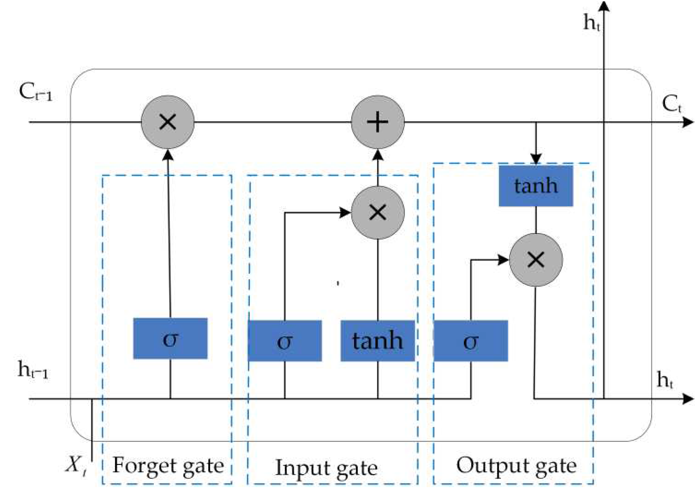
LSTM neural network is a temporal recurrent neural network that can solve the long-term dependency problem that exists in general recurrent neural networks. The LSTM neural network is composed of three parts: an input gate, an output gate, and a forget gate. The structural diagram is shown in Figure 4 [40,41].

The calculation formula for the information inside the LSTM cell is as follows [42]:

i_{t} = σ (W_{i} [x_{t}, h_{t - 1}] + b_{i})

(14)

{\tilde{c}}_{t} = \tanh (W_{c} [x_{t}, h_{t - 1}] + b_{c})

(15)

c_{t} = i_{i} \otimes {\tilde{c}}_{t} + f_{t} \otimes c_{t - 1}

(16)

f_{t} = σ (W_{f} [x_{t}, h_{t - 1}] + b_{f})

(17)

o_{t} = σ (W_{o} [x_{t}, h_{t - 1}] + b_{o})

(18)

h_{t} = o_{t} \tanh (c_{t})

(19)

where x_t is the input information at time t;

h_{t}

and

h_{t - 1}

are the output information at time t and t-1, respectively;

c_{t}

and

c_{t - 1}

represent the cell states at time t and t-1;

W

and

b

are the weight coefficients and deviations for each gate, respectively;

σ

and

\tanh

represent the activation function

s i g m o i d

and hyperbolic tangent activation function, respectively; f_t, i_t, and o_t are the state operation results of the forget gate, input gate, and output gate, respectively.

The input gate is used to control how much new information will be added to the cell state at each time t, that is, x_t and

h_{t - 1}

are processed by the

s i g m o i d

and

\tanh

functions respectively to jointly determine what information is stored in the memory cell state. The forget gate determines the proportion of cell state information that needs to be retained in the current cell state at time t-1. Moreover, the forget gate reads the information of h_t_-1 and x_t, if f_t was 0, all information of c_t_-1 will be discarded, and if f_t was 1, all information of c_t_-1 will be retained. The output gate determines the degree to which the c_t is saved to the cell output at time t.

2.5.6. TLEL Model

Considering the limitations of a single learner, this paper constructs the TLEL model based on ensemble learning using single learners' XGBoost, RF CatBoost, and LSTM models.

In the first layer of the TLEL model, the dataset that has been classified by weather categories and normalized is used as the input to perform hyperparameter optimization on the single learners' XGBoost, RF, and CatBoost models. Then the forecasting results of each model are combined as a subsequent forecasting dataset.

In the second layer of the TLEL model, the subsequent forecasting dataset obtained through the first layer is utilized as the input to perform hyperparameter optimization on the meta-learner LSTM model, and the forecasting results of the TLEL model are obtained. The forecasting result set is

f_{TLEL}

and the error data set is

e_{TLEL}

2.6. Construction of the Proposed FRD-TLEL Model

2.6.1. Feature Engineering

Feature Engineering is the process of transforming raw data into features that better express the essence of a problem, that is, discovering features that have a significant impact on the dependent variable to improve model performance[43,44]. The implementation methods include feature dimensionality reduction and the FRD methods.

In this paper, in addition to using the Spearman correlation coefficient to calculate correlation for feature dimensionality reduction, the use of the FRD method for machine learning is proposed, which trains the machine learning model by inputting a small number of influence features to obtain training results containing the model's features as new gain features for further training of the model. This method can not only preserve the value of the original features in the dataset but also achieve deep fusion between various models to improve model performance. This method can obtain data features through single-layer machine learning, with high efficiency in feature acquisition and full-carrying information.

2.6.2. FRD-TLEL Model

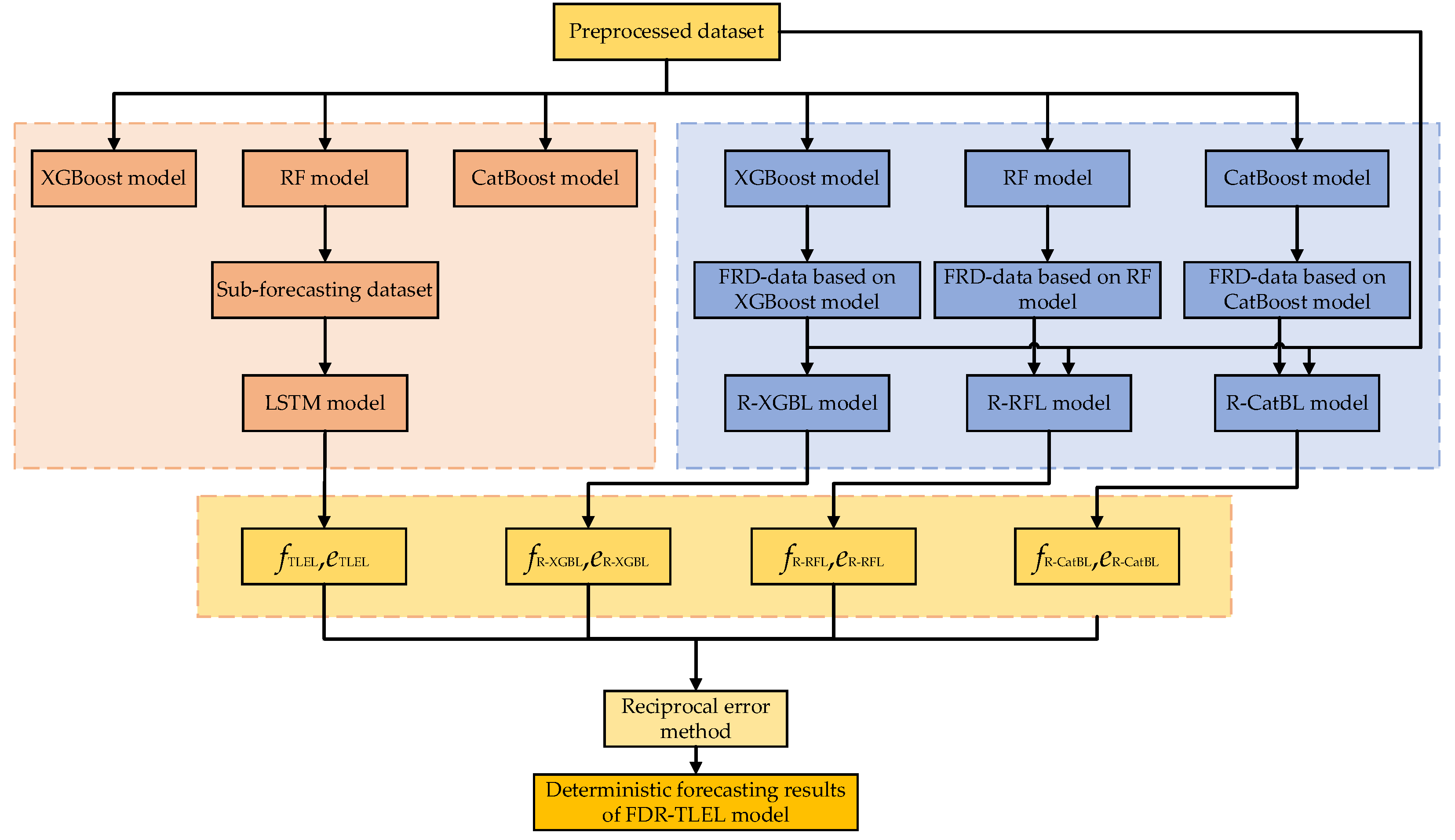
The FRD-TLEL model is proposed in this paper, whose framework is shown in Figure 5. Firstly, the XGBoost, RF, and CatBoost models are trained separately using the preprocessed dataset as input. Subsequently, the training results containing corresponding model features are obtained as new gain features, including the FRD data based on the XGBoost, RF, and CatBoost models, respectively. Secondly, hyperparameters are optimized for the corresponding LSTM model based on the new gain features and preprocessed dataset. Then the R-XGBL model, R-RFL model, and R-CatBL model are constructed. By constructing the R-XGBL model, the forecasting result set

f_{R - XGBL}

and error set

e_{R - XGBL}

are obtained. By constructing the R-RFL model, the forecasting result set

f_{R - RFL}

and error set

e_{R - RFL}

are obtained. By constructing the R-CatBL model, the forecasting result set

f_{R - CatBL}

and error set

e_{R - CatBL}

are obtained. Finally, the forecasting results of the TLEL, R-XGBL, R-RFL, and R-CatBL models are weighted and combined using the reciprocal error method to obtain the total forecasting results

f_{PV}

and errors

e_{PV}

f_{PV} = ω_{1} f_{1} + ω_{2} f_{2} + ω_{3} f_{3} + ω_{4} f_{4}

(20)

ω_{1} = \frac{e_{\max}}{e_{R - XGBL} + e_{R - CatBL} + e_{R - RFL} + e_{TLEL}}

(21)

ω_{2} = \frac{e_{\sec}}{e_{R - XGBL} + e_{R - CatBL} + e_{R - RFL} + e_{TLEL}}

(22)

ω_{3} = \frac{e_{thr}}{e_{R - XGBL} + e_{R - CatBL} + e_{R - RFL} + e_{TLEL}}

(23)

ω_{4} = \frac{e_{\min}}{e_{R - XGBL} + e_{R - CatBL} + e_{R - RFL} + e_{TLEL}}

(24)

e_{P V} = f_{A} - f_{P V}

(25)

where

ω_{i}

is the weight coefficient of the model;

e_{\min}

e_{\sec}

e_{thr}

and

e_{\max}

are the corresponding error values of

e_{TLEL}

e_{R - XGBL}

e_{R - RFL}

and

e_{R - CatBL}

sorted from small to large, respectively;

f_{1}

is the forecasting result set corresponding to

e_{\min}

f_{2}

is the forecasting result set corresponding to

e_{thr}

f_{3}

is the forecasting result set corresponding to

e_{\sec}

f_{4}

is the forecasting result set corresponding to

e_{\max}

, and

f_{A}

is the actual PV power. From Eq. (20) to (25), it can be seen that the reciprocal error method can amplify the advantages of small error models and reduce the disadvantages of large error models, thereby reducing the overall error of the combined model and achieving the goal of improving forecasting accuracy.

Figure 5. Framework of the FRD-TLEL model.

2.7. Probability Interval Forecasting Model Based on QR

The QR model can make up for the shortcomings of ordinary linear regression models. Compared with traditional least squares regression models, QR can better solve the problem of dispersed or asymmetric distribution of explanatory variables when the shape of the conditional distribution is unknown. It can meet the requirements of exploring the global distribution of response variables while studying the expected mean of response variables, and comprehensively describe the possible range of dependent variables.

The QR estimation is estimated using the weighted minimum absolute deviation sum method, which can ignore the influence of outliers. Its results are more stable, which can be used to describe the global features of response variables and thus mine richer information. The specific representation of QR model is as follows [45,46]:

\begin{matrix} Y = g_{τ} (β_{0, τ}^{T} X) + ε, & E [φ (ε)| X] = 0, & a . s . \end{matrix}

(26)

where X is a vector of p-dimensional covariates, Y is a real value response variable,

g_{τ} (·)

is an unknown univariate connection function,

φ (·)

is a known function, and

β_{0, τ}

is an index coefficient.

For the recognizability of the model, assume that

β_{0, τ}

satisfies

‖β_{0}‖ = 1

and the first component is positive. The expression for

β_{0, τ}

is as follows:

\begin{matrix} β_{0, τ} = \arg \min_{β} E [ρ_{τ} (Y - g (β_{0}^{T} X))], & ‖β‖ = 1, & β_{1} > 0 \end{matrix}

(27)

The loss function is shown in Eq.(28):

ρ_{τ} (u) = |u| + (2 τ - 1) u

(28)

Assuming

\{(X_{i}, Y_{i}), 1 \leq i \leq n\}

is an independent and identically distributed sample from (26), an estimate of

β_{0, τ}

can be obtained using the local linear method, represented as follows:

\hat{β} = \arg \min_{β} \min_{(a_{j}, b_{j})} \sum_{i = 1}^{n} \sum_{j = 1}^{n} ρ_{τ} (Y_{i} - a_{j} - b_{j} β^{T} X_{i j}) K (\frac{β^{T} X_{i j}}{h})

(29)

where

X_{i j} = X_{i} - X_{j}

，

K (·)

a kernel function, and h is bandwidth.

In this study, the steps for probability interval forecasting based on QR are as follows:

(1) Construction of interval forecasting models. Using the preprocessed dataset and the FRD-TLEL model-based short-term PV power deterministic forecasting error

e_{PV}

as inputs, a loss function

ρ_{τ} (u)

is set, and a QR interval forecasting model considering deterministic forecasting error is constructed.

(2) Forecasting of quantiles. In this step, we construct a quantile forecasting matrix, select quantiles, and perform quantile forecasting on PV power data based on the interval forecasting model established in step (1) to obtain forecasting results at different quantiles.

(3) The construction of forecasting intervals. The quantiles are selected to construct the upper and lower bounds of the PV power forecasting interval, thereby the forecasting intervals are generated at different confidence levels.

2.8. Performance Metrics

In this paper, for deterministic forecasting, two performance evaluation metrics, including mean absolute percentage error(MAPE) and the root mean square error (RMSE) [47,48], are employed to evaluate the forecasting results. MAPE is a measure of relative error that uses absolute values to avoid the cancellation of positive and negative errors. A smaller MAPE value indicates better model quality and more accurate forecasting. RMSE is the arithmetic square root of mean square error, reflecting the degree of deviation between the true value and the forecasting value. The smaller the RMSE value, the better the quality of the model and the more accurate the forecasting. These two performance metrics used for deterministic forecasting models can be expressed by Eqs. (30)-(31):

MAPE = \frac{100 %}{n} \sum_{i = 1}^{n} |\frac{{\hat{x}}_{i} - x_{i}}{x_{i}}|

(30)

RMSE = \sqrt{\frac{1}{n} \sum_{i = 1}^{n} {({\hat{x}}_{i} - x_{i})}^{2}}

(31)

where

{\hat{x}}_{i}

is the forecasting value of the model,

x_{i}

is the actual value of PV power , and

n

is the number of samples.

In this paper, for probabilistic interval forecasting, the performance metrics consist of prediction interval coverage percentage (PICP) and prediction interval normalized average width (PINAW) [49,50], which are indicated as follows:

PICP = \frac{1}{n} \sum_{i = 1}^{n} B^{(μ)}

(32)

PINAW = \frac{\sum_{i = 1}^{n} Δ P_{i}}{n}

(33)

where B is a Boolean quantity; if the actual power value is within the range, the value of B is 1, otherwise it is 0;

Δ P_{i}

is the bandwidth of the i-th interval.

PICP is used to evaluate the accuracy of the forecasting interval. The larger the PICP value, the higher the accuracy of the model's forecasting. PINAW is employed to evaluate the width of the interval. The smaller the PINAW value, the narrower the upper and lower boundary range of the model's forecasting.

3. Forecasting Results and Discussion

In this section, the preprocessed dataset that has undergone data cleaning, correlation analysis, weather category construction, normalization, and classification of training and test sets is input into the proposed FRD-TLEL model for deterministic forecasting. The forecasting results of the proposed model under different seasons and weather types are compared with those of other models. Then perform probability interval forecasting and compare the interval forecasting results under different confidence levels, seasons, and weather types. The detailed findings and discussions are provided below.

3.1. Analysis of Deterministic Forecasting Results

To verify the feasibility of the FRD-TLEL model proposed in this paper, the forecasting results of this model are compared with XGBoost, RF, CatBoost, LSTM, R-XGBL, R-RFL, R-CatBL, and TLEL models. A total of 31365 sets of data are selected as the training set from April 1, 2016, to May 1, 2018. In various clusters, data from a certain day in 2017 are randomly selected as the test set. Among them, November 18th is a sunny day in spring, and October 22nd is a cloudy or rainy day in spring; February 26th is a sunny day in summer, and December 21st is a cloudy or rainy day in summer; March 30th is a sunny day in autumn, and May 5th is a cloudy or rainy day in autumn; August 30th is a sunny day in winter, and July 25th is a cloudy or rainy day in winter. 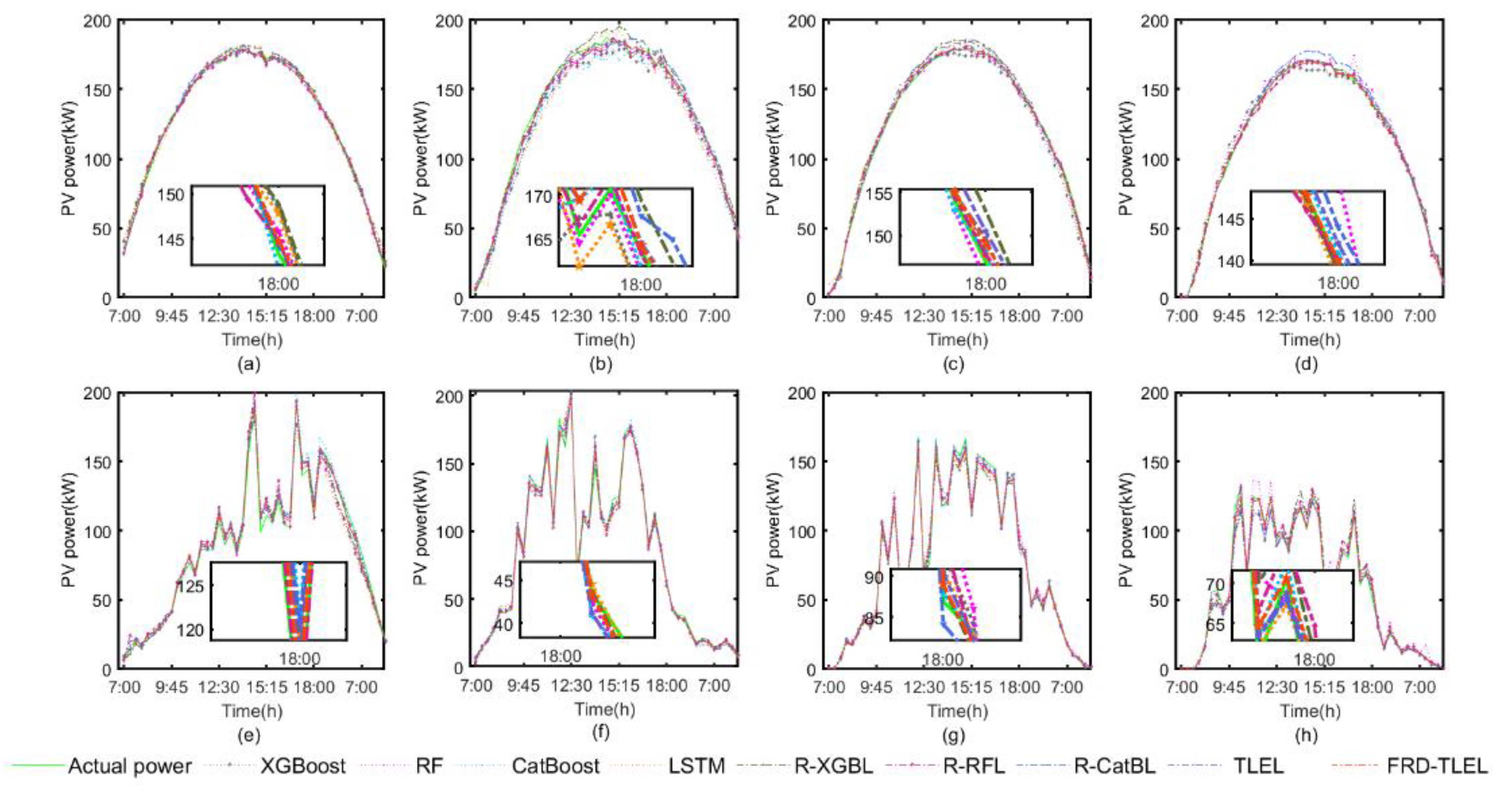Figure 6 shows the comparison between the deterministic forecasting results of the FRD-TLEL, XGBoost, RF, CatBoost, LSTM, R-XGBL, R-RFL, R-CatBL, and TLEL models, and the actual PV power under different weather types in each season.

From Figure 6, it can be seen that the shapes of the PV power curves on sunny days in each season all rise first and then fall, and the overall distribution is smooth, with occasional slight fluctuations. On cloudy or rainy days in each season, the PV power curves are distributed in a large fluctuation curve. The forecasting curves of different weather types in different seasons reflect that the deterministic forecasting results of the FRD-TLEL model are closer to the actual value than those of other models, and the forecasting accuracy of the TLEL model is better than that of every single model.

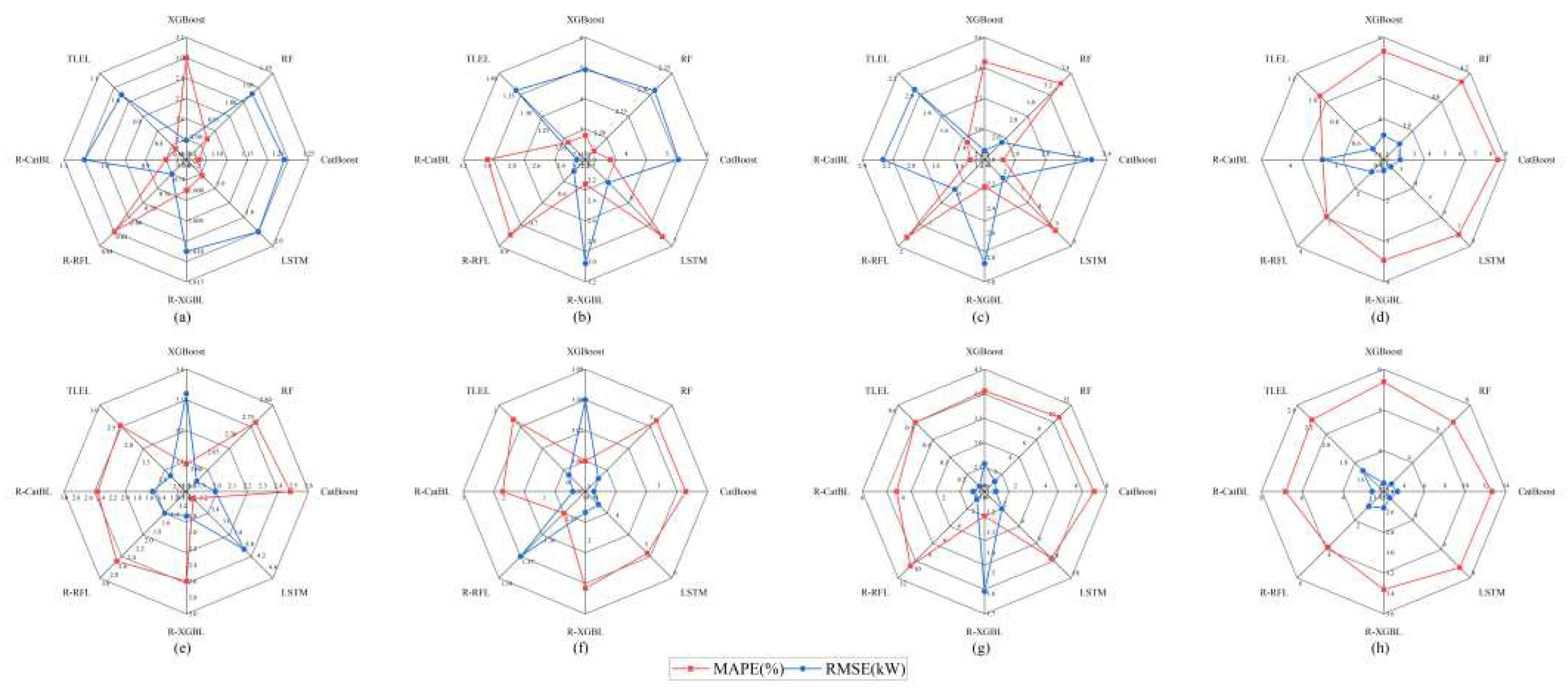
The error comparison of different forecasting methods on sunny days in different seasons is shown in Table 3, and the error comparison of different forecasting methods on cloudy or rainy days in different seasons is presented in Table 4. The decrease in performance metrics of the FRD-TLEL model compared to the other 8 models under different seasons and weather types is shown in Figure 7.

As shown in Table 3 and Table 4, and Figure 7, compared with XGBoost, RF, CatBoost, LSTM, R-XGBL, R-RFL, R-CatBL, and TLEL models, the FRD-TLEL model has the lowest MAPE and RMSE and has the best forecasting performance. It has a significant advantage in sunny weather; In cloudy or rainy weather, due to significant fluctuations of the meteorological factors, the stability of PV power is reduced, and its forecasting accuracy is slightly lower than that of sunny weather, but it is still within an acceptable range. Compared with each single model, the TLEL model has higher forecasting accuracy than the single models without the FRD method.

Taking the sunny day in spring as an example, in comparison with XGBoost, RF, CatBoost, LSTM, R-XGBL, R-RFL, R-CatBL, and TLEL models, the MAPE of the FRD-TLEL model decreased by 3%, 0.91%, 1.07%, 1.51%, 1.6%, 0.82%, 0.85%, and 0.75%, respectively, while the RMSE decreased by 2.19 kW, 1.04 kW, 1.21 kW, 1.9 kW, 1.61 kW, 0.74 kW, 1.05 kW and 1 kW, respectively. Compared with the single models XGBoost, RF, CatBoost, and LSTM, the MAPE of the TLEL model is reduced by 2.25%, 0.16%, 0.32% and 0.76%, and the RMSE is reduced by 1.19kW, 0.04kW, 0.21kW and 0.9kW, respectively.

On the rainy days in spring, in comparison with XGBoost, RF, CatBoost, LSTM, R-XGBL, R-RFL, R-CatBL, and TLEL models, the MAPE of the FRD-TLEL model decreased by 3.09%, 2.75%, 2.48%, 3.12%, 2.6%, 2.61%, 2.45% and 2.41%, respectively, while the RMSE decreased by 3.32kW, 2.58kW, 1.99kW, 4kW, 1.81kW, 1.5kW, 1.55kW and 0.96kW, respectively. Compared with XGBoost, RF, CatBoost, and LSTM, the MAPE of TLEL is reduced by 0.68%, 0.34% 0.07%, and 0.71%, respectively, and the RMSE is reduced by 2.36 kW, 1.62 kW, 1.03 kW, and 3.04 kW, respectively.

3.2. Analysis of Probability Interval Forecasting Results

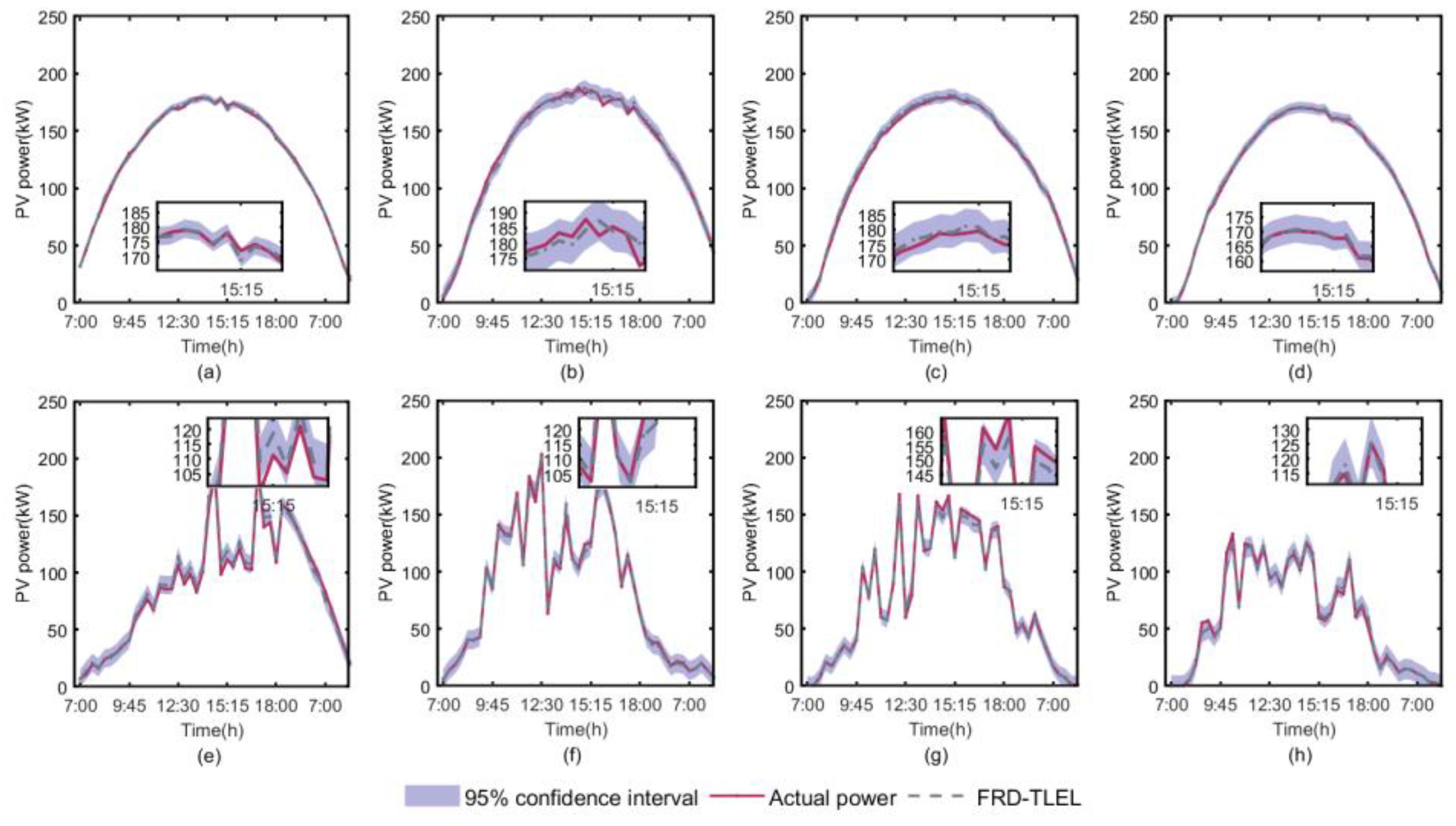
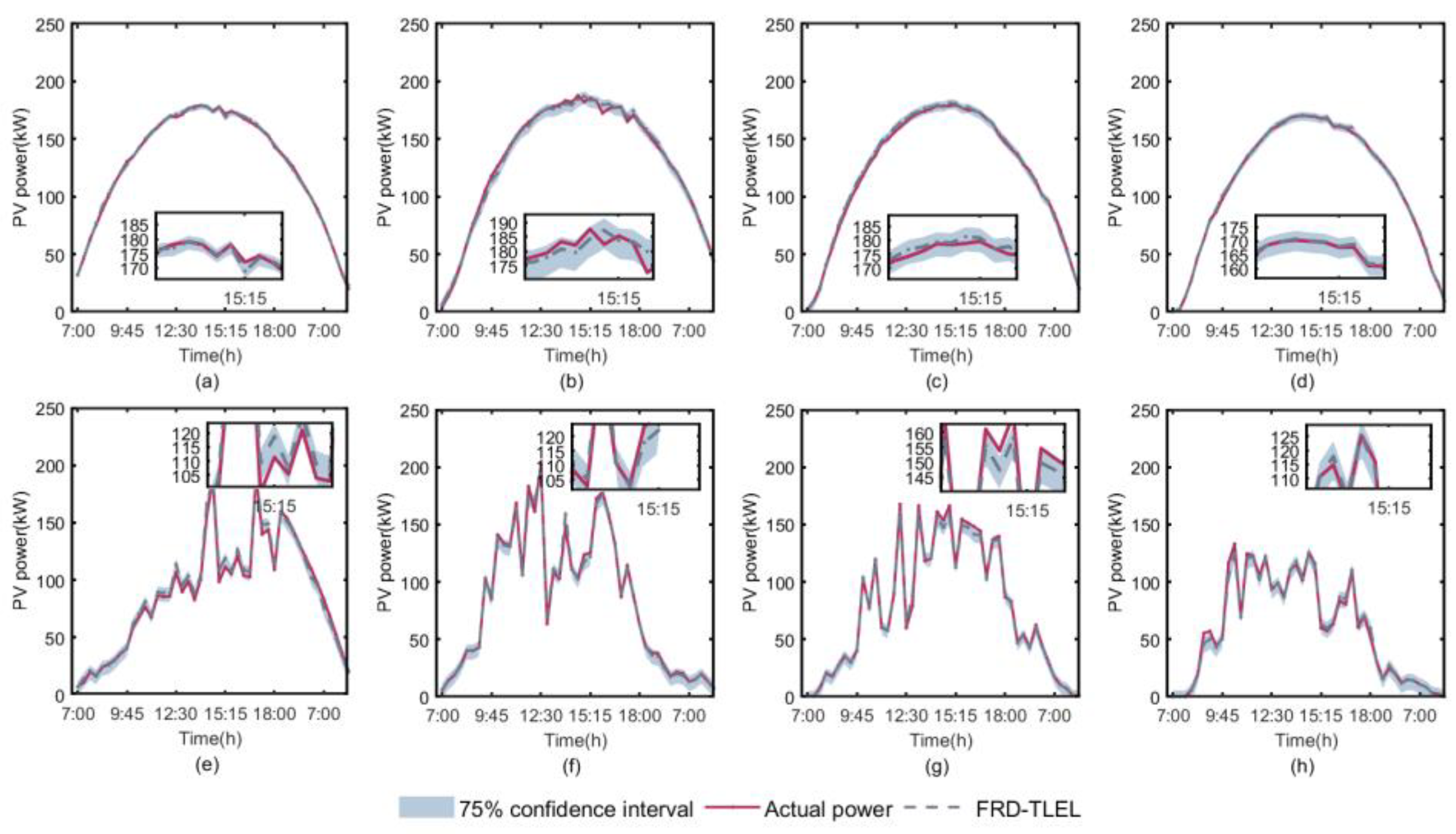
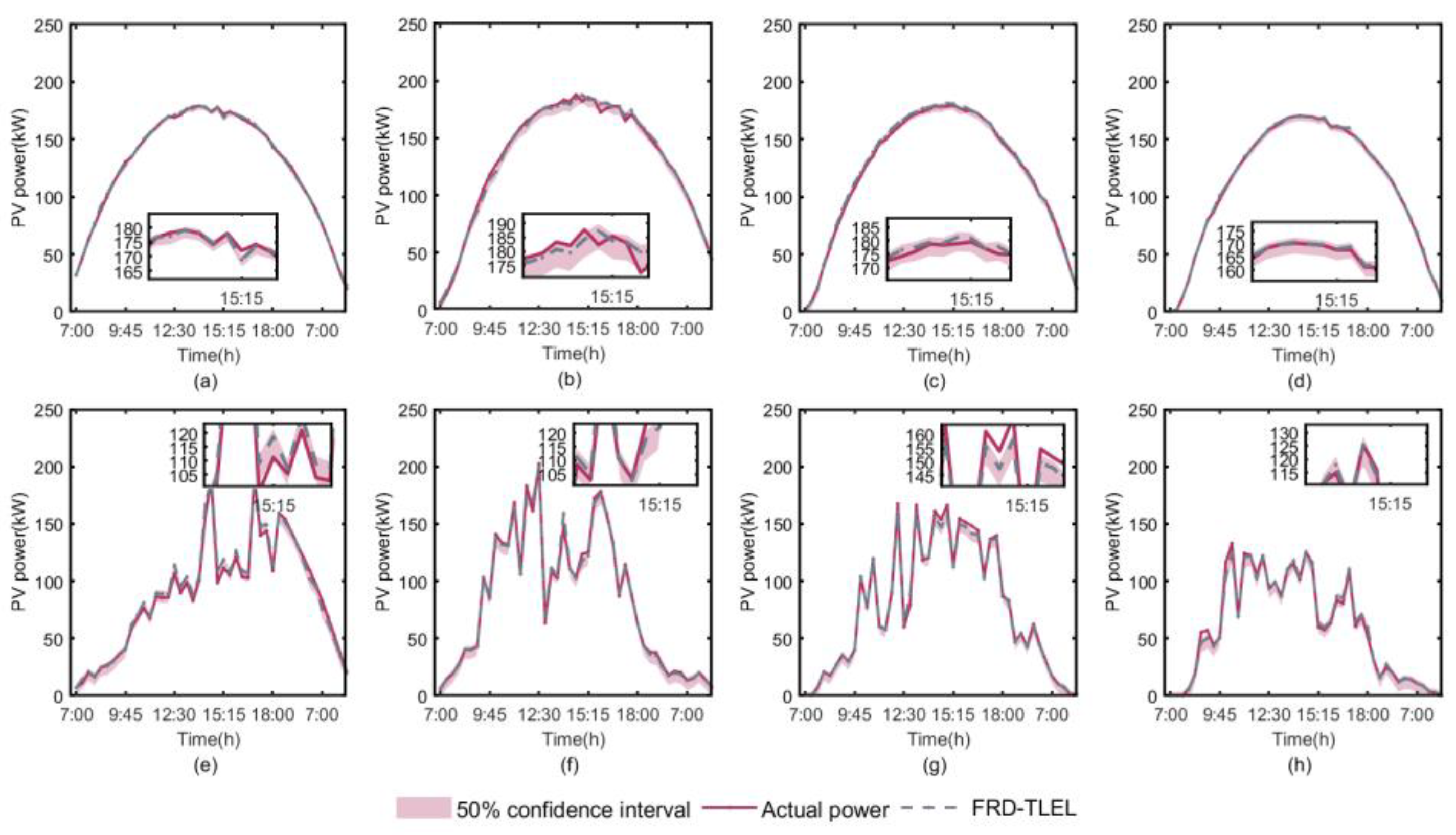
By combining the deterministic forecasting results of the FRD-TLEL model with QR estimation, interval forecasting of PV power is made for different seasons and weather types. The interval forecasting curves of PV power under 95%, 75%, and 50% confidence levels are obtained for sunny weather and cloudy or rainy weather in each season, as shown in Figure 8, Figure 9 and Figure 10.

According to Figure 8, Figure 9 and Figure 10 and Table 5, it is clear that the PICP levels for each season and weather type at 95%, 75%, and 50% confidence levels are higher than their basic confidence level, meeting the confidence conditions for interval forecasting. The PICP and PINAW of interval forecasting results for each season and weather type decrease with the decrease of confidence level. At a 95% confidence level, the interval PINAW is the largest and PICP is the highest, while at a 50% confidence level, the interval PINAW is the narrowest and PICP is the lowest.

4. Conclusions

In this paper, a novel FRD-TLEL model is proposed for short-term deterministic forecasting and probability interval forecasting of PV power. The main conclusions are summarized as follows:

By introducing the ensemble learning method into the proposed forecasting model, the limitations of a single forecasting model are changed and the forecasting accuracy is improved. Based on XGBoost, RF, CatBoost, and LSTM models, the TLEL model for short-term PV power deterministic forecasting is constructed by using the ensemble learning method. The forecasting results show that the TLEL model has lower MAPE and RMSE than a single model.
The introduction of the FRD method in the proposed forecasting model has improved the model's forecasting accuracy and efficiency. By inputting a small number of influential features to train each single model, the training results containing the model features are obtained, thus forming new gain features for further training of the models. This method can preserve the value of the original features in the dataset and achieve deep fusion between various models to improve model forecasting accuracy. In addition, in this method, data features can be obtained through a single machine learning model, with high feature acquisition efficiency and full carrying information.
The forecasting results verify that the proposed FRD-TLEL model is suitable for deterministic forecasting and probability interval forecasting of PV power in different seasons and weather types. In deterministic forecasting, compared with XGBoost, RF, CatBoost, LSTM, R-XGBL, R-RFL, R-CatBL, and TLEL models, the FRD-TLEL model has the minimum MAPE and RMSE in sunny weather and cloudy or rainy weather in spring, summer, autumn, and winter. Taking the sunny day in spring as an example, the MAPE of the proposed model decreased by the most to 3% compared to other models, and the RMSE decreased by the most to 2.19kW. This model has been applied to probability interval forecasting and shows good forecasting performance under different seasons and weather conditions at 95%, 75%, and 50% confidence levels.

In this study, during the data preprocessing phase, the data interpolation method is used to fill in the individual missing data. Although this method is simple and easy to understand, in rainy weather, due to changes in the meteorological environment, PV power and meteorological data may undergo significant changes in a short time period. At this time, the data interpolated using this method may have a marked deviation from the true value, which may have adverse effects on forecasting. How to process the data more finely is one of the feasible directions for our future research.

Author Contributions

Conceptualization, H.W. and J.W.; methodology, H.W. and S.Y.; software, H.W. and S.Y.; validation, S.Y. and D.J.; formal analysis, S.Y. and N.M.; investigation, J.F.; resources, S.W.; data curation, H.L.; writing—original draft preparation, H.W. and S.Y.; writing—review and editing, H.W. and J.W.; visualization, T.Z.; supervision, Y.X.; project administration, D.J.; funding acquisition, J.W. and H.W. All authors have read and agreed to the published version of the manuscript.

Funding

This research was supported by Liaoning Province Scientific Research Funding Program (LJKZ0681) and Science and the Technology Project in Electric Power Research Institute of State Grid Liaoning Electric Power Supply Co., Ltd. (2022YF-83).

Institutional Review Board Statement

Not applicable.

Data Availability Statement

Not applicable.

Acknowledgments

We thank the editors and reviewers for their helpful suggestions.

Conflicts of Interest

The authors declare no conflict of interest.

Nomenclature

PV	Photovoltaic
ARIMA	Autoregressive integral moving average algorithm
SVM	Support vector machine
RF	Random forest
DL	Deep learning algorithm
CNN	Convolutional neural network
Bi-LSTM	Bi-directional long short-term memory
RNN	Recurrent neural network
LSTM	Long-short-term memory
FRD-TLEL	Feature rise-dimensional two-layer ensemble learning
XGBoost	eXtreme Gradient Boosting algorithm
R-XGBL	FRD-XGBoost-LSTM
R-RFL	FRD-RF-LSTM
R-CatBL	FRD- CatBoost - LSTM
QR	Quantile regression
FCM	Fuzzy c-means clustering algorithm
WOA	White optimization algorithm
LSSVM	Least squares support vector machine model
ELM	Extreme learning machine
GRU	Gated recursive unit
KDE	Kernel density estimation
MAPE	Mean absolute percentage error
RMSE	Root mean square error
PICP	Prediction interval coverage percentage
PINAW	Prediction interval normalized average width

References

Abdellatif, A.; Mubarak, H.; Ahmad, S.; Ahmed, T.; Shafiullah, G.M.; Hammoudeh, A.; Abdellatef, H.; Rahman, M.M.; Gheni, H.M. Forecasting Photovoltaic Power Generation with a Stacking Ensemble Model. Sustainability 2022, 14, 11083. [Google Scholar] [CrossRef]
Zhou, W.; Jiang, H.; Chang, J. Forecasting Renewable Energy Generation Based on a Novel Dynamic Accumulation Grey Seasonal Model. Sustainability 2023, 15, 12188. [Google Scholar] [CrossRef]
Zhang, J.; Liu, Z.; Chen, T. Interval Prediction of Ultra-Short-Term Photovoltaic Power Based on a Hybrid Model. Electr. Power Syst. Res. 2023, 216, 109035. [Google Scholar] [CrossRef]
Das, U.K.; Tey, K.S.; Seyedmahmoudian, M.; Mekhilef, S.; Idris, M.Y.I.; Van Deventer, W.; Horan, B.; Stojcevski, A. Forecasting of Photovoltaic Power Generation and Model Optimization: A Review. Renew. Sustain. Energy Rev. 2018, 81, 912–928. [Google Scholar] [CrossRef]
Han, S.; Qiao, Y.; Yan, J.; Liu, Y.; Li, L.; Wang, Z. Mid-to-Long Term Wind and Photovoltaic Power Generation Prediction Based on Copula Function and Long Short Term Memory Network. Appl. Energy 2019, 239, 181–191. [Google Scholar] [CrossRef]
Tang, Y.; Yang, K.; Zhang, S.; Zhang, Z. Photovoltaic Power Forecasting: A Hybrid Deep Learning Model Incorporating Transfer Learning Strategy. Renew. Sustain. Energy Rev. 2022, 162, 112473. [Google Scholar] [CrossRef]
Niu, D.; Wang, K.; Sun, L.; Wu, J.; Xu, X. Short-Term Photovoltaic Power Generation Forecasting Based on Random Forest Feature Selection and CEEMD: A Case Study. Appl. Soft Comput. 2020, 93, 106389. [Google Scholar] [CrossRef]
Zhang, L.; He, Y.; Wu, H.; Yang, X.; Ding, M. Ultra-Short-Term Multi-Step Probability Interval Prediction of Photovoltaic Power: A Framework with Time-Series-Segment Feature Analysis. Sol. Energy 2023, 260, 71–82. [Google Scholar] [CrossRef]
Sobri, S.; Koohi-Kamali, S.; Rahim, N.A. Solar Photovoltaic Generation Forecasting Methods: A Review. Energy Convers. Manag. 2018, 156, 459–497. [Google Scholar] [CrossRef]
Mayer, M.J.; Gróf, G. Extensive Comparison of Physical Models for Photovoltaic Power Forecasting. Appl. Energy 2021, 283, 116239. [Google Scholar] [CrossRef]
Ahmed, R.; Sreeram, V.; Mishra, Y.; Arif, M.D. A Review and Evaluation of the State-of-the-Art in PV Solar Power Forecasting: Techniques and Optimization. Renew. Sustain. Energy Rev. 2020, 124, 109792. [Google Scholar] [CrossRef]
Antonanzas, J.; Osorio, N.; Escobar, R.; Urraca, R.; Martinez-de-Pison, F.J.; Antonanzas-Torres, F. Review of Photovoltaic Power Forecasting. Sol. Energy 2016, 136, 78–111. [Google Scholar] [CrossRef]
Wang, Z.; Wang, Y.; Cao, S.; Fan, S.; Zhang, Y.; Liu, Y. A Robust Spatial-Temporal Prediction Model for Photovoltaic Power Generation Based on Deep Learning. Comput. Electr. Eng. 2023, 110, 108784. [Google Scholar] [CrossRef]
Rafati, A.; Joorabian, M.; Mashhour, E.; Shaker, H.R. High Dimensional Very Short-Term Solar Power Forecasting Based on a Data-Driven Heuristic Method. Energy 2021, 219, 119647. [Google Scholar] [CrossRef]
Pan, M.; Li, C.; Gao, R.; Huang, Y.; You, H.; Gu, T.; Qin, F. Photovoltaic Power Forecasting Based on a Support Vector Machine with Improved Ant Colony Optimization. J. Clean. Prod. 2020, 277, 123948. [Google Scholar] [CrossRef]
Huang, X.; Li, Q.; Tai, Y.; Chen, Z.; Liu, J.; Shi, J.; Liu, W. Time Series Forecasting for Hourly Photovoltaic Power Using Conditional Generative Adversarial Network and Bi-LSTM. Energy 2022, 246, 123403. [Google Scholar] [CrossRef]
Banik, R.; Biswas, A. Improving Solar PV Prediction Performance with RF-CatBoost Ensemble: A Robust and Complementary Approach. Renew. Energy Focus 2023, 46, 207–221. [Google Scholar] [CrossRef]
Wang, F.; Xuan, Z.; Zhen, Z.; Li, K.; Wang, T.; Shi, M. A Day-Ahead PV Power Forecasting Method Based on LSTM-RNN Model and Time Correlation Modification under Partial Daily Pattern Prediction Framework. Energy Convers. Manag. 2020, 212, 112766. [Google Scholar] [CrossRef]
Guo, X.; Gao, Y.; Zheng, D.; Ning, Y.; Zhao, Q. Study on Short-Term Photovoltaic Power Prediction Model Based on the Stacking Ensemble Learning. Energy Rep. 2020, 6, 1424–1431. [Google Scholar] [CrossRef]
Wu, Y.-K.; Huang, C.-L.; Phan, Q.-T.; Li, Y.-Y. Completed Review of Various Solar Power Forecasting Techniques Considering Different Viewpoints. Energies 2022, 15, 3320. [Google Scholar] [CrossRef]
Li, P.; Zhou, K.; Lu, X.; Yang, S. A Hybrid Deep Learning Model for Short-Term PV Power Forecasting. Appl. Energy 2020, 259, 114216. [Google Scholar] [CrossRef]
Talaat, M.; Said, T.; Essa, M.A.; Hatata, A.Y. Integrated MFFNN-MVO Approach for PV Solar Power Forecasting Considering Thermal Effects and Environmental Conditions. Int. J. Electr. Power Energy Syst. 2022, 135, 107570. [Google Scholar] [CrossRef]
Liu, Y.; Liu, Y.; Cai, H.; Zhang, J. An Innovative Short-Term Multihorizon Photovoltaic Power Output Forecasting Method Based on Variational Mode Decomposition and a Capsule Convolutional Neural Network. Appl. Energy 2023, 343, 121139. [Google Scholar] [CrossRef]
Van Der Meer, D.W.; Widén, J.; Munkhammar, J. Review on Probabilistic Forecasting of Photovoltaic Power Production and Electricity Consumption. Renew. Sustain. Energy Rev. 2018, 81, 1484–1512. [Google Scholar] [CrossRef]
Liu, L.; Zhao, Y.; Chang, D.; Xie, J.; Ma, Z.; Sun, Q.; Yin, H.; Wennersten, R. Prediction of Short-Term PV Power Output and Uncertainty Analysis. Appl. Energy 2018, 228, 700–711. [Google Scholar] [CrossRef]
Li, K.; Wang, R.; Lei, H.; Zhang, T.; Liu, Y.; Zheng, X. Interval Prediction of Solar Power Using an Improved Bootstrap Method. Sol. Energy 2018, 159, 97–112. [Google Scholar] [CrossRef]
Mitrentsis, G.; Lens, H. An Interpretable Probabilistic Model for Short-Term Solar Power Forecasting Using Natural Gradient Boosting. Appl. Energy 2022, 309, 118473. [Google Scholar] [CrossRef]
Gu, B.; Shen, H.; Lei, X.; Hu, H.; Liu, X. Forecasting and Uncertainty Analysis of Day-Ahead Photovoltaic Power Using a Novel Forecasting Method. Appl. Energy 2021, 299, 117291. [Google Scholar] [CrossRef]
Long, H.; Zhang, C.; Geng, R.; Wu, Z.; Gu, W. A Combination Interval Prediction Model Based on Biased Convex Cost Function and Auto-Encoder in Solar Power Prediction. IEEE Trans. Sustain. Energy 2021, 12, 1561–1570. [Google Scholar] [CrossRef]
Pan, C.; Tan, J.; Feng, D. Prediction Intervals Estimation of Solar Generation Based on Gated Recurrent Unit and Kernel Density Estimation. Neurocomputing 2021, 453, 552–562. [Google Scholar] [CrossRef]
Available online: https://dkasolarcentre.com.au/.
Huang, C.; Yang, M. Memory Long and Short Term Time Series Network for Ultra-Short-Term Photovoltaic Power Forecasting. Energy 2023, 279, 127961. [Google Scholar] [CrossRef]
Liu, D.; Sun, K. Random Forest Solar Power Forecast Based on Classification Optimization. Energy 2019, 187, 115940. [Google Scholar] [CrossRef]
Zhen, Z.; Liu, J.; Zhang, Z.; Wang, F.; Chai, H.; Yu, Y.; Lu, X.; Wang, T.; Lin, Y. Deep Learning Based Surface Irradiance Mapping Model for Solar PV Power Forecasting Using Sky Image. IEEE Trans. Ind. Appl. 2020, 1–1. [Google Scholar] [CrossRef]
Khan, W.; Walker, S.; Zeiler, W. Improved Solar Photovoltaic Energy Generation Forecast Using Deep Learning-Based Ensemble Stacking Approach. Energy 2022, 240, 122812. [Google Scholar] [CrossRef]
Zhou, B.; Chen, X.; Li, G.; Gu, P.; Huang, J.; Yang, B. XGBoost–SFS and Double Nested Stacking Ensemble Model for Photovoltaic Power Forecasting under Variable Weather Conditions. Sustainability 2023, 15, 13146. [Google Scholar] [CrossRef]
Dai, Y.; Wang, Y.; Leng, M.; Yang, X.; Zhou, Q. LOWESS Smoothing and Random Forest Based GRU Model: A Short-Term Photovoltaic Power Generation Forecasting Method. Energy 2022, 256, 124661. [Google Scholar] [CrossRef]
Prasad, R.; Ali, M.; Kwan, P.; Khan, H. Designing a Multi-Stage Multivariate Empirical Mode Decomposition Coupled with Ant Colony Optimization and Random Forest Model to Forecast Monthly Solar Radiation. Appl. Energy 2019, 236, 778–792. [Google Scholar] [CrossRef]
Prokhorenkova, L.; Gusev, G.; Vorobev, A.; Dorogush, A.V.; Gulin, A. CatBoost: Unbiased Boosting with Categorical Features 2019.
Zhou, H.; Zhang, Y.; Yang, L.; Liu, Q.; Yan, K.; Du, Y. Short-Term Photovoltaic Power Forecasting Based on Long Short Term Memory Neural Network and Attention Mechanism. IEEE Access 2019, 7, 78063–78074. [Google Scholar] [CrossRef]
Gao, H.; Qiu, S.; Fang, J.; Ma, N.; Wang, J.; Cheng, K.; Wang, H.; Zhu, Y.; Hu, D.; Liu, H.; et al. Short-Term Prediction of PV Power Based on Combined Modal Decomposition and NARX-LSTM-LightGBM. Sustainability 2023, 15, 8266. [Google Scholar] [CrossRef]
Ospina, J.; Newaz, A.; Faruque, M.O. Forecasting of PV Plant Output Using Hybrid Wavelet-based LSTM-DNN Structure Model. IET Renew. Power Gener. 2019, 13, 1087–1095. [Google Scholar] [CrossRef]
Pirhooshyaran, M.; Scheinberg, K.; Snyder, L.V. Feature Engineering and Forecasting via Derivative-Free Optimization and Ensemble of Sequence-to-Sequence Networks with Applications in Renewable Energy. Energy 2020, 196, 117136. [Google Scholar] [CrossRef]
Salcedo-Sanz, S.; Cornejo-Bueno, L.; Prieto, L.; Paredes, D.; García-Herrera, R. Feature Selection in Machine Learning Prediction Systems for Renewable Energy Applications. Renew. Sustain. Energy Rev. 2018, 90, 728–741. [Google Scholar] [CrossRef]
Huang, Q.; Wei, S. Improved Quantile Convolutional Neural Network with Two-Stage Training for Daily-Ahead Probabilistic Forecasting of Photovoltaic Power. Energy Convers. Manag. 2020, 220, 113085. [Google Scholar] [CrossRef]
Hu, J.; Tang, J.; Lin, Y. A Novel Wind Power Probabilistic Forecasting Approach Based on Joint Quantile Regression and Multi-Objective Optimization. Renew. Energy 2020, 149, 141–164. [Google Scholar] [CrossRef]
Zhen, H.; Niu, D.; Wang, K.; Shi, Y.; Ji, Z.; Xu, X. Photovoltaic Power Forecasting Based on GA Improved Bi-LSTM in Microgrid without Meteorological Information. Energy 2021, 231, 120908. [Google Scholar] [CrossRef]
Ray, B.; Shah, R.; Islam, Md.R.; Islam, S. A New Data Driven Long-Term Solar Yield Analysis Model of Photovoltaic Power Plants. IEEE Access 2020, 8, 136223–136233. [Google Scholar] [CrossRef]
Yildiz, C.; Acikgoz, H.; Korkmaz, D.; Budak, U. An improved residual-based convolutional neural network for very short-term wind power forecasting. Energy Convers. Manag. 2021, 228, 113731. [Google Scholar] [CrossRef]
An, Y.; Dang, K.; Shi, X.; Jia, R.; Zhang, K.; Huang, Q. A Probabilistic Ensemble Prediction Method for PV Power in the Nonstationary Period. Energies 2021, 14, 859. [Google Scholar] [CrossRef]

Figure 1. The flowchart of the PV power forecasting.

Figure 2. Scatter plot of PV power with solar irradiance, ambient temperature, relative humidity, and wind speed. (a) Solar irradiance; (b) Ambient temperature; (c) Relative humidity; (d) Wind speed.

Figure 3. Thermal diagram of the Spearman correlation coefficient between PV power and var-ious meteorological factors.

Figure 4. The structure of the LSTM neural network.

Figure 6. Comparison of forecasting results of various models under different weather types in different seasons. (a) sunny day in spring; (b) sunny day in summer; (c) sunny day in autumn; (d) sunny day in winter; (e) cloudy or rainy day in spring; (f) cloudy or rainy day in summer; (g) cloudy or rainy day in autumn; (h) cloudy or rainy day in winter.

Figure 7. The decrease in performance metrics of the FRD-TLEL model compared to other models under different seasons and weather types. (a) sunny day in spring; (b) sunny day in summer; (c) sunny day in autumn; (d) sunny day in winter; (e) cloudy or rainy day in spring; (f) cloudy or rainy day in summer; (g) cloudy or rainy day in autumn; (h) cloudy or rainy day in winter.

Figure 8. Forecasting intervals for different seasons and weather types at a 95% confidence level. (a) sunny day in spring; (b) sunny day in summer; (c) sunny day in autumn; (d) sunny day in winter; (e) cloudy or rainy day in spring; (f) cloudy or rainy day in summer; (g) cloudy or rainy day in autumn; (h) cloudy or rainy day in winter.

Figure 9. Forecasting intervals for different seasons and weather types at a 75% confidence level. (a) sunny day in spring; (b) sunny day in summer; (c) sunny day in autumn; (d) sunny day in winter; (e) cloudy or rainy day in spring; (f) cloudy or rainy day in summer; (g) cloudy or rainy day in autumn; (h) cloudy or rainy day in winter.

Figure 10. Forecasting intervals for different seasons and weather types at 50% confidence level. (a) sunny day in spring; (b) sunny day in summer; (c) sunny day in autumn; (d) sunny day in winter; (e) cloudy or rainy day in spring; (f) cloudy or rainy day in summer; (g) cloudy or rainy day in autumn; (h) cloudy or rainy day in winter.

Table 1. Clustering centers in spring.

Feature	Cluster 1	Cluster 2	Cluster 3
Maximum ambient temperature（℃）	29.59	23.34	33.09
Minimum ambient temperature（℃）	14.72	16.01	18.54
Average ambient temperature（℃）	25.06	20.26	28.97
Maximum relative humidity（%rh）	57.32	67.30	40.23
Minimum relative humidity（%rh）	19.26	37.43	11.86
Average relative humidity（%rh）	29.92	50.70	18.32
Maximum solar irradiance（W/m²）	1054.96	551.19	1159.27
Minimum solar irradiance（W/m²）	26.01	18.61	84.03
Average solar irradiance（W/m²）	543.14	191.09	736.22

Table 2. Number of different weather types in each season.

Seasons	Sunny days	Cloudy days	Rainy days
Spring	88	71	20
Summer	127	33	20
Autumn	79	90	14
Winter	62	86	15

Table 3. The error comparison of different forecasting methods on sunny days in different seasons.

Seasons	Metrics	XGBoost	RF	CatBoost	LSTM	R-XGBL	R-RFL	R-CatBL	TLEL	FRD-TLEL
Spring	MAPE(%)	4.17	2.08	2.24	2.68	2.77	1.99	2.02	1.92	1.17
Spring	RMSE(kW)	3.56	2.41	2.58	3.27	2.98	2.11	2.42	2.37	1.37
Summer	MAPE(%)	5.34	4.72	6.16	9.33	4.79	3.31	5.55	3.75	2.55
Summer	RMSE(kW)	7.6	4.97	7.94	8.19	5.68	3.2	4.93	4.01	2.66
Autumn	MAPE(%)	5.86	5.7	4.14	7.51	4.64	4.12	3.94	3.82	2.42
Autumn	RMSE(kW)	4.91	4.65	4.35	4.11	4.9	2.08	4.28	4.06	2.05
Winter	MAPE(%)	6.69	5.17	9.49	8.23	4.5	4.01	4.33	2.02	1.03
Winter	RMSE(kW)	4.64	4.75	3.12	3.53	2.31	2.46	4.34	1.54	1.04

Table 4. The error comparison of different forecasting methods on cloudy or rainy days in different seasons.

Seasons	Metrics	XGBoost	RF	CatBoost	LSTM	R-XGBL	R-RFL	R-CatBL	TLEL	FRD-TLEL
Spring	MAPE(%)	7.63	7.29	7.02	7.66	7.14	7.15	6.99	6.95	4.54
Spring	RMSE(kW)	7.72	6.98	6.39	8.4	6.2	5.9	5.95	5.36	4.4
Summer	MAPE(%)	5.95	5.91	6.11	8.03	5.28	4.24	4.92	3.69	2.89
Summer	RMSE(kW)	6.3	5.57	5.69	6.67	4.99	4.59	3.53	3.25	3.22
Autumn	MAPE(%)	8.69	14.95	11.79	12.33	5.85	14.91	8.95	5.13	4.63
Autumn	RMSE(kW)	5.79	4.63	3.97	5.22	4.81	4.3	3.79	3.35	3.22
Winter	MAPE(%)	8.95	10.08	15.88	10.53	6.62	7.12	10.07	5.49	3.26
Winter	RMSE(kW)	6.59	5.92	6.73	5.81	5.94	4.41	5.95	5.02	3.38

Table 5. Interval forecasting performance metrics for different seasons and weather types at different confidence levels.

Confidence level	Weather type	Season	PICP	PINAW(%)
95%	Sunny day	Spring	1	0.15
		Summer	0.98	0.32
		Autumn	0.98	0.26
		Winter	0.98	0.23
	Cloudy or rainy day	Spring	0.93	0.37
		Summer	0.96	0.39
		Autumn	0.96	0.34
		Winter	0.96	0.41
75%	Sunny day	Spring	0.87	0.09
		Summer	0.91	0.19
		Autumn	0.89	0.15
		Winter	0.96	0.13
	Cloudy or rainy day	Spring	0.71	0.22
		Summer	0.89	0.23
		Autumn	0.82	0.2
		Winter	0.89	0.24
50%	Sunny day	Spring	0.56	0.05
		Summer	0.64	0.11
		Autumn	0.58	0.09
		Winter	0.93	0.08
	Cloudy or rainy day	Spring	0.52	0.13
		Summer	0.78	0.13
		Autumn	0.71	0.12
		Winter	0.8	0.14

Disclaimer/Publisher’s Note: The statements, opinions and data contained in all publications are solely those of the individual author(s) and contributor(s) and not of MDPI and/or the editor(s). MDPI and/or the editor(s) disclaim responsibility for any injury to people or property resulting from any ideas, methods, instructions or products referred to in the content.

© 2023 by the authors. Licensee MDPI, Basel, Switzerland. This article is an open access article distributed under the terms and conditions of the Creative Commons Attribution (CC BY) license (http://creativecommons.org/licenses/by/4.0/).

Copyright: This open access article is published under a Creative Commons CC BY 4.0 license, which permit the free download, distribution, and reuse, provided that the author and preprint are cited in any reuse.

MDPI Initiatives

Important Links

Choose an area of interest and we will send you notifications of new preprints at your preferred frequency.

Disclaimer

Short-Term Photovoltaic Power Forecasting Based on a Feature Rise-Dimensional Two-Layer Ensemble Learning Model

Abstract

1. Introduction

2. Methodology

2.1 Framework for Proposed Methods

2.2. Data Description

2.3. Correlation Analysis of Multiple Features

2.4. Weather Category Construction

2.5. Construction of the TLEL Model

2.5.1. Ensemble Learning

2.5.2. XGBoost Algorithm

2.5.3. RF Algorithm

2.5.4. CatBoost Algorithm

2.5.5. LSTM Algorithm

2.5.6. TLEL Model

2.6. Construction of the Proposed FRD-TLEL Model

2.6.1. Feature Engineering

2.6.2. FRD-TLEL Model

2.7. Probability Interval Forecasting Model Based on QR

2.8. Performance Metrics

3. Forecasting Results and Discussion

3.1. Analysis of Deterministic Forecasting Results

3.2. Analysis of Probability Interval Forecasting Results

4. Conclusions

Author Contributions

Funding

Institutional Review Board Statement

Data Availability Statement

Acknowledgments

Conflicts of Interest

Nomenclature

References

MDPI Initiatives

Important Links

Subscribe