1. Introduction
Floods triggered by extreme rainfall lead the rank of natural disasters in the Tropical Andes [
1,
2] causing huge damage to people’s lives and health, agricultural and systems production, economy, public and private infrastructure, etc. [
3,
4,
5]. Thus, flood modeling and forecasting are key to managing and preparing for extreme flood events, and also are valuable for timely flood warnings and emergency responses [
6,
7]. In that sense, the Andean population of Peru is highly prone and vulnerable to a large suite of extreme hydrometeorological events [
8,
9] such as higher rainfall rates in the eastern Andean/western Amazon transition [
10] and bigger water discharges from highlands to Andes foothills [
11]. For instance, extreme rainfalls and the subsequent floods that occurred in the austral summer of 2010 in Cusco (southern Peruvian Andes) caused US
$ 250 million in losses [
12] and evidence the crucial necessity for an accurate operational flood forecasting system [
13].
Hydrological forecasting aims to predict the system response from different input changes [
14] through processes of simplification that introduce uncertainties because of the limited system knowledge [
15,
16]. Forecasting uncertainties may evolve due to measurement errors [
17,
18], input errors [
19], structural errors [
20], parameter estimation errors [
21], and simulation errors [
22]. In that sense, Data Assimilation (DA) seeks the combinations of observation and model errors through the update of model states [
23].
To deal with that point, the following main steps are identified: a) design of the DA experiment scheme, b) quantification of model errors in the hydrological system, and c) application of the chosen DA algorithms into the Open Loop (OL) model. In the first case, data assimilation provides an effective way to integrate observation information. For example, real-time in situ measurements are increasingly being used to improve the estimations of forecast models via data assimilation techniques, and in many cases are readily available for operational systems [
24,
25,
26,
27,
28]. Hence, satellite remote sensing of soil moisture observations [
29] and snow cover data [
30] has been also integrated into assimilation frameworks in hydrological DA applications. Secondly, error quantification is a key process in DA applications. Modeling uncertainties in rainfall, states, and discharge may have a significant impact on results [
31,
32], even more than the selection of the DA algorithm [
33]. Finally, sequential assimilation of observation in the model with the Ensemble Kalman Filter (EnKF) and the Particle Filter (PF) is widely for probabilistic hydrologic predictions and skillful operational flood forecast systems [
34,
35,
36,
37].
Despite the advancements in streamflow DA worldwide in the last decade, the number of ensemble flood forecasting in South America is still emerging as highlighted by [
37,
38]. Most DA experiments have been applied in snow-dominated basins in the extratropical Andes using observed discharges [
38,
39] and remote sensing of snow cover [
40]; or incorporating satellite altimetry in the great Amazon basin [
41,
42,
43,
44].
In this context, flood forecasting in the Peruvian Tropical Andes is a challenging task due to a) the inaccessibility to remote areas with complex topography, b) the limited in-situ hydrometeorological network due to restricted funds, c) large amount of stations with short records (e.g. mostly of pluviometric automatic records begin on 2016) and huge number of missing values, and d) the raising uncertainties of model inputs related to the data-scarcity. Some studies in the Vilcanota River basin dealt with these issues by assessing near-real-time satellite precipitation products for rainfall-runoff modeling at sub-daily timesteps [
45], constraining structural errors in conceptual hydrological models [
45], and incorporating vegetation remote sensing into model calibration strategies [
46]. Hence, the improvement of accurate flood forecasts in a real-time hydrological system is still a pending task.
This paper aims the assess streamflow DA in a basin of the Tropical Andes of Peru using the EnKF and PF algorithms to assimilate real-time discharge observations into a sub-daily lumped flood forecasting system based on the GR4H model and driven by satellites-gauges merged rainfall estimations. We conduct the streamflow DA experiments in the Vilcanota River basin to compare streamflow forecast accuracy from 1 to 24 hours using the EnKF and PF.
2. Materials and Methods
2.1. Study Area
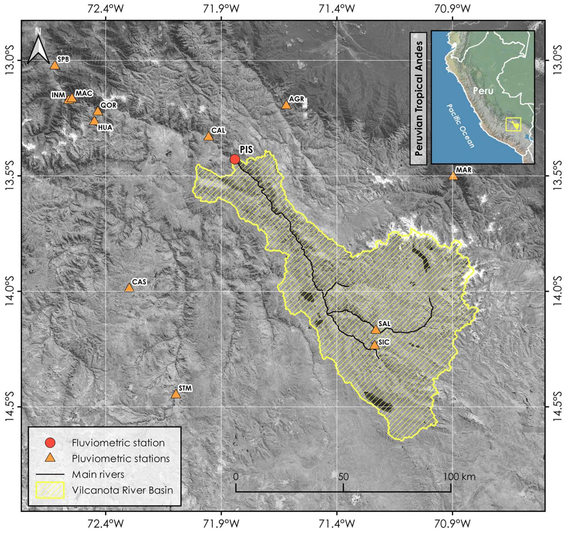
The study area comprises the Vilcanota River basin located in the southeastern Tropical Andes of Peru. This basin plays a key role in the economic-tourism activity of Cusco and was affected by extreme floods in 2010. For this work, we select a basin area delineated upstream of the Pisac fluviometric station (see
Figure 1). The drainage area of the basin is approximately 6900 km
2, spanning from 2959 m.a.s.l to 6268 m.a.s.l. Also, we defined a regular domain between latitudes 12.9 ºS — 14.8 ºS and longitudes 70.6 ºW — 72.7 ºW to download and merge satellite-based precipitation and pluviometric station observations in the study area.
The Vilcanota basin has a predominant pluvial regimen, with a smaller glacial/snow melting contribution to the total runoff volume.
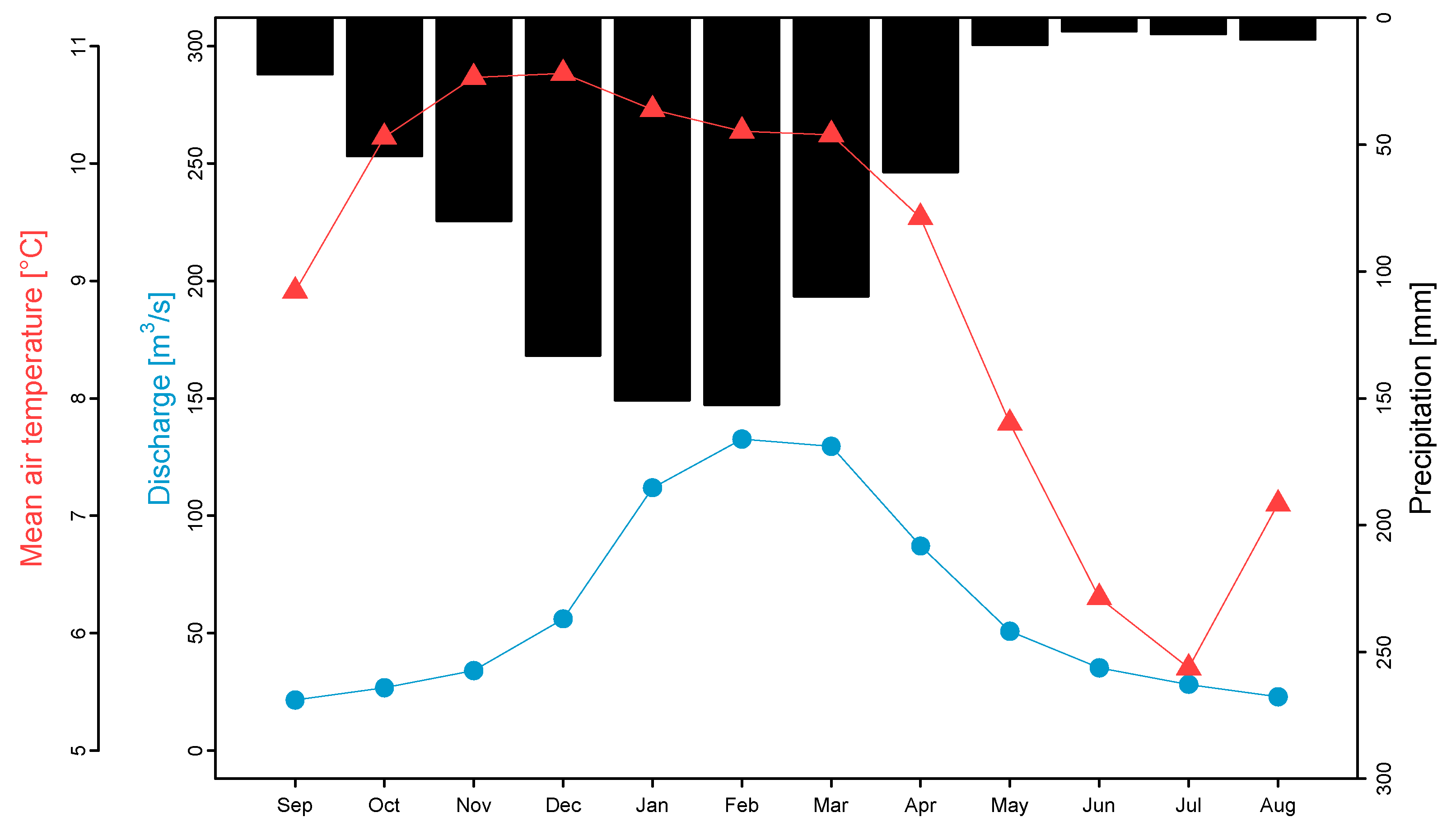
Figure 2 displays the seasonal behavior of the main hydroclimatic variables from September to August. Precipitation follows an unimodal distribution with rainfall rates ranging from 120 mm/month to 150 mm/month during the austral summer (December — March) and mean air temperature varies from 6 °C to 11 °C. Monthly discharges span from 20 m
3/s to 140 m
3/s, with peak flows often occurring in January and February.
Hourly discharge and rainfall records were collected from one fluviometric and 12 pluviometric gauge stations from 1
st January 2017 to 31
st July 2022. Stations owns to the National Service of Meteorology and Hydrology of Peru (SENAMHI). Gauge’s locations are displayed in
Figure 1 and summarized in
Table 1. Also, near-real-time Satellite Precipitation Products (SPPs) from the Integrated Multi-satellite Retrievals for GPM - Early Run (IMERG-E) and the Global Satellite Mapping of Precipitation (GSMaP-NRT) were chosen for this study. These SPPs have 5 hours of latency for UTC-5 with a spatial and temporal resolution of 0.1º (~10 km) and 0.5 hours, respectively. The process of merging SPPs and rain gauge information for the Vilcanota basin (IMERG-E’ and GSMaP-NRT’) is described in detail by [
45]. Additionally, hourly potential evapotranspiration was estimated based on the gridded evapotranspiration data set developed for Peru, called PISCOpe [
47].
2.2. Parsimonious Sub-daily Hydrological Modeling
The GR4H model [
48] is the hourly adaptation of the GR4J model [
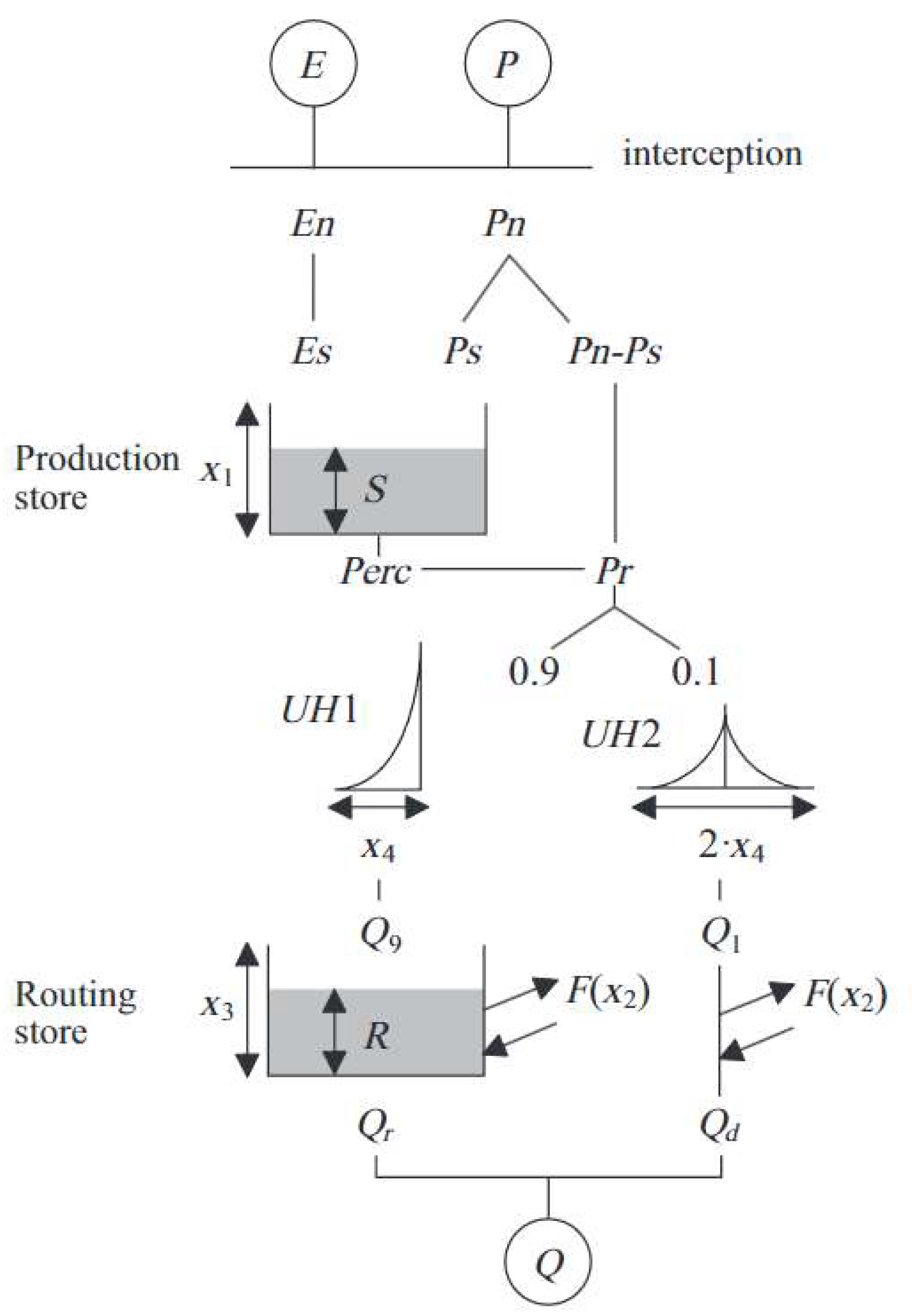
49] with four parameters (X1, X2, X3, and X4). The model structure is illustrated in
Figure 3. In this model, hourly precipitation and potential evapotranspiration are considered to determine the net precipitation (Pn) and evapotranspiration (En), respectively. Part of Pn is lost in the storage reservoir of the soil (Ps), while the remaining amount forms the effective precipitation (Pt = Pn - Ps). The soil moisture content (S), with a maximum value of X1, decreases due to percolation (Perc). Subsequently, Pt is routed at the basin outlet as follows: 10% is routed through a single unit hydrograph with a base time equal to X4, and the remaining 90% is routed through a unit hydrograph and a nonlinear reservoir (R) with a maximum capacity of X3. Additionally, a loss function (F), denoted by parameter X2, is applied to both flows to represent the subsurface exchange (loss or gain in the system).
The lumped GR4H models were forced using the merged IMERG-E’/GSMaP-NRT’ data and PISCOpe dataset at the basin scale. Models were calibrated and validated using observed hourly discharges at Pisac station. Calibration was conducted from the 00:00 hours of the 1st of January 2017 to the 23:00 hours of the 31st of August 2020. The first 1200 values were chosen for model warm-up. Model validation was from 00:00 hours on the 1st of September 2020 to 23:00 hours on the 31st of July 2022.
Model parameters were calibrated with the Shuffled Complex Evolutionary (SCE-UA) algorithm [
50] using the objective function (Fobj) proposed by [
28] and shown in equation 1.
Fobj is the arithmetic average of the logarithmic Nash Sutcliffe Efficiency (logNSE), the Box-Cox transformed Nash Sutcliffe Efficiency (BoxNSE), the Kling-Gupta Efficiency (KGE), and the BIAS. Details of the selected statistical metrics and their equations are summarized in
Table 2.
2.3. Design of Streamflow Data Assimilation Experiments
The sequential assimilation technique is well known for operational flood forecasting systems and is structured by adding normally distributed perturbations to the forcing vector [
51].
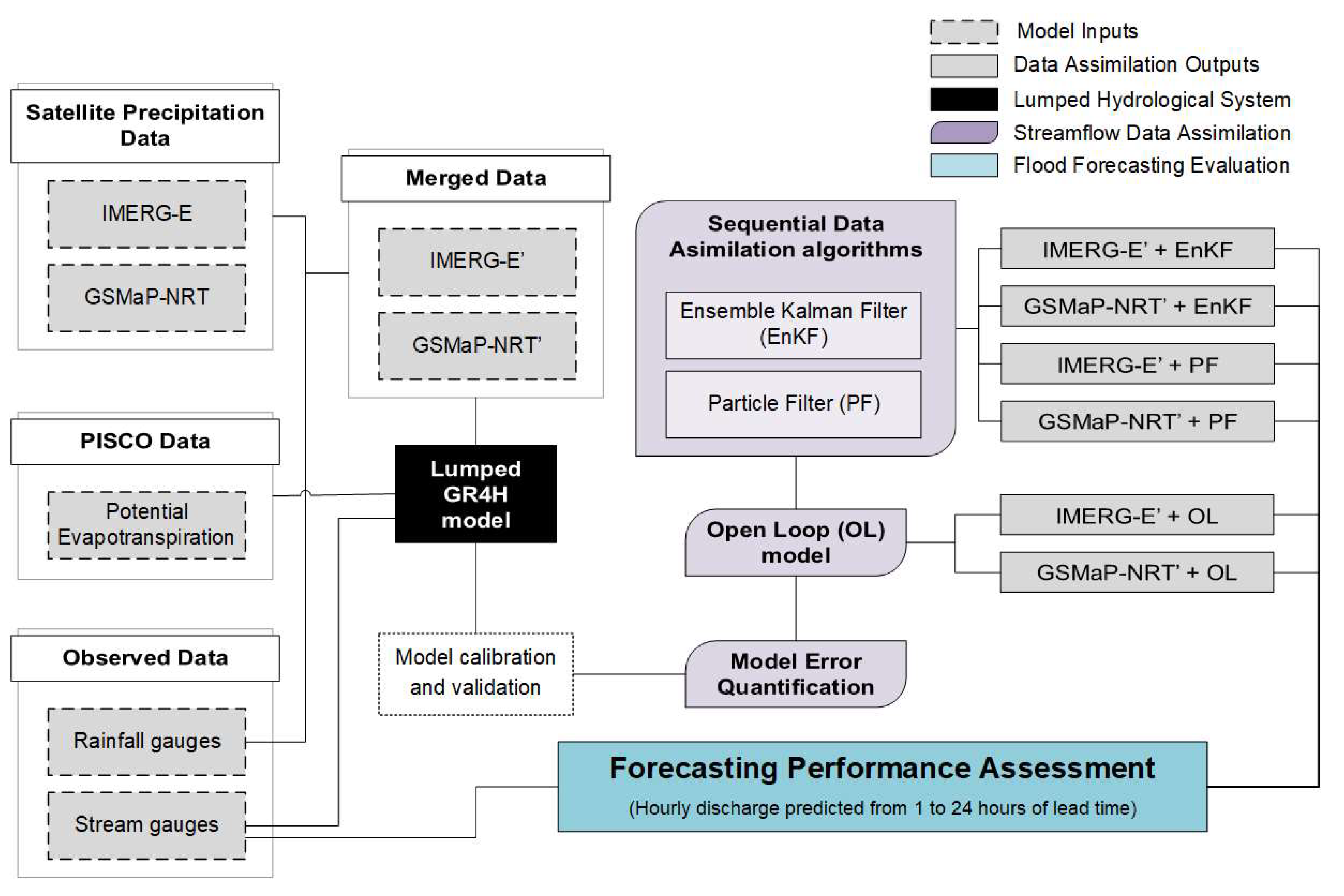
Figure 4 illustrates the general framework for streamflow DA in the Vilcanota River basin that starts with the quantification of model errors, runs the Open Loop model, and finishes with the application of DA algorithms.
To design stream DA experiments in this study, two Open Loop (OL) models were run forward using 100 ensemble members of precipitations and potential evapotranspiration data. Both OL schemes have the same potential evapotranspiration series from the PISCOpe dataset but differ in precipitation inputs. Thus, OL models are called IMERG-E’+OL and GSMaP-NRT’+OL, depending on the precipitation source used.
Also, we conducted four sequential DA experiments using the Ensemble Kalman Filter (EnKF) and the Particle Filter (PF) algorithms. The main difference between both algorithms is how they recursively generate an approximation to the probability distributions of the prognostic variables. EnKF assumes a Gaussian prior distribution for Kalman Gain and analysis states [
31]. Hence, PF updates importance weights according to the likelihood value of particles and observations, removing samples with negligible weights and replicating samples with large weights to avoid filter degeneracy [
35].
Same as OL experiments, we denominated experiments based on the precipitation source and algorithm chosen, so the IMERG-E’+EnKF and IMERG-E’+PF setups were run using IMERG-E’ inputs, while GSMaP-NRT’+EnKF and GSMaP-NRT’+PF used the GSMaP-NRT’ data.
These DA experiments were applied using an hourly adaptation of the R source code from the airGRdatassim package [
52].
2.4. Quantification of Model Errors
An ensemble of model realizations was generated to reflect the uncertainty in the catchment model. Rainfall (P) and evapotranspiration (E) inputs and basin soil moisture (S) were perturbed to generate an ensemble of model states and discharge predictions (Q). Also, the observed discharge was perturbed to represent the observation error. Similar to [
31], parameters and structural errors were assumed to be accumulated in soil moisture.
Ensemble meteorological inputs were generated by perturbing rainfall and evapotranspiration with multiplicative stochastic noise φ
p applied at each hourly time step, according to the methodology proposed by [
35] and presented in equations 2 and 3. Also, like [
52], random perturbations are provided by a first-order autoregressive model to guarantee temporal correlation of the time-variant forcings. The fractional error parameter was set to 0.65 and temporal decorrelations lengths were defined as 5 hours for rainfall and 3 hours for potential evapotranspiration based on an autocorrelation analysis.
where u
p is a uniform random number, such that φ
p is a realization from a uniform distribution ranging from 1-ε
p to 1+ε
p.
Basin soil moisture state (S) can be perturbed through normally distributed null-mean noise at each assimilation time step after the analysis procedure following the approach of [
53]. This perturbation was truncated by the upper (X1) and lower (zero) bounds of soil moisture.
According to [
35], errors in discharges are mainly from measurement of water level and uncertainties in rating curves. Here we use a normal distribution with a zero-valued mean and a variance (σ
obs2) for describing the measurement noise and parameterizing it as a function of the discharge observation (Q
obs) and presented in equation 4.
Following the approach proposed by [
32,
35,
39], the error parameter ε
obs was set to 0.1, the quantile 10 (Q
10) was used as the minimum threshold to prevent underestimated error variances in the case of low discharges, and the variance was evaluated proportionally to Q
102 for values below Q
10.
2.5. Evaluation of Model Forecast
We assess forecast performance during February and March 2022 for lead times from 1 to 24 hours. For this procedure, the updated (a posteriori) states of the GR4H model (S, R, HU1, and HU2) were taken as the baseline for flow forecasting from 1 to 24 hours. Here we use Nash-Sutcliffe Efficiency (NSE) and Bias (BIAS) to evaluate the mean ensemble forecast, the Mean of Ensemble Root Mean Squared Error (MRMSE), and the Continuous Ranked Probability Skill Score (CRPSS) to examine the ensemble spread. Details of statistical metrics and their equations are summarized in
Table 3.
3. Results
3.1. Model Calibration and Validation
Model parameters were calibrated for both precipitation sources (IMERG-E’ and GSMaP-NR’). Overall, the conceptual soil moisture (S) has a maximum capacity (x1) of 972 mm and the conceptual slow routing storage (R) has a reference capacity (x3) of 136 mm. The calibration process gives good results in terms of mass balance (BIAS), variance (KGE), and flow representation (logNSE, BoxNSE). The summary of statistical metrics selected for calibration, validation, and total period performance evaluation is shown in
Table 4.
Figure 5 displays the comparison between observed and simulated hourly discharges at the Pisac gauge station (basin outlet).
Figure 5a-b shows flow series (2017 – 2022) during the calibration and validation periods. Two different mean-areal precipitation inputs over the Vilcanota basin are shown in gray bars above their respective hydrographs. Observed discharge is present as blue lines and simulated discharges are plotted in green (IMERG-E') and magenta (GSMaP-NRT') lines. The dashed red box corresponds to the rainiest months in 2022 (February and March) selected for the streamflow DA assessment.
During the calibration and validation steps in
Figure 5a-b, the parsimonious GR4H model represents the high variability of discharges at hourly time step. Hence, peak flows are often underestimated during the wet period which increases positive BIAS. In terms of statistical metrics (
Table 4), simulations perform slightly better (logNSE, BoxNSE, and KGE higher than 0.85) when GR4H model is forced with IMERG-E' than GSMaP-NRT', even during model validation.
Overall,
Figure 5c-d shows scatter plots between observed and simulated values for February and March 2022. Simple Linear Regression model (SLR) for IMERG-E’ (green) and GSMaP-RT’ (magenta) simulations and Pearson Correlation are presented in the figures. Results here evidence that good calibration and validation skills do not always guarantee a good representation of discharges in short periods such as February and March 2022. The lower SRL’s slope values and Pearson correlation coefficients (R<0.50) indicate the subestimation and high dispersion of observed discharges, respectively; and are drastically noted for the GSMaP-NRT’ driven model.
3.2. Estimation of Model Uncertainties in Streamflow Data Assimilation
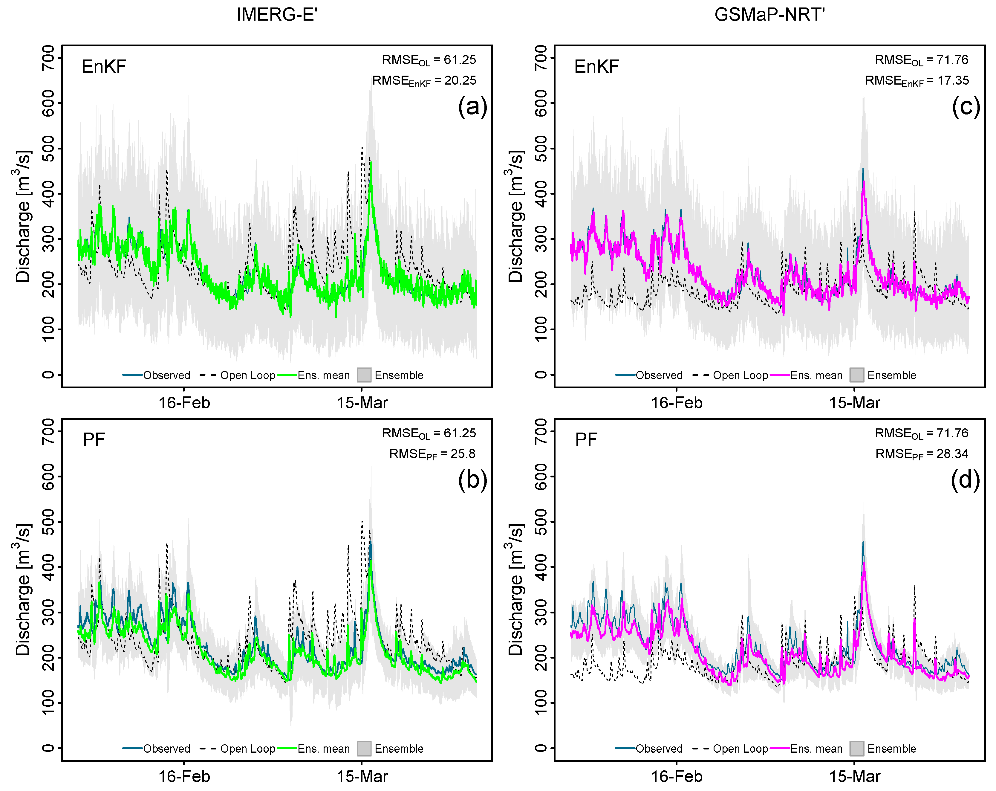
Figure 6 shows simulation results for the streamflow DA experiments, where blue lines correspond to hourly discharge observations, black lines represent OL model runs, green (magenta) lines display ensemble means streamflow simulations for IMERG-E’ (GSMaO-NRT’), and the ensemble spreads are shown as gray bounds.
The Root Mean Squared Error (RMSE) values in
Figure 6 quantify errors between simulated and observed discharges. In terms of RMSE, lower values indicate that IMERG-E’+OL (61.25 m
3/s) simulations perform better than GSMaP-NRT’+OL (71.76 m
3/s). However, after the application of DA algorithms (EnKF or PF), GSMaP-NRT’ driven experiments performed better than IMERG-E’ ones. Thus, the reduction of RMSE values is preliminary evidence of the benefits of streamflow DA to decrease model uncertainties in the Vilcanota basin. Concerning the algorithms used, the EnKF has a better performance than PF. For instance, the GSMaP-NRT'+EnKF scheme has the lowest RMSE value (17.35 m
3/s). Hence, for an ensemble size of 100 members, the ensemble spreads in PF experiments are thinner than EnKF.
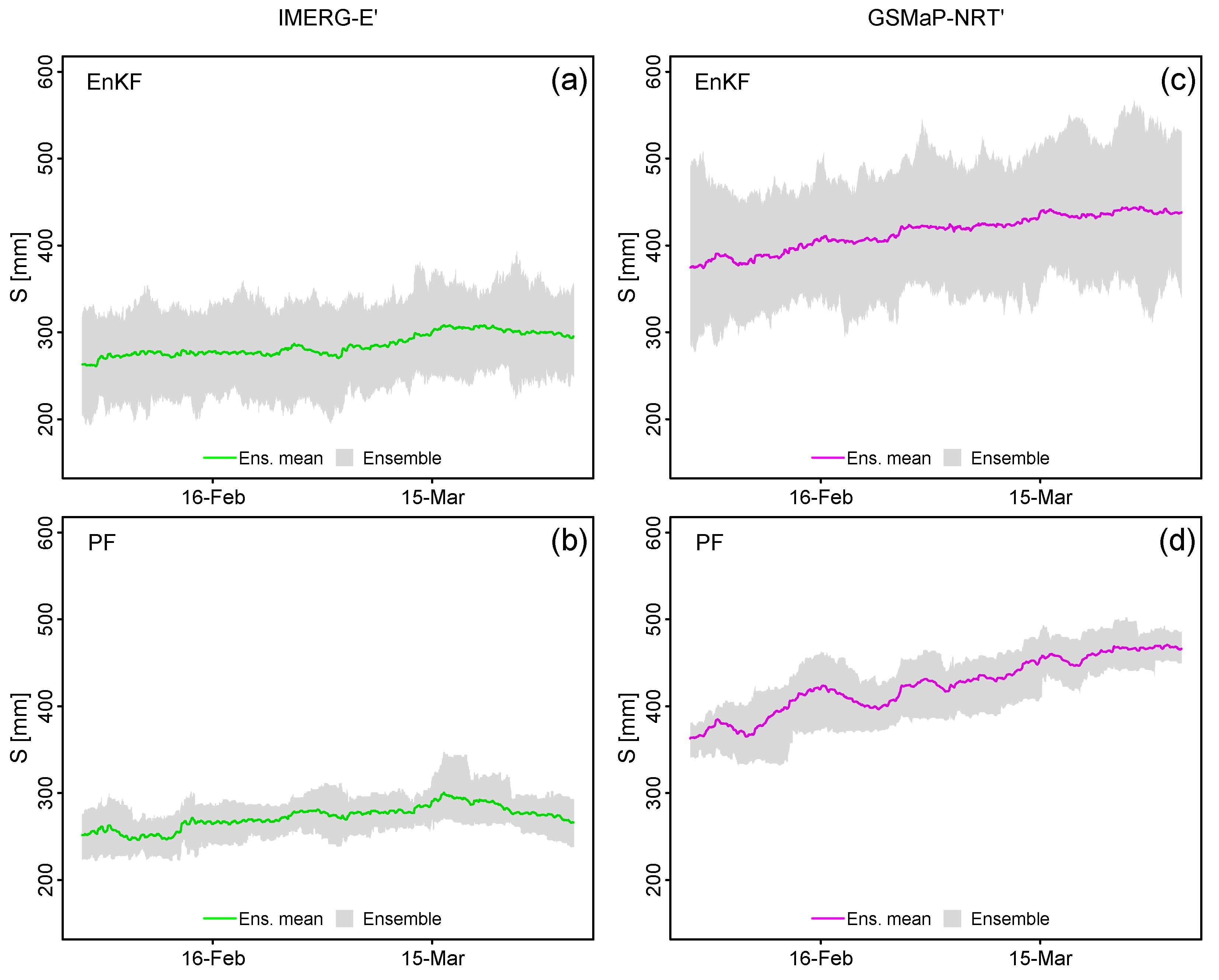
Uncertainties in the state variable S from the production reservoir, as a proxy of Soil Moisture (SM), are illustrated in
Figure 7. Ensemble means is present as green (magenta) for IMERG-E’ (GSMaP-NRT’) driven experiment, and ensemble spreads are shown as gray bounds. Results display huge differences in the SM behavior in all schemes. For instance, SM varies from a minimum value of 192 mm (IMERG-E’+PF,
Figure 7b) to a maximum value of 545 mm (GSMaP-NRT’+EnKF,
Figure 7c).
Overall, SM is higher in GSMA-NRT’ driven experiments than IMERG-E’. Furthermore, similar to streamflow results shown in
Figure 6d-g, uncertainty bounds are wider in EnKF schemes than in PF, independent of the forcing source used. Also, in all cases, ensemble means in
Figure 7 tend to increase from February to March, with a higher SM rate in GSMaP-NRT’ experiments (
Figure 7c-d).
3.3. Forecasting Performance Assessment
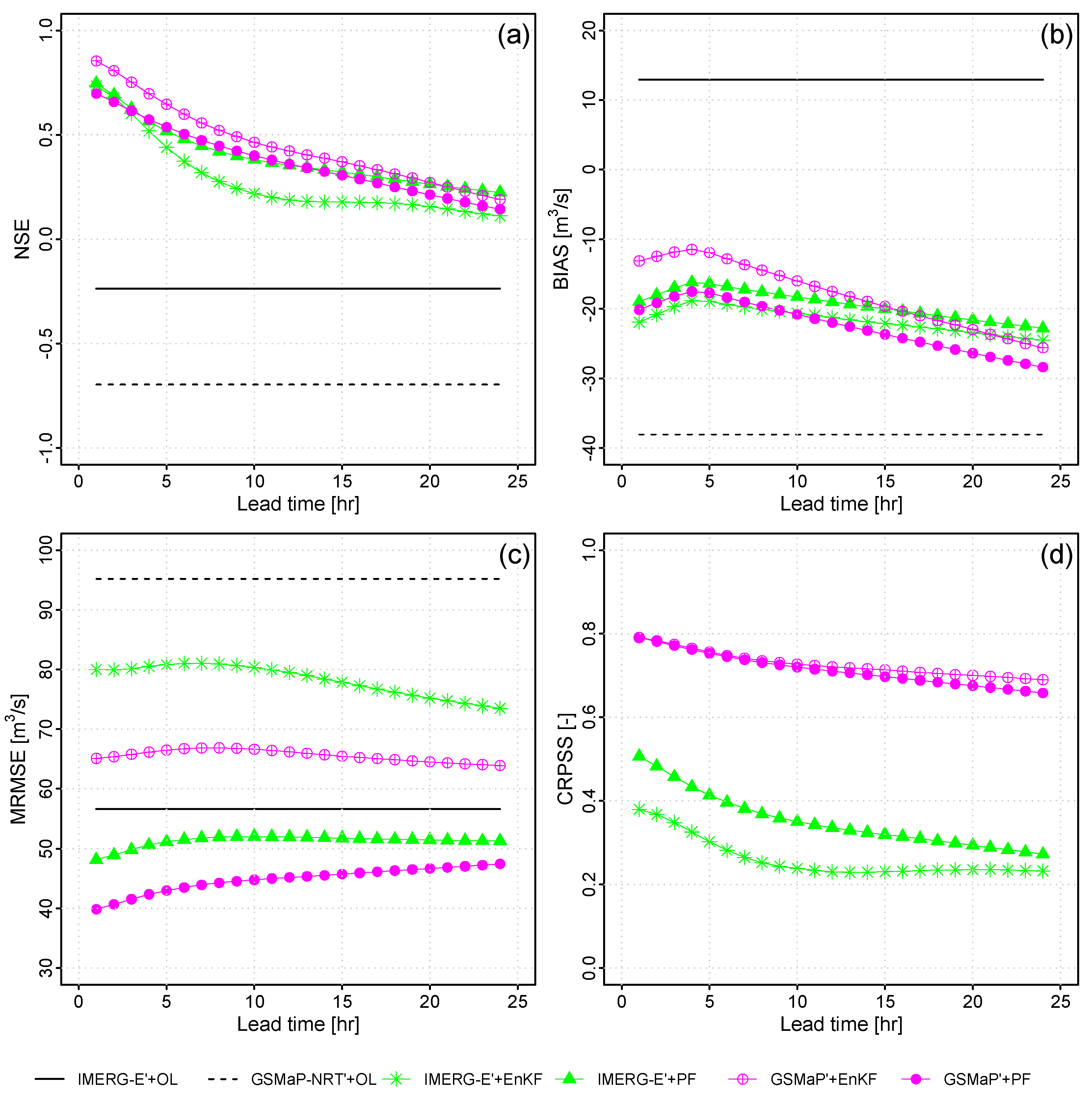
Figure 8 illustrates the forecasting performance after streamflow data assimilation for the lumped hydrological system in the Vilcanota River basin at Pisac stream gauge station using the conceptual GR4H model forced with IMERG-E’ and GSMaP-NRT’.
Initially,
Figure 8a-b shows performance skills for ensemble means flow predictions. In terms of the NSE, the GSMaP-NRT’+EnKF setup has the best performance. NSE values are higher than 0.50 during the first 8 hours, while the remaining schemes exceed this threshold just in the first 5 hours. Furthermore, NSE values in this experiment are always higher than the other ones. Note here that Open Loop models have lower values (NSE < 0) and improve drastically with the application of streamflow DA. Concerning BIAS, negative values are found in all cases, except for the Open Loop model in IMERG-E’, suggesting that forecasted discharges underestimate observations. Also, is observed that negative BIAS values decrease (see the increasing pattern in the plot) during the first 4 hours of forecast and then increase until the 24 hours (decreasing pattern). This increment of negative BIAS is more notable in GSMaP-NRT’ experiments compared to IMERG-E’ ones.
On the other hand, GSMaP-NRT’+PF experiment seems to have a better performance than GSMaP-NRT’+EnKF for ensemble forecast skills present in
Figure 8c-d. For example, the PF performs better than the EnKF algorithm in terms of the MRMSE, specifically in the GSMaP-NRT’-PF scheme. As was expected, MRMSE is worse when increasing lead times from 1 to 24 hours. Furthermore, similar to BIAS, inflection points are observed at 7-8 hours. In the case of the CRPSS, values decrease slowly, especially after 9 - 10 hours. CRPSS values of GSMaP-NRT’ experiments are higher (0.65 – 0.80) than IMERG-E’ schemes (0.21 – 0.54).
In general, forecast skills are worse when lead times rise from 1 to 24 hours at the Pisac gauge station. Also, results demonstrate the benefits of streamflow DA applications compared to Open Loop models. Here we found that GSMaP-NRT’+EnKF setup performs better than the other schemes when evaluating the ensemble means predictions (NSE and BIAS). However, GSMaP-NRT’+PF has the best performance in ensemble evaluation (MRSME and CRPS) due to ensemble spreads having thin uncertainty bounds for PF experiments.
According to the previous assessment of forecast skills in
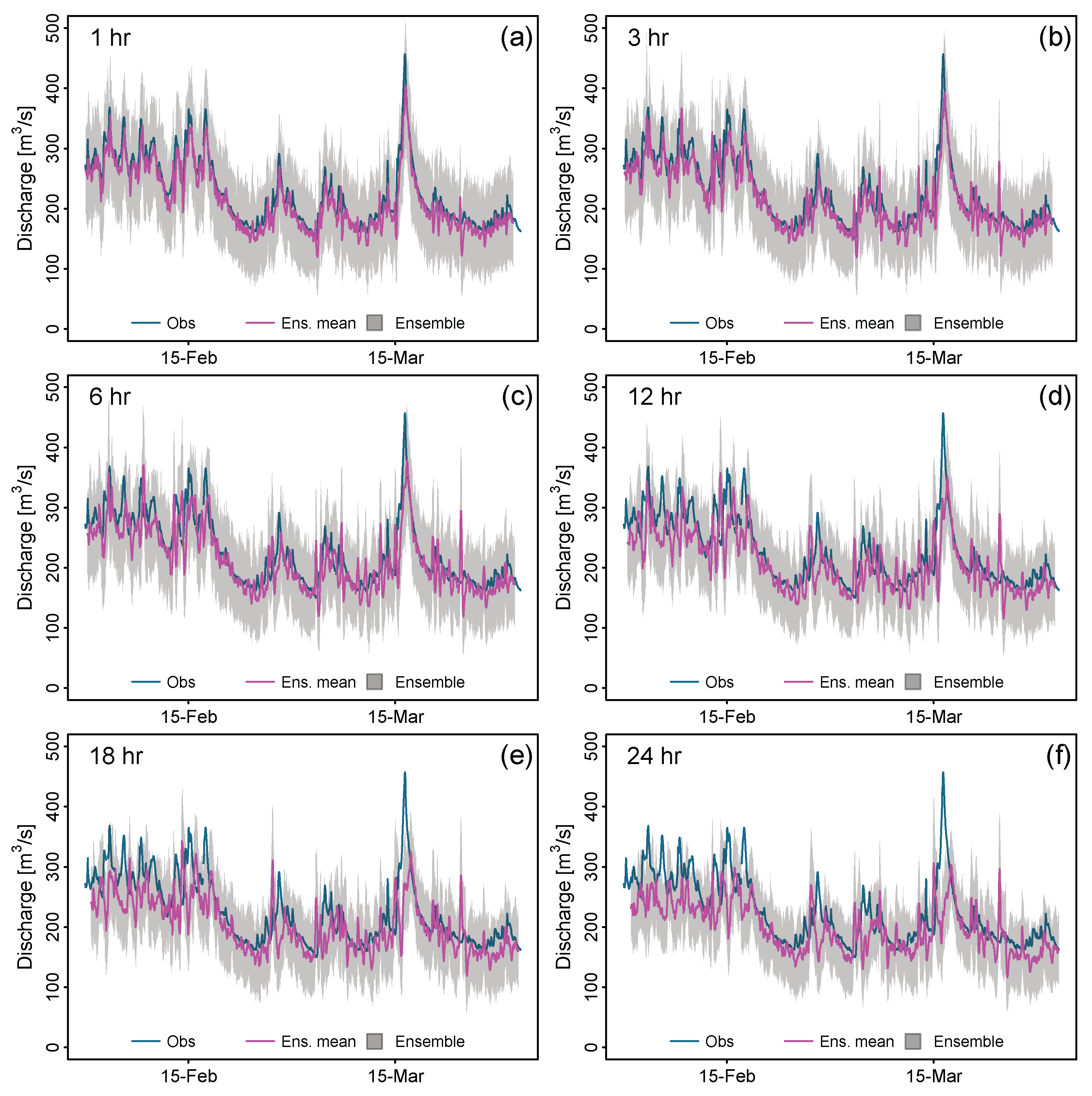
Figure 8, we select the GSMaP-NRT’+EnKF experiment to illustrate the contrast of observed and forecasted discharge times series during February and March 2022 at the Pisac stream gauge station.
Figure 9 displays the comparison between observed (blue lines) and forecasted (magenta lines) hydrographs for lead times of 1, 3, 6, 12, 18, and 24 hours. Also, ensemble spreads from an ensemble size of 100 members are shown as gray bands.
As was noted in the figures, the forecasted discharges are continuously below the observed values. Moreover, this difference increases from lead times of 1 to 24 hours. Thus, as shown in
Figure 8, the forecast accuracy decreases when increasing lead times. Also, peak flows seem to be well represented until the lead time of 6 hours to then being subestimated from 12 hours in advance. For example, the peak flow values during the middle of March 2022 for lead times of 18 (328 m
3/s) and 24 (302 m
3/s) hours hugely subestimate the observed value (465 m
3/s) at the Pisac gauge station.
Overall, the forecasting performance assessment examines skills for the ensemble means and spreads for lead times from 1 to 24 hours. Results show that GSMaP-NRT’ experiment performs better than IMERG-E’ in a lumped system, and the GSMaP-NRT’+EnKF scheme performs better than the other setups, at least for the first 10 hours of forecast.
4. Discussion
4.1. Limitations and Potential of Streamflow Data Assimilation in the Vilcanota River Basin
The results show the potential to improve sub-daily streamflow forecast in the Vilcanota River basin by assimilating real-time observed discharges at the basin outlet. This work establishes the basis for hydrological streamflow predictions in an Andean basin of Peru. However, some important considerations are shown below:
Ensemble spreads of EnKF experiments tend to be wider than PF ones as is displayed in streamflows (
Figure 6) and soil moisture (
Figure 7) simulations. This suggests that EnKF requires a bigger ensemble size than PF to deal with the same uncertainties’ sources. Here the GR4H model was run forward in time with 100 ensemble members according to similar studies in other domains [
53]. Hence, [
54] suggests that EnKF ensemble size influences streamflow DA and must be at least 500 members due to non-Gaussian forecast, but this process will increase the computational demands on operation systems, especially at sub-daily timesteps and operational models. In contrast, the PF algorithm is more flexible about ensemble size but a very small ensemble (e.g. 20, 40) increases filter degeneracy and reduces the number of successful runs [
55,
56]. Moreover, the PF and EnKF are inherently sequential algorithms that are easy to use in real-time forecasting applications because measurements are processed as they become available [
56]. Recent studies in real-time flood forecasting are also incorporating new sequential DA techniques such as the Ensemble Transform Kalman Filter (ETKF) [
57], the covariance resampling for PF [
55], the disaggregated multi-level factorial hydrologic data assimilation (FHDA) [
58], states updates trough backpropagation and deep learning models [
59] that might be tested in future research.
Also, is well known that the forecast accuracy is sensitive to each source of model uncertainty, which is likely to have a differing impact depending mainly on the choice of modeling error scheme and then on the selected DA algorithm. For modeling input errors we use two rainfall sources at basin scale (IMERG-E’ and GSMaP-NRT’) and a space-time correlation using a uniform distribution, so the random perturbations are provided by a first-order autoregressive model similar to [
57]. In this case, autoregressive models similar to [
59] were built for the rainiest months in 2022 due to the focus on improving the forecast accuracy of recent floods. Hence, the dry season might also be tested in future studies to examine model errors related to the uncertainties in low flow measurements and the contribution of groundwater (baseflow) to the surface runoff such as in [
60]. Also, state perturbations were applied only for the production reservoir (S) related to the basin soil moisture following the methodology of [
59] for DA in the GR4H model, but the remaining model states (R, UH1, and UH2) can also be updated thought EnKF and PF algorithms to assess the impact on hourly simulation such presented in [
60] for the GR4J at a daily time step. In case of system output errors, the state-discharge rating curves at the Pisac stream gauge needs to be continuously adjusted to reduce observed streamflow error such as in [
61], especially for low and high flows where streamflow are usually interpolated and extrapolated, respectively. Recently, a new LiDAR sensor has been installed for monitoring water levels such as in [
62], and will support observational real-time flood monitoring.
Furthermore, we note the limitation of lumped-model uncertainties assessments in a basin with an area of 6900 km
2, especially for the local variability impact on the basin’s hydrology. Hence, we highlight the benefits of streamflow DA, in an Andean basin of Peru, to improve forecast accuracy using real-time discharges at the basin outlet. Future works will assess DA techniques in the semi-distributed Vilcanota systems presented by [
60] to prove if incorporating forcing spatialization, river routing, and soil moisture’s sub-basin spatialization in conceptual models, such as in [
61], is more appropriate for Andean basins with sparse data availability. For instance, [
62] suggests that hydrologic river routing such as the Muskingum method is subject to potentially significant errors from structural and parametric uncertainties.
Finally, there is a pending task for generalize from particular experiments to the whole wide hydrological heterogeneity of the Peruvian Andes [
63]. However, the case of the Vilcanota River basin with the four DA assimilation schemes tested here has distinctive features that can be expected to apply over a range of different basins in the Tropical Andes of Peru, that have the same data-scarcity issue [
64]. Finally, the results presented here benchmark the use of EnKF and PF for real-time streamflow DA in the Peruvian Hydrology.
5. Conclusions
Real-time in situ measurements are increasingly being used to improve the estimations of models via data assimilation (DA) techniques. This study addresses the streamflow DA in the Vilcanota River basin and demonstrates the potential of improving sub-daily streamflow forecast at the Pisac stream gauge station. Two sequential algorithms were applied for assimilating real-time observed discharges during February and March 2022. Four DA experiments were computed in a lumped system using two different rainfall sources and a conceptual rainfall-runoff model. The satellite-based GSMaP-NRT product - merged with pluviometric stations - had the best performance for streamflow DA. Also, the GSMaP-NRT’+EnKF scheme shows the best improvement in forecast accuracy, at least during the first 10 hours of lead time. Future research will examine the benefits of streamflow DA in semi-distributed systems to prove if increasing the spatialization of model forcing and states will increase the forecast accuracy at the basin outlet.
Ongoing research contributes to the mitigation of hydrological hazards and constrain flood forecast uncertainties in the Vilcanota River basin. Moreover, the methodology and results reported here benchmark the application of streamflow DA in basins of the Peruvian Tropical Andes with the same sparse data availability and will support the development of more accurate climate services in Peru. Also, establish the basis for ensemble flood prediction applications instead of classic deterministic forecasts. Finally, this work highlights the necessity to improve hydrometeorological observations for a better understating of rainfall-runoff transformation and streamflow predictions in the Tropical Andes.
Author Contributions
Conceptualization, H.LL. and W.L.; methodology, H.LL.; software, H.LL.; validation, H.LL. and W.L.; formal analysis, H.LL.; investigation, H.LL.; resources, W.L.; data curation, H.LL.; writing—original draft preparation, H.LL.; writing—review and editing, H.LL., W.L., and M.A.; visualization, H.LL.; supervision, W.L.; project administration, M.A.; funding acquisition, M.A. All authors have read and agreed to the published version of the manuscript.
Funding
This research was funded by Practical Action Latin America.
Informed Consent Statement
Informed consent was obtained from all subjects involved in the study.
Data Availability Statement
The data presented in this study will be made available on request.
Conflicts of Interest
The authors declare no conflict of interest.
References
- Poveda, G.; Espinoza, J.C.; Zuluaga, M.D.; Solman, S.A.; Garreaud, R.; van Oevelen, P.J. High Impact Weather Events in the Andes. Front Earth Sci. Chin. 2020, 8. [CrossRef]
- Motschmann, A. Water Resource Risks in the Andes of Peru: An Integrative Perspective, University of Zurich: Zürich, 2021.
- Ávila, Á.; Guerrero, F.C.; Escobar, Y.C.; Justino, F. Recent Precipitation Trends and Floods in the Colombian Andes. Water 2019, 11, 379. [CrossRef]
- Pinos, J.; Orellana, D.; Timbe, L. Assessment of Microscale Economic Flood Losses in Urban and Agricultural Areas: Case Study of the Santa Bárbara River, Ecuador. Nat. Hazards 2020, 103, 2323–2337. [CrossRef]
- Höglund, S.; Rodin, L. Flood Simulation in the Colombian Andean Region Using UAV-Based LiDAR: Minor Field Study in Colombia; diva-portal.org, 2023;
- Muñoz, P.; Orellana-Alvear, J.; Bendix, J.; Feyen, J.; Célleri, R. Flood Early Warning Systems Using Machine Learning Techniques: The Case of the Tomebamba Catchment at the Southern Andes of Ecuador. Hydrology 2021, 8, 183. [CrossRef]
- Wu, W.; Emerton, R.; Duan, Q.; Wood, A.W.; Wetterhall, F.; Robertson, D.E. Ensemble Flood Forecasting: Current Status and Future Opportunities. WIREs Water 2020, 7, e1432. [CrossRef]
- Drenkhan, F.; Carey, M.; Huggel, C.; Seidel, J.; Oré, M.T. The Changing Water Cycle: Climatic and Socioeconomic Drivers of Water-Related Changes in the Andes of Peru. Wiley Interdisciplinary Reviews: Water 2015, 2, 715–733. [CrossRef]
- Huggel, C.; Raissig, A.; Rohrer, M.; Romero, G.; Diaz, A.; Salzmann, N. How Useful and Reliable Are Disaster Databases in the Context of Climate and Global Change? A Comparative Case Study Analysis in Peru. Nat. Hazards Earth Syst. Sci. 2015, 15, 475–485. [CrossRef]
- Espinoza, J.C.; Chavez, S.; Ronchail, J.; Junquas, C.; Takahashi, K.; Lavado, W. Rainfall Hotspots over the Southern Tropical Andes: Spatial Distribution, Rainfall Intensity, and Relations with Large-Scale Atmospheric Circulation. Water Resour. Res. 2015, 51, 3459–3475. [CrossRef]
- Llauca, H.; Leon, K.; Lavado-Casimiro, W. Construction of a Daily Streamflow Dataset for Peru Using a Similarity-Based Regionalization Approach and a Hybrid Hydrological Modeling Framework. Journal of Hydrology: Regional Studies 2023, 47, 101381. [CrossRef]
- Lavado-Casimiro, W.; Silvestre, E.; Pulache, W. Extreme Rainfall Trends around Cusco and Its Relationship with the Floods in January 2010. Revista Peruana Geo-Atmosferica 2010.
- Waldo, L.-C.; Juan Carlos, J.; Harold, L.; Karen, L.; Clara, O.; Alan, L.; Adrian, H.; Oscar, F.; Julia, A.; Pedro, R.; et al. ANDES: The First System for Flash Flood Monitoring and Forecasting in Peru.; ui.adsabs.harvard.edu, May 1, 2020; p. 3759.
- Fan, Y. Uncertainty Quantification in Hydrologic Predictions: A Brief Review. J. Environ. Inform. Lett 2019. [CrossRef]
- Gupta, A.; Govindaraju, R.S. Uncertainty Quantification in Watershed Hydrology: Which Method to Use? J. Hydrol. 2023, 616, 128749. [CrossRef]
- Moges, E.; Demissie, Y.; Larsen, L.; Yassin, F. Review: Sources of Hydrological Model Uncertainties and Advances in Their Analysis. Water 2020, 13, 28. [CrossRef]
- Levin, S.B.; Briggs, M.A.; Foks, S.S.; Goodling, P.J.; Raffensperger, J.P.; Rosenberry, D.O.; Scholl, M.A.; Tiedeman, C.R.; Webb, R.M. Uncertainties in Measuring and Estimating Water-budget Components: Current State of the Science. WIREs Water 2023. [CrossRef]
- Segovia-Cardozo, D.A.; Bernal-Basurco, C.; Rodríguez-Sinobas, L. Tipping Bucket Rain Gauges in Hydrological Research: Summary on Measurement Uncertainties, Calibration, and Error Reduction Strategies. Sensors 2023, 23, 5385. [CrossRef]
- McMillan, H.K.; Westerberg, I.K.; Krueger, T. Hydrological Data Uncertainty and Its Implications. WIREs Water 2018, 5, e1319. [CrossRef]
- Saavedra, D.; Mendoza, P.A.; Addor, N.; Llauca, H.; Vargas, X. A Multi-objective Approach to Select Hydrological Models and Constrain Structural Uncertainties for Climate Impact Assessments. Hydrol. Process. 2021. [CrossRef]
- Herrera, P.A.; Marazuela, M.A.; Hofmann, T. Parameter Estimation and Uncertainty Analysis in Hydrological Modeling. WIREs Water 2022, 9. [CrossRef]
- Panchanathan, A.; Ahrari, A.H.; Ghag, K.; Mustafa, S.M.T.; Haghighi, A.T.; Kløve, B.; Oussalah, M. An Overview of Approaches for Reducing Uncertainties in Hydrological Forecasting: Progress, and Challenges 2023.
- Rasmussen, J.; Madsen, H.; Jensen, K.H.; Refsgaard, J.C. Data Assimilation in Integrated Hydrological Modelling in the Presence of Observation Bias. Hydrol. Earth Syst. Sci. Discuss. 2015, 12, 8131–8173. [CrossRef]
- Avellaneda, P.M.; Ficklin, D.L.; Lowry, C.S.; Knouft, J.H.; Hall, D.M. Improving Hydrological Models with the Assimilation of Crowdsourced Data. Water Resour. Res. 2020, 56. [CrossRef]
- Boucher, M.-A.; Quilty, J.; Adamowski, J. Data Assimilation for Streamflow Forecasting Using Extreme Learning Machines and Multilayer Perceptrons. Water Resour. Res. 2020, 56, e2019WR026226. [CrossRef]
- Noh, S.J.; Lee, H.S.; Seo, D.J. Streamflow Data Assimilation for Hydrologic River Routing: Advances and Challenges.; ui.adsabs.harvard.edu, December 1 2019; Vol. 2019, pp. H31J-1853.
- Mazzoleni, M.; Noh, S.J.; Lee, H.; Liu, Y.; Seo, D.-J.; Amaranto, A.; Alfonso, L.; Solomatine, D.P. Real-Time Assimilation of Streamflow Observations into a Hydrological Routing Model: Effects of Model Structures and Updating Methods. Hydrol. Sci. J. 2018, 63, 386–407. [CrossRef]
- Li, Y.; Ryu, D.; Western, A.W.; Wang, Q.J. Assimilation of Stream Discharge for Flood Forecasting: Updating a Semidistributed Model with an Integrated Data Assimilation Scheme. Water Resour. Res. 2015, 51, 3238–3258. [CrossRef]
- Nayak, A.K.; Biswal, B.; Sudheer, K.P. Role of Hydrological Model Structure in the Assimilation of Soil Moisture for Streamflow Prediction. J. Hydrol. 2021, 598, 126465. [CrossRef]
- Alvarado-Montero, R.; Uysal, G.; Collados-Lara, A.-J.; Arda Şorman, A.; Pulido-Velazquez, D.; Şensoy, A. Comparison of Sequential and Variational Assimilation Methods to Improve Hydrological Predictions in Snow Dominated Mountainous Catchments. J. Hydrol. 2022, 612, 127981. [CrossRef]
- Clark, M.P.; Rupp, D.E.; Woods, R.A.; Zheng, X.; Ibbitt, R.P.; Slater, A.G.; Schmidt, J.; Uddstrom, M.J. Hydrological Data Assimilation with the Ensemble Kalman Filter: Use of Streamflow Observations to Update States in a Distributed Hydrological Model. Adv. Water Resour. 2008, 31, 1309–1324. [CrossRef]
- Li, Y.; Ryu, D.; Western, A.W.; Wang, Q.J.; Robertson, D.E.; Crow, W.T. An Integrated Error Parameter Estimation and Lag-Aware Data Assimilation Scheme for Real-Time Flood Forecasting. J. Hydrol. 2014, 519, 2722–2736. [CrossRef]
- Pathiraja, S.; Moradkhani, H.; Marshall, L.; Sharma, A.; Geenens, G. Data-driven Model Uncertainty Estimation in Hydrologic Data Assimilation. Water Resour. Res. 2018, 54, 1252–1280. [CrossRef]
- Bergeron, J.; Leconte, R.; Trudel, M.; Farhoodi, S. On the Choice of Metric to Calibrate Time-Invariant Ensemble Kalman Filter Hyper-Parameters for Discharge Data Assimilation and Its Impact on Discharge Forecast Modelling. Hydrology 2021, 8, 36. [CrossRef]
- Piazzi, G.; Thirel, G.; Perrin, C.; Delaigue, O. Sequential Data Assimilation for Streamflow Forecasting: Assessing the Sensitivity to Uncertainties and Updated Variables of a Conceptual Hydrological Model at Basin Scale. Water Resour. Res. 2021, 57. [CrossRef]
- Leach, J.M.; Coulibaly, P. An Extension of Data Assimilation into the Short-Term Hydrologic Forecast for Improved Prediction Reliability. Adv. Water Resour. 2019, 134, 103443. [CrossRef]
- Wang, S.; Ancell, B.C.; Huang, G.H.; Baetz, B.W. Improving Robustness of Hydrologic Ensemble Predictions through Probabilistic Pre- and Post-processing in Sequential Data Assimilation. Water Resour. Res. 2018, 54, 2129–2151. [CrossRef]
- Muñoz-Castro, E.; Mendoza, P.A.; Vargas, X. The Role of Parameter Estimation Strategies on Ensemble Streamflow Prediction Results across Extratropical Andean Catchments.; ui.adsabs.harvard.edu, May 1 2020; p. 10845.
- Mendoza, P.A.; McPhee, J.; Vargas, X. Uncertainty in Flood Forecasting: A Distributed Modeling Approach in a Sparse Data Catchment. Water Resour. Res. 2012, 48. [CrossRef]
- Cortés, G.; Girotto, M.; Margulis, S. Snow Process Estimation over the Extratropical Andes Using a Data Assimilation Framework Integrating MERRA Data and Landsat Imagery. Water Resour. Res. 2016, 52, 2582–2600. [CrossRef]
- Emery, C.M.; Biancamaria, S.; Boone, A.; Ricci, S.; Rochoux, M.C.; Pedinotti, V.; David, C.H. Assimilation of Wide-Swath Altimetry Water Elevation Anomalies to Correct Large-Scale River Routing Model Parameters. Hydrol. Earth Syst. Sci. 2020, 24, 2207–2233. [CrossRef]
- Wongchuig, S.C.; de Paiva, R.C.D.; Siqueira, V.; Collischonn, W. Hydrological Reanalysis across the 20th Century: A Case Study of the Amazon Basin. J. Hydrol. 2019, 570, 755–773. [CrossRef]
- Paiva, R.C.D.; Collischonn, W.; Bonnet, M.-P.; de Gonçalves, L.G.G.; Calmant, S.; Getirana, A.; Santos da Silva, J. Assimilating in Situ and Radar Altimetry Data into a Large-Scale Hydrologic-Hydrodynamic Model for Streamflow Forecast in the Amazon. Hydrol. Earth Syst. Sci. Discuss. 2013, 10, 2879–2925. [CrossRef]
- Durand, M.; Andreadis, K.M.; Alsdorf, D.E. Estimation of Bathymetric Depth and Slope from Data Assimilation of Swath Altimetry into a Hydrodynamic Model. Geophysical 2008. [CrossRef]
- Llauca, H.; Lavado-Casimiro, W.; León, K.; Jimenez, J.; Traverso, K.; Rau, P. Assessing Near Real-Time Satellite Precipitation Products for Flood Simulations at Sub-Daily Scales in a Sparsely Gauged Watershed in Peruvian Andes. Remote Sensing 2021, 13, 826. [CrossRef]
- Fernandez-Palomino, C.A.; Hattermann, F.F.; Krysanova, V.; Vega-Jácome, F.; Bronstert, A. Towards a More Consistent Eco-Hydrological Modelling through Multi-Objective Calibration: A Case Study in the Andean Vilcanota River Basin, Peru. Hydrol. Sci. J. 2021, 66, 59–74. [CrossRef]
- Huerta, A.; Bonnesoeur, V.; Cuadros-Adriazola, J.; Gutierrez, L.; Ochoa-Tocachi, B.F.; Román-Dañobeytia, F.; Lavado-Casimiro, W. PISCOeo_pm, a Reference Evapotranspiration Gridded Database Based on FAO Penman-Monteith in Peru. Scientific Data 2022, 9, 1–18. [CrossRef]
- Moine, N. Le Bassin Versant de Surface vu Par Le Souterrain: Une Voie d’amélioration Des Performances et Du Réalisme Des Modèles Pluie-Débit? Ph.D. Thesis, Université Pierre et Marie, 2008.
- Perrin, C.; Michel, C.; Andréassian, V. Improvement of a Parsimonious Model for Streamflow Simulation. J. Hydrol. 2003, 279, 275–289. [CrossRef]
- Duan, Q.Y.; Gupta, V.K.; Sorooshian, S. Shuffled Complex Evolution Approach for Effective and Efficient Global Minimization. J. Optim. Theory Appl. 1993, 76, 501–521. [CrossRef]
- Jafarzadegan, K.; Abbaszadeh, P.; Moradkhani, H. Sequential Data Assimilation for Real-Time Probabilistic Flood Inundation Mapping. Hydrol. Earth Syst. Sci. 2021, 25, 4995–5011. [CrossRef]
- Piazzi, G.; Delaigue, O. Ensemble-Based Data Assimilation with GR Hydrological Models (v. 0.1.3). HAL 2021, doi:hal-03301603.
- Moradkhani, H.; Sorooshian, S.; Gupta, H.V.; Houser, P.R. Dual State–Parameter Estimation of Hydrological Models Using Ensemble Kalman Filter. Adv. Water Resour. 2005, 28, 135–147. [CrossRef]
- Reichle, R.H.; McLaughlin, D.B.; Entekhabi, D. Hydrologic Data Assimilation with the Ensemble Kalman Filter. Mon. Weather Rev. 2002, 130, 103–114. [CrossRef]
- Berg, D.; Bauser, H.H.; Roth, K. Covariance Resampling for Particle Filter – State and Parameter Estimation for Soil Hydrology. Hydrol. Earth Syst. Sci. 2019, 23, 1163–1178. [CrossRef]
- Jamal, A.; Linker, R. Covariance-Based Selection of Parameters for Particle Filter Data Assimilation in Soil Hydrology. Water 2022, 14, 3606. [CrossRef]
- He, X.; Lucatero, D.; Ridler, M.-E.; Madsen, H.; Kidmose, J.; Hole, Ø.; Petersen, C.; Zheng, C.; Refsgaard, J.C. Real-Time Simulation of Surface Water and Groundwater with Data Assimilation. Adv. Water Resour. 2019, 127, 13–25. [CrossRef]
- Wang, F.; Huang, G.H.; Fan, Y.; Li, Y.P. Development of a Disaggregated Multi-Level Factorial Hydrologic Data Assimilation Model. J. Hydrol. 2022, 610, 127802. [CrossRef]
- Nearing, G.S.; Klotz, D.; Frame, J.M. Data Assimilation and Autoregression for Using Near-Real-Time Streamflow Observations in Long Short-Term Memory Networks. Hydrol. Earth Syst. Sci. 2022. [CrossRef]
- De Sousa, E.R.; Hipsey, M.R.; Vogwill, R.I.J. Data Assimilation, Sensitivity Analysis and Uncertainty Quantification in Semi-Arid Terminal Catchments Subject to Long-Term Rainfall Decline. Front Earth Sci. Chin. 2023, 10. [CrossRef]
- Mansanarez, V.; Renard, B.; Coz, J.L. Shift Happens! Adjusting Stage-discharge Rating Curves to Morphological Changes at Known Times. Water Resources Research 2019. [CrossRef]
- Paul, J.D.; Buytaert, W.; Sah, N. A Technical Evaluation of Lidar-based Measurement of River Water Levels. Water Resour. Res. 2020, 56, e2019WR026810. [CrossRef]
- Llauca, H.; Lavado-Casimiro, W.; Montesinos, C.; Santini, W.; Rau, P. PISCO_HyM_GR2M: A Model of Monthly Water Balance in Peru (1981–2020). Water 2021. [CrossRef]
- Condom, T.; Martínez, R.; Pabón, J.D.; Costa, F.; Pineda, L.; Nieto, J.J.; López, F.; Villacis, M. Climatological and Hydrological Observations for the South American Andes: In Situ Stations, Satellite, and Reanalysis Data Sets. Front Earth Sci. Chin. 2020, 8. [CrossRef]
Figure 1.
The Vilcanota river basin at Pisac gauge station located in the southern Peruvian Tropical Andes. The available pluviometric network in the study domain is shown as orange triangles.
Figure 1.
The Vilcanota river basin at Pisac gauge station located in the southern Peruvian Tropical Andes. The available pluviometric network in the study domain is shown as orange triangles.
Figure 2.
Seasonal variation (1981 — 2010) of mean areal precipitation, monthly streamflows, and mean air temperature in the Vilcanota River basin at Pisac stream gauge station.
Figure 2.
Seasonal variation (1981 — 2010) of mean areal precipitation, monthly streamflows, and mean air temperature in the Vilcanota River basin at Pisac stream gauge station.
Figure 3.
Structure of the parsimonious GR4H model [
32].
Figure 3.
Structure of the parsimonious GR4H model [
32].
Figure 4.
Streamflow Data Assimilation framework in the Vilcanota River basin.
Figure 4.
Streamflow Data Assimilation framework in the Vilcanota River basin.
Figure 5.
(a-b) Comparison of simulated (IMERG-E’ and GSMaP-NRT’) and observed hourly flow series at Pisac stream gauge station during 2017 - 2022. The Red dashed box represents the rainiest months in 2022. (c-d) Scatter plots between observed and simulated discharges for the rainiest months in 2022.
Figure 6.
Comparison between observed and simulated hourly flow series during February and March 2022 at the Pisac stream gauge station for (a) IMERG-E’+EnKF, (b) IMERG-E’+KF, (c) GSMaP-NRT’+EnKF, and (d) GSMaP-NRT’+PF experiments.
Figure 6.
Comparison between observed and simulated hourly flow series during February and March 2022 at the Pisac stream gauge station for (a) IMERG-E’+EnKF, (b) IMERG-E’+KF, (c) GSMaP-NRT’+EnKF, and (d) GSMaP-NRT’+PF experiments.
Figure 7.
Uncertainty in simulated soil moisture (S) from GR4H model in the Vilcanota basin during February and March 2022 for (a) IMERG-E’+EnKF, (b) IMERG-E’+KF, (c) GSMaP-NRT’+EnKF, and (d) GSMaP-NRT’+PF experiments.
Figure 7.
Uncertainty in simulated soil moisture (S) from GR4H model in the Vilcanota basin during February and March 2022 for (a) IMERG-E’+EnKF, (b) IMERG-E’+KF, (c) GSMaP-NRT’+EnKF, and (d) GSMaP-NRT’+PF experiments.
Figure 8.
Performance skills of hourly forecasted discharges from 1 to 24 hours of lead times at Pisac stream gauge station from February to March 2022.
Figure 8.
Performance skills of hourly forecasted discharges from 1 to 24 hours of lead times at Pisac stream gauge station from February to March 2022.
Figure 9.
Comparison of observed and forecasted hourly flow series at Pisac station from February to March 2023, for lead times of 1, 3, 6, 12, 18, and 24 hours in the GSMaP-NRT’+EnKF experiment.
Figure 9.
Comparison of observed and forecasted hourly flow series at Pisac station from February to March 2023, for lead times of 1, 3, 6, 12, 18, and 24 hours in the GSMaP-NRT’+EnKF experiment.
Table 1.
Selected gauges with hourly records in the study domain.
Table 1.
Selected gauges with hourly records in the study domain.
| Type |
Station |
Abrev. |
Longitude [ºW] |
Latitude [ºS] |
Elevation [m.a.s.l.] |
| Fluviometric |
Pisac |
PIS |
71.84 |
13.43 |
2791.65 |
| Pluviometric |
Acjanaco Gore |
AGR |
71.62 |
13.20 |
3466.11 |
| Calca |
CAL |
71.96 |
13.33 |
2921.24 |
| Casaccancha |
CAS |
72.30 |
13.99 |
4033.16 |
| Huayllabamba |
HUA |
72.45 |
13.27 |
2976.55 |
| Intihuatana M |
INM |
72.56 |
13.17 |
1778.23 |
| Machupicchu |
MAC |
72.55 |
13.18 |
2399.80 |
| Marcapata Gore |
MAR |
70.90 |
13.50 |
1792.76 |
| Qorihuayrachina |
QOR |
72.43 |
13.22 |
2517.25 |
| Salcca |
SAL |
71.23 |
14.17 |
3920.10 |
| San Pablo |
SPB |
72.62 |
13.03 |
1228.11 |
| Santo Tomas |
STM |
72.10 |
14.45 |
3665.48 |
| Sicuani |
SIC |
71.24 |
14.24 |
3534.95 |
Table 2.
Statistical metrics and their corresponding equations used for evaluating the hydrological performance of the GR4H model.
Table 2.
Statistical metrics and their corresponding equations used for evaluating the hydrological performance of the GR4H model.
| Statistical Metric |
Equation |
Min, Max, Optimal |
Emphasis |
Logarithmic Nash-Sutcliffe Efficiency
(logNSE)
[-] |
|
-∞,1,1 |
Low flows |
Nash-Sutcliffe Efficiency with Box-Cox transformation
(BoxNSE)
[-] |
|
-∞,1,1 |
Middle flows |
Kling-Gupta Efficiency
(KGE)
[-] |
|
-∞,1,1 |
Variance and high flows. |
Bias
(BIAS)
[%] |
|
0,+ ∞,0 |
Average trend of simulated flows |
Table 3.
Statistical metrics and their respective equation used for evaluating forecasts.
Table 3.
Statistical metrics and their respective equation used for evaluating forecasts.
| Statistical Metric |
Equation |
Nash-Sutcliffe
Efficiency
(NSE)
[-] |
|
Bias (BIAS)
[m3/s] |
|
Mean of Ensemble Root Mean Squared
Error
(MRMSE)
[m3/s] |
|
Continuous Ranked Probability Skill Score (CRPSS)
[-] |
|
Table 4.
Model performance metrics during calibration and validation periods.
Table 4.
Model performance metrics during calibration and validation periods.
| Statistic Metric |
Calibration |
Validation |
| IMERG-E' |
GSMaP-NRT' |
IMERG-E' |
GSMaP-NRT' |
| logNSE |
0.875 |
0.792 |
0.878 |
0.786 |
| BoxNSE |
0.883 |
0.831 |
0.878 |
0.819 |
| KGE |
0.912 |
0.871 |
0.869 |
0.789 |
| BIAS |
0.003 |
0.003 |
0.016 |
0.029 |
|
Disclaimer/Publisher’s Note: The statements, opinions and data contained in all publications are solely those of the individual author(s) and contributor(s) and not of MDPI and/or the editor(s). MDPI and/or the editor(s) disclaim responsibility for any injury to people or property resulting from any ideas, methods, instructions or products referred to in the content. |
© 2023 by the authors. Licensee MDPI, Basel, Switzerland. This article is an open access article distributed under the terms and conditions of the Creative Commons Attribution (CC BY) license (http://creativecommons.org/licenses/by/4.0/).
