A Transfer Learning-Based Deep Convolutional Neural Network for Detection of Fusarium Wilt in Banana Crops

1. Introduction

Banana (Musa spp.) is one of the most widely produced cash crops in the tropical regions of the world and the fourth most important crop among developing nations. Over 130 countries export bananas, contributing to a total revenue of 50 billion dollars in revenue per year(Ploetz, 2021). Fusarium wilt or Panama disease is caused by the Fusarium oxysporum f. sp. cubense tropical race 4 (TR4), is a well-known threat to global banana production (Heslop-Harrison, Schwarzacher, 2007; Shen et al., 2019). TR4 infected hundreds of thousands of hectares of banana plantations throughout countries like China, India, the Philippines, Australia, and Mozambique (Ordonez et al., 2015).

Four to five weeks after inoculation with Foc, banana crops begin to exhibit the main symptom of Fusarium wilt, yellowing of their leaves. TR4 can spread through flowing water, farm equipment, infected plant material, and soil contamination. Approximately four to five weeks after being inoculated with TR4, banana crops start displaying the primary symptom of Fusarium wilt: the yellowing of their leaves. These once-vibrant leaves gradually begin to droop and eventually collapse, forming a ring of lifeless foliage encircling the pseudo-stem of the crop (Van Den Berg et al., 2007). Over time, an increasing number of leaves experience wilting and collapse, resulting in the entire canopy of the crop being composed solely of withering and deceased leaves.

Currently, the main method used to manage Fusarium wilt is to inspect banana plantations with manual labor in hopes to identify these yellowing leaves. However, this process requires enormous amounts of time and money to perform (Ye et al., 2020). Also, manual inspection quality is affected by the experience and expertise of the farmer performing the inspection, meaning accuracy of diagnosis cannot be ensured (Mahlein, 2016). Additionally,there are currently no chemical or physical treatments available that can effectively control Fusarium Wilt. Once the signs of this disease are identified, the only viable treatment option is the rapid removal of the crop in order to prevent a large-scale infection from occurring (Lin et al., 2017).

Alternatively, Remote sensing has been used in recent studies to detect the presence of Fusarium wilt. For example, a DJI Phantom 4 quad copter (DJI Innovations, Shenzhen, China) equipped with a MicaSense RedEdge M^TM five-band multi spectral camera to perform remote sensing surveys of banana plantations in China (Ye et al., 2020). The multi spectral images was then used to calculate different vegetation indices, attempting to find the infection status of Fusarium wilt in the plantation. The same approach used in (Zhang et al., 2022) to detect Fusarium wilt on banana plantations.

The main drawback to these remote sensing detection systems, despite their ability to detect Panama disease, is similar to that of conducting manual inspections: the high cost. The high-quality multispectral and hyperspectral cameras required by these types of detection systems can range in cost from several thousands of dollars to tens of thousands of dollars. Given that Fusarium wilt infections mostly occur in developing countries on the continents of South America, Africa, and South Asia (Dita et al., 2018), it is clear that farmers in those regions cannot afford high quality spectral cameras and the computational power used to analyze spectral images.

Presently, convolutional neural networks have been used to detect many different plant diseases through their symptoms within the visible light spectrum. In computer vision, deep convolutional neural networks (CNNs) can achieve excellent performance in image classification tasks (Mukti and Biswas, 2019). CNNs are a variant of deep neural networks that are designed to mimic the cognitive process of human vision. CNNs receive an input, usually in the form of an image, which is then fed through layers of neurons that perform nonlinear operations, lastly, the output is in the form of a list of scores between 0 and 1, each of which represents the likelihood of the image belonging to an image class. The nonlinear operations at these neurons are optimized through a training procedure (O’Shea and Nash, 2015).

Transfer learning is a technique used in the design of deep learning models to reduce the need for large training datasets and high computational cost for training. Transfer learning essentially works by integrating the knowledge of a previously trained CNN model into a new CNN model desgined for a specific task(Shaha and Pawar, 2018). Transfer learning approaches have been used in plant classification, sentiment classification, software defect prediction and more (Geetharamani and Pandian, 2019). There are several pre-trained models that can be selected as the base model for transfer learning, such as ResNet, AlexNet, Inception V-3, VGG16, and ImageNet. In (Mutki and Biswas, 2019) the authors evaluated the aforementioned four pre-trained models in a transfer learning based plant disease detection task. It was found that ResNet-50 is the best model and achieves an accuracy of 0.9980.

1.1. Literature Review

CNNs have been used to detect some plant diseases, such as soybean plant diseases (Wallelign et al., 2018), apple black rot, grape leaf blight, tomato leaf mold, cherry powdery mildew, potato with early blight, and bacterial spots on a peach (Geetharamani and Pandian, 2019). In (Pandian et al., 2022), the authors were able to create a convolutional neural network model for detecting 58 classes of plant leaves from aloe vera, apple, banana, cherry, citrus, corn, coffee, grape, paddy, peach, pepper, strawberry, tea, tomato, and wheat crops.

In (Sangeetha et al., 2023), the authors developed a deep learning based neural network model to identify Fusarium wilt. They were able to achieve an accuracy of 0.9156 after evaluation of their model on 700 samples of diseased and healthy banana leaf images. The accuracy achieved in their study was around 0.065 lower than the 0.98 accuracy obtained in this paper. Their samples included completely healthy, partially affected, and fully affected banana crop images.

As previously mentioned, (Ye et al., 2020) proposed a remote sensing-based detection model of fusarium wilt on banana plantations in China. Their model leveraged the changes to the vegetation indices caused by fusarium wilt to detect the disease.

In (Ibarra et al., 2023), the authors utilized the Yolo v4 neural network model embedded in a Raspberry Pi to detect fusarium wilt in banana leaves. The system consisted of a power source connected to a Raspberry Pi displayed on a small LCD screen. Their handheld system was able to identify the infection with an accuracy of 0.90 in the field. Additionally, their system is much more compact and portable than existing options and less reliant on internet and computational power than smartphone apps. The Yolo framework essentially takes one shot of the identification target and makes a rapid prediction using a reasonable amount of computational power, sacrificing accuracy for quickness.

In (Chaudhari and Patil, 2020), the authors proposed the use of a Support Vector Machine (SVM) classification framework to identify four types of banana diseases in India. These four were sigatoka, cmv, bacterial wilt and Fusarium Wilt. Their classification performed with an average accuracy of around 0.85 in detecting these diseases with accuracies of 0.84, 0.86, 0.85, and 0.85 respectively for the four diseases.

1.2. Objectives

The main objectives of this study were to (I) build and train a transfer learning-based convolutional neural network model for the identification of Fusarium wilt in banana crops, (II) use the ResNet-50 pre-trained model as a base in the neural network, and (III) to assess the precision of this model in identifying Fusarium wilt.

2. Materials and Methods

2.1. Dataset

In (Medhi and Deb, 2022), the authors created a comprehensive data set comprising diverse images of banana diseases and healthy plant samples. The data set used in this study for the purpose of training the CNN model is a subset of their data. The initial data set consisted of approximately 100 images of Fusarium wilt infected banana leaves, as well as 100 images featuring healthy banana leaves. These images were captured at different times of the day, under varying environmental conditions, ensuring a wide range of scenarios for greater model robustness.

The original images from the data set had dimensions of 256 x 256 pixels. However, to align with the dimensions of the input layer in the CNN model, the images needed to be resized. The images were adjusted to a standard size of 224 x 224 pixels. This resizing ensured that all input images were consistent in terms of dimensions, enabling seamless processing within the CNN model.

By adjusting the image dimensions to match the input layer’s size, the CNN model was able to receive and process the image inputs. This harmonization of image sizes enabled a consistent and fair comparison across different samples during the training process, ensuring that the model learned from the entire data set uniformly.

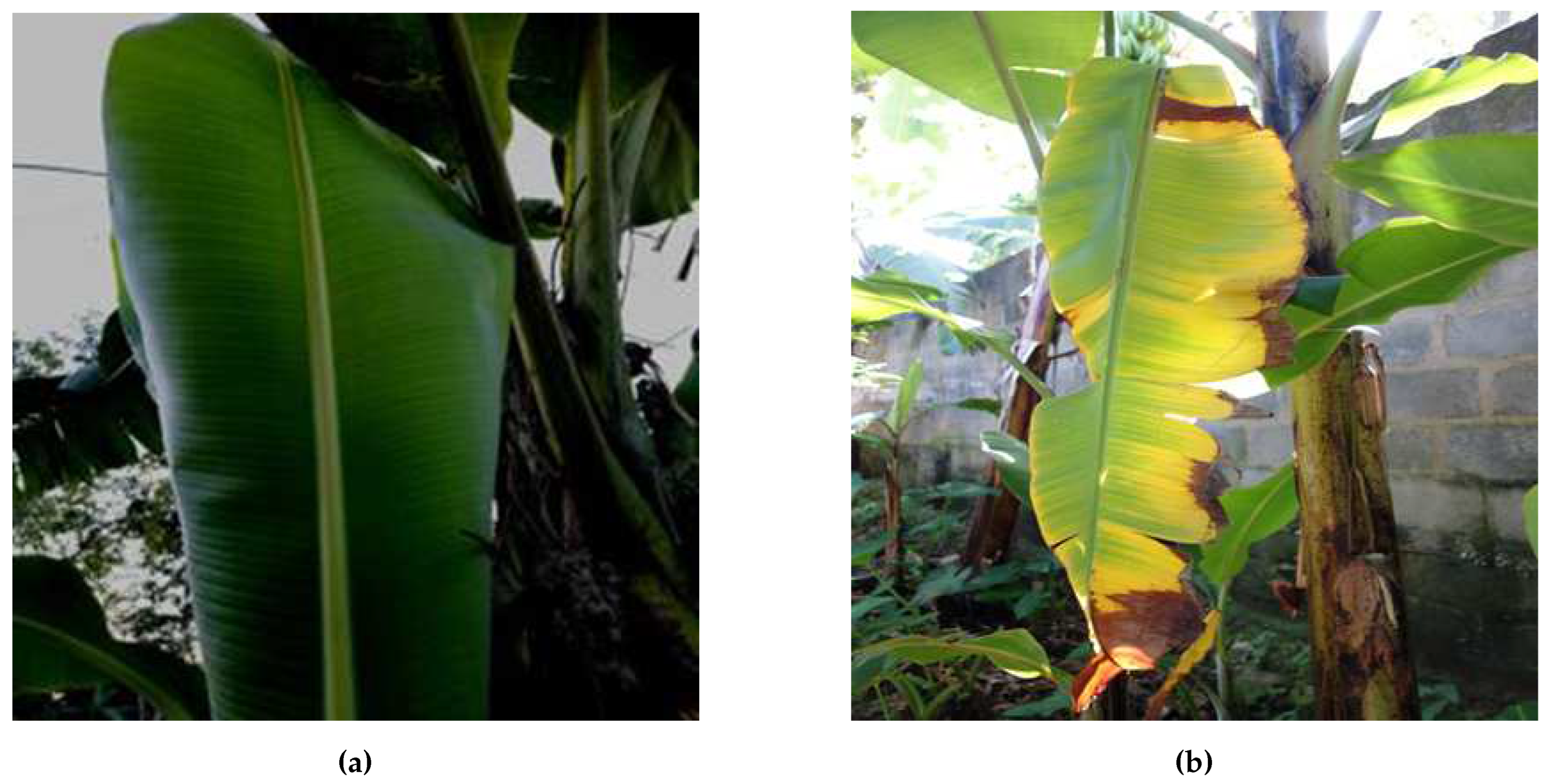
Figure 1. A comparison between healthy and diseased banana leaves: (a) An image of a healthy banana leaf and (b) An image of a Panama-diseased banana leaf.

Figure 1. A comparison between healthy and diseased banana leaves: (a) An image of a healthy banana leaf and (b) An image of a Panama-diseased banana leaf.

2.2. Data Pre-processing and Augmentation

To enhance the size of the initial dataset of banana leaf images and mitigate the risk of overfitting resulting from limited data, data augmentation techniques were employed. Random flipping, rotation, and noise addition were applied to expand the dataset, resulting in a collection of 300 images for each class. This augmented dataset served to provide the model with a richer and more diverse sample to train on, ensuring improved generalization capabilities beyond the original dataset.

The expanded dataset, now comprising a total of 600 labeled images, was partitioned into training and testing sets. This partitioning was carried out in an 80:20 ratio, with 0.80 of the images allocated to the training set, while the remaining 0.20 constituted the validation set. This division ensured that the model was trained on a substantial portion of the data while retaining a dedicated subset for performance evaluation and fine-tuning.

By establishing a clear distinction between the training and validation sets, the model’s performance could be effectively assessed and monitored during the training process. This separation allowed for a rigorous evaluation of the model’s ability to generalize its predictions to previously unseen data, ensuring that it could effectively detect and classify Fusarium wilt infection in banana crops beyond the images it had been trained on.

2.3. Transfer Learning

The goal of this study was to establish an efficient transfer learning-based CNN model for detecting Fusarium wilt infection in banana crops. Emphasis was placed on CNNs, which can be easily trained and deployed to facilitate wider use. To achieve this goal, we utilized the high-level neural network Application Programming Interface (API), Keras (Chollet et al., 2015), in conjunction with the machine learning framework TensorFlow (Abadi et al., 2015). We selected the popular CNN model ResNet-50 (He et al., 2016) due to its significant acclaim in the field of computer vision, particularly for its exceptional efficacy in image classification.

The ResNet-50 model we considered is available in Keras with pre-trained weights in the TensorFlow backend. This model was originally trained to recognize 1,000 different ImageNet (Russakovsky et al., 2015) object classes. In this paper, we modified the ImageNet-trained architecture of ResNet-50 to classify Fusarium wilt infection in banana crops. This modification involved replacing its last fully connected dense layer, which had 1,000 neurons, with a single-neuron fully connected layer.

2.4. Neural Network Architecture

The sequential structure of the CNN model ensures that each layer is stacked upon the previous one, enabling a systematic flow of information through the network. This sequential design facilitates the extraction of increasingly abstract features as the input image progresses through the layers.

2.5. Input Layer

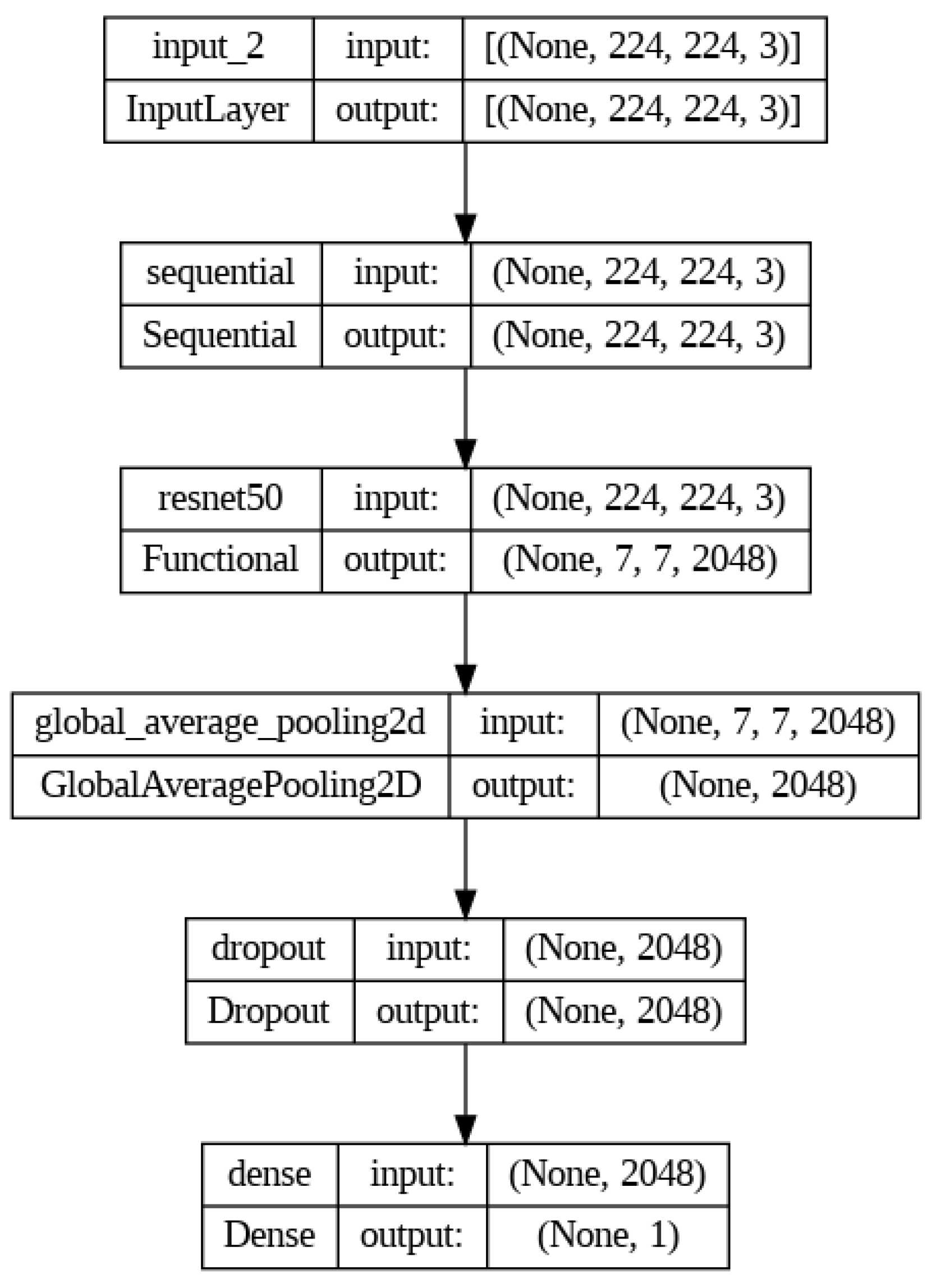
Figure 2 offers a comprehensive visualization of the CNN model’s architecture, illustrating the step-by-step transformation of the input image. The model begins with the input layer, which receives an image of size 224 x 224 pixels with three RGB values. The image is represented as a 3-dimensional matrix. Each cell in this matrix contains a pixel value, which, for grayscale images, represents the intensity of the pixel, and for RGB images, there are three matrices or channels corresponding to the Red, Green, and Blue components. This matrix is then fed to the convolutional layer.

2.6. Convolutional Layer

The ResNet-50 layer, represented as its own distinct layer in Figure 2, encompasses a series of components meticulously crafted to extract meaningful features. The initial convolutional layer performs convolutions on the input image, enabling the extraction of low-level features such as edges, corners, and textures. These low-level features play a crucial role in subsequent stages of the model.

Within the heart of the ResNet-50 model lies in its residual blocks, which are composed of multiple convolutional layers with increasing filters. These convolutional layers progressively capture complex and abstract features as the network delves deeper.

2.7. Max Pooling Layer

Following the initial convolutional layer, a max pooling layer is introduced to downsample the feature map. By reducing the spatial dimensions of the feature map, the max pooling layer extracts essential features while simultaneously enhancing computational efficiency. This reduction in size helps to highlight the most salient information while discarding irrelevant details.

2.8. Fully Connected Layer

The subsequent fully connected layer acts as a bridge between the convolutional layers and the final classification layer. It integrates the extracted features from the preceding layers and maps them to the appropriate dimensions for classification. This layer serves as a crucial component in aggregating and combining the representations learned throughout the network.

The last layer, the output layer, of the ResNet50 model is removed for the purposes of transfer learning. The only output layer used in the model will be at the end of the entire model as we have no need for probabilities of each prediction class to be output from the ResNet50 layer.

2.9. Global Average Pooling Layer

Once the information passes through the residual blocks, a global average pooling layer is applied. This layer reduces the spatial dimensions of the feature map by computing the average value of each feature map. By summarizing the information across the entire feature map, the global average pooling layer preserves the most relevant features while discarding spatial information. This process aids in focusing on the most descriptive aspects of the image.

2.10. Dropout Layer

After the global average pooling layer, a dropout layer is incorporated into the CNN model. The purpose of the dropout layer is to mitigate the risk of overfitting, a phenomenon in which the model becomes overly specialized to the training data and struggles to generalize well to unseen examples. By randomly dropping out a fraction of neurons during training, the dropout layer encourages the network to rely on a more diverse set of features and prevents excessive reliance on specific neurons. This regularization technique helps improve the model’s ability to generalize by reducing the likelihood of overfitting.

2.11. Output Layer

Finally, the CNN model concludes with a dense layer, which performs linear transformations on the input received from the previous layers. The dense layer’s role is to capture complex relationships and patterns in the extracted features. By applying appropriate weights and biases, the dense layer maps the transformed features to the desired output dimensions, ultimately aiding in the final classification task.

$$\begin{array}{c}\hfill \sigma \left(z\right)=\frac{1}{1+e^{-z}}.\end{array}$$

(1)

To generate classification probabilities for our specific problem, the dense layer utilizes the sigmoid activation function, specifically the logistic sigmoid function.

The sigmoid function, denoted in equation 1, transforms the output values of the layer into a range between 0 and 1. This property enables the model to interpret the resulting values as probabilities, representing the likelihood of a given input belonging to a particular class. By squashing the outputs within the desired range, the sigmoid activation provides normalized probabilities for each class. Each output neuron corresponds to a specific prediction class, in this case, Fusarium wilt or healthy.

3. Results

3.1. Training

Prior to the actual training of the model, the pre-trained layers of the ResNet-50 model were frozen. By freezing the pretrained layers, they can be used as fixed feature extractors, allowing meaningful features to be extracted from the new dataset without modifying the learned representations. These layers will later be unfrozen to fine-tune the model after training.

The CNN model was trained on Google Colab using the aforementioned Panama disease dataset. The training was accelerated using the cloud-based Graphics Processing Unit (GPU). The CNN model was trained with a range of epochs, spanning from 5 to 35, in order to determine the optimal training duration. It was found that a training time of approximately 17 epochs yielded the best results. This careful exploration was necessary to strike a balance between underfitting and overfitting.

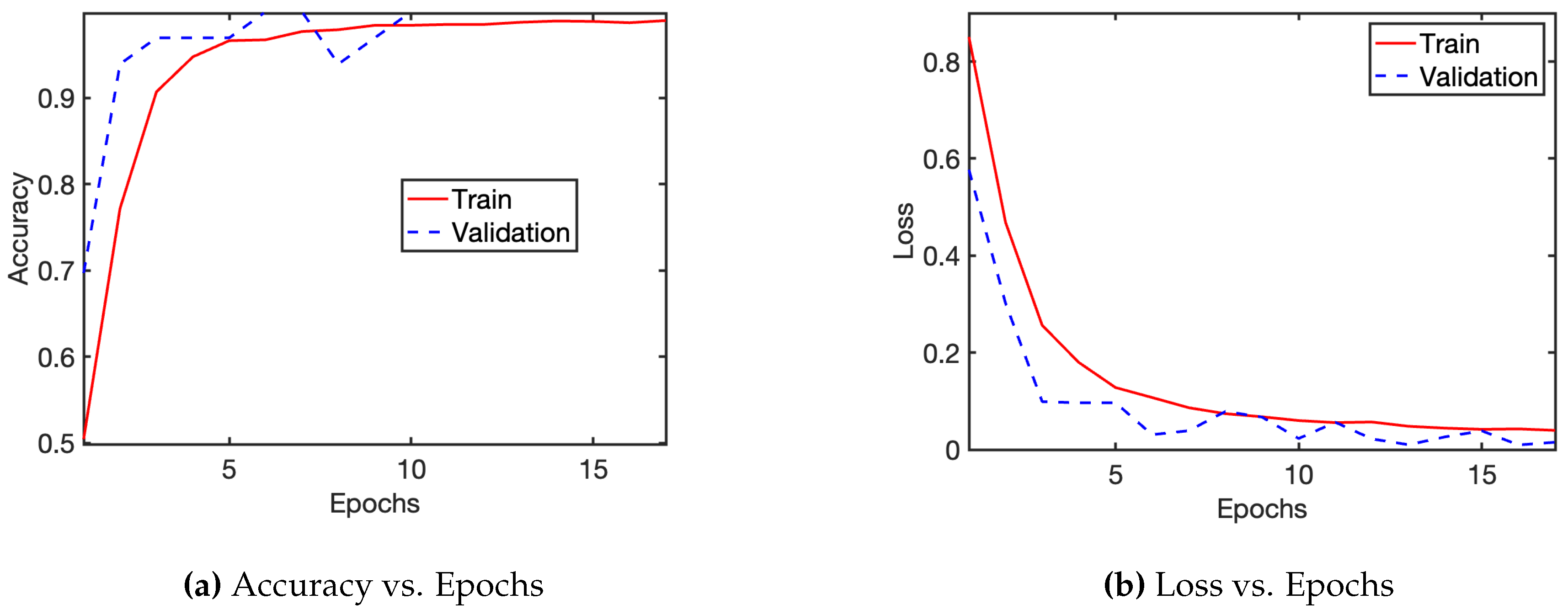
After the training, the CNN model achieved an accuracy of approximately 0.99, meaning it correctly classified 0.99 of the input samples. Additionally, the model achieved a relatively low loss value of around 0.1, indicating a small discrepancy between the predicted and actual values (see Figure 5 and Figure 6).

It is worth noting that during the training phase, both the accuracy and loss of the model exhibited an similar trend. Around the 8-epoch mark, the model experienced both its highest accuracy and its lowest loss (see Figure 5 and Figure 6). This suggests that the model rapidly grasped the essential patterns within the data, leading to a notable improvement in its predictive performance.

Figure 3. Visualization of the learning process where the training and the validation accuracy for our CNN model improve after successive epochs.

Figure 3. Visualization of the learning process where the training and the validation accuracy for our CNN model improve after successive epochs.

3.2. Fine Tuning

During the process of fine-tuning, the ResNet-50 layers of the CNN model were initially unfrozen for the entire model to be tuned. The learning rate of the model was also adjusted to 10^-5. This is done to ensure that the weights of the model are not drastically altered during this process. By fine-tuning, we are essentially adapting the knowledge of the base model to this identification task.

Figure 4. These outputs are the values of accuracy and loss of the training and validation sets during fine-tuning.

Figure 4. These outputs are the values of accuracy and loss of the training and validation sets during fine-tuning.

3.3. Model Evaluation

In order to determine the ability of the CNN model in identifying fusarium wilt infections, it was tested on a dataset consisting of 500 images.1 The images, previously unseen by the model, were taken from a google search. Using the OpenCV-Python3 library, the data augmentation techniques of rotation, noise addition, and resizing were used to expand the 200 healthy and diseased images to 500 images.

The metrics used to determine the overall performance of the model were: accuracy, precision, recall, and F-1 score. These measures are calculated using equations (1), (2), (3), and (4), respectively. Accuracy is a straightforward metric that measures the overall correctness of the model’s predictions. Precision is a metric that focuses on the positive predictions made by the model. It is defined as the ratio of true positive predictions (correctly predicted positive samples) to the total number of positive predictions (both true positives and false positives). Recall, also known as sensitivity or true positive rate, measures the ability of the model to correctly identify positive samples. It is defined as the ratio of true positive predictions to the total number of actual positive samples (true positives and false negatives). The F-1 score is the harmonic mean of precision and recall. It provides a balanced measure that considers both precision and recall simultaneously. Additionally, a confusion matrix was visualized through the OpenCV library packages to see the exact number of true and false positive and negative identification classes. It should be noted that the accuracy of random guessing identification for fusarium wilt will yield an accuracy of 0.50. It should also be noted that there is no method to truly quantify the accuracy of a farmer in identifying fusarium wilt as this depends on many variables including experience, age, genetics and more.

$$\begin{array}{cc}\hfill \mathrm{Accuracy}& =\frac{\mathrm{TP}+\mathrm{TN}}{\mathrm{TP}+\mathrm{TN}+\mathrm{FP}+\mathrm{FN}}.\hfill \end{array}$$

(2)

$$\begin{array}{cc}\hfill \mathrm{Precision}& =\frac{\mathrm{TP}}{\mathrm{TP}+\mathrm{FP}}.\hfill \end{array}$$

(3)

$$\begin{array}{cc}\hfill \mathrm{Recall}& =\frac{\mathrm{TP}}{\mathrm{TP}+\mathrm{FN}}.\hfill \end{array}$$

(4)

$$\begin{array}{cc}\hfill \mathrm{F}1\mathrm{Score}& =\frac{2\times \mathrm{Precision}\times \mathrm{Recall}}{\mathrm{Precision}+\mathrm{Recall}}.\hfill \end{array}$$

(5)

The CNN model was able to correctly identify 492 out of the 500 total test images to the correct classification class (see Figure 5). The 8 errors consisted of 5 false positive and 3 false negative identifications. The greater number of false positives in this case is considered a more desirable outcome because the farmer can verify that the banana crop is not truly infected before any potential removal of the entire plant. If the number of false negatives were to be higher, that would pose a larger issue of missing infections, and thus, allowing a greater spread of fusarium wilt.

Figure 5. The confusion matrix represents the predictions made by the CNN model (500 total predictions).

Figure 5. The confusion matrix represents the predictions made by the CNN model (500 total predictions).

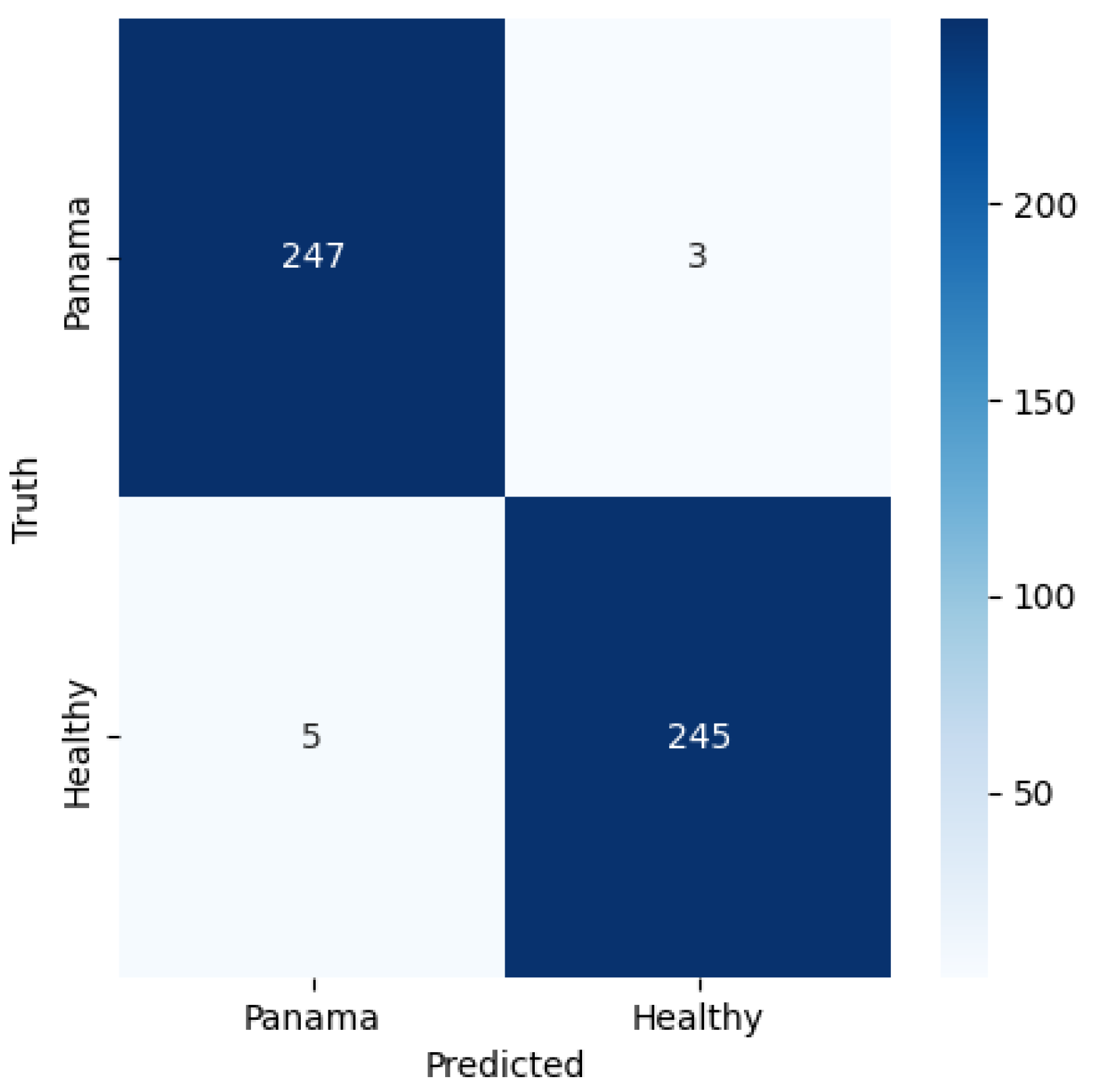
Figure 6. The classification report shown here depicts the precision, recall, F-1 score, accuracy, and the macro and weighted averages of these values.

Figure 6. The classification report shown here depicts the precision, recall, F-1 score, accuracy, and the macro and weighted averages of these values.

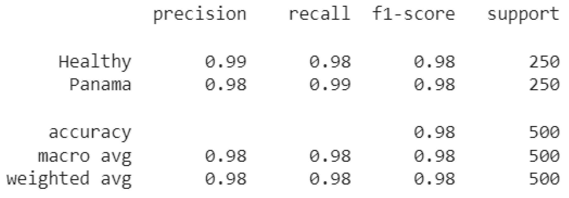
The CNN model was able to perform with an accuracy of 0.99 on the healthy images and 0.98 on the fusarium wilt diseased images. These measures combined with the 0.98 F1 score show the model was able to generalize its prior training to new data. As a comparison for metrics, (Sangeetha et al., 2023) trained a deep learning model to identify fusarium wilt and was only able to achieve 0.9156 accuracy, 0.9161 of precision, 0.8856 of recall, and 0.8156 of score. Their model was also able to substantially outperform existing models with an accuracy nearly 0.20 higher than the 2nd best model compared in their study. The model in this paper was able to outperform all the metrics of their model, however, this may be due to the original size of the evaluation set being substantially less than the set in their paper. In future real-world testing, this CNN model may yield slightly lower metrics; however, it is still expected that the model will outperform most existing models based on its stellar performance on this dataset.

This convolutional neural network approach to disease detection can be used in a wide range of applications in the future. Current industries where this technology is used include medicine, agriculture, transportation, astronomy, and many others. The model developed in this paper can be trained to identify many other banana diseases such as black sigatoka, banana mosaic virus, and banana bunchy top virus. The limitation of this study was the inability to perform real-world evaluation of the model due to the low availability of banana farms in the proximity of the southern United States. The next step for this system would be to test and implement it on a real-world banana plantation.

4. Discussion

The CNN model proposed in this paper was able to identify fusarium wilt infected banana leaves with both accuracy and precision. The accuracy of the model was able to reach around 0.98, significantly outperforming other similar models. This was done with a relatively small amount of model training time (17 epochs executed in under one hour), made substantially lesser by the use of the Google Colab GPU. Additionally, a relatively small dataset of 200 initial images, expanded into 600 total images by data augmentation, was successfully used in the training of this model. Despite the small dataset, the model was able to quickly learn the trends and differences between the healthy and diseased banana leaf images and achieve an accuracy of 0.99 after initial training. The accuracy of this model compared to current options shows the immediate potential for the model to be adapted into identification systems such as Unmanned Aerial Vehicles (UAVs) or smartphone apps. These systems can be utilized by farmers across the world to rapidly identify infections of fusarium wilt on their plantations, leading to a decrease in banana crop yield lost to disease. In the future, computational speed increases will allow for models like this one to become far more accurate and able to generalize predictions to the real world. Furthermore, for a more robust model, real-world data collection performed on specific plantations can allow for the system to perform much better for those given plantations. Techniques such as federated learning can allow for farmers and researchers to customize identification models to their specific crops. The innovative technologies of Generative adversarial networks (GANs) can also be leveraged to create larger amount of high-quality synthetic training data that is able to mimic real-world data for applications such as the one of this paper.

References

- Abadi, M.; Agarwal, A.; Barham, P., et al. TensorFlow: Large-Scale Machine Learning on Heterogeneous Systems. Available online: https://www.tensorflow.org/ (accessed on Day Month Year).
- Bharate, A.A.; Shirdhonkar, M.S. A review on plant disease detection using image processing. In Proceedings of the 2017 International Conference on Intelligent Sustainable Systems (ICISS); IEEE: 2017; pp. 103–109.
- Chaudhari, V.; Patil, M. Banana leaf disease detection using K-means clustering and Feature extraction techniques. In Proceedings of the 2020 International Conference on Advances in Computing, Communication & Materials (ICACCM); IEEE: 2020; pp. 126–130.
- Chollet, F., and others. Keras. Available online: https://github.com/fchollet/keras (accessed on Day Month Year).
- Geetharamani, G.; Pandian, A. Identification of plant leaf diseases using a nine-layer deep convolutional neural network. Computers & Electrical Engineering 2019, 76, 323–338.
- He, K., et al. Deep residual learning for image recognition. In Proceedings of the IEEE Conference on Computer Vision and Pattern Recognition; 2016; pp. 770–778.
- Heslop-Harrison, J.S.; Schwarzacher, T. Domestication, Genomics and the Future for Banana. Annals of Botany 2007, 100, 1073–1084. [CrossRef]
- Ibarra, N.C.; Rivera, M.P.; Manlises, C.O. Detection of Panama Disease on Banana Leaves Using the YOLOv4 Algorithm. In Proceedings of the 2023 15th International Conference on Computer and Automation Engineering (ICCAE); IEEE: 2023; pp. 209–214.
- Lin, B.; Shen, H. Fusarium oxysporum f. sp. cubense. In Biological Invasions and Its Management in China: Volume 2; 2017; pp. 225–236.
- Mahlein, A.K. Plant disease detection by imaging sensors–parallels and specific demands for precision agriculture and plant phenotyping. Plant disease 2016, 100, 241–251. [CrossRef]
- Medhi, E.; Deb, N. PSFD-Musa: A dataset of banana plant, stem, fruit, leaf, and disease. Data in brief 2022, 43, 108427. [CrossRef]
- Mukti, I.Z.; Biswas, D. Transfer learning-based plant diseases detection using ResNet50. In Proceedings of the 2019 4th International conference on electrical information and communication technology (EICT); IEEE: 2019; pp. 1–6.
- O’Shea, K.; Nash, R. An introduction to convolutional neural networks. arXiv preprint https://arxiv.org/abs/1511.08458.
- Ordonez, N.; Seidl, M.F.; Waalwijk, C.; Drenth, A.; Kilian, A.; Thomma, B.P.; Kema, G.H., et al. Worse comes to worst: bananas and Panama disease—when plant and pathogen clones meet. PLoS pathogens 2015, 11, e1005197. [CrossRef]
- Pandian, J.A.; Kumar, V.D.; Geman, O.; Hnatiuc, M.; Arif, M.; Kanchanadevi, K. Plant disease detection using deep convolutional neural network. Applied Sciences 2022, 12, 468. [CrossRef]
- Redmon, J.; Farhadi, A. YOLOv3: An incremental improvement. arXiv preprint https://arxiv.org/abs/1804.02767.
- Ren, S.; He, K.; Girshick, R.; Sun, J. Faster r-cnn: Towards real-time object detection with region proposal networks. In Proceedings of the Neural Information Processing Systems (NeurIPS) Conference; 2015; pp. 91–99.
- Simonyan, K.; Zisserman, A. Very deep convolutional networks for large-scale image recognition. arXiv preprint https://arxiv.org/abs/1409.1556.
- Singh, S.; Mohanty, A.K.; Bhowmik, R.; Manogaran, G.; Gupta, D.; Kumar, R., et al. A collaborative multi-deep-learning model for human activity recognition system in IoT environment. Journal of Ambient Intelligence and Humanized Computing 2019, 10, 2877–2885.
- Szegedy, C.; Vanhoucke, V.; Ioffe, S.; Shlens, J.; Wojna, Z. Rethinking the inception architecture for computer vision. In Proceedings of the IEEE Conference on Computer Vision and Pattern Recognition (CVPR); 2016; pp. 2818–2826.
- Taherkhani, A.; Belatreche, A.; Li, Y.; Maguire, L.P. A review of learning in biologically plausible spiking neural networks. Neural Networks 2020, 122, 253–272. [CrossRef]
- Vu, H.T.; Upla, K.P.; Plataniotis, K.N. Capsule network for plant disease classification. PloS one 2020, 15, e0229772.
- Wang, C.; Zhang, H.; Wang, X.; Wu, X. A review on deep learning for plant disease prediction. Journal of King Saud University-Computer and Information Sciences 2022.
- Xie, S.; Girshick, R.; Dollár, P.; Tu, Z.; He, K. Aggregated residual transformations for deep neural networks. In Proceedings of the IEEE Conference on Computer Vision and Pattern Recognition (CVPR); 2017; pp. 1492–1500.
- Zoph, B.; Vasudevan, V.; Shlens, J.; Le, Q.V. Learning transferable architectures for scalable image recognition. In Proceedings of the IEEE Conference on Computer Vision and Pattern Recognition (CVPR); 2018; pp. 8697–8710.