Submitted:
23 September 2023
Posted:
26 September 2023
You are already at the latest version
Abstract
In order to meet the diversified rehabilitation needs of people, it is necessary to design a product for active rehabilitation of patients. Existing rehabilitation chairs use intelligent massage, which can cause problems such as large massage area, inability to local massage, large chair size, and inability to meet the continuous use of the damaged parts. In this paper, modular design method and multi-layer evaluation method are used to solve the problems related to rehabilitation chairs. The authors use the questionnaire survey method and the functional technology matrix method to determine the functional requirements of the rehabilitation chair, and then use the multilevel evaluation methods, including the AHP method, entropy weight method main and grey correlation analysis, to optimize the functional solutions of the rehabilitation chair, and finally obtain a chair for the rehabilitation of patients with upper and lower limb disorders. Problems such as generalisation of rehabilitation scope and non-durable use of components were solved, and the purpose of active exercise was achieved. This study verifies that the use of multilevel decision evaluation method can effectively improve the efficiency of programme decision-making, and provides theoretical and practical basis for the design of similar products.
Keywords:
product design
; rehabilitation chair
; AHP
; entropy weighting
; grey relational analysis
1. Introduction
Limb movement dysfunction is one of the most common rehabilitation problems in patients with stroke, hemiplegia, ageing and chronic diseases [1]. It is estimated that by 2047, older people will outnumber children globally [2]. Research and improvement of rehabilitation products can improve the quality of rehabilitation for people with physical disabilities. Currently, most of the product designs related to the rehabilitation of physical disabilities are exoskeleton devices or positioning and massage rehabilitation robots [3-4]. The design of rehabilitation robots began in the 1980s, and MIT-Manus was one of the first organisations to develop rehabilitation robots, which are important for achieving functional compensation and reconstruction for patients with disabilities [5-9]. The process of limb rehabilitation is a long and slow process, and existing rehabilitation products mainly focus on localised limb rehabilitation and cannot provide full-cycle and multi-stage rehabilitation use. Due to the complexity of the upper and lower limb interaction structure, products that realise simultaneous rehabilitation of the upper and lower limbs will inevitably increase the cost, which necessitates the use of the concepts of sustainable development and circular economy to manufacture rehabilitation products [10]. Dividing a complex product system into different types of components and then considering their functions, manufacturing and interworking processes has the advantage of reducing the complexity of product development and improving resource utilisation. In conclusion, this study presents a rehabilitation chair design that aims to promote products for the active rehabilitation of patients with upper and lower limb dysfunction by promoting self-rehabilitation of physically disabled people.
The remaining sections of this paper are structured as follows. In Section 2, the authors briefly review the literature on the methodology of the study, the shortcomings of previous studies, and areas for improvement and innovation in this research area. In Section 3, the authors introduce the research framework for the design of the rehabilitation chair and systematically discuss the design process of each functional structure of the rehabilitation chair. Section 4 demonstrates the specific structure and use of the final preferred solution for the rehabilitation chair and discusses the methodology and experience used for the modular rehabilitation chair. Section 5 is the concluding section which summarises the innovations in the design of the modular rehabilitation chair and provides some ideas for future research directions to extend the scope of this study.
2. Materials and Methods
2.1. Design Process
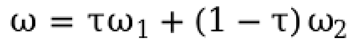
Using the questionnaire research method, the functional analysis method and the multi-level evaluation method, the design functions were gradually specified. Through questionnaire interviews with relevant personnel from three elderly care institutions in Changsha City, we collected the current demand for rehabilitation chairs for patients with upper and lower limb impairments from 300 questionnaires, which were screened to establish a functional technology matrix. Then the different combination forms of each functional technology pathway were analysed, and feasible design solutions were determined. Finally, the multilevel fuzzy comprehensive evaluation methods, i.e., AHP method, entropy weight method and grey correlation analysis method, were combined to determine the final design scheme of the rehabilitation chair [11-17].The specific steps are shown in Figure 1.
2.2. Functional Requirement Analysis of Rehabilitation Chairs
The authors observed the physically disabled groups in three nursing homes in Changsha, Hunan Province, namely Taikang Home Xiangyuan, Poly Changsha Tianxinyuehui, and Changsha Puzhen Nursing Home, and the main observations are as follows: 1. How long physically disabled people use it every day; 2. Whether they need rehabilitation chairs in their daily rehabilitation training; 3. What rehabilitation functions are needed to meet the stage-by-stage rehabilitation needs; 4. How the functional modules are laid out in order to effectively Reduce the cost. Through the collation of the functional requirements of the rehabilitation chair as shown in Figure 2: the main functions of upper limb rehabilitation are: back massage,stretching, chest expansion, arm raising,grasping; the main functions of lower limb rehabilitation are: flexion, stretching, leg lifting, foot sports, leg tapping.
Figure 2.
Rehabilitation Chair Functional Requirements.
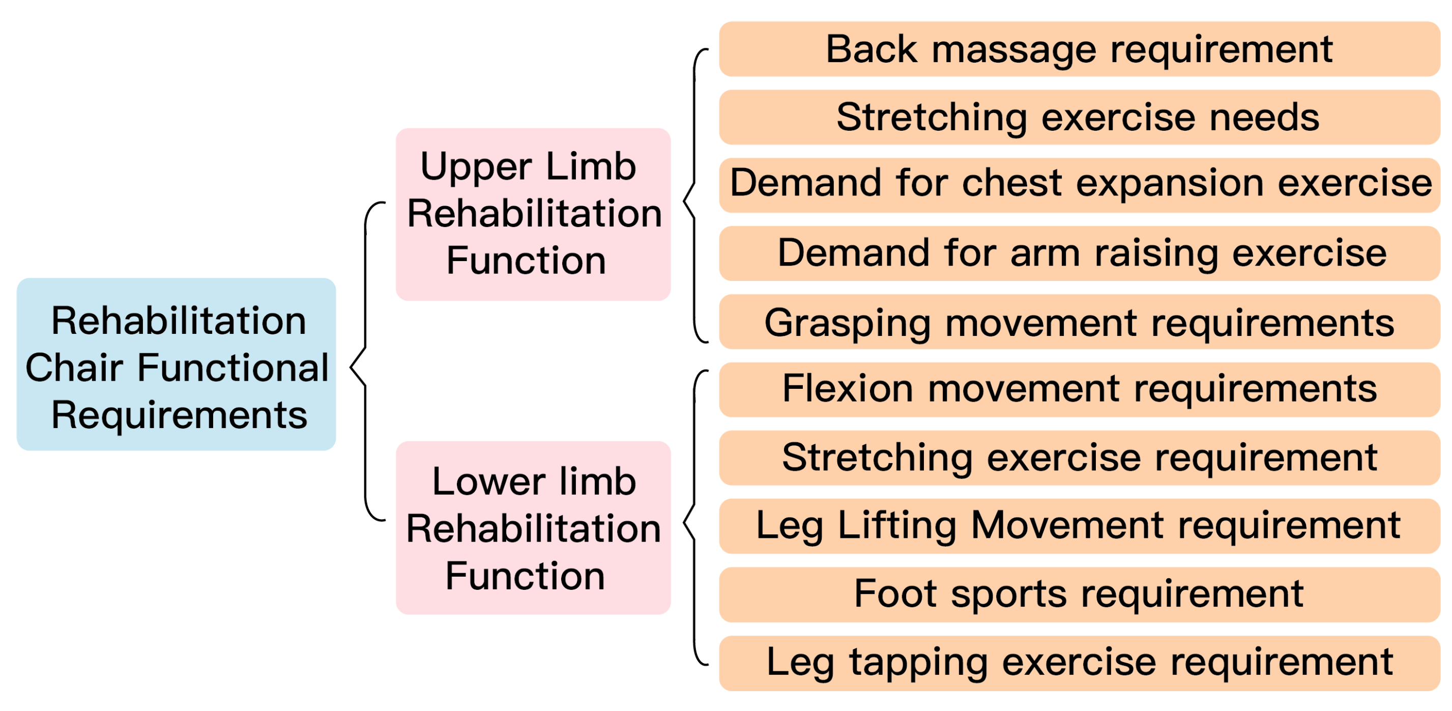
Figure 1.
This is a figure. Schemes follow the same formatting.
2.3. Establish a Modular Rehabilitation Chair Functional Technology Matrix
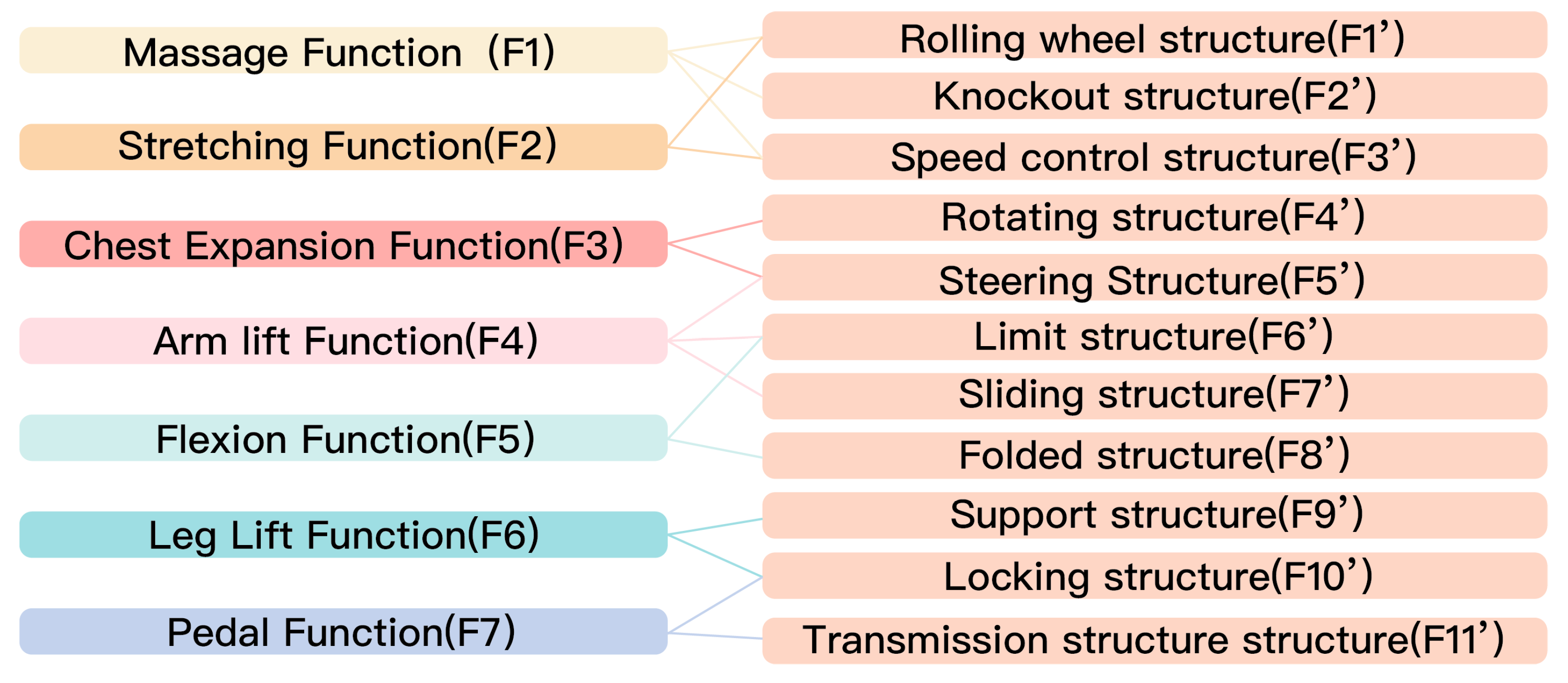
The total function of the rehabilitation chair is decomposed until it is broken down to the functional elements composed of structures or parts, as shown in Figure 3. The decomposed functional elements are established into functional technical matrix diagrams, and the technical pathways of each functional element are comprehensively analyzed to find the functional module design solution with high practical value, sustainable use, technical and economic superiority and aesthetics. The specific steps are as follows:
Step 1:Total functions are divided into functional elements
Organize each functional element according to the realization relationship between functions. Distinguish between essential and non-essential functions according to the degree of importance of the functions, and distinguish between the subordinate and superior relationships of the functions according to the relationship between ends and means,as shown in Figure 3.
Step 2:Functional Technology Matrix Analysis
The functional matrix is a sequence of rehabilitation functions around which different forms of combinations of supporting technologies to achieve each function are analyzed qualitatively or quantitatively to find reliable solutions, as shown in Table 1.
Step 3:Functional sequence importance coefficient rating
Functional importance coefficient is also known as functional coefficient or functional index. Rehabilitation chair functional importance coefficient rating is based on the different roles of each functional element in the overall system, through the mandatory scoring method (0-1 or 0-4 scoring method), multi-proportional scoring method, logical scoring method, ring scoring method, etc. This paper uses the 0-4 scoring method, that is, 10 professionals are invited to compare between two functional elements, specifically: the very important functional element scores 4 points, another very important function element scores 1; the more important function element scores 3, the other less important function element scores 1; when equally important or basically equally important, the two function elements score 2 each, very unimportant score 1, and no score for their own comparison. As shown in Table 2, a massage function of 0.174, a stretching function of 0.130, a chest expansion function of 0.081, an arm lift function of 0.174, a flexion function of 0.093, a leg tapping function of 0.093, and a foot pedal function of 0.174 were obtained.
Step 4: Construct the Functional Technical Matrix
Based on the results of the rating of functional importance factors, the functional technology matrix was constructed. In order to expand the scope of the technology pathway and improve the creativity and effectiveness of the final solution, the latest scientific research results and manufacturing technologies were adopted as the technology pathway for the rehabilitation chair. Table 3 shows the functional technology path of the rehabilitation chair, in which the massage function mainly utilises structures such as rollers, worm gear structures and struts, the extension function mainly utilises structures such as rollers, socketed telescopic sliders and telescopic sliders, the chest expansion function mainly utilises structures such as screws, chucks, mandrels and telescopic rods, the arm lift function mainly utilises structures such as supports, rotating sections and rotating telescopic sections, and the flexion function mainly Flexion function mainly utilises folding rod ends, locking rings and fixing pins, Leg knocking function mainly utilises wooden knockers, support wheels and hinged rods, Pedal function mainly utilises turntables, connecting plates and foot pedals.
Step 5:Comprehensive analysis of the technical approach
Technical pathway comprehensive analysis refers to a comprehensive consideration of the technology, cost, utility, aesthetics and other indicators used in the design of the rehabilitation chair. The scoring items are developed according to the requirements, and the scoring method refers to the 0-4 scoring method. The scoring items of the functional elements of the rehabilitation chair include technicality, environmental protection, and applicability, and each functional element is compared one-to-one to obtain Table 4, Table 5 and Table 6.
Step 6:Technology compatibility analysis
Technology compatibility analysis is an important method to determine whether the combination of technology paths of each functional element is compatible with each other and the feasibility of the combination scheme.The N*N order matrix is constructed using the adjacency matrix method to perform the technical pathway compatibility analysis, as shown in Table 7. If the combination condition is feasible, it is counted as 1, and if the combination condition is not feasible, it is counted as 0. The technical pathway ratings of T1, T2, T3...etc. are performed sequentially, and finally a number of combination schemes Q are obtained.
Q={q1,q2,qn,...,qm,}
Here, qn is the nth feasible solution, m is the number of feasible solutions
Step 7: Determine a feasible functional solution for the rehabilitation chair
As shown in Table 7, the pathways with higher technical excellence index coefficient scores in Table 4 were subjected to technical compatibility matrix analysis, with compatibility as 1 and incompatibility as 0. The feasible options for the rehabilitation chair function were obtained as follows:
(1) massage function: roller, worm gear worm gear, strut
(2) stretching function: sleeve type expansion slider,telescopic slider
(3) chest expansion function: screw,mandrel
(4) arm lift function: support piece, rotating section
(5) flexion function: folded movable rod end, retaining pin
(6) leg tapping function: wooden knockout head, hinge rod
(7) pedal function: turntable, foot pedal
Step 8: Design the functional of the rehabilitation chair
Referring to Professor Salter’s concept of continuous passive movement (CPM), the back massage function scheme, the lower limb exercise function scheme, and the leg rehabilitation massage function scheme of the rehabilitation chair are designed for the three phases of rehabilitation training (passive movement in the early stage of rehabilitation, assisted active movement in the middle stage of rehabilitation, and impedance movement in the late stage of rehabilitation), as shown in Figure 4-6.
In the backrest massage function there are three schemes, as shown in Figure 4. In the first scheme, the sphere 11 is used as the structure to support and connect the double backrests, and the right backrest and the left backrest have the same structure. The left backrest drives the worm gear 8 to rotate through the armrest 3, and the worm gear 8 drives the worm gear 5, worm gear 7 and worm gear 9 to rotate in turn, at which time the worm gear 5 and worm gear 9 drive the roller 2 and roller 4 to massage the back. When the armrest 3 is in the default state, the double-layer backrest structure is opened outward with the worm gear 8 as the rotation centre, and the sphere 11 controls the stability of the double-layer backrest, which can meet the user’s chest expansion movement. In the second option, the backrest is designed as four pieces, which can improve the massage range and accuracy. Worm wheel 23 rotates with the armrest, and at the same time drives worm wheel 17 and worm wheel 24 for massage. When the armrests are opened outwards, the support connectors 22 control the left and right sides of the backrest in a breast expansion movement. In the third option, the left and right sides of the backrest are connected by 4 telescopic rods 32. In the massage function, the 4 hexagonal body blocks behind the left side of the backrest drive the connector 31, connector 33, connector 35 and connector 36 to rotate respectively, and the massage rollers rotate and massage accordingly.
In the lower limb movement function module, as shown in Figure 5, there are three schemes. In the first scheme, the turn Table 2 rotates around the rod member 4, and the foot pedal 5 rotates and unfolds around the mandrel 6 to reach the foot pedal state. In the second embodiment, the telescopic rotary member 7 connects the ball connector 8 and the rod member 9 to drive the roller 12 and the roller 13 upwardly to achieve the function of extending and lifting the leg. In the default state, the foot pedal 14 is used to drive the roller 12 and the roller 13 to complete the foot rehabilitation function. In the third embodiment, the connecting member 18 rotates around the shaft 17 to achieve the leg extension and lifting function. The foot pedal 16 is used to drive the rollers 15 to fulfil the foot rehabilitation function.
There are three scenarios for the outer leg massage, as shown in Figure 6. In the first scheme, the connecting rod 5 and the connecting rod 4 rotate around the roller 6 and the roller 4, which can control the massage height and the massage angle. The percussion head 3 is provided on a mandrel 2 inside the armrest, which rotates around the linkage 1. In a second embodiment, the percussion structure is designed on both sides of the seat surface, and the percussion structure slides forward with the mandrel 9. The hand control panel 12 rotates with the mandrel 8 and drives the wooden knocking head 7 to fulfil the leg knocking function. In the third embodiment, the wooden knocking head 13 is embedded in the mandrel 14 within the armrest, and the armrest rotates to complete the knocking function.
2.4. AHP-Entropy Theory Based Grey Correlation Method Scheme Evaluation Process
Using the gray correlation method to get the correlation degree of each functional scheme, then using the AHP-Entropy weight method to calculate the comprehensive weight, and finally calculate the gray weighting weight of each scheme to get the optimal scheme, the process is shown in Figure 1.
Establish a modular decision evaluation system for the rehabilitation chair program, as shown in Figure 4,the evaluated program is C(C=1,2,3, n), the set of assessment level indicators is E’=(E’1),The set of secondary indicators is E’=E’1m,E’2m,E’3m,...,E’nm)}, then the evaluation steps are as follows:
Step 1: Determine the reference data column
Determine the optimal value of each index as the reference data column, and set the reference data column as E’0=E’01,E’02,E’03,...,E’0m).
Step 2:Data normalization
To improve the validity of the data, the different indicators are normalized. The comparison matrix E=(Enm=(E’Jk)nm=(J=[1,m]; k=[1,n]) was obtained.
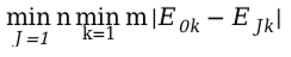
Step 3:Determine the extreme values
Two levels of absolute difference:
Maximum difference:
Minimum difference:
Step 4:Calculation of correlatio coefficients
The correlation coefficient represents the correlation between the comparison series and the reference series at a certain value. The correlation coefficient is calculated according to equation (5), in which the smaller ρ is the stronger the difference between the correlation coefficients[18].

Here, ρ is the resolution factor and take the value of 0.5
Step 5:Calculate the correlation
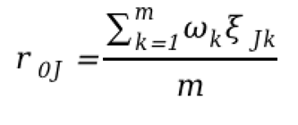
Calculate the average value of the correlation coefficient between each index and the reference series at a certain value[19].
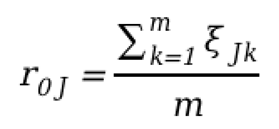
Here, ξJk is the correlation between the comparison series and the reference series; m is the number of evaluation indicator.
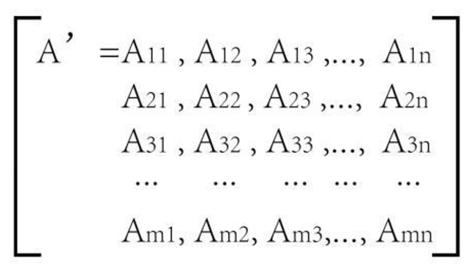
Step 6: Establishing judgment atrix
The 9-point scale method was used to score each assessment index for a two-by-two comparison, and the scoring criteria were shown in Table 8 to establish a judgment matrix A’={A1m,A2m,A3m,...,Anm}.
Step 7:AHP method to calculate subjective weights
The AHP method can decompose complex problems into base units and group them according to their inter-dominant relationships to form an ordered progressive hierarchy, and then determine the relative importance of each base unit by two-by-two comparison[15].
(1) Establishing judgment matrix
The 9-point scale method was used to score each evaluation index for two comparisons and establish the judgment matrix A’[20].
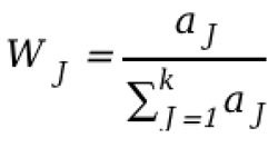
(2) Calculation of relative weights
The scalar product of each row is calculated according to Equations 8-9, and then its geometric mean is determined.
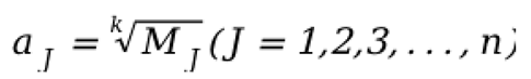
(3)Calculate the maximum characteristic value of each evaluation index[42]
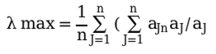
Here, aJn is the nth component of the vector aJ and n is the number of steps
(4)Consistency test
Calculating the consistency ratio:
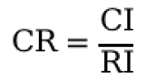
CI=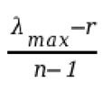
Here,RI is the average random consistency index; CR is the consistency ratio. CR≤0.1 indicates that the consistency test is passed, and vice versa, it is failed.
Step 8:Entropy weighting method to calculate objective weights
(1) Convert the scoring matrix into a normalized matrix
The assessment indicators in the matrix are normalized according to Equation 13:
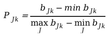
Here, PJk is the normalized decision matrix, bJk is the original matrix value, J=1,2,...,m, k=1,2,... ,m, k=1,2,... ,n.
(2) Determine the entropy of each evaluation index
Calculate the entropy value of the kth indicator according to Equation 14:
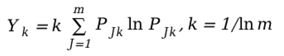
Here, Yk is the information entropy of each indicator, and the smaller Yk represents the higher dispersion of the data under k indicators and the greater amount of information provided.
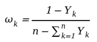
(3) After defining the entropy of the k indicators, the entropy weights can be obtained as follows:
Step 9:Gray weighted composit weight calculation
Calculate the average of the correlation coefficients between each indicator and the reference series at a certain value according to Equation 16:
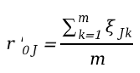
Here, ξJk is the correlation between the comparison series and the reference series; m is the number of evaluation indicators.
The gray weighted correlation is calculated and ranked according to Equation 17, and the top-ranked scheme is the preferred scheme. The indicators with high weight and low score in the design scheme need to be optimized to a high degree[16].
Here, ωk is the weight value of the kth assessment index; ξJk is the correlation between the kth assessment index of the Jth product and the reference series .
2.5. Gray Evaluation Results Based on AHP-Entropy Weight Theory
The optimal solution of each assessment index is set as the reference sequence, i.e., (E0) = (5, 5, 5, 5, 5, 5, 5, 5, 5, 5, 5, 5, 5, 5, 5, 5, 5, 5, 5, 5, 5, 5, 5, 5, 5, 5, 5, 5, 5, 5, 5, 5, 5, 5, 5, 5, 5, 5), and the value taken in the correlation coefficient is determined as 0.5. The smaller the ρ in the formula for calculating the correlation coefficient, the greater the discriminative power[17]. The results of the correlation coefficient calculation are shown in Table 9.

Table 9.
Calculation results of the correlation coefficient of each functional module scheme.
| Backrest 1 | Backrest 2 | Backrest 3 | Lower Limb1 | Lower Limb2 | Lower Limb3 | Handrail 1 | Handrail 2 | Handrail 3 |
|---|---|---|---|---|---|---|---|---|
| 0.691 | 0.724 | 0.802 | 0.639 | 0.794 | 0.613 | 0.692 | 0.732 | 0.731 |
| 0.765 | 0.697 | 0.647 | 0.753 | 0.667 | 0.712 | 0.669 | 0.809 | 0.639 |
| 0.848 | 0.860 | 0.771 | 0.743 | 0.710 | 0.712 | 0.673 | 0.772 | 0.673 |
| 0.715 | 0.695 | 0.545 | 0.643 | 0.636 | 0.686 | 0.727 | 0.789 | 0.749 |
| 0.766 | 0.762 | 0.714 | 0.736 | 0.653 | 0.720 | 0.658 | 0.783 | 0.773 |
| 0.742 | 0.744 | 0.744 | 0.793 | 0.764 | 0.679 | 0.641 | 0.815 | 0.745 |
| 0.639 | 0.678 | 0.590 | 0.590 | 0.686 | 0.717 | 0.769 | 0.745 | 0.746 |
| 0.666 | 0.742 | 0.707 | 0.676 | 0.710 | 0.725 | 0.666 | 0.687 | 0.794 |
| 0.756 | 0.827 | 0.650 | 0.607 | 0.697 | 0.697 | 0.861 | 0.784 | 0.859 |
| 0.675 | 0.713 | 0.734 | 0.659 | 0.741 | 0.745 | 0.733 | 0.738 | 0.691 |
| 0.714 | 0.713 | 0.709 | 0.739 | 0.689 | 0.684 | 0.685 | 0.812 | 0.729 |
| 0.753 | 0.762 | 0.721 | 0.602 | 0.718 | 0.743 | 0.761 | 0.745 | 0.831 |
| 0.788 | 0.715 | 0.686 | 0.702 | 0.714 | 0.751 | 0.710 | 0.724 | 0.803 |
| 0.713 | 0.800 | 0.725 | 0.743 | 0.808 | 0.711 | 0.670 | 0.736 | 0.706 |
| 0.876 | 0.778 | 0.723 | 0.729 | 0.654 | 0.693 | 0.822 | 0.768 | 0.760 |
| 0.735 | 0.593 | 0.627 | 0.767 | 0.626 | 0.559 | 0.571 | 0.810 | 0.761 |
| 0.866 | 0.608 | 0.718 | 0.692 | 0.708 | 0.728 | 0.687 | 0.814 | 0.690 |
| 0.682 | 0.687 | 0.646 | 0.758 | 0.610 | 0.629 | 0.613 | 0.683 | 0.651 |
| 0.732 | 0.812 | 0.720 | 0.720 | 0.708 | 0.729 | 0.693 | 0.750 | 0.779 |
| 0.663 | 0.846 | 0.652 | 0.718 | 0.703 | 0.661 | 0.710 | 0.840 | 0.679 |
| 0.591 | 0.748 | 0.720 | 0.603 | 0.698 | 0.646 | 0.692 | 0.676 | 0.792 |
| 0.774 | 0.708 | 0.762 | 0.624 | 0.728 | 0.642 | 0.615 | 0.850 | 0.720 |
| 0.692 | 0.729 | 0.680 | 0.588 | 0.803 | 0.667 | 0.717 | 0.680 | 0.801 |
| 0.631 | 0.833 | 0.762 | 0.582 | 0.756 | 0.701 | 0.759 | 0.797 | 0.893 |
Table 10.
Relevance results of each functional module solution and its ranking.
| Programs | Backrest 1 | Backrest 2 | Backrest 3 | Lower Limb1 | Lower Limb2 | Lower Limb3 | Handrail 1 | Handrail 2 | Handrail 3 |
|---|---|---|---|---|---|---|---|---|---|
| Relevance | 0.728 | 0.741 | 0.698 | 0.684 | 0.708 | 0.690 | 0.700 | 0.764 | 0.750 |
| Ranking | 2 | 1 | 3 | 3 | 1 | 2 | 3 | 1 | 2 |
Table 11.
Table of subjective weights calculated by AHP.
| Primary Indicators | Secondary indicators | Contrast matrix | Eigenvector | Subjective weights | λmax | CR | |||
|---|---|---|---|---|---|---|---|---|---|
| E1 | E11 | 1 | 3 | 1/3 | 3 | 1.022 | 0.25547 | 4.162 | 0.061 |
| E12 | 1/3 | 1 | 1/3 | 3 | 0.606 | 0.15157 | |||
| E13 | 3 | 3 | 1 | 7 | 2.105 | 0.52614 | |||
| E14 | 1/3 | 1/3 | 1/7 | 1 | 0.267 | 0.06681 | |||
| E2 | E21 | 1 | 3 | 1/3 | 3 | 1.102 | 0.27548 | 4.249 | 0.094 |
| E22 | 1/3 | 1 | 1/2 | 3 | 0.725 | 0.18131 | |||
| E23 | 3 | 2 | 1 | 5 | 1.867 | 0.46678 | |||
| E24 | 1/3 | 1/3 | 1/5 | 1 | 0.306 | 0.07644 | |||
| E3 | E31 | 1 | 1/3 | 1/2 | 1/3 | 0.437 | 0.10926 | 4.261 | 0.098 |
| E32 | 3 | 1 | 1/3 | 1/2 | 0.792 | 0.19812 | |||
| E33 | 2 | 3 | 1 | 1/2 | 1.171 | 0.29277 | |||
| E34 | 3 | 2 | 2 | 1 | 1.599 | 0.39986 | |||
| E4 | E41 | 1 | 1/3 | 1/2 | 3 | 0.728 | 0.01820 | 4.215 | 0.081 |
| E42 | 3 | 1 | 3 | 3 | 1.894 | 0.47359 | |||
| E43 | 2 | 1/3 | 1 | 3 | 0.989 | 0.24734 | |||
| E44 | 1/3 | 1/3 | 1/3 | 1 | 0.388 | 0.09707 | |||
| E5 | E51 | 1 | 1/2 | 1/3 | 1/2 | 0.422 | 0.10545 | 4.215 | 0.081 |
| E52 | 2 | 1 | 1/3 | 1/2 | 0.681 | 0.17032 | |||
| E53 | 3 | 3 | 1 | 1/2 | 1.282 | 0.32047 | |||
| E54 | 3 | 2 | 2 | 1 | 1.615 | 0.40376 | |||
| E6 | E61 | 1 | 1/2 | 3 | 3 | 1.237 | 0.30921 | 4.143 | 0.054 |
| E62 | 2 | 1 | 3 | 3 | 1.74 | 0.43508 | |||
| E63 | 1/3 | 1/3 | 1 | 1/2 | 0.423 | 0.10563 | |||
| E64 | 1/3 | 1/3 | 2 | 1 | 0.6 | 0.15008 | |||
| E7 | E11 | 1 | 3 | 1/3 | 3 | 1.022 | 0.25547 | 4.121 | 0.046 |
| E12 | 1/3 | 1 | 1/3 | 3 | 0.606 | 0.15157 | |||
| E13 | 3 | 3 | 1 | 7 | 2.105 | 0.52614 | |||
| E14 | 1/3 | 1/3 | 1/7 | 1 | 0.267 | 0.06681 | |||
Table 12.
Table of objective weights calculated by entropy weight theory.
| Evaluation metrics | Information entropy value e | Redundancy degree d | Objective weights |
|---|---|---|---|
| E11 | 0.362 | 0.638 | 0.38522 |
| E12 | 0.696 | 0.304 | 0.18326 |
| E13 | 0.599 | 0.401 | 0.24181 |
| E14 | 0.599 | 0.314 | 0.18971 |
| E21 | 0.361 | 0.639 | 0.40834 |
| E22 | 0.700 | 0.300 | 0.19187 |
| E23 | 0.625 | 0.375 | 0.23999 |
| E24 | 0.750 | 0.250 | 0.15980 |
| E31 | 0.761 | 0.239 | 0.17935 |
| E32 | 0.700 | 0.300 | 0.22524 |
| E33 | 0.580 | 0.420 | 0.31532 |
| E34 | 0.627 | 0.373 | 0.28010 |
| E41 | 0.700 | 0.300 | 0.14838 |
| E42 | 0.003 | 0.997 | 0.49302 |
| E43 | 0.482 | 0.518 | 0.25602 |
| E44 | 0.793 | 0.207 | 0.10257 |
| E51 | 0.761 | 0.239 | 0.15886 |
| E52 | 0.676 | 0.324 | 0.21546 |
| E53 | 0.432 | 0.568 | 0.37757 |
| E54 | 0.627 | 0.373 | 0.24811 |
| E61 | 0.432 | 0.568 | 0.32090 |
| E62 | 0.363 | 0.637 | 0.36008 |
| E63 | 0.761 | 0.239 | 0.13502 |
| E64 | 0.674 | 0.326 | 0.18400 |
The combined weights were calculated using Equation 18, and the results are shown in Table 13.
The gray weighted correlations were calculated according to Equation 17 and ranked according to the results, which are shown in Table 14.
3. Results
As shown in Figure 8, the highest ranked modular functional solutions are combined into the final rehabilitation chair design, which focuses on rehabilitation through upper extremity stretching and chest expansion, and lower extremity tapping and adaptive exercise.” The user rotates the armrests to control the worm gears. These are two independent worm gears that, when the user rotates the armrests, join with the two worm gears (1) to form a worm gear structure. By rotating the armrests, joints such as the arms and wrists can be exercised; in addition, the user pushes the armrests outward to use the chest expansion posture to drive the rollers on the backrest for back massage. The backrest massage balls can be disassembled to increase the number. By actively massaging the back, it is conducive to the rehabilitation effect of the upper limbs and the back. The back connecting member 6 connects two worm wheels at the back of the backrest and the back of the seat surface respectively, and the back side of the seat surface is designed with a connecting shaft 14 to realise the backrest rotating back and forth.
The leg knocker structure is provided with a number of wooden knocker heads, a connecting shaft 8 and a plate mounting sleeve 7, the connecting shaft 8 being embedded in the plate mounting sleeve 7, the wooden knocker heads being connected to the connecting shaft 8, and the rotating 8 controlling the wooden knocker heads to knock on the legs of the user. The plate mounting sleeve 7 is provided with internal threads, and the connecting shaft 8 is removable between the connecting shaft 8 and the plate mounting sleeve 7, and the wooden knocker head is provided with a threaded connection hole for connecting the connecting shaft 8, and the wooden knocker head and the connecting shaft 8 are also removably connected to each other. The telescopic connecting shaft 8 can be adjusted for the massage needs of different leg positions. The footrest structure enables travelling and lower limb joint movement of the user. The whole chair is designed in the form of a wheelchair, with the wheels 11 fixed on both sides of the seat, and the footrest structure is used to realise wheelchair movement. The footrest structure includes driving wheels 13, telescopic connector 10, lifting structure 4 and foot pedal 9. connector 2 and inner wheels 11 are fixed on both sides of the seat, driving the outer wheels to realise the overall forward movement of the seat.
Combination ranked second programme, as shown in Figure 9, by turning the armrest control gear, and then drive the roller for massage. The gear rotation centre behind the left and right armrests is connected by the connecting assembly 8, the inner shaft 2 of the armrests is connected to a row of massage balls to achieve the massage tapping function, the foot wheel 5 is connected to the bottom of the seat surface, which can control the height of the seat surface, and after adjusting the seat surface high, it can be used to carry out the tapping massage on the legs, and the seat surface and the backrest structure are connected by the assembly 10.
The backrest massage structure in scheme three consists of a hexagonal component 6 controlling the backrest, the surface of the backrest is a massage roller 1, the armrest can be rotated forward to adjust the position of the leg tapping massage, the footrest structure is embedded in the centre of the leg riser, rotating around the shaft 3, and after rotating out of the footrest 4, the lower limbs can be completed with self-stirring movement, as shown in Figure 10.
The validation evaluation of the three combined solutions was carried out by distributing 187 questionnaires, and the eight dimensions of usability, interest, practicality, safety, comfort, aesthetics, innovation and ergonomics of the product were rated by using the Richter Scale method. Through the radar chart to connect the indicator feature vectors, the resulting area can reflect the effectiveness of the medical rehabilitation chair design scheme, the results will be plotted as a radar chart as shown in Figure 11, from which it can be seen that the area of the largest red, on behalf of the first-ranked programme, green for the second-ranked programme combinations, and yellow for the third-ranked programme combinations, which is more in line with the multi-level evaluation of the resulting functional programme ideas have a reference value.
Finally, the overall shape of the rehabilitation chair was designed and the product is in blue and white colours as shown in Figure 12. This rehabilitation chair solves the problems of other products such as unfocused massage range and expensive cost. This rehabilitation chair can achieve stretching function, chest expansion movement, arm lifting movement, flexion and extension movement, massage function, and foot pedal function in order to improve the patient’s rehabilitation initiative.
4. Discussion
This paper combines the AHP theory, entropy weight method, grey correlation analysis method and function matrix method, overcomes the problem that purely using individual methods will fall into incomplete decision-making, and analyses the relationship between user requirements, technical features and functional components in the design of rehabilitation chairs through the combination of qualitative and quantitative methods, and realizes the mutual transformation between the three. The grey correlation analysis method applies first-order linear differential equations to establish mapping relationships, which makes it difficult to quantify the relationship between user requirements and design features. When using this method, this part needs to be supplemented. In this paper, a functional technology matrix is used to compensate for the lack of quantification of user requirements.
On the other hand, we reviewed research related to rehabilitation wheelchairs. Zhang, Xin designed an exoskeleton lower limb rehabilitation product for the elderly, discussed an adaptive fuzzy control scheme, developed an “active” lower limb training device for the elderly, and implemented a position-tracking controller[21]. Gazi Akgun argues that exoskeletons are either too complex or too simple and limited in their functionality to combine active and passive rehabilitation, and therefore develops adaptive hand rehabilitation robots[22].W.M.A. Rosado describes the use of impedance controllers to develop a solution for active ankle rehabilitation. Constantinos Mavroidis presented a portable rehabilitation device that improves the recovery process[23].Su-Hong Eom proposed a human joint-like device for interfacing and rehabilitating scenarios of lateral and bilateral movements in order to achieve autonomous rehabilitation of patients with upper limb hemiplegia[24].Jianhai Han designed a virtual reality-based active Jianhai Han designed an active rehabilitation training system based on virtual reality technology, which aims to increase patients’ interest in rehabilitation and is inexpensive, but more severe patients who cannot control their limbs autonomously need hardware products for more reliable rehabilitation[25]. Yi-Tai Chen designed an electro-geroniometer for measuring lower limb joints and argued that designing portable, high-precision, and reusable devices can bring users greater motivation in the process of clinical evaluation and rehabilitation[26]. Tian Shi proposed a numerical method for solving the active set conjugate gradient method, which is feasible and effective for MPC lower limb rehabilitation robots that have undergone both passive and active rehabilitation training[27]. yi Long introduced an active disturbance rejection control (ADRC) based strategy, which was applied to human gait trajectory tracking in lower limb rehabilitation exoskeletons. chingcong Wu proposed a nanotransducer-based strategy for human gait trajectory tracking in lower limb rehabilitation exoskeletons. Wu presents a conductor-based patient active control scheme for real-time intent-driven control of a powered upper limb exoskeleton[28].Khaled M. Goher presents the design and development of a reconfigurable wheelchair prototype for rehabilitation and self-assistance, where the user can adjust the posture of the upper body by using an adjustable back support with two linear actuators[29].Guillaume Vailland presented a user-centred design for a multisensory electric wheelchair simulator[30].Qiaoling Meng presented a wheelchair-based powered exoskeleton for upper limb rehabilitation[31].Jessica S. Ortiz presented a proposal for unified control of a standing wheelchair robot, with the development of a control scheme based on the theory of linear algebra, which proposes a low computational cost and asymptotically stable algorithm[32].
According to the existing research, it can be found that the research on rehabilitation products is wide-ranging, and most of them are designed using the principles of mathematics and other disciplines, and we categorise the rehabilitation product research as follows: in terms of the product form, it includes (1) research on multifunctional rehabilitation products using products such as beds or wheelchairs as a carrier; (2) corrective or training equipment focusing on the human body’s local functional rehabilitation; (3) rehabilitation based on digital technologies posture research; (4) multimodal-based rehabilitation research. In terms of product design methodology, it mainly includes: (1) product design research based on product realization technology and principles; (2) product design research based on medical rehabilitation theory; (3) product design research based on the theory of user behaviour, and so on. We reviewed studies related to rehabilitation wheelchairs and found that there are more mature studies on wheelchair structure and function, but fewer studies on active rehabilitation product design.Divanoglou et al. describe active rehabilitation as “the teaching of practical life and social skills from the grassroots level by experienced, active spinal cord injury (SCI) patients (peer mentors) to newly injured individuals or others in need” (p. 545)[33].
This study provides a wheelchair product for user-initiated rehabilitation through questionnaire research and other methods in the hope that it will provide a design reference for related products in terms of structure and function.
5. Conclusions
In this paper, the questionnaire survey method and the function-technology matrix method are used to obtain the quantitative values of the current functional requirements of modular rehabilitation chairs, and specific functional solutions are designed based on the results. The engineering design problems between the functions are effectively solved. This rehabilitation chair can provide patients with the functions of back acupressure, upper limb exercise, leg acupoint tapping, and leg strength exercise. In the selection of functional solutions, AHP, entropy weight method and grey correlation analysis are combined to evaluate the functional solutions, and then the optimal solutions obtained are combined and designed, and the Richter scale method is used to verify whether the three rehabilitation wheelchairs are in line with the results of the multilevel evaluation. The results were validated and found to be consistent with the multi-level evaluation results.
This paper contributes in the following aspects:
(1) In order to reduce subjective bias in decision-making, the functional technology matrix, grey correlation analysis, AHP, and entropy value method are combined to improve the objectivity of the design strategy.
(2) Using the functional matrix method to quantitatively analyse the obtained user research results, and then to achieve the decomposition of the design functions of the rehabilitation chair, as far as possible to meet the rehabilitation training needs of the researched users.
The research in this paper has the following significance:
(1) In the context of global energy constraints and serious material waste, it is crucial to design rehabilitation products that can be used sustainably, are green, low-carbon and environmentally friendly.
(2) The research ideas and methods in this paper can provide reference for related product design, and can also be used to try to solve the sustainable design problems of other industrial products.
(3) Combining statistics, decision science, mathematics and design is an important research direction for future product design.
However, there are only three design options for each rehabilitation function in this study, which is a small number and can only be used as a study to illustrate design methods. More options can be designed in the future to improve the aesthetics, practicality and rehabilitation of rehabilitation chairs. In addition, due to the large number of structures involved in this study, they need to be further analysed in subsequent studies to make them meet the design expectations.
Author Contributions
Y.X.Y was responsible for writing the article, designing the proposal and analysing the survey. Z.Z.F was responsible for controlling the direction and quality of the article. All authors have read and agreed to the published version of the manuscript.
Informed Consent Statement
Written informed consent has been obtained from the patient(s) to publish this paper.
Acknowledgments
This study was supported by grants from the Key Research and Development of Hunan Province (2022NK2043), Research on High Value Utilization of Fast-growing Small Diameter Timber and Intelligent Customization Technology of Green Home (2021HBQZYCXY011), and Leading Talents of Science and Technology Innovation of Hunan Province (2021RC4033).
Conflicts of Interest
The authors declare no conflict of interest.
References
- Godwin, K.M.; Ostwald, S.K.; Cron, S.G.; Wasserman, J. Long-term health related quality of life of survivors of stroke and their spousal caregivers. The Journal of neuroscience nursing: journal of the American Association of Neuroscience Nurses 2013, 45, 147. [Google Scholar] [CrossRef] [PubMed]
- Guseh, J.S. Aging of the World’s Population. Encyclopedia of Family Studies 2016, 1–5. [Google Scholar] [CrossRef]
- Krebs, H.I.; Ferraro, M.; Buerger, S.P.; Newbery, M.J.; Makiyama, A.; Sandmann, M.; Lynch, D.; Volpe, B.T.; Hogan, N. Rehabilitation robotics: pilot trial of a spatial extension for MIT-Manus. Journal of neuroengineering and rehabilitation 2004, 1, 1–15. [Google Scholar] [CrossRef] [PubMed]
- Pignolo, L.; Dolce, G.; Basta, G.; Lucca, L.F.; Serra, S.; Sannita, W.G. Upper limb rehabilitation after stroke: ARAMIS a “robo-mechatronic” innovative approach and prototype. In 2012 4th IEEE RAS & EMBS International Conference on Biomedical Robotics and Biomechatronics (BioRob) (pp. 1410-1414), 2012. [CrossRef]
- Amirabdollahian, F.; Loureiro, R.; Gradwell, E.; Collin, C.; Harwin, W.; Johnson, G. Multivariate analysis of the Fugl-Meyer outcome measures assessing the effectiveness of GENTLE/S robot-mediated stroke therapy. Journal of neuroengineering and rehabilitation 2007, 4, 1–16. [Google Scholar] [CrossRef] [PubMed]
- Lee, D.J.; Bae, S.J.; Jang, S.H.; Chang, P.H. (2017, July). Design of a clinically relevant upper-limb exoskeleton robot for stroke patients with spasticity. In 2017 International Conference on Rehabilitation Robotics (ICORR) (pp. 622-627). [CrossRef]
- Zeiaee, A.; Soltani-Zarrin, R.; Langari; R.; Tafreshi, R. (2017, July). Design and kinematic analysis of a novel upper limb exoskeleton for rehabilitation of stroke patients. In 2017 international conference on rehabilitation robotics (ICORR) (pp. 759-764). IEEE. [CrossRef]
- Hapuwatte, B.M.; Jawahir, I.S. Closed-loop sustainable product design for circular economy. Journal of Industrial Ecology 2021, 25, 1430–1446. [Google Scholar] [CrossRef]
- Faludi, J. Golden Tools in Green Design: What drives sustainability, innovation, and value in green design methods? University of California: Berkeley, 2017. [Google Scholar]
- Ma, J.; Kremer GE, O. A systematic literature review of modular product design (MPD) from the perspective of sustainability. The International Journal of Advanced Manufacturing Technology 2016, 86, 1509–1539. [Google Scholar] [CrossRef]
- Ocampo, L.A. Applying fuzzy AHP–TOPSIS technique in identifying the content strategy of sustainable manufacturing for food production. Environment, Development and Sustainability 2019, 21, 2225–2251. [Google Scholar] [CrossRef]
- Tiwari, V.; Jain, P.K.; Tandon, P. An integrated Shannon entropy and TOPSIS for product design concept evaluation based on bijective soft set. Journal of Intelligent Manufacturing 2019, 30, 1645–1658. [Google Scholar] [CrossRef]
- Yu, Z.; Zhao, W.; Guo, X.; Hu, H.; Fu, C.; Liu, Y. Multi-indicators decision for product design solutions: a TOPSIS-MOGA integrated model. Processes 2022, 10, 303. [Google Scholar] [CrossRef]
- Yue-ming, H.; Dan, F.; Hong-yan, Z.; Yuan, L. Efficiency evaluation of intelligent swarm based on AHP entropy weight method. Journal of Physics: Conference Series 2020, 1693, 012072. [Google Scholar] [CrossRef]
- Wu, Y.; Zhou, F.; Kong, J. Innovative design approach for product design based on TRIZ, AD, fuzzy and Grey relational analysis. Computers & Industrial Engineering 2020, 140, 106276. [Google Scholar]
- Tian, G.; Zhang, H.; Zhou, M.; Li, Z. AHP, gray correlation, and TOPSIS combined approach to green performance evaluation of design alternatives. IEEE Transactions on Systems, Man, and Cybernetics: Systems 2017, 48, 1093–1105. [Google Scholar] [CrossRef]
- Hsiao, S.W.; Lin, H.H.; Ko, Y.C. Application of grey relational analysis to decision-making during product development. Eurasia Journal of Mathematics, Science and Technology Education 2017, 13, 2581–2600. [Google Scholar] [CrossRef]
- Shi, D.; Guo, Y.; Gu, X.; Feng, G.; Xu, Y.; Sun, S. Evaluation of the ventilation system in an LNG cargo tank construction platform (CTCP) by the AHP-entropy weight method. In Building Simulation; Tsinghua University Press, 2022; pp. 1–18.
- Wang, Z.; Zhang, S.; Qiu, L.; Gu, Y.; Zhou, H. A low-carbon-orient product design schemes MCDM method hybridizing interval hesitant fuzzy set entropy theory and coupling network analysis. Soft Computing 2020, 24, 5389–5408. [Google Scholar] [CrossRef]
- Roithner, C.; Cencic, O.; Rechberger, H. Product design and recyclability: How statistical entropy can form a bridge between these concepts-A case study of a smartphone. Journal of Cleaner Production 2022, 331, 129971. [Google Scholar] [CrossRef]
- Zhang, X.; et al. Novel design and adaptive fuzzy control of a lower-limb elderly rehabilitation. Electronics 2020, 9, 343. [Google Scholar] [CrossRef]
- Akgun, G. , Cetin, A.E. and Kaplanoglu, E. Exoskeleton design and adaptive compliance control for hand rehabilitation. Transactions of the Institute of Measurement and Control 2020, 42, 493–502. [Google Scholar] [CrossRef]
- Rosado, W.M.A.; et al. Active rehabilitation exercises with a parallel structure ankle rehabilitation prototype. IEEE Latin America Transactions 2017, 15, 786–794. [Google Scholar] [CrossRef]
- Eom, S.H.; Lee, E.H. A study on the operation of rehabilitation interfaces in active rehabilitation exercises for upper limb hemiplegic patients: Interfaces for lateral and bilateral exercises. Technology and Health Care 2016, 24, S607–S623. [Google Scholar] [CrossRef]
- Han, J.; et al. Active rehabilitation training system for upper limb based on virtual reality. Advances in Mechanical Engineering 2017, 9, 1687814017743388. [Google Scholar] [CrossRef]
- Chen, Y.-T.; et al. A Dynamic Joint Angle Measurement Device for an Active Hand Rehabilitation System. Journal of Healthcare Engineering 2021, 2021, 1–13. [Google Scholar] [CrossRef]
- Shi, T.; et al. A new projected active set conjugate gradient approach for taylor-type model predictive control: Application to lower limb rehabilitation robots with passive and active rehabilitation. Frontiers in Neurorobotics 2020, 14, 559048. [Google Scholar] [CrossRef] [PubMed]
- Wu, Q.; et al. Patient-active control of a powered exoskeleton targeting upper limb rehabilitation training. Frontiers in Neurology 2018, 9, 817. [Google Scholar] [CrossRef]
- Goher, K.M. A reconfigurable wheelchair for mobility and rehabilitation: Design and development. Cogent Engineering 2016, 3, 1261502. [Google Scholar] [CrossRef]
- Vailland, G.; et al. User-centered design of a multisensory power wheelchair simulator: towards training and rehabilitation applications. 2019 IEEE 16th International Conference on Rehabilitation Robotics (ICORR). IEEE, 2019. [CrossRef]
- Meng, Q.; et al. Pilot study of a powered exoskeleton for upper limb rehabilitation based on the wheelchair. BioMed Research International 2019, 2019. [Google Scholar] [CrossRef]
- Ortiz, J.S.; et al. Three-dimensional unified motion control of a robotic standing wheelchair for rehabilitation purposes. Sensors 2021, 21, 3057. [Google Scholar] [CrossRef]
- Dybwad, M.H.; Wedege, P. Peer mentorship: a key element in Active Rehabilitation. British Journal of Sports Medicine 2022, 56, 1322–1323. [Google Scholar] [CrossRef]
Figure 1.
This is a figure. Schemes follow the same formatting.
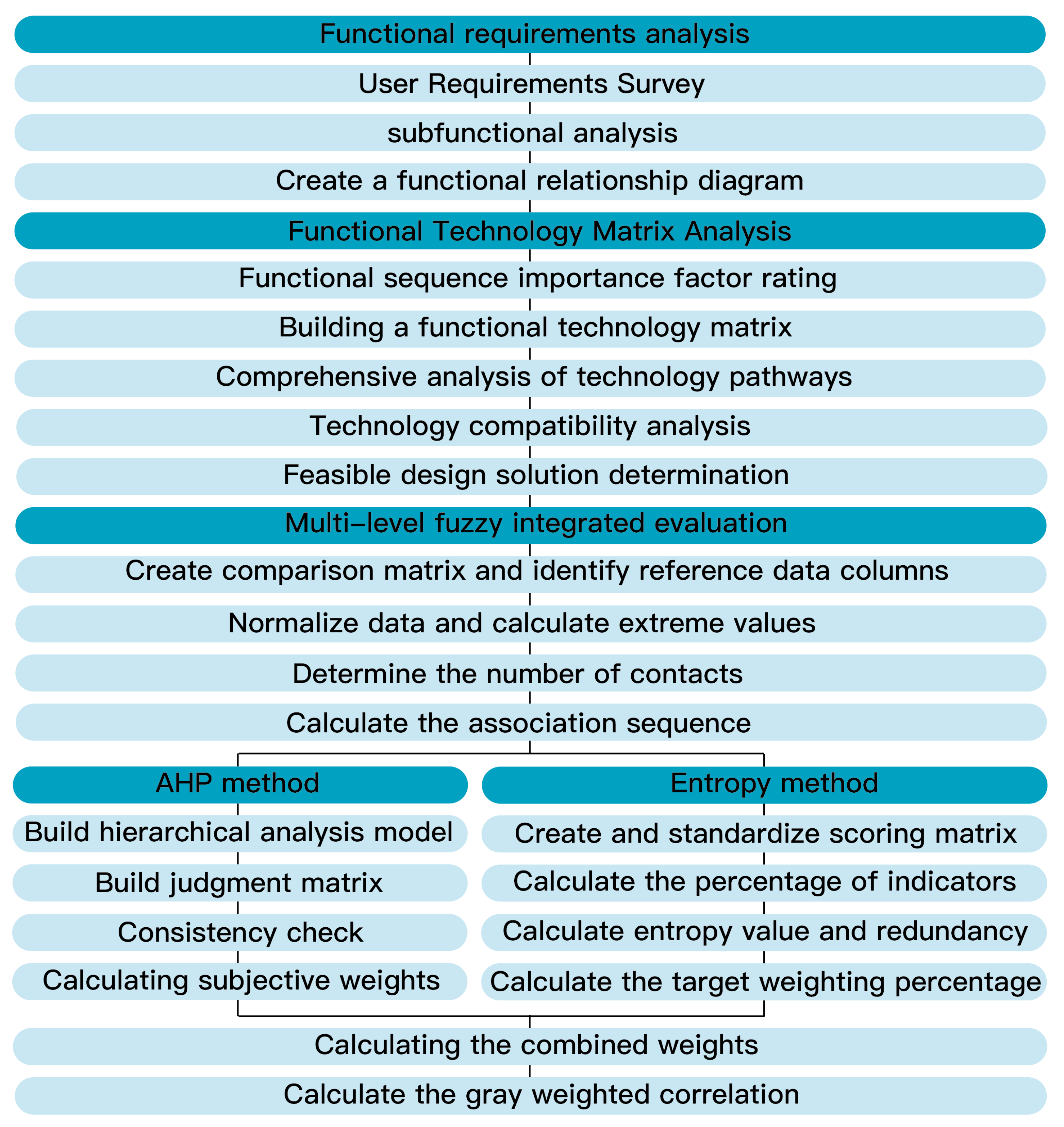
Figure 4.
Backrest modular massage program
Figure 5.
Modular rehabilitation program for the lower extremity
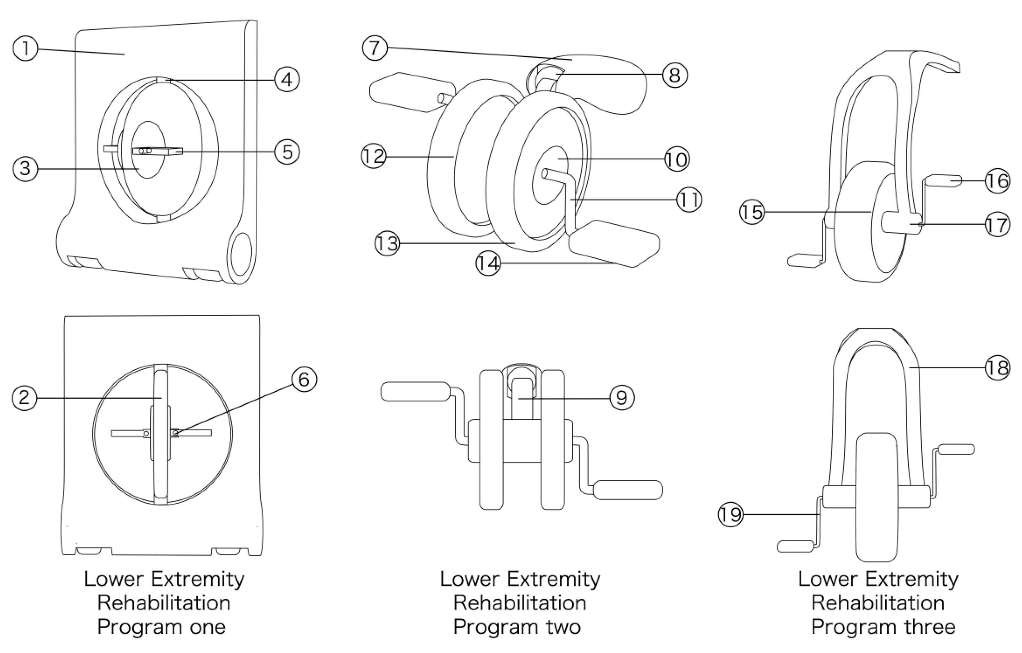
Figure 6.
Acupressure module solution
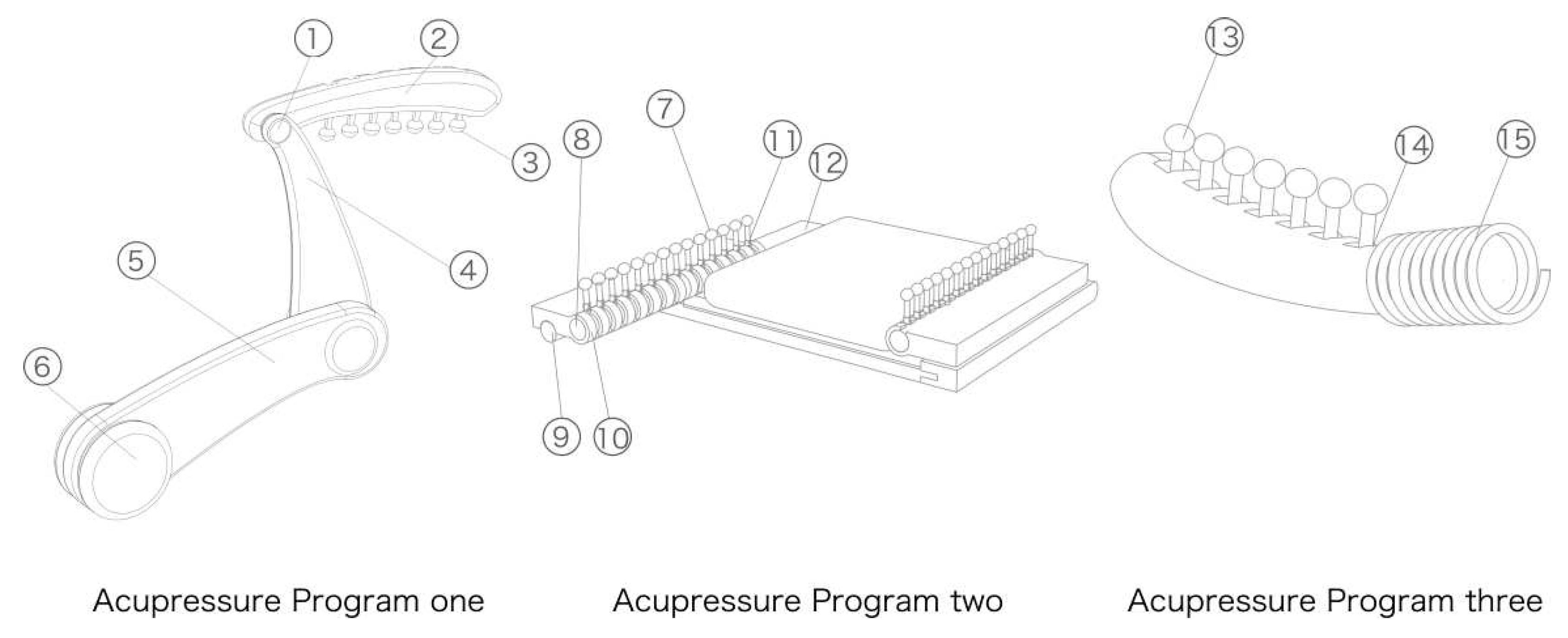
Figure 7.
Data Normalisation Matrix
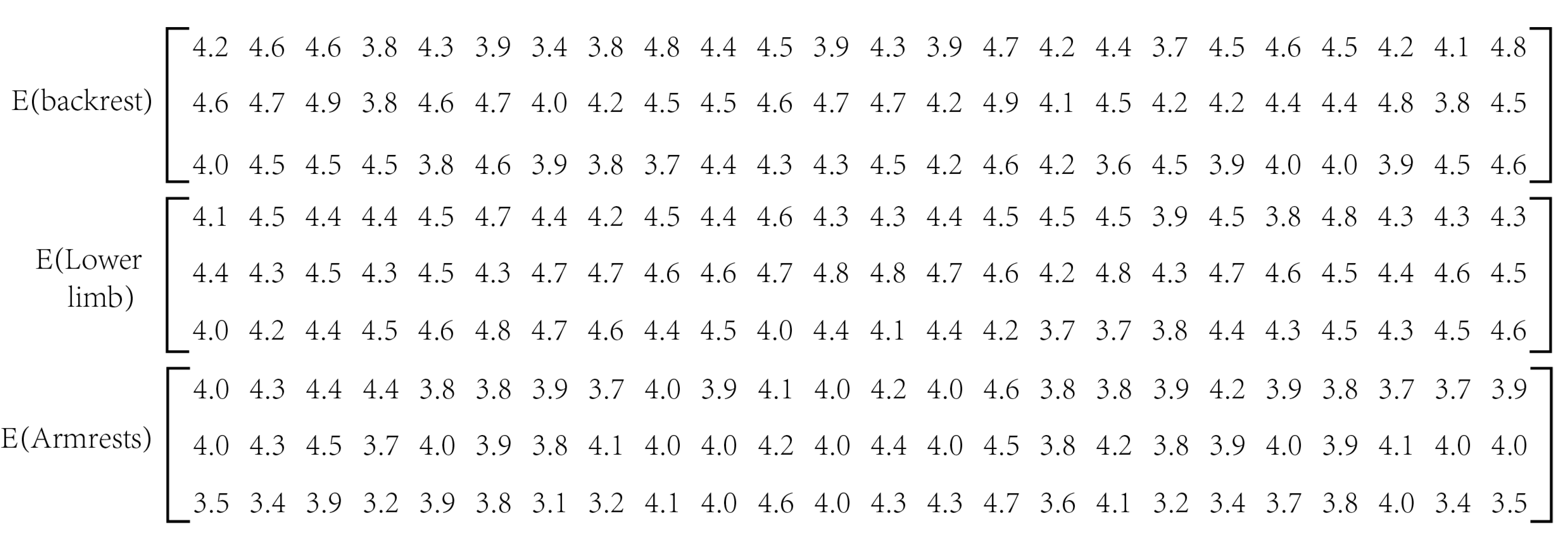
Figure 8.
Rehabilitation chair combination programme 1.
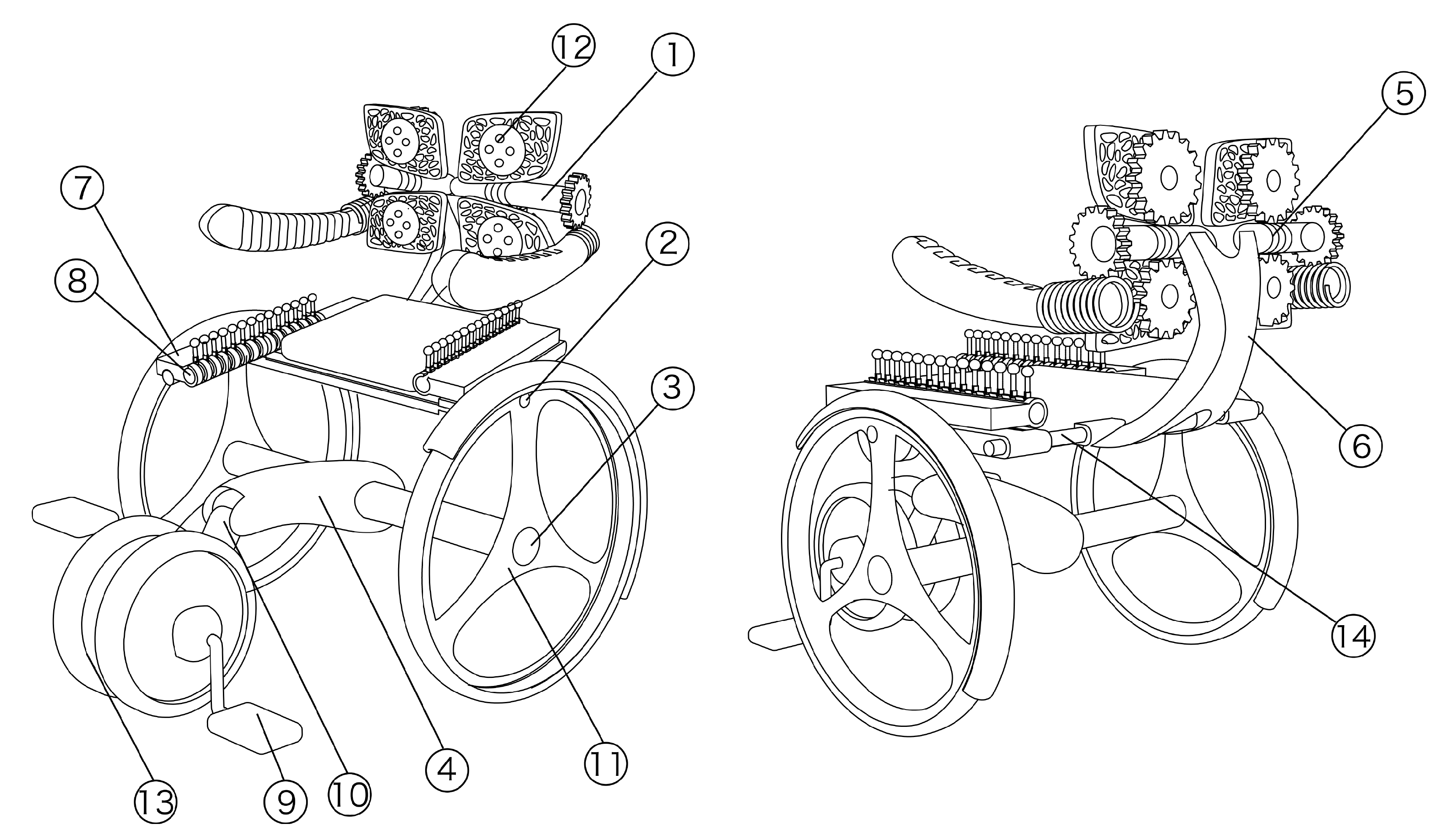
Figure 9.
Rehabilitation chair combination programme 2.
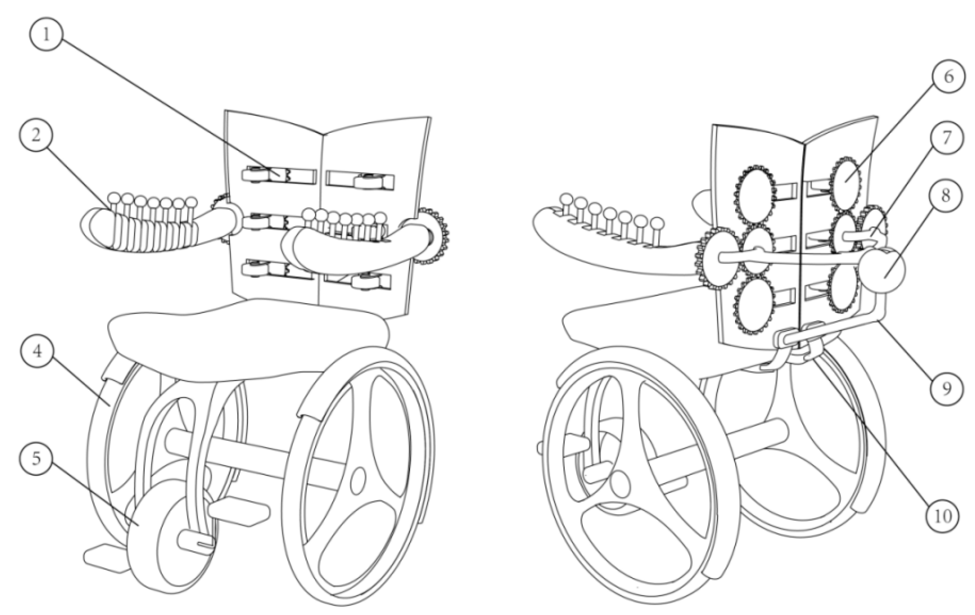
Figure 10.
This is a figure. Schemes follow the same formatting.
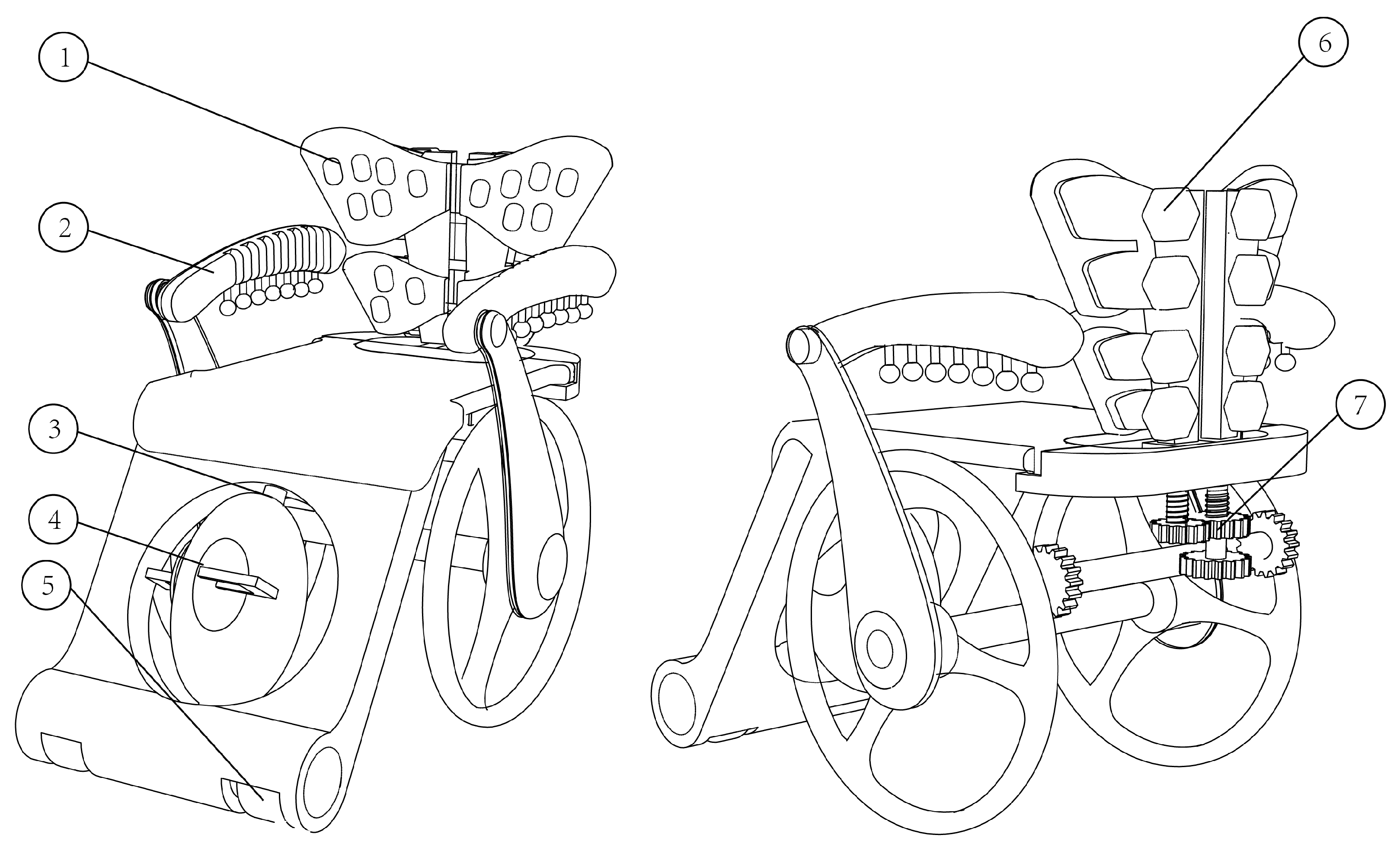
Figure 11.
Radar chart for programme evaluation
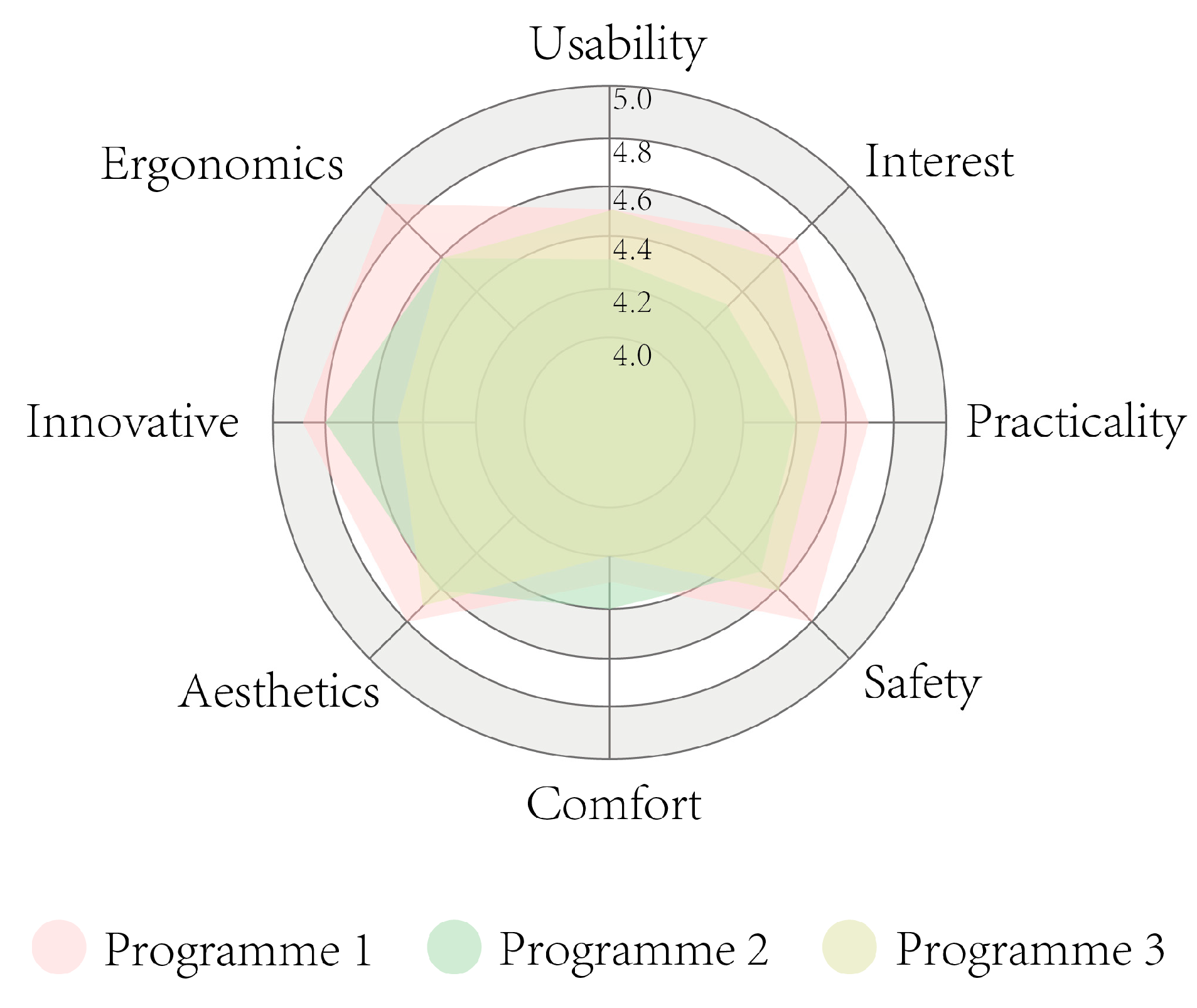
Figure 12.
Effect of rehabilitation chair
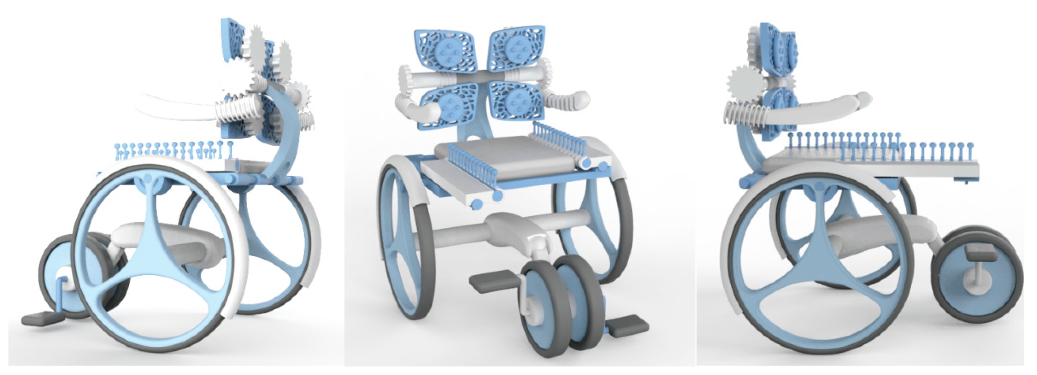
Table 1.
Functional technology matrix.
| Functions | Technology Pathways | ||||
|---|---|---|---|---|---|
| F1 | T1(1) | T1(2) | T1(1) | ... | T1(1) |
| F2 | T2(1) | T2(2) | T2(1) | ... | T1(1) |
| F3 | T3(1) | T3(2) | T3(1) | ... | T1(1) |
| F4 | T4(1) | T4(2) | T4(1) | ... | T1(1) |
| F5 | T5(1) | T5(2) | T5(1) | ... | T1(1) |
| F6 | T6(1) | T6(2) | T6(1) | ... | T1(1) |
| F7 | T7(1) | T7(2) | T7(1) | ... | T1(1) |
1 Tables may have a footer.
Table 2.
Rehabilitation Chair Functional Elements 0-4 Rating Scale.
| Functions | Coprime Comparison Scores | Function Importance Score | Functional Importance Factor | ||||||
|---|---|---|---|---|---|---|---|---|---|
| F1 | F2 | F3 | F4 | F5 | F6 | F7 | |||
| F1 | 0 | 3 | 2 | 3 | 2 | 3 | 2 | 15 | 0.174 |
| F2 | 1 | 0 | 1 | 3 | 1 | 2 | 3 | 11 | 0.130 |
| F3 | 2 | 3 | 0 | 3 | 2 | 3 | 2 | 15 | 0.174 |
| F4 | 1 | 1 | 1 | 0 | 1 | 2 | 1 | 7 | 0.081 |
| F5 | 2 | 3 | 2 | 3 | 0 | 3 | 2 | 15 | 0.174 |
| F6 | 1 | 2 | 1 | 2 | 1 | 0 | 1 | 8 | 0.093 |
| F7 | 2 | 1 | 2 | 3 | 2 | 3 | 0 | 15 | 0.174 |
| Total | 86 | 1 | |||||||
* Tables may have a footer.
Table 3.
Rehabilitation chair functional technology matrix.
| Functions | Technology Pathways | ||
|---|---|---|---|
| F1 | Roller(T11) | Worm gear(T12) | Struts(T13) |
| F2 | Roller(T21) | Sleeve type expansion slider(T22) | Telescopic slider(T23) |
| F3 | Screw(T31) | Mandrel(T32) | chuck(T33) |
| F4 | Support piece(T41) | Rotating section(T42) | rotating telescopic part(T43) |
| F5 | Folded movable rod end(T51) | Locking ring(T52) | Retaining pin(T53) |
| F6 | Wooden knockout head(T61) | Support wheel(T62) | Hinge rod(T63) |
| F7 | Turntable(T71) | Connection plate(T72) | Foot pedal(T73) |
Table 4.
Evaluation of technicality index coefficients functional elements of rehabilitation chair.
| Functions | Coprime Comparison Scores | Technical Index Scores | Technical Index Factors | |||
|---|---|---|---|---|---|---|
| F1 | T11 | T12 | T13 | |||
| T11 | 0 | 2 | 3 | 5 | 0.42 | |
| T12 | 2 | 0 | 3 | 5 | 0.42 | |
| T13 | 1 | 1 | 0 | 2 | 0.17 | |
| F2 | T21 | T22 | T23 | |||
| T21 | 0 | 1 | 1 | 2 | 0.17 | |
| T22 | 3 | 0 | 2 | 5 | 0.17 | |
| T23 | 3 | 2 | 0 | 5 | 0.42 | |
| F3 | T31 | T32 | T33 | |||
| T31 | 0 | 2 | 3 | 5 | 0.42 | |
| T32 | 2 | 0 | 3 | 5 | 0.42 | |
| T33 | 1 | 1 | 0 | 2 | 0.17 | |
| F4 | T41 | T42 | T43 | |||
| T41 | 0 | 3 | 3 | 6 | 0.46 | |
| T42 | 2 | 0 | 3 | 5 | 0.38 | |
| T43 | 1 | 1 | 0 | 2 | 0.15 | |
| F5 | T51 | T52 | T53 | |||
| T51 | 0 | 2 | 2 | 4 | 0.33 | |
| T52 | 2 | 0 | 3 | 5 | 0.42 | |
| T53 | 2 | 1 | 0 | 3 | 0.25 | |
| F6 | T61 | T62 | T63 | |||
| T61 | 0 | 2 | 1 | 3 | 0.25 | |
| T62 | 2 | 0 | 2 | 4 | 0.33 | |
| T63 | 1 | 2 | 0 | 5 | 0.42 | |
| F7 | T71 | T72 | T73 | |||
| T71 | 0 | 2 | 2 | 4 | 0.25 | |
| T72 | 2 | 0 | 2 | 4 | 0.25 | |
| T73 | 2 | 2 | 0 | 4 | 0.25 | |
Table 5.
Evaluation of environmental protection index coefficients of functional elements of rehabilitation chair.
Table 5.
Evaluation of environmental protection index coefficients of functional elements of rehabilitation chair.
| Functions | Coprime Comparison Scores | Technical Index Scores | Technical Index Factors | |||
|---|---|---|---|---|---|---|
| F1 | T11 | T12 | T13 | |||
| T11 | 0 | 2 | 1 | 3 | 0.25 | |
| T12 | 2 | 0 | 1 | 3 | 0.25 | |
| T13 | 3 | 3 | 0 | 6 | 0.50 | |
| F2 | T21 | T22 | T23 | |||
| T21 | 0 | 3 | 1 | 4 | 0.33 | |
| T22 | 1 | 0 | 1 | 2 | 0.17 | |
| T23 | 3 | 3 | 0 | 6 | 0.50 | |
| F3 | T31 | T32 | T33 | |||
| T31 | 0 | 2 | 3 | 5 | 0.42 | |
| T32 | 2 | 0 | 3 | 5 | 0.42 | |
| T33 | 1 | 1 | 0 | 2 | 0.16 | |
| F4 | T41 | T42 | T43 | |||
| T41 | 0 | 2 | 3 | 5 | 0.42 | |
| T42 | 2 | 0 | 3 | 5 | 0.42 | |
| T43 | 1 | 1 | 0 | 2 | 0.16 | |
| F5 | T51 | T52 | T53 | |||
| T51 | 0 | 3 | 1 | 4 | 0.33 | |
| T52 | 1 | 0 | 1 | 2 | 0.17 | |
| T53 | 3 | 3 | 0 | 6 | 0.50 | |
| F6 | T61 | T62 | T63 | |||
| T61 | 0 | 2 | 3 | 5 | 0.42 | |
| T62 | 2 | 0 | 3 | 5 | 0.42 | |
| T63 | 1 | 1 | 0 | 2 | 0.16 | |
| F7 | T71 | T72 | T73 | |||
| T71 | 0 | 3 | 2 | 5 | 0.42 | |
| T72 | 1 | 0 | 1 | 2 | 0.16 | |
| T73 | 2 | 3 | 0 | 5 | 0.42 | |
Table 6.
Evaluation of applicability index coefficients of functional elements of modular rehabilitation chair.
Table 6.
Evaluation of applicability index coefficients of functional elements of modular rehabilitation chair.
| Functions | Coprime Comparison Scores | Technical Index Scores | Technical Index Factors | |||
|---|---|---|---|---|---|---|
| F1 | T11 | T12 | T13 | |||
| T11 | 0 | 2 | 3 | 5 | 0.42 | |
| T12 | 2 | 0 | 3 | 5 | 0.42 | |
| T13 | 1 | 1 | 0 | 2 | 0.16 | |
| F2 | T21 | T22 | T23 | |||
| T21 | 0 | 1 | 1 | 2 | 0.17 | |
| T22 | 3 | 0 | 3 | 6 | 0.50 | |
| T23 | 3 | 1 | 0 | 4 | 0.33 | |
| F3 | T31 | T32 | T33 | |||
| T31 | 0 | 1 | 3 | 4 | 0.33 | |
| T32 | 3 | 0 | 3 | 6 | 0.50 | |
| T33 | 1 | 1 | 0 | 2 | 0.17 | |
| F4 | T41 | T42 | T43 | |||
| T41 | 0 | 3 | 3 | 6 | 0.50 | |
| T42 | 1 | 0 | 3 | 4 | 0.33 | |
| T43 | 1 | 1 | 0 | 2 | 0.17 | |
| F5 | T51 | T52 | T53 | |||
| T51 | 0 | 3 | 2 | 5 | 0.45 | |
| T52 | 1 | 0 | 1 | 2 | 0.18 | |
| T53 | 2 | 3 | 0 | 4 | 0.36 | |
| F6 | T61 | T62 | T63 | |||
| T61 | 0 | 1 | 2 | 3 | 0.23 | |
| T62 | 3 | 0 | 2 | 5 | 0.38 | |
| T63 | 3 | 2 | 0 | 5 | 0.38 | |
| F7 | T71 | T72 | T73 | |||
| T71 | 0 | 3 | 2 | 5 | 0.42 | |
| T72 | 1 | 0 | 1 | 2 | 0.16 | |
| T73 | 2 | 3 | 0 | 5 | 0.42 | |
Table 7.
Technical compatibility scoring matrix.
| Feasibility | ||||
| T1(1) | T1(2) | ... | T1(n) | |
| T1(1) | 0/1 | 0/1 | ... | 0/1 |
| T1(2) | 0/1 | 0/1 | ... | 0/1 |
| ... | ... | ... | ... | ... |
| T1(n) | 0/1 | 0/1 | ... | 0/1 |
Table 8.
One to Nine Scaling method
| Scale | Implication |
| 1 | By comparison, the two elements are equally important. |
| 3 | By comparison, one element is slightly more important than the other. |
| 5 | By comparison, one element is obviously more important than the other. |
| 7 | By comparison, one element is strongly more important than the other. |
| 9 | By comparison, one element is extremely more important than the other. |
| 2,4,6,8 | The middle value between each of the above two adjacent scales. |
Table 13.
Calculation results of comprehensive weights.
| E1 | E11 | E12 | E13 | E14 |
| C1 | 0.32034 | 0.16742 | 0.38398 | 0.12826 |
| E | E21 | E22 | E23 | E24 |
| C | 0.34191 | 0.18659 | 0.35339 | 0.11812 |
| E | E31 | E32 | E33 | E34 |
| C | 0.14431 | 0.21168 | 0.46171 | 0.33998 |
| E | E41 | E42 | E43 | E44 |
| C | 0.08329 | 0.48331 | 0.25168 | 0.09982 |
| E | E51 | E52 | E53 | E54 |
| C | 0.13216 | 0.11639 | 0.34902 | 0.32594 |
| E | E61 | E62 | E63 | E64 |
| C | 0.31501 | 0.39758 | 0.12033 | 0.16704 |
1 E for Evaluation Indicators;C for Composite Weights.
Table 14.
Grey integrated weight correlation and its ranking
| Programs | Backrest 1 | Backrest 2 | Backrest 3 | Lower Limb1 | Lower Limb2 | Lower Limb3 | Handrail 1 | Handrail 2 | Handrail 3 |
|---|---|---|---|---|---|---|---|---|---|
| Relevance | 0.182 | 0.188 | 0.177 | 0.171 | 0.178 | 0.173 | 0.175 | 0.192 | 0.185 |
| Ranking | 2 | 1 | 3 | 3 | 1 | 2 | 3 | 1 | 2 |
Disclaimer/Publisher’s Note: The statements, opinions and data contained in all publications are solely those of the individual author(s) and contributor(s) and not of MDPI and/or the editor(s). MDPI and/or the editor(s) disclaim responsibility for any injury to people or property resulting from any ideas, methods, instructions or products referred to in the content. |
© 2023 by the authors. Licensee MDPI, Basel, Switzerland. This article is an open access article distributed under the terms and conditions of the Creative Commons Attribution (CC BY) license (http://creativecommons.org/licenses/by/4.0/).
Copyright: This open access article is published under a Creative Commons CC BY 4.0 license, which permit the free download, distribution, and reuse, provided that the author and preprint are cited in any reuse.


