Submitted:
27 September 2023
Posted:
28 September 2023
You are already at the latest version
Abstract
Keywords:
1. Introduction
1.1. An Overview of Twitter: a Globally Popular Social Media Platform
1.2. Exoskeleton Technology and its Emergence: A Brief Overview
2. Literature Review
3.1. Review of Analysis of Tweets focusing on different Industries and Interdisciplinary Research
3.2. Review of Analysis of Tweets focusing on Robotics and Wearable Robotics-based Technologies
3. Methodology
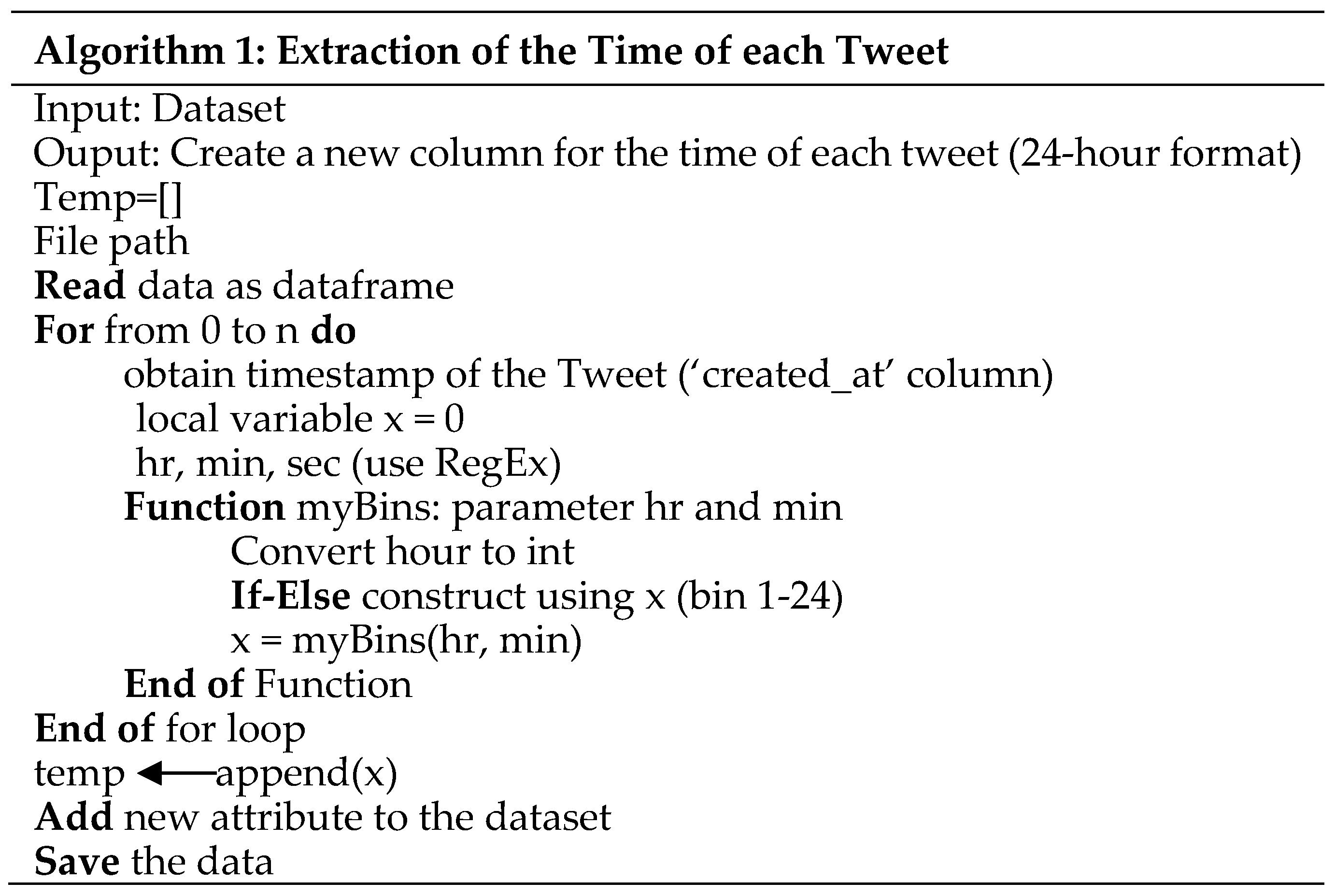 |
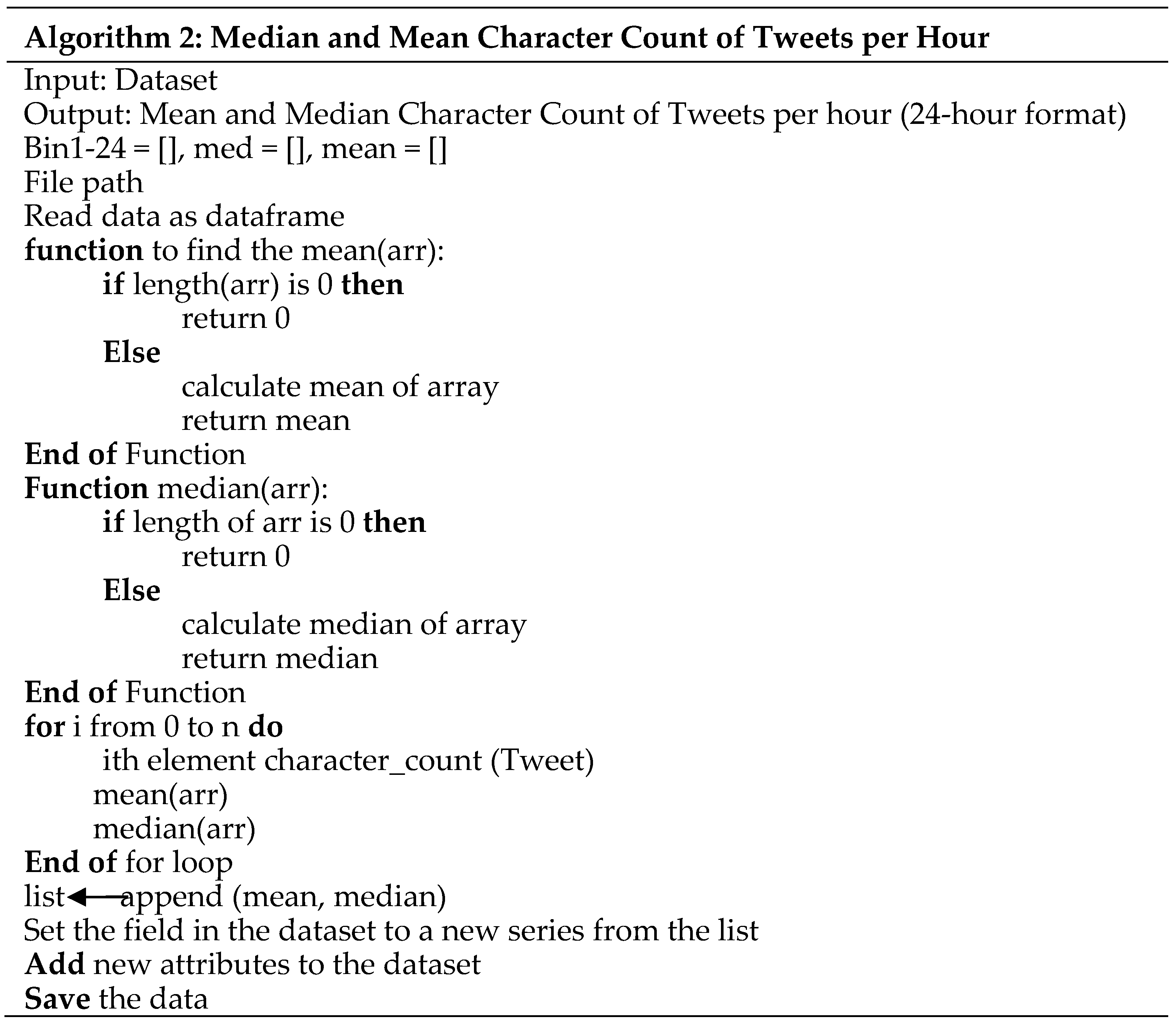 |
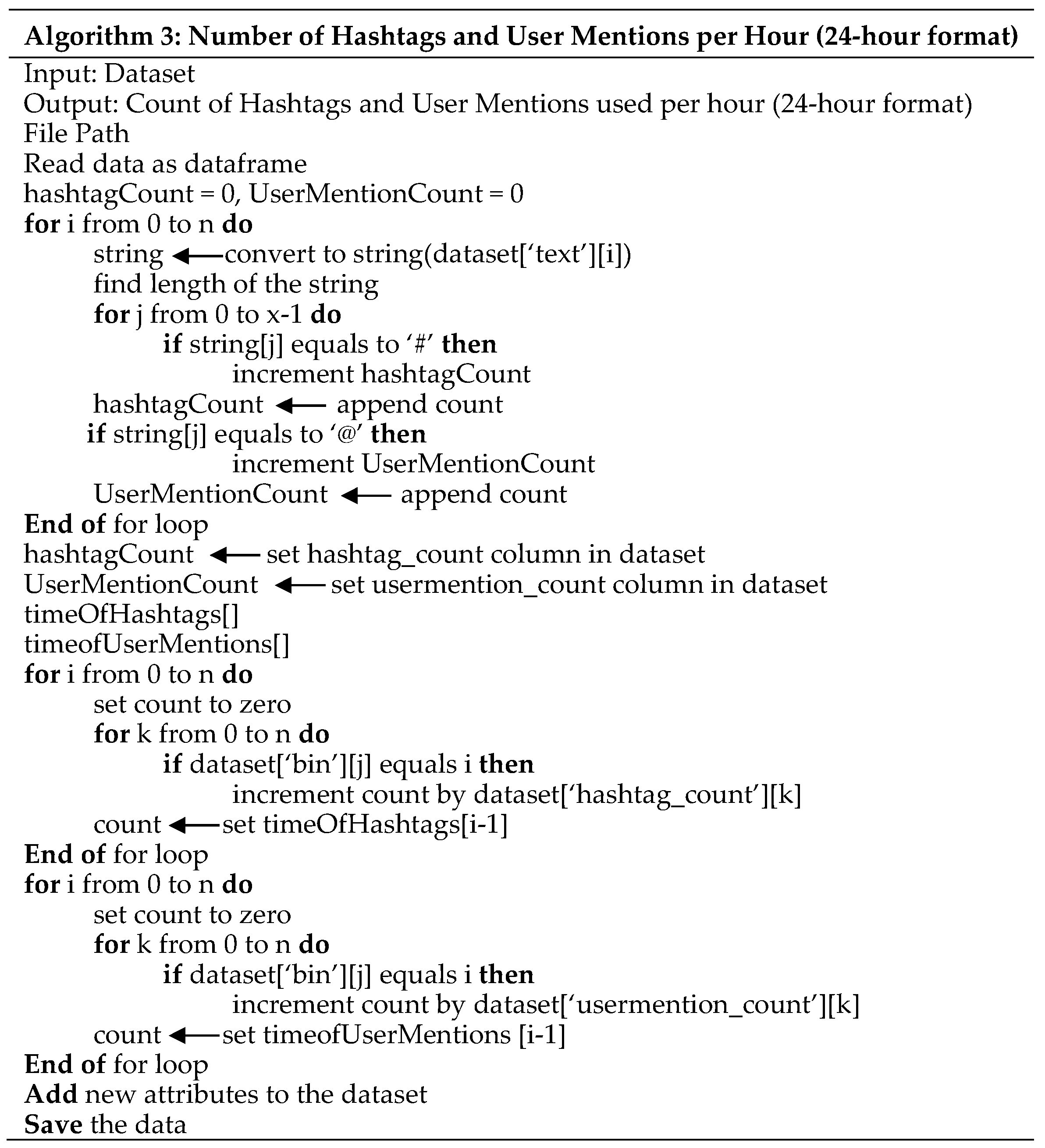 |
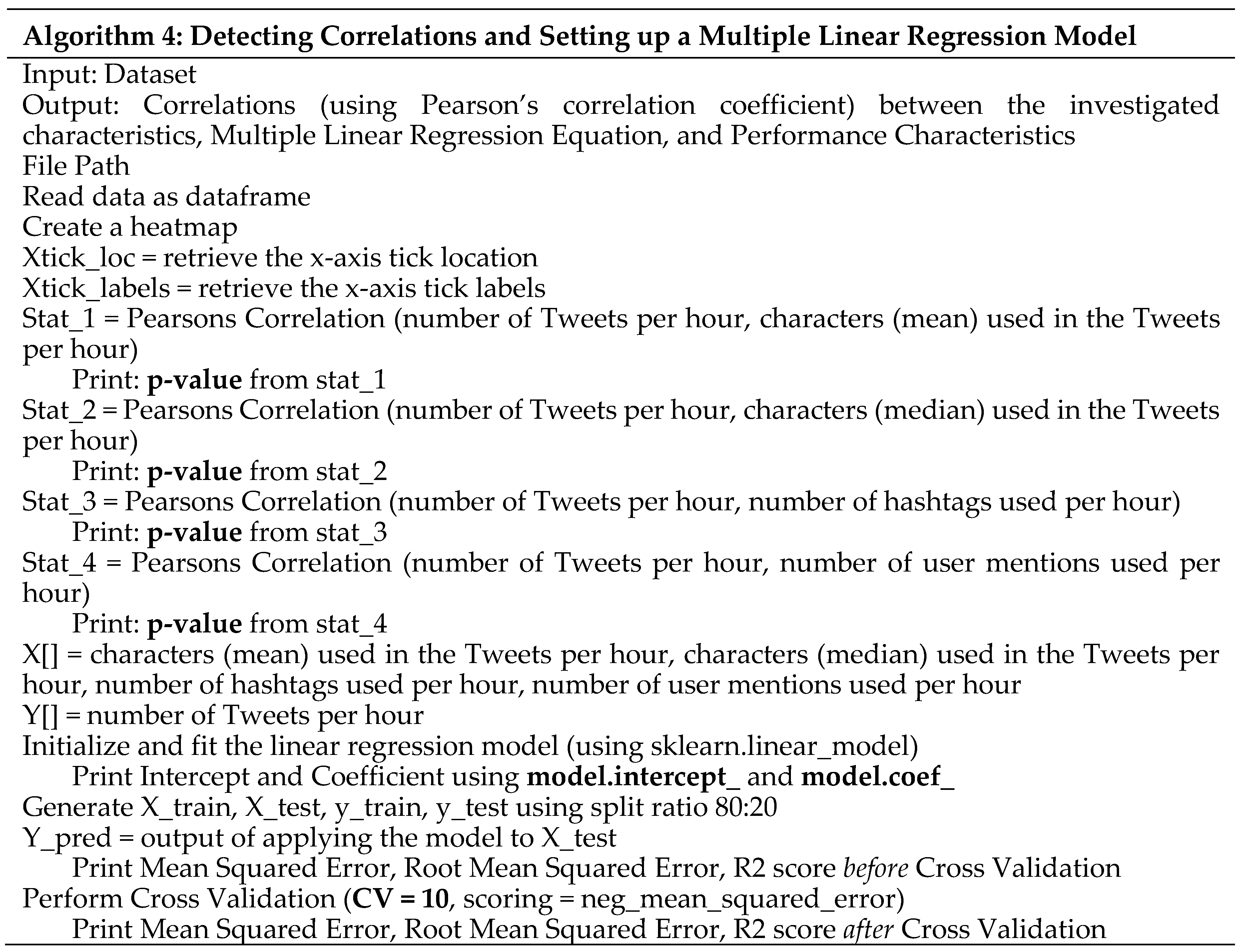 |
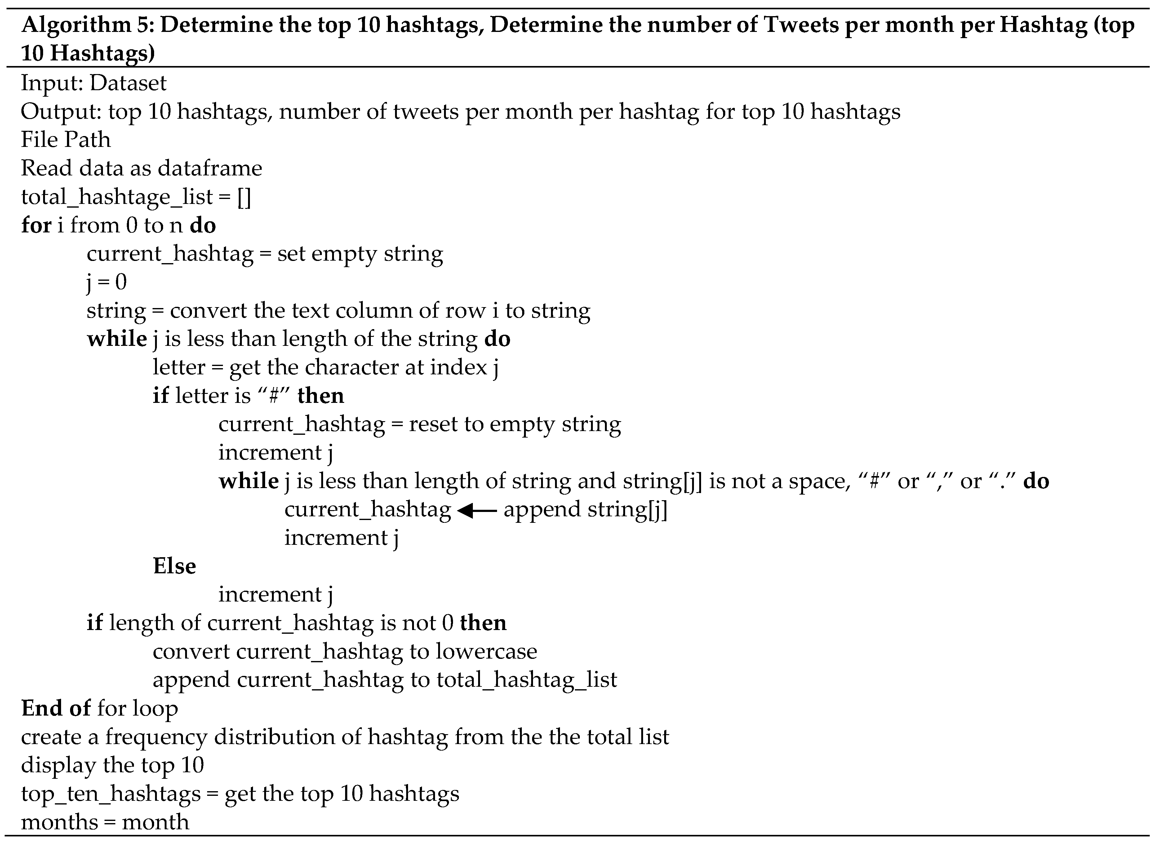 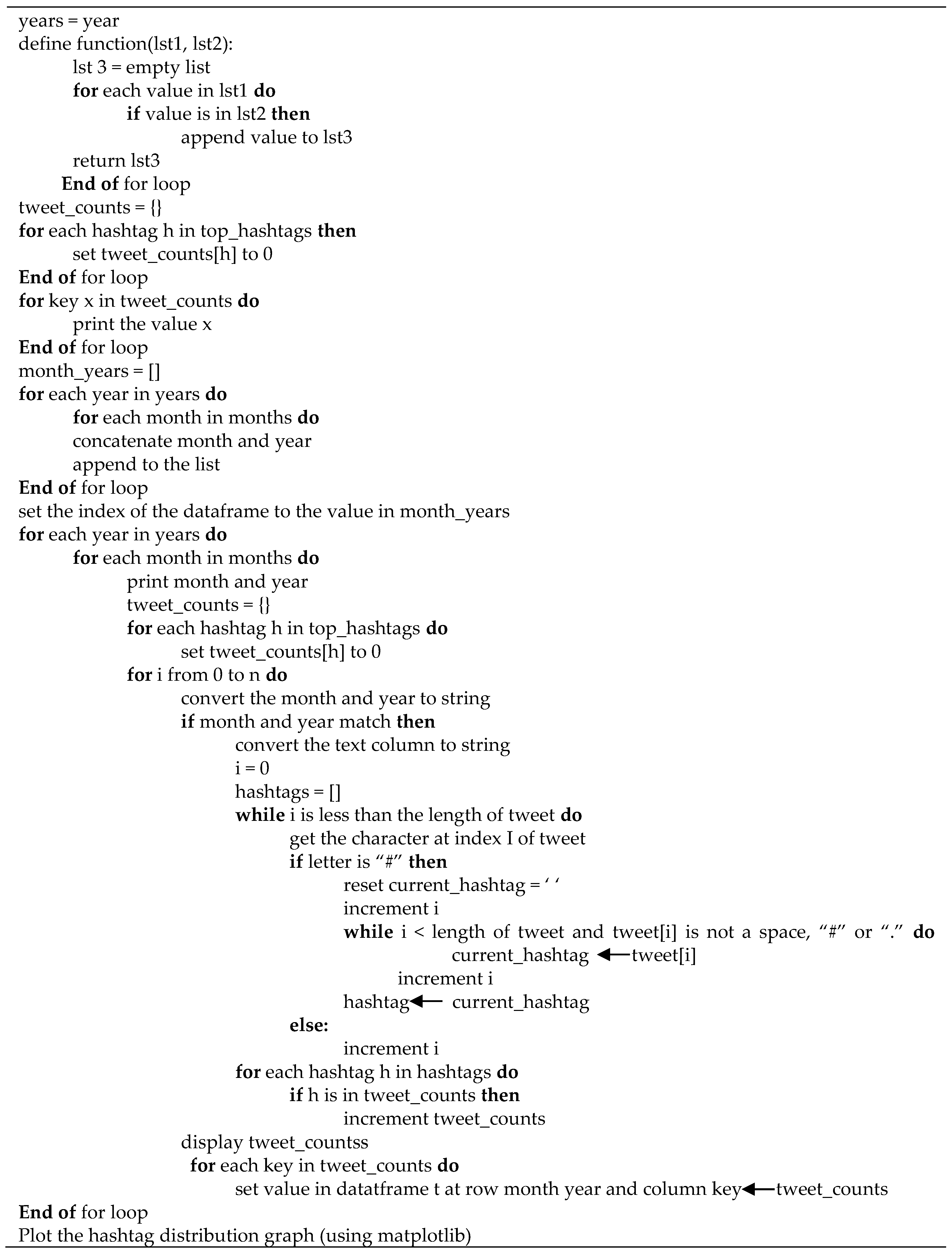
|
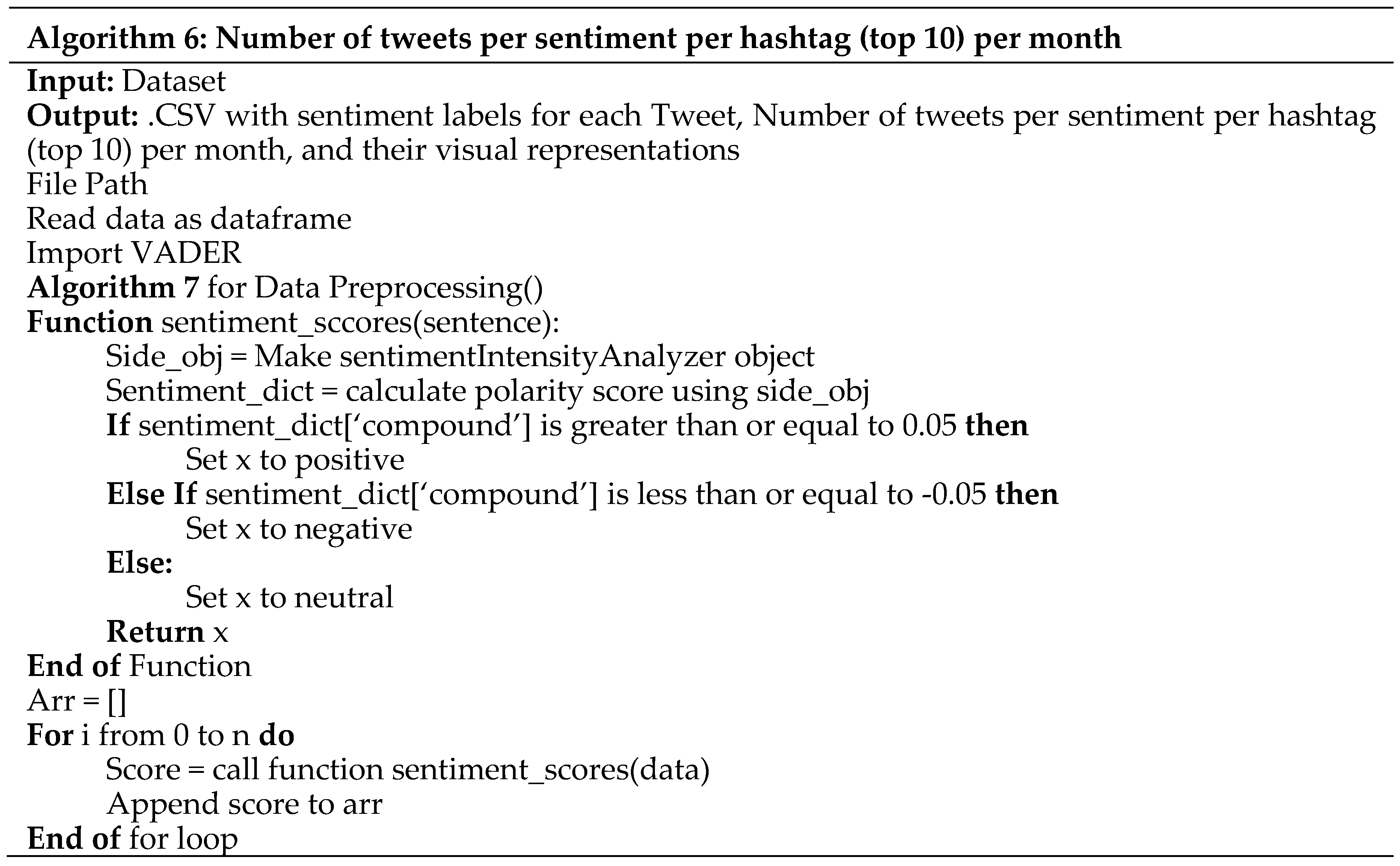 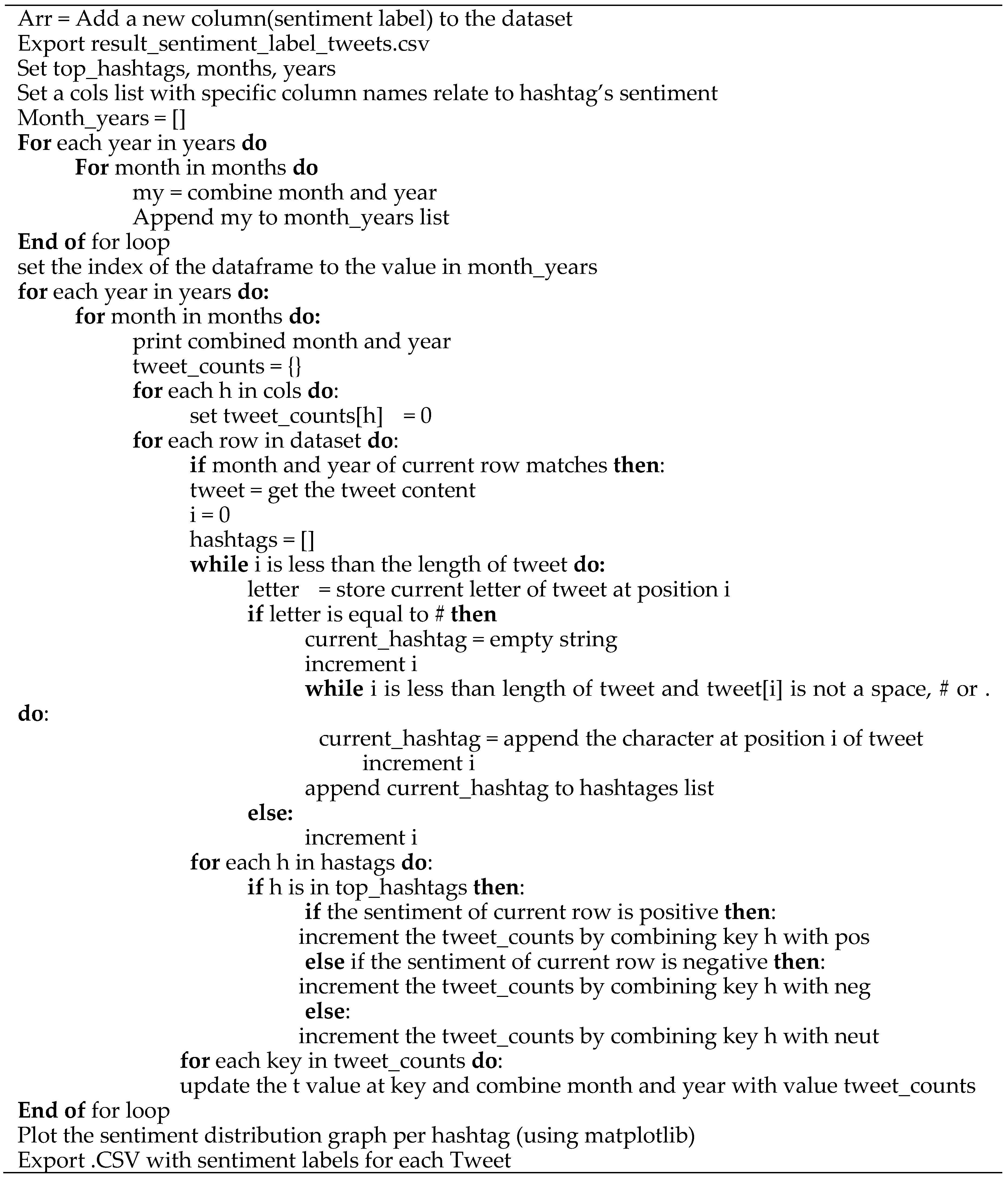
|
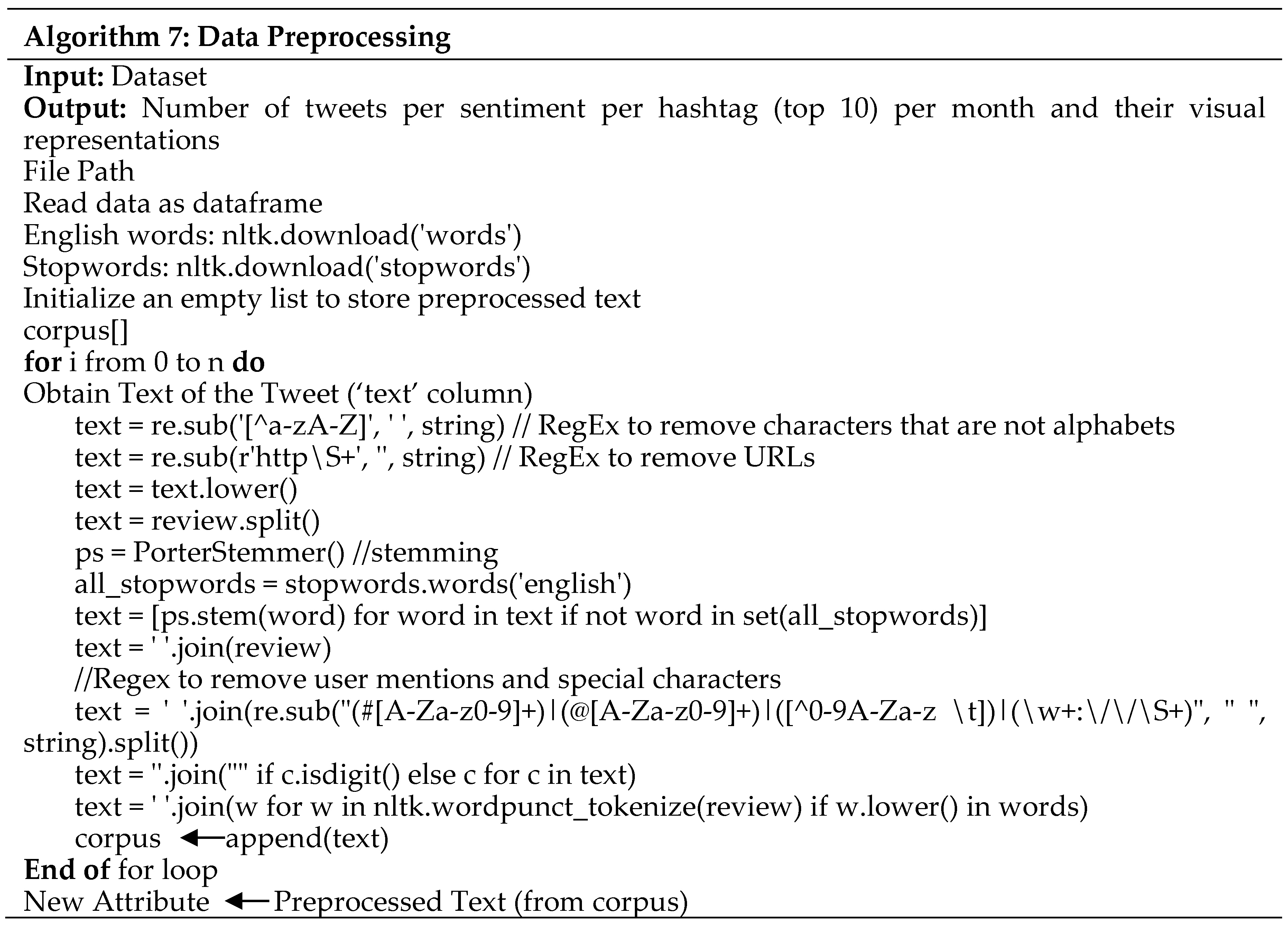 |
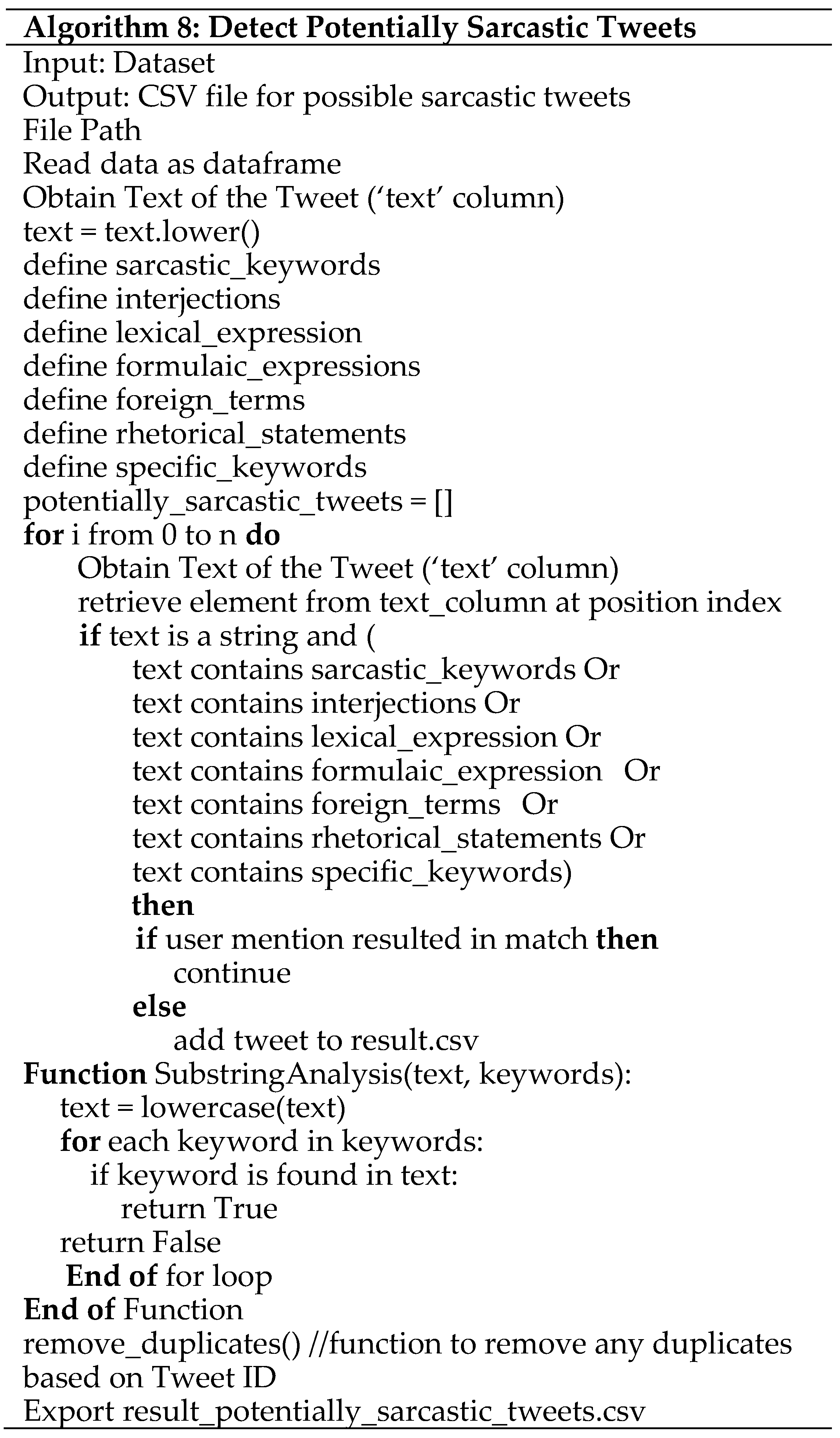 |
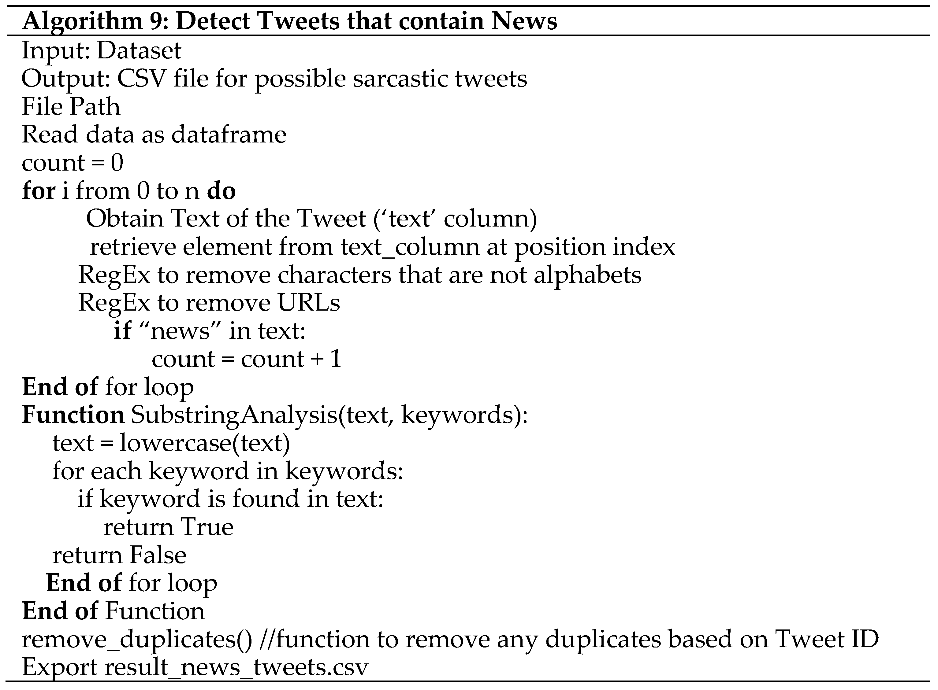 |
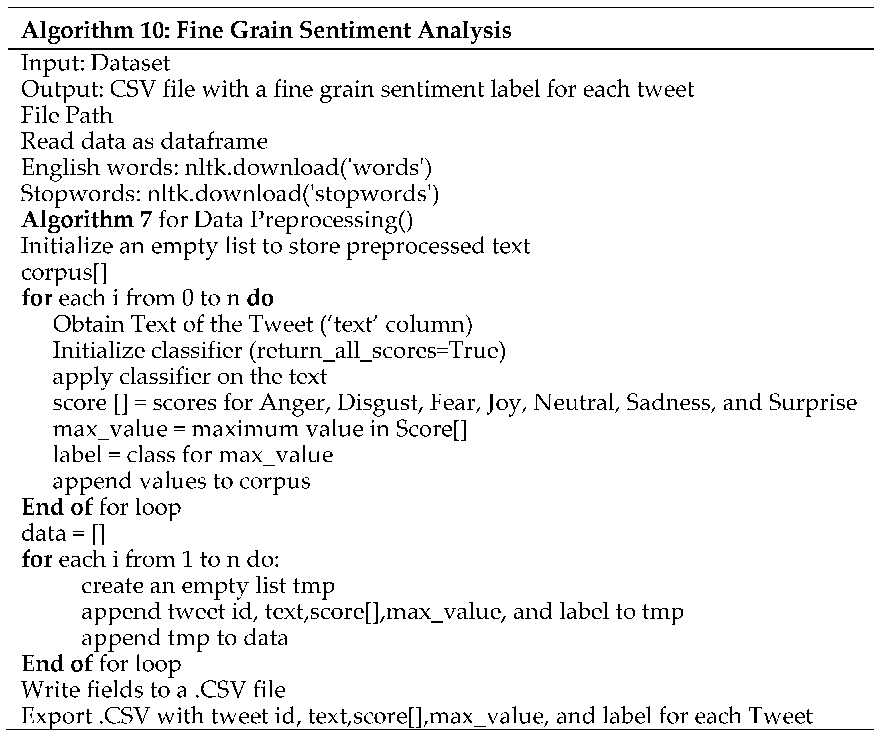 |
4. Results and Discussions
- a)
- number of Tweets per hour and number of characters (mean value) in the Tweets per hour
- b)
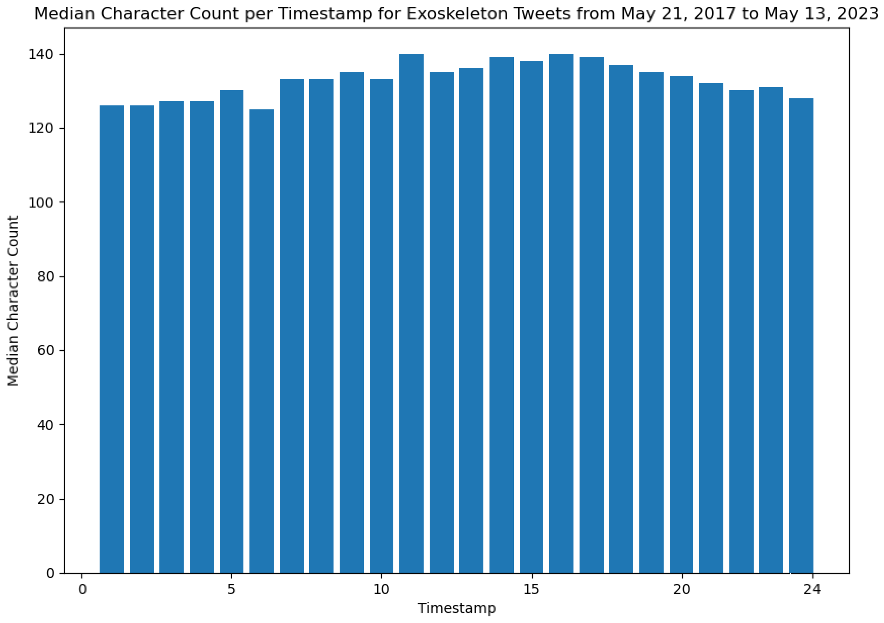
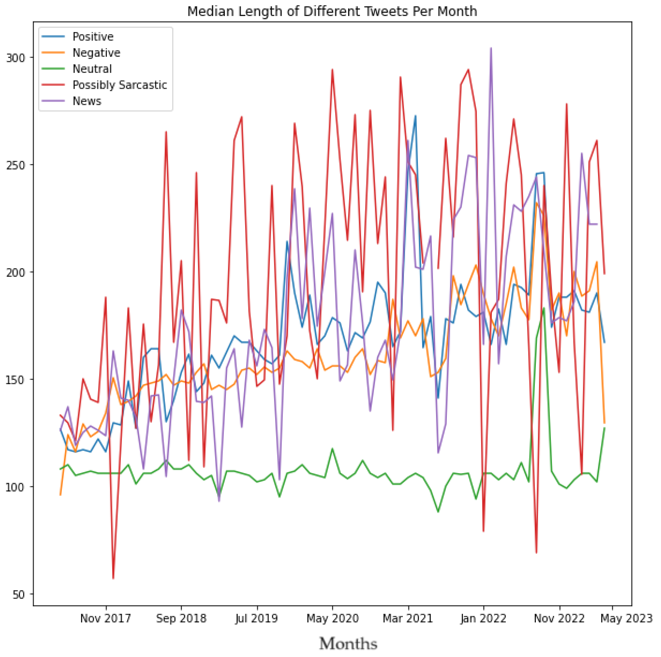
- number of Tweets per hour and number of characters (median value) in the Tweets per hour
- c)
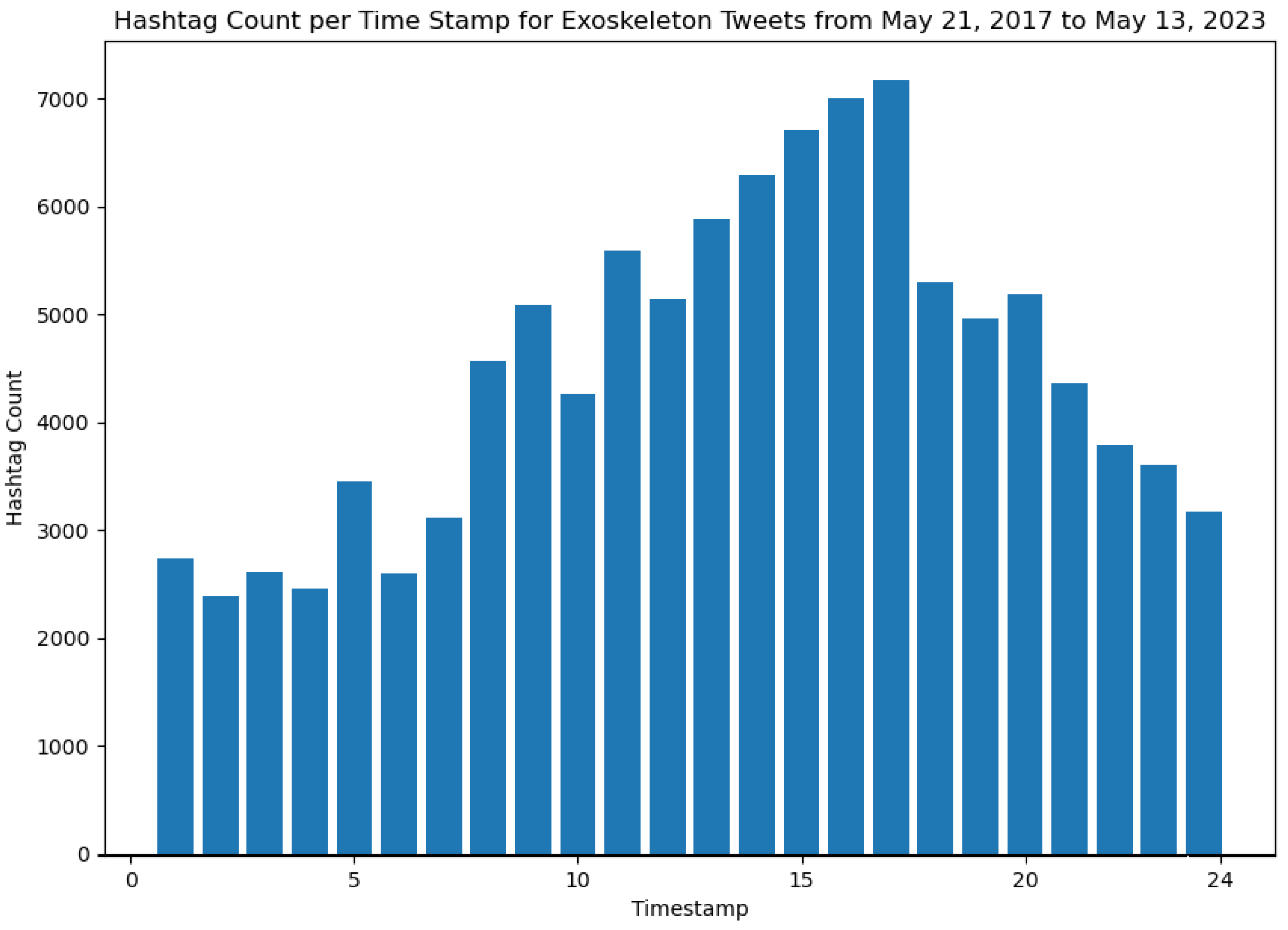
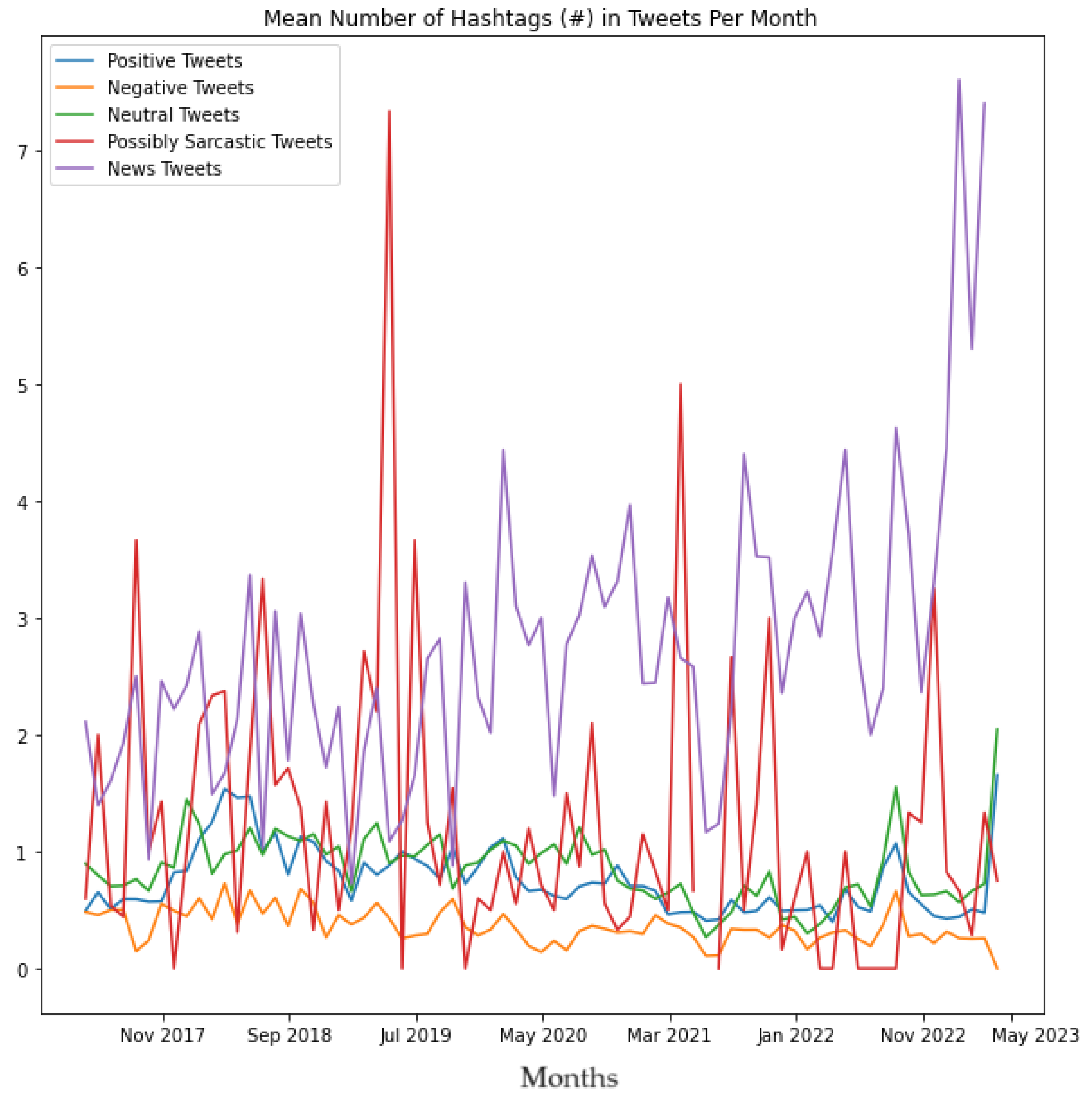
- number of Tweets per hour and number of hashtags in the Tweets per hour
- d)
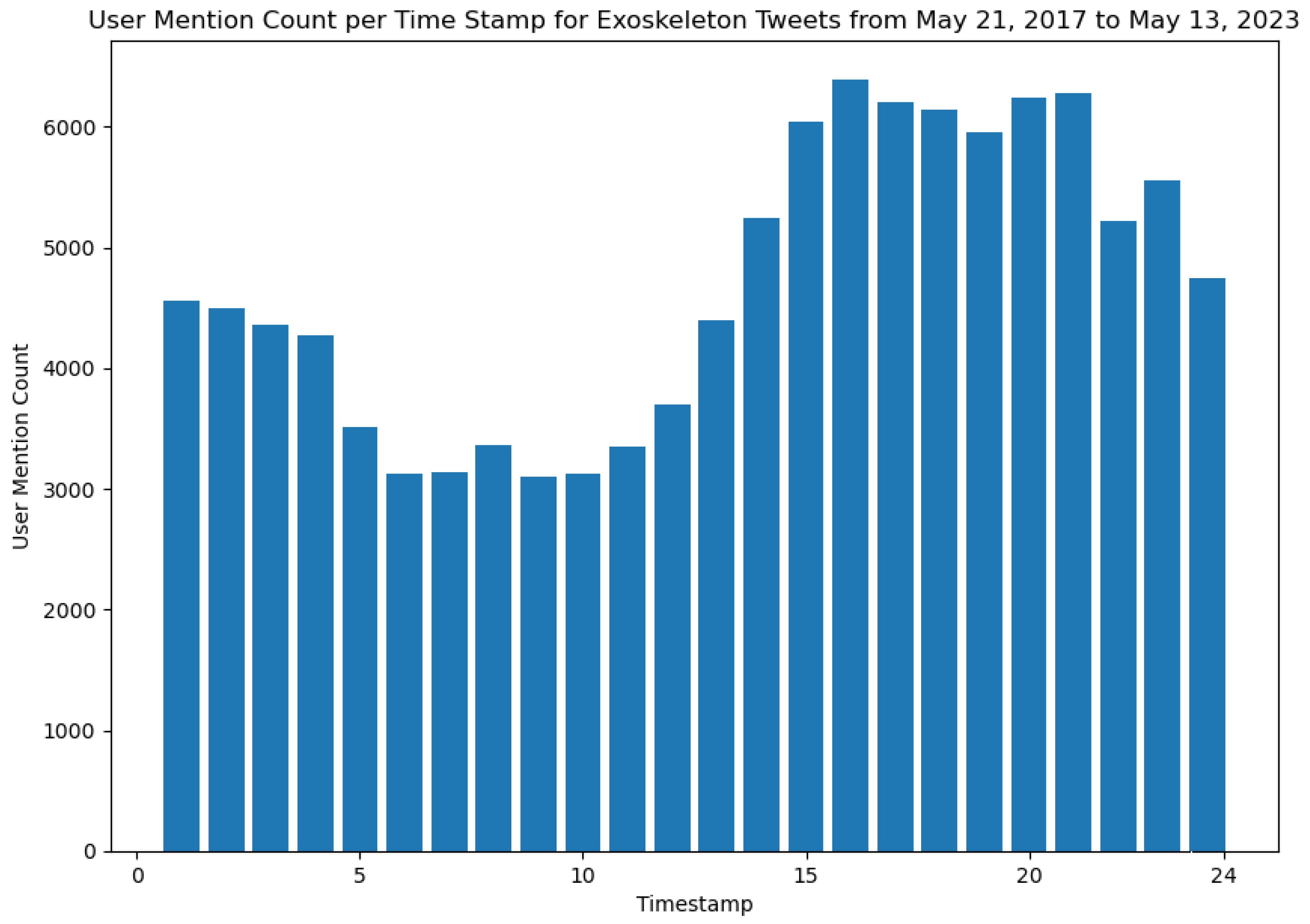
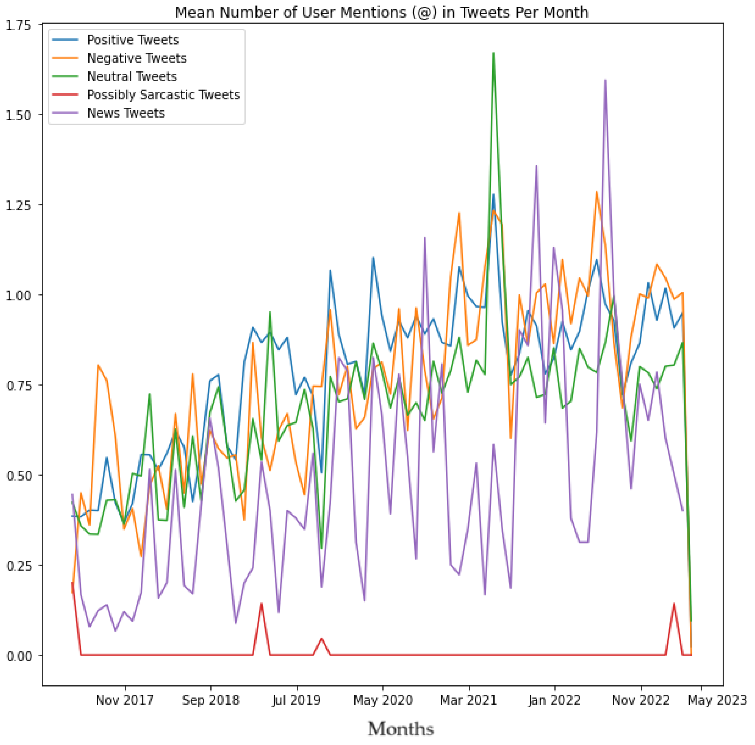
- number of Tweets per hour and number of user mentions in the Tweets per hour
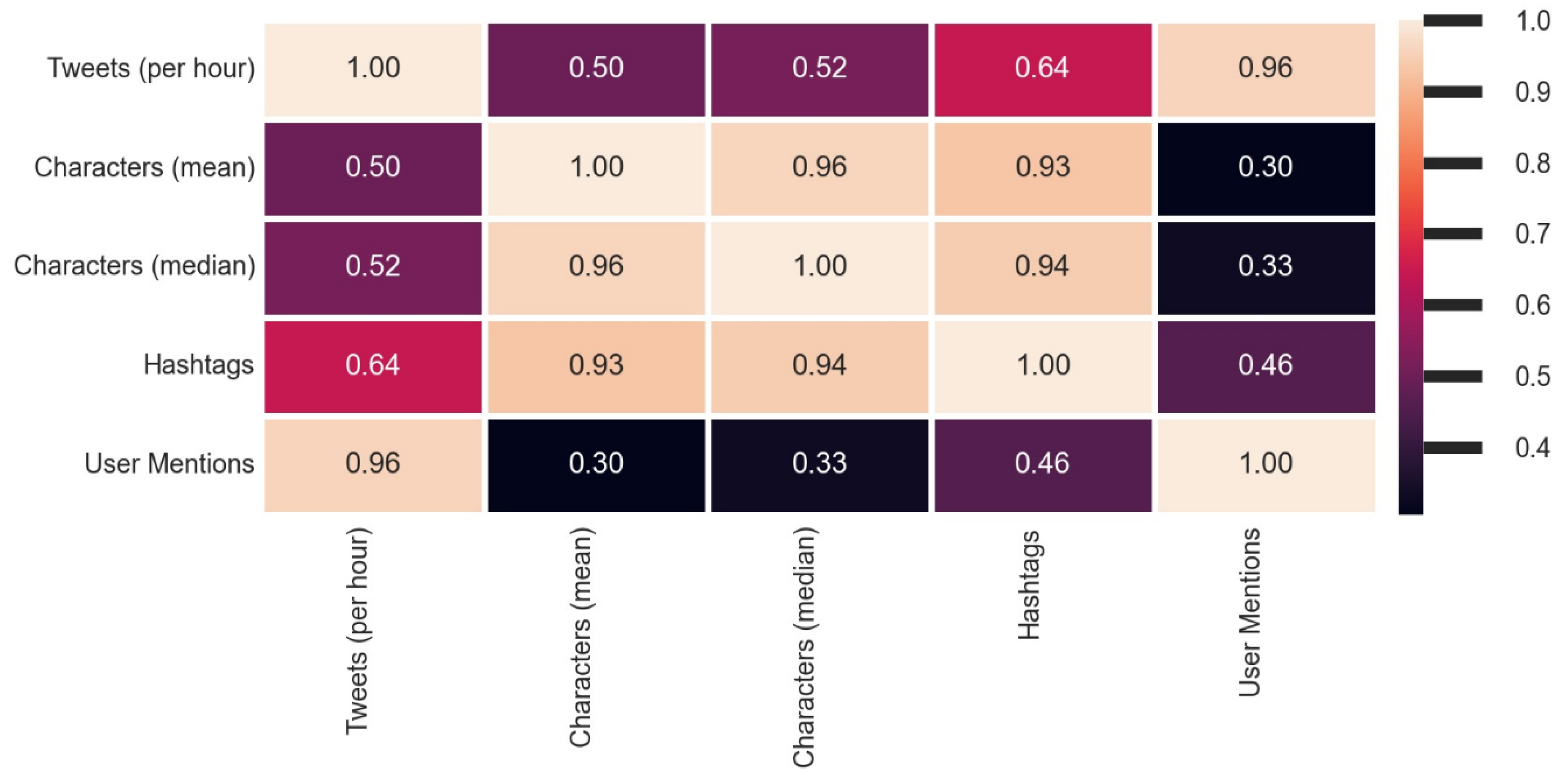
| Description | Value |
| Multiple Linear Regression Intercept | 2784.170988721279 |
| Multiple Linear Regression Coefficients | [11.78367763 -31.13336391 0.30537686 0.96967955] |
| R2 score | 0.9540953548345376 |
| Mean Squared Error (before cross-validation) | 54577.94142377716 |
| Root Mean Squared Error (before cross Validation) | 233.61922314693447 |
| Value of k for k-folds cross-validation | 10 |
| Mean Squared Error (after cross-validation) | 65260.27219328486 |
| Root Mean Squared Error (after cross-validation) | 255.46090149626588 |
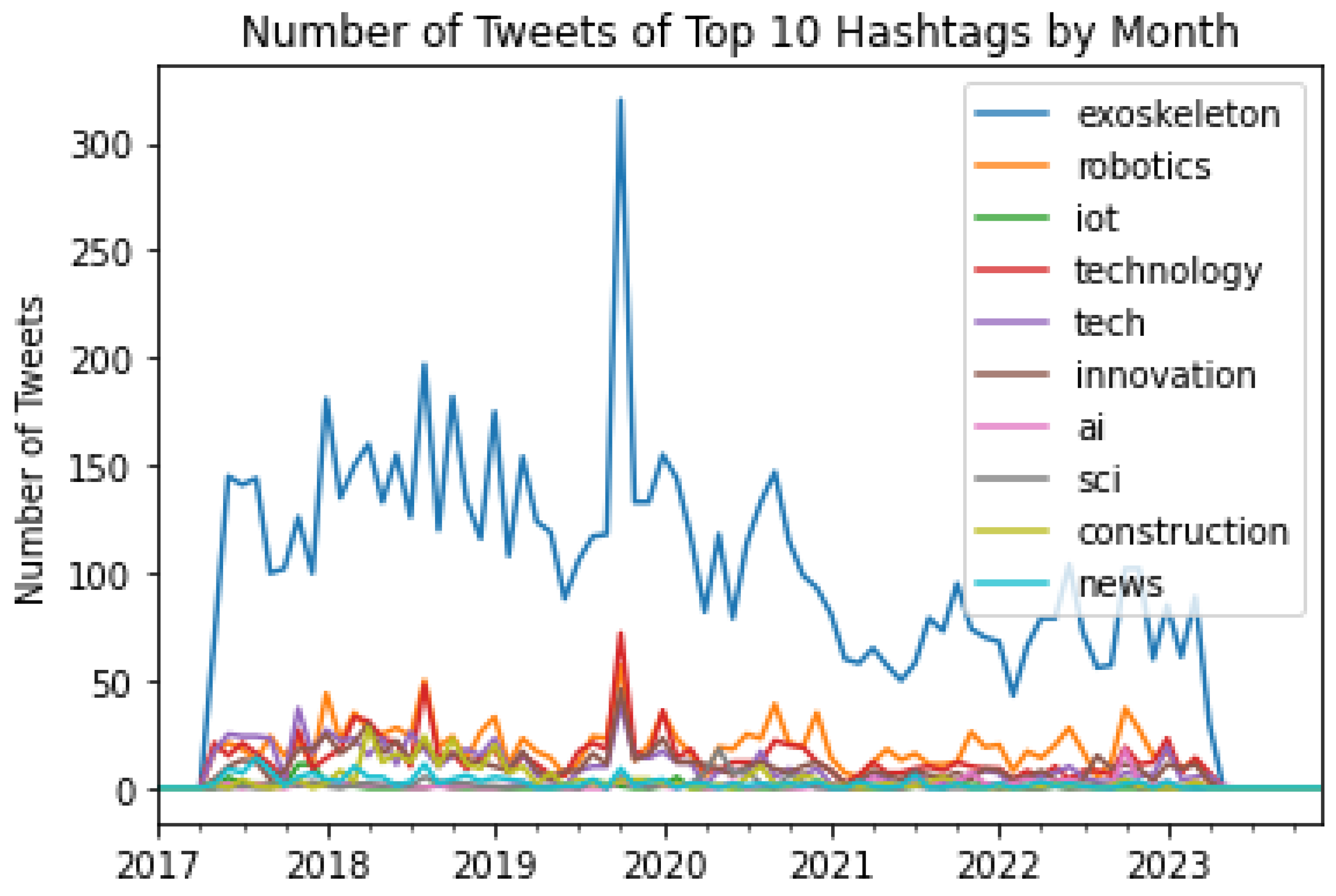
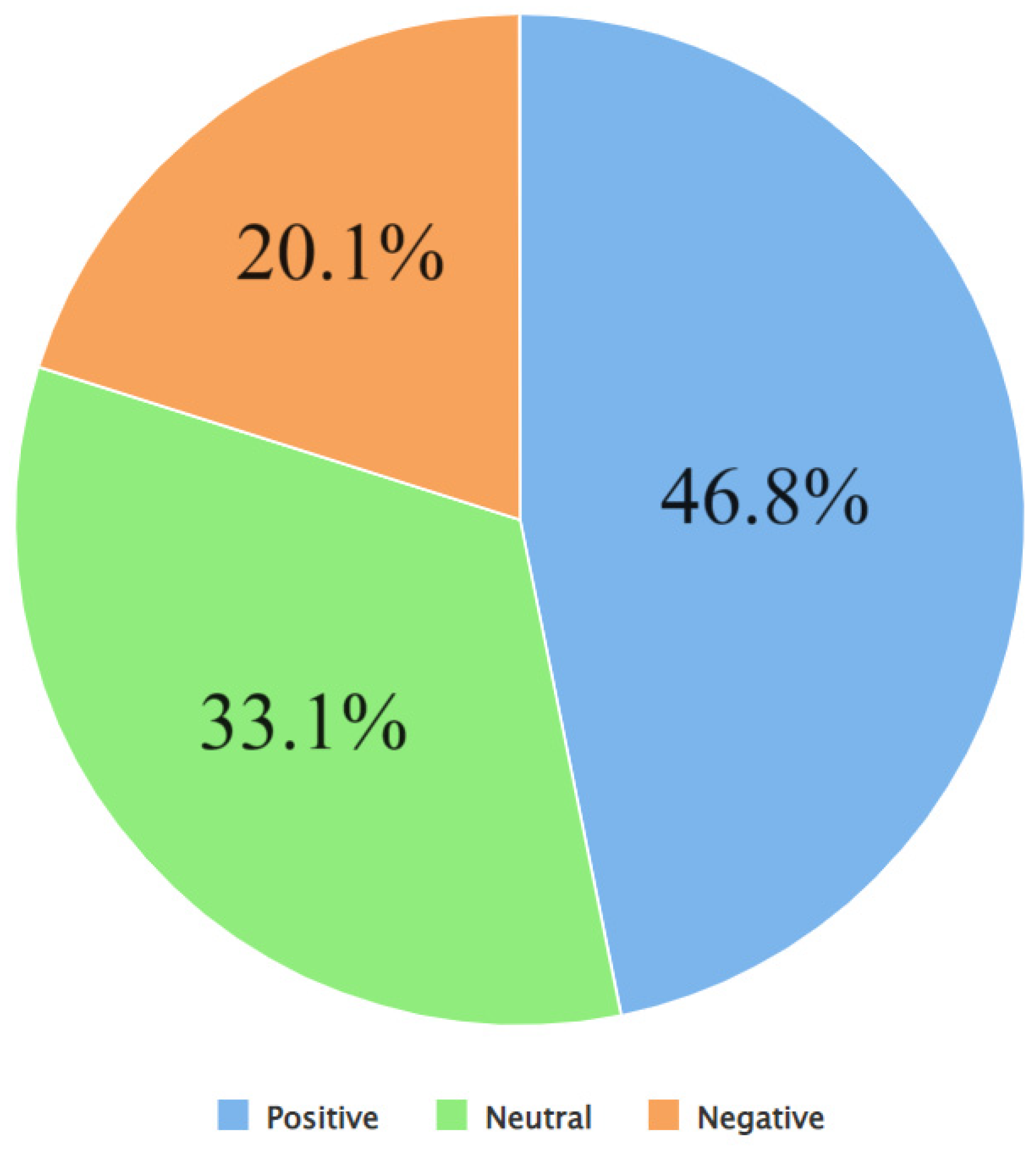
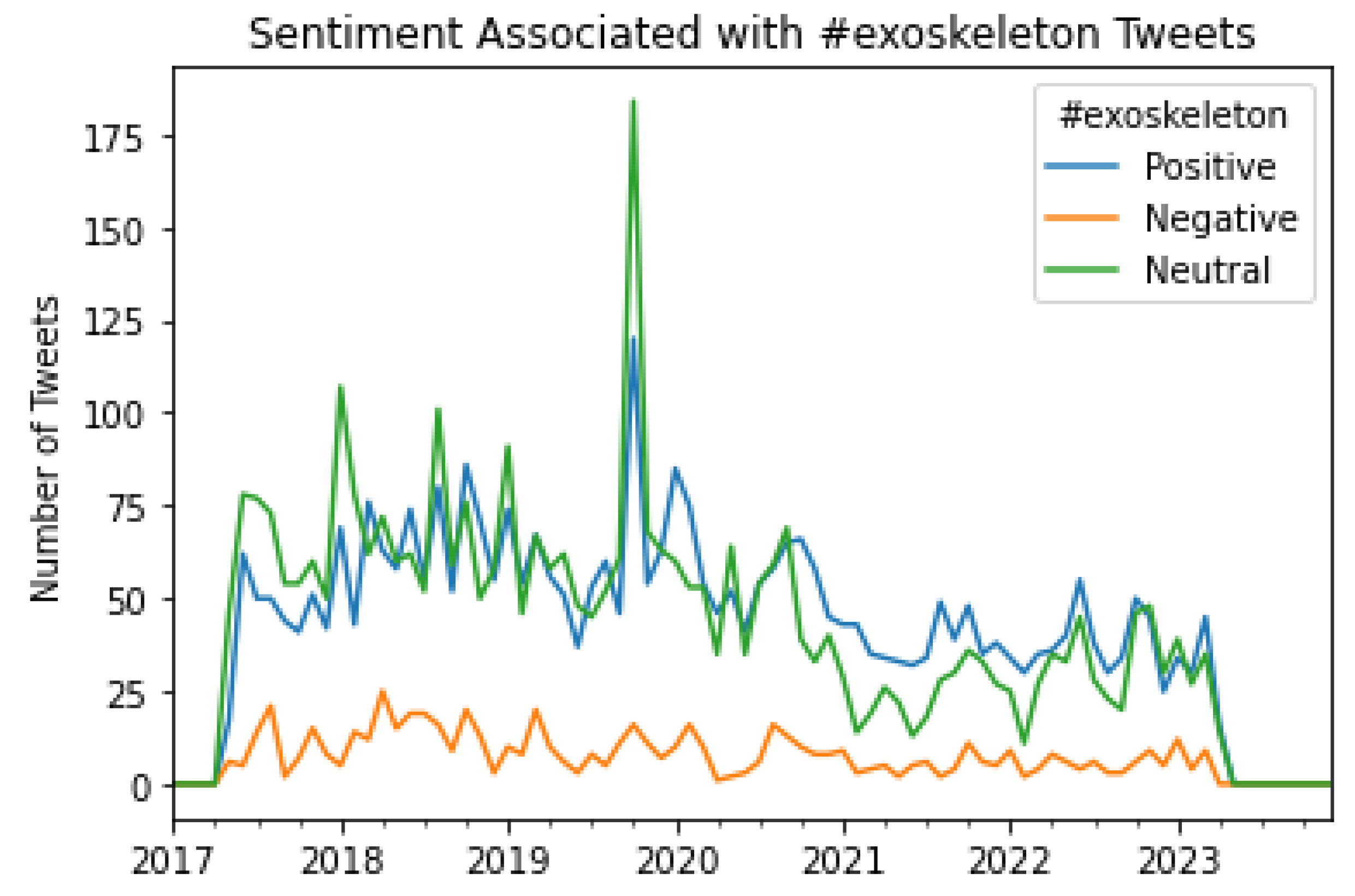
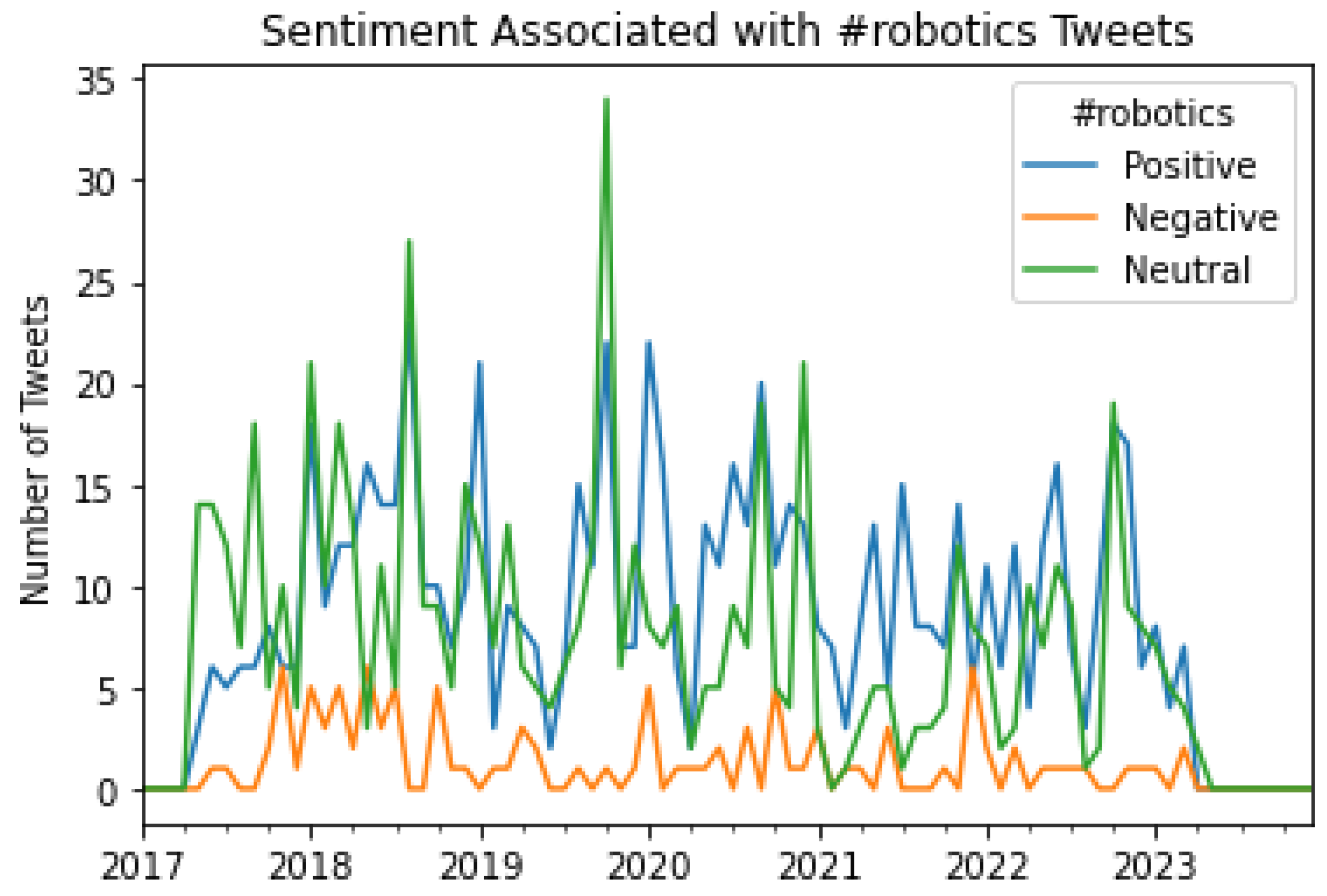
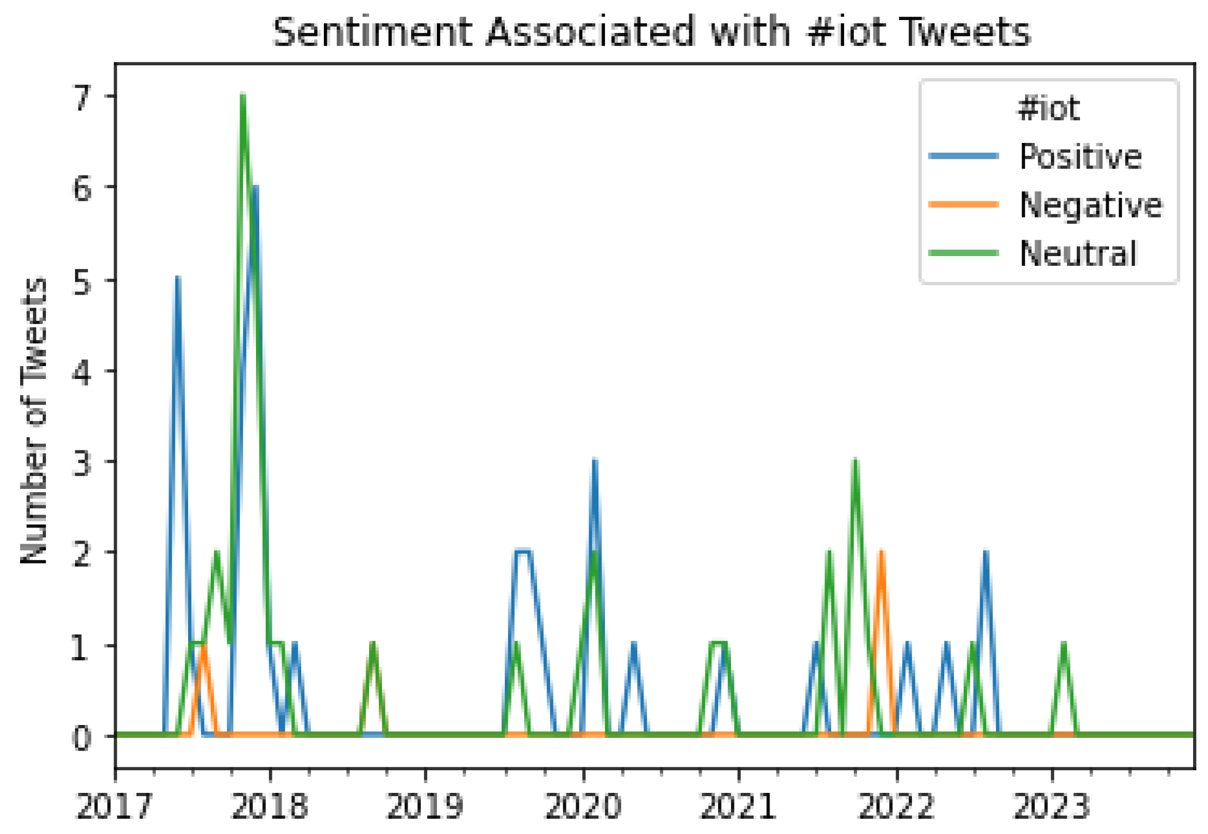
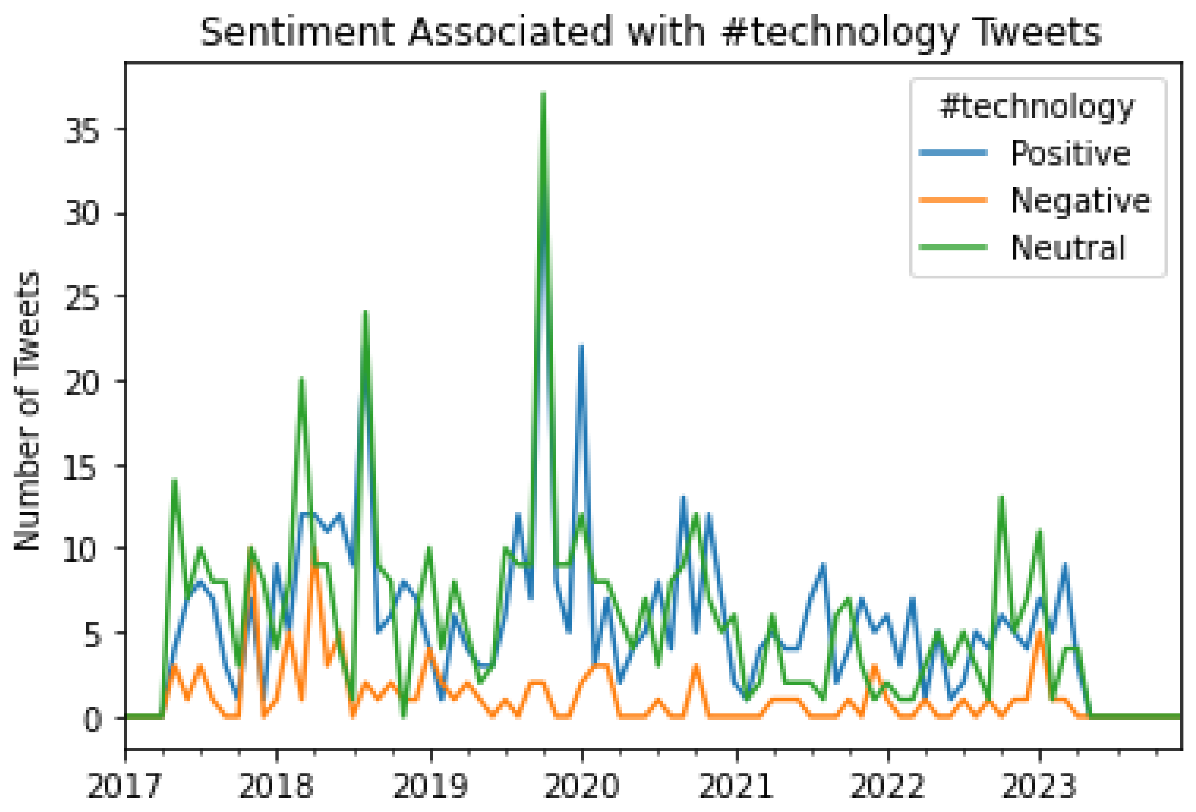
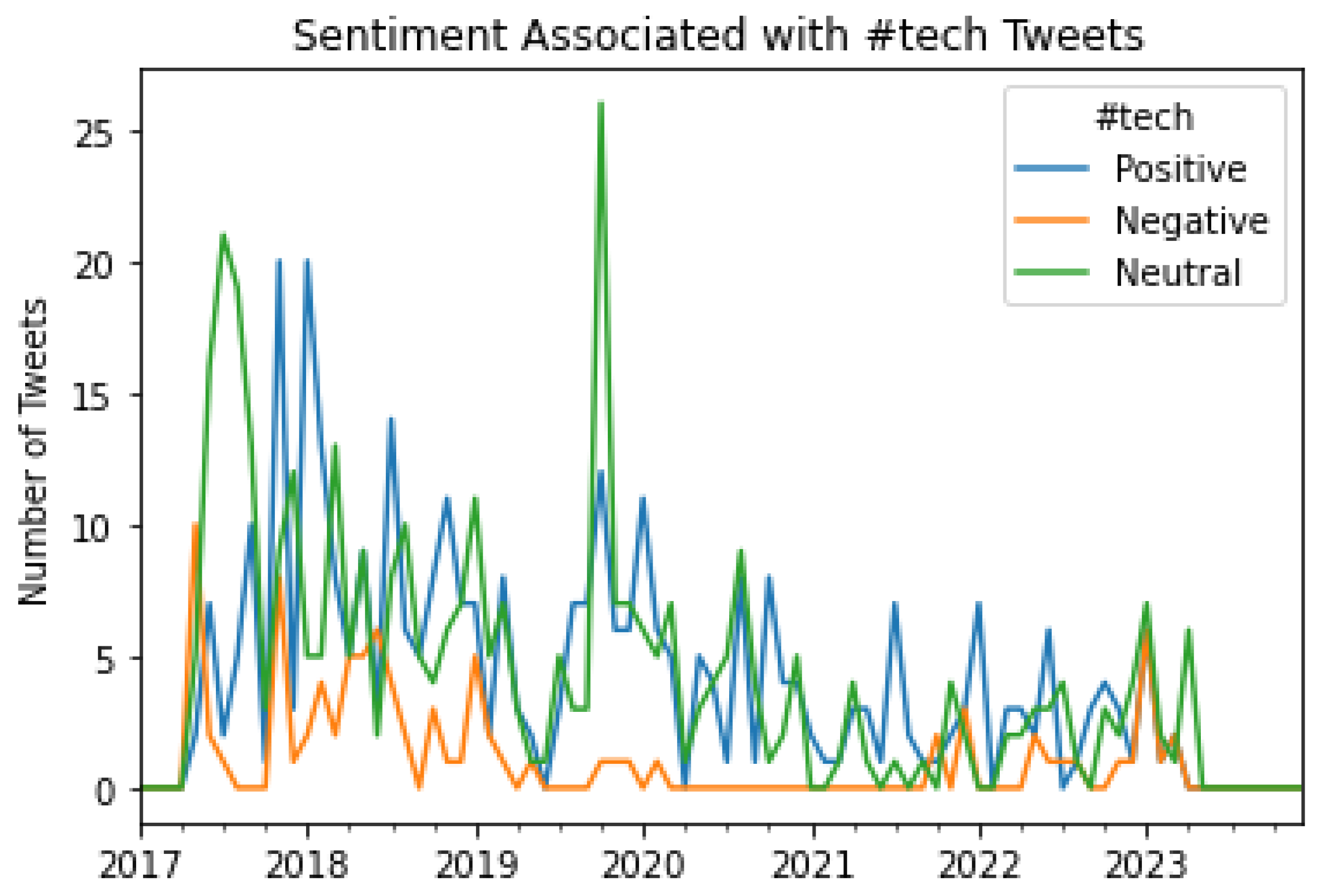
| Work | CA of Tweets about Robots or Robotic Solutions |
CA of Tweets about Wearables (including Wearable Robotics) |
SA of Tweets about Robots or Robotic Solutions |
SA of Tweets about Robots (including Wearable Robotics) |
Fine Grain SA of Tweets about Wearable Robotics |
MLR Model to Predict Tweets about Wearable Robotics |
|---|---|---|---|---|---|---|
| Cramer et al. [18] | √ | |||||
| Salzmann-Erikson et al. [19] | √ | |||||
| Fraser et al. [20] | √ | |||||
| Mubin et al. [21] | √ | |||||
| Barakeh et al. [22] | √ | |||||
| Mahmud et al. [23] | √ | |||||
| Yamanoue et al. [24] | √ | |||||
| Tussyadiah et al. [25] | √ | |||||
| Saxena et al. [26] | √ | |||||
| Adidharma et al. [27] | √ | |||||
| Pillarisetti et al. [28] | √ | |||||
| Keane et al. [29] | √ | |||||
| Sinha et al. [30] | √ | |||||
| El-Gayar et al. [31] | √ | |||||
| Jeong et al. [32] | √ | |||||
| Niininen et al. [33] | √ | |||||
| Thakur et al. [this work] | √ | √ | √ | √ | √ | √ |
5. Conclusions
Author Contributions
Funding
Data Availability Statement
Acknowledgment
Conflicts of Interest
References
- Gundecha, P.; Liu, H. Mining Social Media: A Brief Introduction. In 2012 TutORials in Operations Research; INFORMS, 2012; pp. 1–17.
- Messaoudi, C.; Guessoum, Z.; Ben Romdhane, L. Opinion Mining in Online Social Media: A Survey. Soc. Netw. Anal. Min. 2022, 12. [Google Scholar] [CrossRef]
- Van Looy, A. Definitions, Social Media Types, and Tools. In Social Media Management; Springer International Publishing: Cham, 2022; pp. 21–50. ISBN 9783030990930. [Google Scholar]
- Thakur, N. Social Media Mining and Analysis: A Brief Review of Recent Challenges. Information (Basel) 2023, 14, 484. [Google Scholar] [CrossRef]
- Belle Wong, J.D. Top Social Media Statistics and Trends of 2023. Available online: https://www.forbes.com/advisor/business/social-media-statistics/ (accessed on 23 September 2023).
- Morgan-Lopez, A.A.; Kim, A.E.; Chew, R.F.; Ruddle, P. Predicting Age Groups of Twitter Users Based on Language and Metadata Features. PLoS One 2017, 12, e0183537. [Google Scholar] [CrossRef] [PubMed]
- Martin, M. 29 Twitter Stats That Matter to Marketers in 2023. Available online: https://blog.hootsuite.com/twitter-statistics/ (accessed on 24 September 2023).
- Singh, C. 60+ Twitter Statistics to Skyrocket Your Branding in 2023. Available online: https://www.socialpilot.co/blog/twitter-statistics (accessed on 24 September 2023).
- Taylor, T. 30+ Remarkable Twitter Statistics to Be Aware of in 2023. Available online: https://blog.hubspot.com/marketing/twitter-stats-tips (accessed on 24 September 2023).
- Kemp, S. Twitter Users, Stats, Data, Trends, and More — DataReportal – Global Digital Insights. Available online: https://datareportal.com/essential-twitter-stats (accessed on 24 September 2023).
- Dinesh, S. 8 Facts about Americans and Twitter as It Rebrands to X. Available online: https://www.pewresearch.org/short-reads/2023/07/26/8-facts-about-americans-and-twitter-as-it-rebrands-to-x/ (accessed on 24 September 2023).
- Lin, Y. 10 Twitter Statistics Every Marketer Should Know in 2023 [Infographic]. Available online: https://www.oberlo.com/blog/twitter-statistics (accessed on 24 September 2023).
- Taecharungroj, V. “What Can ChatGPT Do?” Analyzing Early Reactions to the Innovative AI Chatbot on Twitter. Big Data Cogn. Comput. 2023, 7, 35. [Google Scholar] [CrossRef]
- Mujahid, M.; Kanwal, K.; Rustam, F.; Aljadani, W.; Ashraf, I. Arabic ChatGPT Tweets Classification Using RoBERTa and BERT Ensemble Model. ACM Trans. Asian Low-resour. Lang. Inf. Process. 2023, 22, 1–23. [Google Scholar] [CrossRef]
- Tao, W.; Peng, Y. Differentiation and Unity: A Cross-Platform Comparison Analysis of Online Posts’ Semantics of the Russian–Ukrainian War Based on Weibo and Twitter. Commun. Public 2023, 8, 105–124. [Google Scholar] [CrossRef]
- Chen, E.; Ferrara, E. Tweets in Time of Conflict: A Public Dataset Tracking the Twitter Discourse on the War between Ukraine and Russia. Proceedings of the International AAAI Conference on Web and Social Media 2023, 17, 1006–1013. [Google Scholar] [CrossRef]
- Ante, L. How Elon Musk’s Twitter Activity Moves Cryptocurrency Markets. Technol. Forecast. Soc. Change 2023, 186, 122112. [Google Scholar] [CrossRef]
- Kraaijeveld, O.; De Smedt, J. The Predictive Power of Public Twitter Sentiment for Forecasting Cryptocurrency Prices. J. Int. Financ. Mark. Inst. Money 2020, 65, 101188. [Google Scholar] [CrossRef]
- Acharya, S.; Jain, U.; Kumar, R.; Prajapat, S.; Suthar, S.; Ritesh, K. JARVIS: A Virtual Assistant for Smart Communication Available online: https://ijaem.net/issue_dcp/JARVIS%20A%20Virtual%20Assistant%20for%20Smart%20Communication.pdf.
- Cesare, N.; Oladeji, O.; Ferryman, K.; Wijaya, D.; Hendricks-Muñoz, K.D.; Ward, A.; Nsoesie, E.O. Discussions of Miscarriage and Preterm Births on Twitter. Paediatr. Perinat. Epidemiol. 2020, 34, 544–552. [Google Scholar] [CrossRef]
- Kosenko, K.; Winderman, E.; Pugh, A. The Hijacked Hashtag: The Constitutive Features of Abortion Stigma in the #ShoutYourAbortion Twitter Campaign. Int. J. Commun. 2019, 13, 21. [Google Scholar]
- Fox, B. Loneliness and Social Media: A Qualitative Investigation of Young People’s Motivations for Use, and Perceptions of Social Networking Sites. In Emotions and Loneliness in a Networked Society; Springer International Publishing: Cham, 2019; pp. 309–331. ISBN 9783030248819. [Google Scholar]
- Guntuku, S.C.; Schneider, R.; Pelullo, A.; Young, J.; Wong, V.; Ungar, L.; Polsky, D.; Volpp, K.G.; Merchant, R. Studying Expressions of Loneliness in Individuals Using Twitter: An Observational Study. BMJ Open 2019, 9, e030355. [Google Scholar] [CrossRef] [PubMed]
- Allen, J.D.; Hollander, J.; Gualtieri, L.; Alarcon Falconi, T.M.; Savir, S.; Agénor, M. Feasibility of a Twitter Campaign to Promote HPV Vaccine Uptake among Racially/Ethnically Diverse Young Adult Women Living in Public Housing. BMC Public Health 2020, 20. [Google Scholar] [CrossRef]
- Tan, M.J.; Guan, C. Are People Happier in Locations of High Property Value? Spatial Temporal Analytics of Activity Frequency, Public Sentiment and Housing Price Using Twitter Data. Appl. Geogr. 2021, 132, 102474. [Google Scholar] [CrossRef]
- Bovet, A.; Makse, H.A. Influence of Fake News in Twitter during the 2016 US Presidential Election. Nat. Commun. 2019, 10, 1–14. [Google Scholar] [CrossRef] [PubMed]
- Ajao, O.; Bhowmik, D.; Zargari, S. Fake News Identification on Twitter with Hybrid CNN and RNN Models. In Proceedings of the Proceedings of the 9th International Conference on Social Media and Society; ACM: New York, NY, USA, 2018. [Google Scholar]
- Chandra, M.; Reddy, M.; Sehgal, S.; Gupta, S.; Buduru, A.B.; Kumaraguru, P. “A Virus Has No Religion”: Analyzing Islamophobia on Twitter during the COVID-19 Outbreak. In Proceedings of the Proceedings of the 32st ACM Conference on Hypertext and Social Media; ACM: New York, NY, USA, 2021. [Google Scholar]
- Bokányi, E.; Kondor, D.; Dobos, L.; Sebők, T.; Stéger, J.; Csabai, I.; Vattay, G. Race, Religion and the City: Twitter Word Frequency Patterns Reveal Dominant Demographic Dimensions in the United States. Palgrave Commun. 2016, 2, 1–9. [Google Scholar] [CrossRef]
- Amin, S.; Uddin, M.I.; alSaeed, D.H.; Khan, A.; Adnan, M. Early Detection of Seasonal Outbreaks from Twitter Data Using Machine Learning Approaches. Complexity 2021, 2021, 1–12. [Google Scholar] [CrossRef]
- Prieto, V.M.; Matos, S.; Álvarez, M.; Cacheda, F.; Oliveira, J.L. Twitter: A Good Place to Detect Health Conditions. PLoS One 2014, 9, e86191. [Google Scholar] [CrossRef]
- Buccoliero, L.; Bellio, E.; Crestini, G.; Arkoudas, A. Twitter and Politics: Evidence from the US Presidential Elections 2016. J. Mark. Commun. 2020, 26, 88–114. [Google Scholar] [CrossRef]
- Ali, H.; Farman, H.; Yar, H.; Khan, Z.; Habib, S.; Ammar, A. Deep Learning-Based Election Results Prediction Using Twitter Activity. Soft Comput. 2022, 26, 7535–7543. [Google Scholar] [CrossRef]
- Veletsianos, G.; Kimmons, R. Scholars in an Increasingly Open and Digital World: How Do Education Professors and Students Use Twitter? Internet High. Educ. 2016, 30, 1–10. [Google Scholar] [CrossRef]
- Carpenter, J.; Tani, T.; Morrison, S.; Keane, J. Exploring the Landscape of Educator Professional Activity on Twitter: An Analysis of 16 Education-Related Twitter Hashtags. Prof. Dev. Educ. 2022, 48, 784–805. [Google Scholar] [CrossRef]
- Rajabi, S. Grieving the Ambiguous Online: Pregnancy Loss, Meaning Making & Celebrity on Twitter. Fem. Media Stud. 2023, 1–17. [Google Scholar] [CrossRef]
- Moyer, C.A.; Compton, S.D.; Kaselitz, E.; Muzik, M. Pregnancy-Related Anxiety during COVID-19: A Nationwide Survey of 2740 Pregnant Women. Arch. Womens. Ment. Health 2020, 23, 757–765. [Google Scholar] [CrossRef] [PubMed]
- Goetz, S.J.; Heaton, C.; Imran, M.; Pan, Y.; Tian, Z.; Schmidt, C.; Qazi, U.; Ofli, F.; Mitra, P. Food Insufficiency and Twitter Emotions during a Pandemic. Appl. Econ. Perspect. Policy 2023, 45, 1189–1210. [Google Scholar] [CrossRef] [PubMed]
- Ahmad Kontar, N.A.; Mutalib, S.; Muhamed Hanum, H.F.; Abdul-Rahman, S. Exploratory Data Analysis: Food Security Risk among Twitter Users. J. Comput. Sci. Comput. Math. 2023, 13, 15–19. [Google Scholar] [CrossRef]
- Knudsen, B.; Høeg, T.B.; Prasad, V. Analysis of Tweets Discussing the Risk of Mpox among Children and Young People in School (May-Oct 2022): Public Health Experts on Twitter Consistently Exaggerated Risks and Infrequently Reported Accurate Information. bioRxiv 2023.
- Edinger, A.; Valdez, D.; Walsh-Buhi, E.; Trueblood, J.S.; Lorenzo-Luaces, L.; Rutter, L.A.; Bollen, J. Misinformation and Public Health Messaging in the Early Stages of the Mpox Outbreak: Mapping the Twitter Narrative with Deep Learning. J. Med. Internet Res. 2023, 25, e43841. [Google Scholar] [CrossRef]
- Wakamiya, S.; Kawai, Y.; Aramaki, E. Twitter-Based Influenza Detection after Flu Peak via Tweets with Indirect Information: Text Mining Study. JMIR Public Health Surveill. 2018, 4, e65. [Google Scholar] [CrossRef]
- Lee, K.; Agrawal, A.; Choudhary, A. Real-Time Disease Surveillance Using Twitter Data: Demonstration on Flu and Cancer. In Proceedings of the Proceedings of the 19th ACM SIGKDD international conference on Knowledge discovery and data mining; ACM: New York, NY, USA, 2013. [Google Scholar]
- Jain, V.K.; Kumar, S. An Effective Approach to Track Levels of Influenza-A (H1N1) Pandemic in India Using Twitter. Procedia Comput. Sci. 2015, 70, 801–807. [Google Scholar] [CrossRef]
- Ahmed, W.; Bath, P.A.; Sbaffi, L.; Demartini, G. Novel Insights into Views towards H1N1 during the 2009 Pandemic: A Thematic Analysis of Twitter Data. Health Info. Libr. J. 2019, 36, 60–72. [Google Scholar] [CrossRef] [PubMed]
- Ng, R.; Indran, N.; Liu, L. Ageism on Twitter during the COVID-19 Pandemic. J. Soc. Issues 2022, 78, 842–859. [Google Scholar] [CrossRef]
- Hua, Y.; Jiang, H.; Lin, S.; Yang, J.; Plasek, J.M.; Bates, D.W.; Zhou, L. Using Twitter Data to Understand Public Perceptions of Approved versus Off-Label Use for COVID-19-Related Medications. J. Am. Med. Inform. Assoc. 2022, 29, 1668–1678. [Google Scholar] [CrossRef] [PubMed]
- Olar, M.-L.; Leba, M.; Risteiu, M. Exoskeleton - Wearable Devices. Literature Review. MATEC Web Conf. 2021, 342, 05005. [Google Scholar] [CrossRef]
- Yang, C.-J.; Zhang, J.-F.; Chen, Y.; Dong, Y.-M.; Zhang, Y. A Review of Exoskeleton-Type Systems and Their Key Technologies. Proc Inst Mech Eng Part C 2008, 222, 1599–1612. [Google Scholar] [CrossRef]
- Palazzi, E.; Luzi, L.; Dimo, E.; Meneghetti, M.; Vicario, R.; Luzia, R.F.; Vertechy, R.; Calanca, A. An Affordable Upper-Limb Exoskeleton Concept for Rehabilitation Applications. Technologies (Basel) 2022, 10, 22. [Google Scholar] [CrossRef]
- Laubscher, C.A.; Goo, A.; Farris, R.J.; Sawicki, J.T. Hybrid Impedance-Sliding Mode Switching Control of the Indego Explorer Lower-Limb Exoskeleton in Able-Bodied Walking. J. Intell. Robot. Syst. 2022, 104. [Google Scholar] [CrossRef]
- Zoss, A.B.; Kazerooni, H.; Chu, A. Biomechanical Design of the Berkeley Lower Extremity Exoskeleton (BLEEX). IEEE ASME Trans. Mechatron. 2006, 11, 128–138. [Google Scholar] [CrossRef]
- Høyer, E.; Opheim, A.; Jørgensen, V. Implementing the Exoskeleton Ekso GTTM for Gait Rehabilitation in a Stroke Unit – Feasibility, Functional Benefits and Patient Experiences. Disabil. Rehabil. Assist. Technol. 2022, 17, 473–479. [Google Scholar] [CrossRef]
- van Kammen, K.; Boonstra, A.M.; van der Woude, L.H.V.; Reinders-Messelink, H.A.; den Otter, R. The Combined Effects of Guidance Force, Bodyweight Support and Gait Speed on Muscle Activity during Able-Bodied Walking in the Lokomat. Clin. Biomech. (Bristol, Avon) 2016, 36, 65–73. [Google Scholar] [CrossRef]
- Gull, M.A.; Bai, S.; Bak, T. A Review on Design of Upper Limb Exoskeletons. Robotics 2020, 9, 16. [Google Scholar] [CrossRef]
- Comani, S.; Velluto, L.; Schinaia, L.; Cerroni, G.; Serio, A.; Buzzelli, S.; Sorbi, S.; Guarnieri, B. Monitoring Neuro-Motor Recovery from Stroke with High-Resolution EEG, Robotics and Virtual Reality: A Proof of Concept. IEEE Trans. Neural Syst. Rehabil. Eng. 2015, 23, 1106–1116. [Google Scholar] [CrossRef]
- Grimm, F.; Walter, A.; Spüler, M.; Naros, G.; Rosenstiel, W.; Gharabaghi, A. Hybrid Neuroprosthesis for the Upper Limb: Combining Brain-Controlled Neuromuscular Stimulation with a Multi-Joint Arm Exoskeleton. Front. Neurosci. 2016, 10. [Google Scholar] [CrossRef] [PubMed]
- Sarkisian, S.V.; Ishmael, M.K.; Lenzi, T. Self-Aligning Mechanism Improves Comfort and Performance with a Powered Knee Exoskeleton. IEEE Trans. Neural Syst. Rehabil. Eng. 2021, 29, 629–640. [Google Scholar] [CrossRef]
- van der Have, A.; Rossini, M.; Rodriguez-Guerrero, C.; Van Rossom, S.; Jonkers, I. The Exo4Work Shoulder Exoskeleton Effectively Reduces Muscle and Joint Loading during Simulated Occupational Tasks above Shoulder Height. Appl. Ergon. 2022, 103, 103800. [Google Scholar] [CrossRef] [PubMed]
- Zahedi, A.; Wang, Y.; Martinez-Hernandez, U.; Zhang, D. A Wearable Elbow Exoskeleton for Tremor Suppression Equipped with Rotational Semi-Active Actuator. Mech. Syst. Signal Process. 2021, 157, 107674. [Google Scholar] [CrossRef]
- Peng, X.; Acosta-Sojo, Y.; Wu, M.I.; Stirling, L. Actuation Timing Perception of a Powered Ankle Exoskeleton and Its Associated Ankle Angle Changes during Walking. IEEE Trans. Neural Syst. Rehabil. Eng. 2022, 30, 869–877. [Google Scholar] [CrossRef]
- Liu, H.; Zeng, B.; Liu, X.; Zhu, X.; Song, H. Detection of Human Lifting State Based on Long Short-Term Memory for Wearable Waist Exoskeleton. In Lecture Notes in Electrical Engineering; Springer Singapore: Singapore, 2022; pp. 301–310. ISBN 9789811663277. [Google Scholar]
- Ishmael, M.K.; Archangeli, D.; Lenzi, T. A Powered Hip Exoskeleton with High Torque Density for Walking, Running, and Stair Ascent. IEEE ASME Trans. Mechatron. 2022, 27, 4561–4572. [Google Scholar] [CrossRef]
- Garosi, E.; Mazloumi, A.; Jafari, A.H.; Keihani, A.; Shamsipour, M.; Kordi, R.; Kazemi, Z. Design and Ergonomic Assessment of a Passive Head/Neck Supporting Exoskeleton for Overhead Work Use. Appl. Ergon. 2022, 101, 103699. [Google Scholar] [CrossRef]
- Song, J.; Zhu, A.; Tu, Y.; Zou, J. Multijoint Passive Elastic Spine Exoskeleton for Stoop Lifting Assistance. Int. J. Adv. Robot. Syst. 2021, 18, 172988142110620. [Google Scholar] [CrossRef]
- Dragusanu, M.; Iqbal, M.Z.; Baldi, T.L.; Prattichizzo, D.; Malvezzi, M. Design, Development, and Control of a Hand/Wrist Exoskeleton for Rehabilitation and Training. IEEE Trans. Robot. 2022, 38, 1472–1488. [Google Scholar] [CrossRef]
- Li, G.; Cheng, L.; Sun, N. Design, Manipulability Analysis and Optimization of an Index Finger Exoskeleton for Stroke Rehabilitation. Mech. Mach. Theory 2022, 167, 104526. [Google Scholar] [CrossRef]
- Bär, M.; Steinhilber, B.; Rieger, M.A.; Luger, T. The Influence of Using Exoskeletons during Occupational Tasks on Acute Physical Stress and Strain Compared to No Exoskeleton – A Systematic Review and Meta-Analysis. Appl. Ergon. 2021, 94, 103385. [Google Scholar] [CrossRef]
- Sawicki, G.S.; Beck, O.N.; Kang, I.; Young, A.J. The Exoskeleton Expansion: Improving Walking and Running Economy. J. Neuroeng. Rehabil. 2020, 17. [Google Scholar] [CrossRef] [PubMed]
- Massardi, S.; Rodriguez-Cianca, D.; Pinto-Fernandez, D.; Moreno, J.C.; Lancini, M.; Torricelli, D. Characterization and Evaluation of Human–Exoskeleton Interaction Dynamics: A Review. Sensors (Basel) 2022, 22, 3993. [Google Scholar] [CrossRef] [PubMed]
- Exoskeleton Market Size, Share & Trends Analysis Report, by Mobility, by Technology, by Extremity, by End-Use, by Region, and Segment Forecasts, 2023 - 2030. Available online: https://www.grandviewresearch.com/industry-analysis/exoskeleton-market (accessed on 24 September 2023).
- Bogue, R. Exoskeletons: A Review of Recent Progress. Ind. Rob. 2022, 49, 813–818. [Google Scholar] [CrossRef]
- Cardona, M.; Solanki, V.K.; García Cena, C.E. Exoskeleton Robots for Rehabilitation and Healthcare Devices; Springer Singapore: Singapore, 2020; ISBN 9789811547317. [Google Scholar]
- Tan, K.; Koyama, S.; Sakurai, H.; Teranishi, T.; Kanada, Y.; Tanabe, S. Wearable Robotic Exoskeleton for Gait Reconstruction in Patients with Spinal Cord Injury: A Literature Review. J. Orthop. Translat. 2021, 28, 55–64. [Google Scholar] [CrossRef]
- Kandilakis, C.; Sasso-Lance, E. Exoskeletons for Personal Use after Spinal Cord Injury. Arch. Phys. Med. Rehabil. 2021, 102, 331–337. [Google Scholar] [CrossRef] [PubMed]
- Jung, M.M.; Ludden, G.D.S. What Do Older Adults and Clinicians Think about Traditional Mobility Aids and Exoskeleton Technology? ACM Trans. Hum. Robot Interact. 2019, 8, 1–17. [Google Scholar] [CrossRef]
- Bunge, L.R.; Davidson, A.J.; Helmore, B.R.; Mavrandonis, A.D.; Page, T.D.; Schuster-Bayly, T.R.; Kumar, S. Effectiveness of Powered Exoskeleton Use on Gait in Individuals with Cerebral Palsy: A Systematic Review. PLoS One 2021, 16, e0252193. [Google Scholar] [CrossRef]
- Kamiński, M.; Muth, A.; Bogdański, P. Smoking, Vaping, and Tobacco Industry during COVID-19 Pandemic: Twitter Data Analysis. Cyberpsychol. Behav. Soc. Netw. 2020, 23, 811–817. [Google Scholar] [CrossRef]
- Souza, T.T.P.; Kolchyna, O.; Treleaven, P.C.; Aste, T. Twitter Sentiment Analysis Applied to Finance: A Case Study in the Retail Industry. arXiv [cs.CY] 2015. [Google Scholar]
- Pons, A.; Rius, J.; Vintró, C.; Gallart, A. Analysis of Twitter Posts for Evaluation of Corporate Social Responsibility in the Leather Industry. J. Eng. Fiber. Fabr. 2022, 17, 155892502211318. [Google Scholar] [CrossRef]
- Leung, X.Y.; Bai, B.; Stahura, K.A. The Marketing Effectiveness of Social Media in the Hotel Industry: A Comparison of Facebook and Twitter. J. Hosp. Tour. Res. 2015, 39, 147–169. [Google Scholar] [CrossRef]
- Misopoulos, F.; Mitic, M.; Kapoulas, A.; Karapiperis, C. Uncovering Customer Service Experiences with Twitter: The Case of Airline Industry. Manag. Decis. 2014, 52, 705–723. [Google Scholar] [CrossRef]
- Shukri, S.E.; Yaghi, R.I.; Aljarah, I.; Alsawalqah, H. Twitter Sentiment Analysis: A Case Study in the Automotive Industry. In Proceedings of the 2015 IEEE Jordan Conference on Applied Electrical Engineering and Computing Technologies (AEECT); IEEE, 2015. [CrossRef]
- Criswell, J.; Canty, N. Deconstructing Social Media: An Analysis of Twitter and Facebook Use in the Publishing Industry. Publ. Res. Q. 2014, 30, 352–376. [Google Scholar] [CrossRef]
- Parganas, P.; Anagnostopoulos, C.; Chadwick, S. ‘You’Ll Never Tweet Alone’: Managing Sports Brands through Social Media. J. Brand Manag. 2015, 22, 551–568. [Google Scholar] [CrossRef]
- Paredes-Corvalan, D.; Pezoa-Fuentes, C.; Silva-Rojas, G.; Valenzuela Rojas, I.; Castillo-Vergara, M. Engagement of the E-Commerce Industry in the US, According to Twitter in the Period of the COVID-19 Pandemic. Heliyon 2023, 9, e16881. [Google Scholar] [CrossRef]
- Garcia-Rivera, D.; Matamoros-Rojas, S.; Pezoa-Fuentes, C.; Veas-González, I.; Vidal-Silva, C. Engagement on Twitter, a Closer Look from the Consumer Electronics Industry. J. Theor. Appl. Electron. Commer. Res. 2022, 17, 558–570. [Google Scholar] [CrossRef]
- Wonneberger, A.; Hellsten, I.R.; Jacobs, S.H.J. Hashtag Activism and the Configuration of Counterpublics: Dutch Animal Welfare Debates on Twitter. Inf. Commun. Soc. 2021, 24, 1694–1711. [Google Scholar] [CrossRef]
- Aleti, T.; Harrigan, P.; Cheong, M.; Turner, W. An Investigation of How the Australian Brewing Industry Influence Consumers on Twitter. Aust. J. Inf. Syst. 2016, 20. [Google Scholar] [CrossRef]
- Komorowski, M.; Huu, T.D.; Deligiannis, N. Twitter Data Analysis for Studying Communities of Practice in the Media Industry. Telemat. Inform. 2018, 35, 195–212. [Google Scholar] [CrossRef]
- Ghanadpour, S.H.; Shokouhyar, S.; Pourabbasi, M. Effective End of life (EOL) Products Management in Mobile Phone Industry with Using Twitter Data Analysis Perspective. Environ. Dev. Sustain. 2023, 25, 11337–11366. [Google Scholar] [CrossRef]
- Durand-Moreau, Q.; Mackenzie, G.; Adisesh, A.; Straube, S.; Chan, X.H.S.; Zelyas, N.; Greenhalgh, T. Twitter Analytics to Inform Provisional Guidance for COVID-19 Challenges in the Meatpacking Industry. Ann. Work Expo. Health 2021, 65, 373–376. [Google Scholar] [CrossRef]
- Casadei, P.; Lee, N. Global Cities, Creative Industries and Their Representation on Social Media: A Micro-Data Analysis of Twitter Data on the Fashion Industry. Environ. Plan. A 2020, 52, 1195–1220. [Google Scholar] [CrossRef]
- Sama, T.B.; Konttinen, I.; Hiilamo, H. Alcohol Industry Arguments for Liberalizing Alcohol Policy in Finland: Analysis of Twitter Data. J. Stud. Alcohol Drugs 2021, 82, 279–287. [Google Scholar] [CrossRef]
- Cramer, H.; Büttner, S. Things That Tweet, Check-in and Are Befriended: Two Explorations on Robotics & Social Media. In Proceedings of the Proceedings of the 6th international conference on Human-robot interaction; ACM: New York, NY, USA, 2011. [Google Scholar]
- Salzmann-Erikson, M.; Eriksson, H. Absorbability, Applicability and Availability in Nursing and Care Robots: A Thematic Analysis of Twitter Postings. Telemat. Inform. 2018, 35, 1553–1560. [Google Scholar] [CrossRef]
- Fraser, K.C.; Zeller, F.; Smith, D.H.; Mohammad, S.; Rudzicz, F. How Do We Feel When a Robot Dies? Emotions Expressed on Twitter before and after Hitch. In Proceedings of the Proceedings of the Tenth Workshop on Computational Approaches to Subjectivity, Sentiment and Social Media Analysis; Association for Computational Linguistics: Stroudsburg, PA, USA, 2019; pp. 62–71.
- Mubin, O.; Khan, A.; Obaid, M. #naorobot: Exploring Nao Discourse on Twitter. In Proceedings of the Proceedings of the 28th Australian Conference on Computer-Human Interaction - OzCHI ’16; ACM Press: New York, New York, USA, 2016. [Google Scholar]
- Barakeh, Z.A.; Alkork, S.; Karar, A.S.; Said, S.; Beyrouthy, T. Pepper Humanoid Robot as a Service Robot: A Customer Approach. In Proceedings of the 2019 3rd International Conference on Bio-engineering for Smart Technologies (BioSMART); IEEE, 2019. [CrossRef]
- Mahmud, J.; Fei, G.; Xu, A.; Pal, A.; Zhou, M. Predicting Attitude and Actions of Twitter Users. In Proceedings of the Proceedings of the 21st International Conference on Intelligent User Interfaces; ACM: New York, NY, USA, 2016. [Google Scholar]
- Yamanoue, T.; Yoshimura, K.; Oda, K.; Shimozono, K. A Wearable LED Matrix Sign System Which Shows a Tweet of Twitter and Its Application to Campus Guiding and Emergency Evacuation. In Proceedings of the Proceedings of the 2015 ACM SIGUCCS Annual Conference; ACM: New York, NY, USA, 2015.
- Tussyadiah, I. Expectation of Travel Experiences with Wearable Computing Devices. In Information and Communication Technologies in Tourism 2014; Springer International Publishing: Cham, 2013; pp. 539–552. ISBN 9783319039725. [Google Scholar]
- Saxena, R.C.; Lehmann, A.E.; Hight, A.E.; Darrow, K.; Remenschneider, A.; Kozin, E.D.; Lee, D.J. Social Media Utilization in the Cochlear Implant Community. J. Am. Acad. Audiol. 2015, 26, 197–204. [Google Scholar] [CrossRef]
- Adidharma, W.; Latack, K.R.; Colohan, S.M.; Morrison, S.D.; Cederna, P.S. Breast Implant Illness: Are Social Media and the Internet Worrying Patients Sick? Plast. Reconstr. Surg. 2020, 145, 225e–227e. [Google Scholar] [CrossRef]
- Pillarisetti, L.; Kerr, B.R.; Moreno, M. Exploring the Discussion of Nexplanon (Etonogestrel Birth Control Implant) on Twitter. Available online: https://digitalhealth.med.brown.edu/sites/default/files/Lekha%20P.pdf (accessed on 24 September 2023).
- Keane, G.; Chi, D.; Ha, A.Y.; Myckatyn, T.M. En Bloc Capsulectomy for Breast Implant Illness: A Social Media Phenomenon? Aesthet. Surg. J. 2021, 41, 448–459. [Google Scholar] [CrossRef]
- Sinha, N.; Singh, P.; Gupta, M.; Singh, P. Robotics at Workplace: An Integrated Twitter Analytics – SEM Based Approach for Behavioral Intention to Accept. Int. J. Inf. Manage. 2020, 55, 102210. [Google Scholar] [CrossRef]
- El-Gayar, O.; Nasralah, T.; Elnoshokaty, A. Wearable Devices for Health and Wellbeing: Design Insights from Twitter. In Proceedings of the Hawaii International Conference on System Sciences 2019 (HICSS-52); 2019.
- Jeong, W.-K.; Shin, D.-H. Analyzing Smart Watch Recognition and Response in Korea Using Text Mining Analysis Focusing on Twitter. J. Digit. Contents Soc. 2023, 24, 195–204. [Google Scholar] [CrossRef]
- Niininen, O.; Singaraju, S.; Arango, L. The Human RFID Implants Introduce a New Level of Human-Computer Interaction: Twitter Topic Detection Gauges Consumer Opinions; EasyChair, 2023. [Google Scholar]
- Thakur, N. Twitter Big Data as a Resource for Exoskeleton Research: A Large-Scale Dataset of about 140,000 Tweets from 2017–2022 and 100 Research Questions. Analytics 2022, 1, 72–97. [Google Scholar] [CrossRef]
- Mierswa, I.; Wurst, M.; Klinkenberg, R.; Scholz, M.; Euler, T. YALE: Rapid Prototyping for Complex Data Mining Tasks. In Proceedings of the Proceedings of the 12th ACM SIGKDD international conference on Knowledge discovery and data mining; ACM: New York, NY, USA, 2006. [Google Scholar]
- Twitter Advanced Search. Available online: https://twitter.com/search-advanced?lang=en (accessed on 24 September 2023).
- Wilkinson, M.D.; Dumontier, M.; Aalbersberg, I.J.; Appleton, G.; Axton, M.; Baak, A.; Blomberg, N.; Boiten, J.-W.; da Silva Santos, L.B.; Bourne, P.E.; et al. The FAIR Guiding Principles for Scientific Data Management and Stewardship. Sci. Data 2016, 3, 1–9. [Google Scholar] [CrossRef] [PubMed]
- Xue, J.; Chen, J.; Chen, C.; Zheng, C.; Li, S.; Zhu, T. Public Discourse and Sentiment during the COVID 19 Pandemic: Using Latent Dirichlet Allocation for Topic Modeling on Twitter. PLoS One 2020, 15, e0239441. [Google Scholar] [CrossRef] [PubMed]
- Rezapour, R.; Wang, L.; Abdar, O.; Diesner, J. Identifying the Overlap between Election Result and Candidates’ Ranking Based on Hashtag-Enhanced, Lexicon-Based Sentiment Analysis. In Proceedings of the 2017 IEEE 11th International Conference on Semantic Computing (ICSC); IEEE, 2017. [CrossRef]
- Qaseem, D.M.; Ali, N.; Akram, W.; Ullah, A.; Polat, K. Movie Success-Rate Prediction System through Optimal Sentiment Analysis Available online: https://iecscience.org/public/uploads/jpapers/202210/63jv6Sz1Y6sdsUtnflF9dmTy3XyB2JHLZ2IGClPo.pdf.
- Hutto, C.; Gilbert, E. VADER: A Parsimonious Rule-Based Model for Sentiment Analysis of Social Media Text. Proceedings of the International AAAI Conference on Web and Social Media 2014, 8, 216–225. [Google Scholar] [CrossRef]
- González-Ibáñez, R.; Muresan, S.; Wacholder, N. Identifying Sarcasm in Twitter: A Closer Look. Available online: https://aclanthology.org/P11-2102.pdf (accessed on 24 September 2023).
- Reyes, A.; Rosso, P.; Buscaldi, D. From Humor Recognition to Irony Detection: The Figurative Language of Social Media. Data Knowl. Eng. 2012, 74, 1–12. [Google Scholar] [CrossRef]
- Moores, B.; Mago, V. A Survey on Automated Sarcasm Detection on Twitter. arXiv [cs.CL] 2022. [Google Scholar]
- Kunneman, F.; Liebrecht, C.; van Mulken, M.; van den Bosch, A. Signaling Sarcasm: From Hyperbole to Hashtag. Inf. Process. Manag. 2015, 51, 500–509. [Google Scholar] [CrossRef]
- Kreuz, R.J.; Caucci, G.M. Lexical Influences on the Perception of Sarcasm. Available online: https://aclanthology.org/W07-0101.pdf (accessed on 24 September 2023).
- Phuvipadawat, S.; Murata, T. Breaking News Detection and Tracking in Twitter. In Proceedings of the 2010 IEEE/WIC/ACM International Conference on Web Intelligence and Intelligent Agent Technology; IEEE, 2010. [CrossRef]
- Bruns, A.; Burgess, J. RESEARCHING NEWS DISCUSSION ON TWITTER: New Methodologies. Journal. Stud. 2012, 13, 801–814. [Google Scholar] [CrossRef]
- Roberge, J.-M. Using Data from Online Social Networks in Conservation Science: Which Species Engage People the Most on Twitter? Biodivers. Conserv. 2014, 23, 715–726. [Google Scholar] [CrossRef]
- J-Hartmann/Emotion-English-Distilroberta-Base · Hugging Face. Available online: https://huggingface.co/j-hartmann/emotion-english-distilroberta-base? (accessed on 25 September 2023).
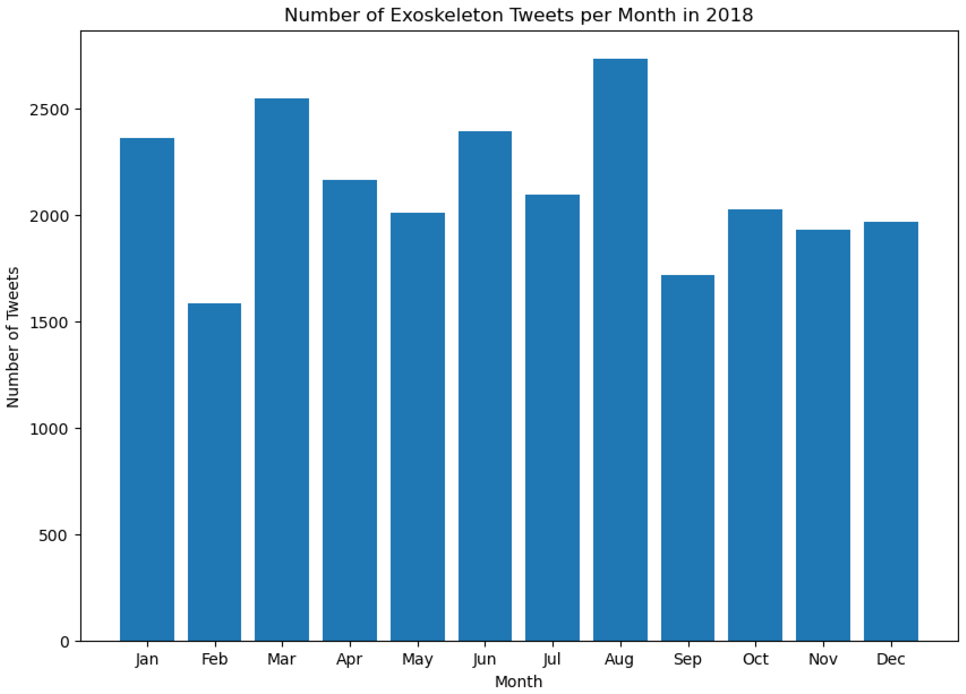
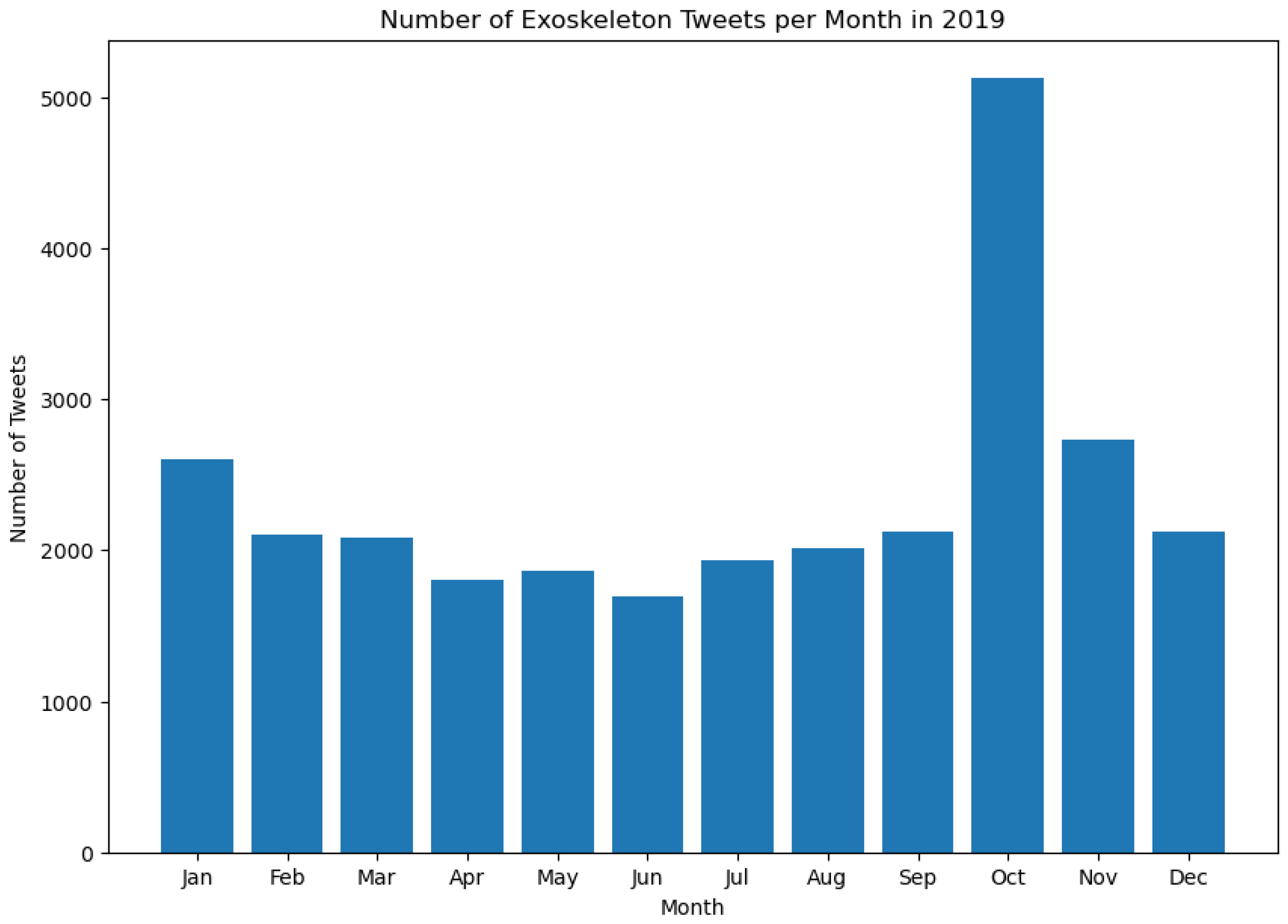
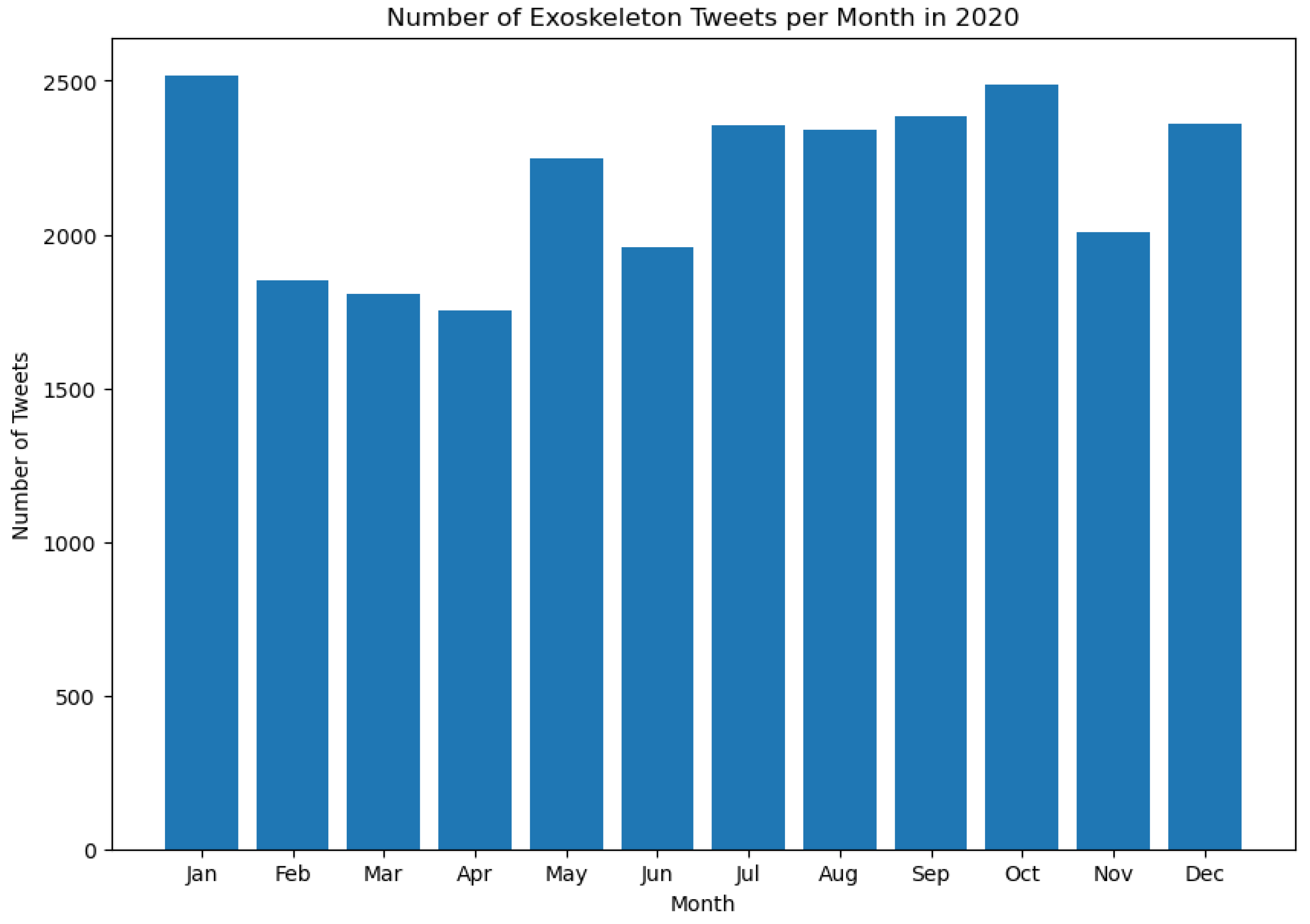
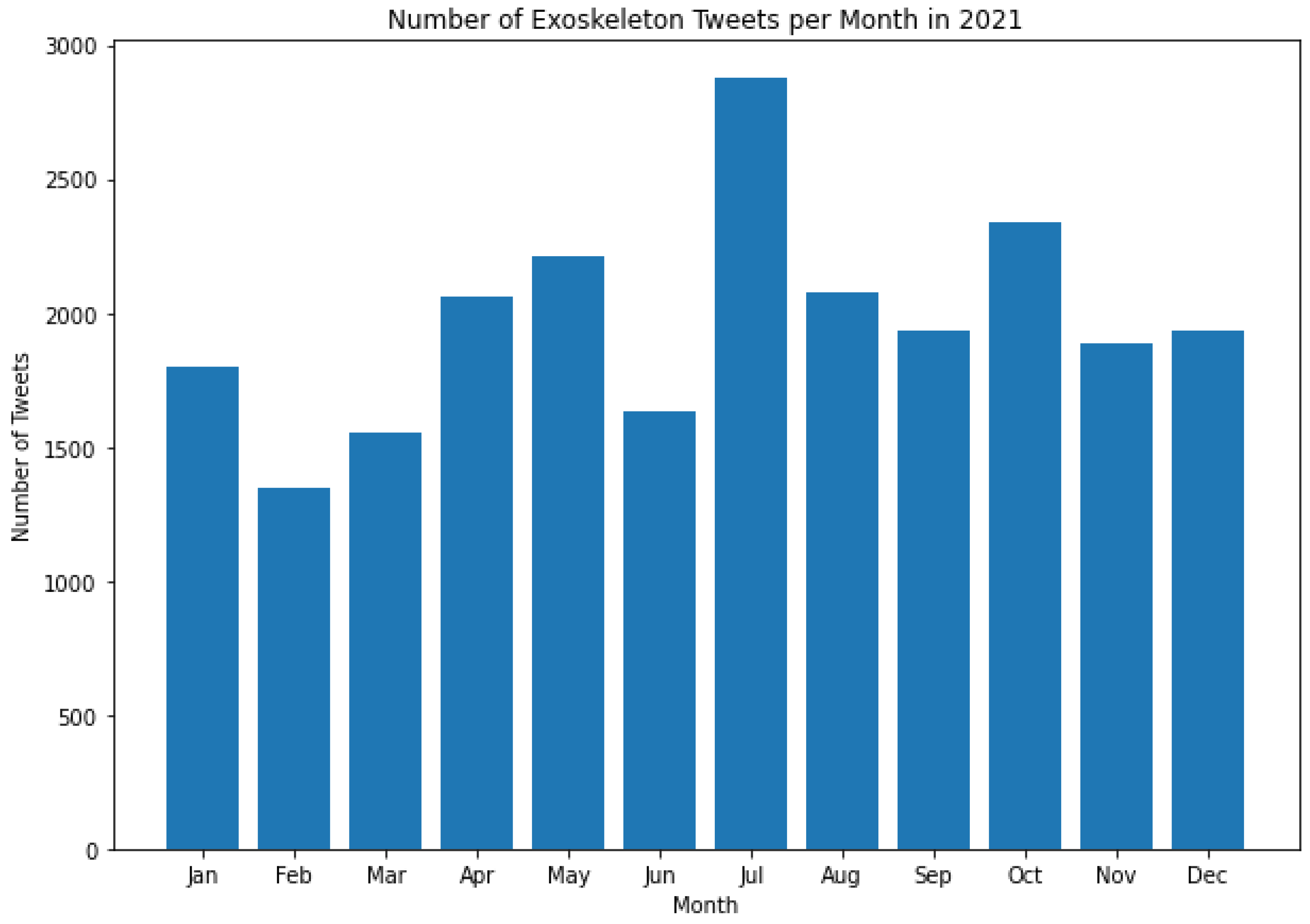
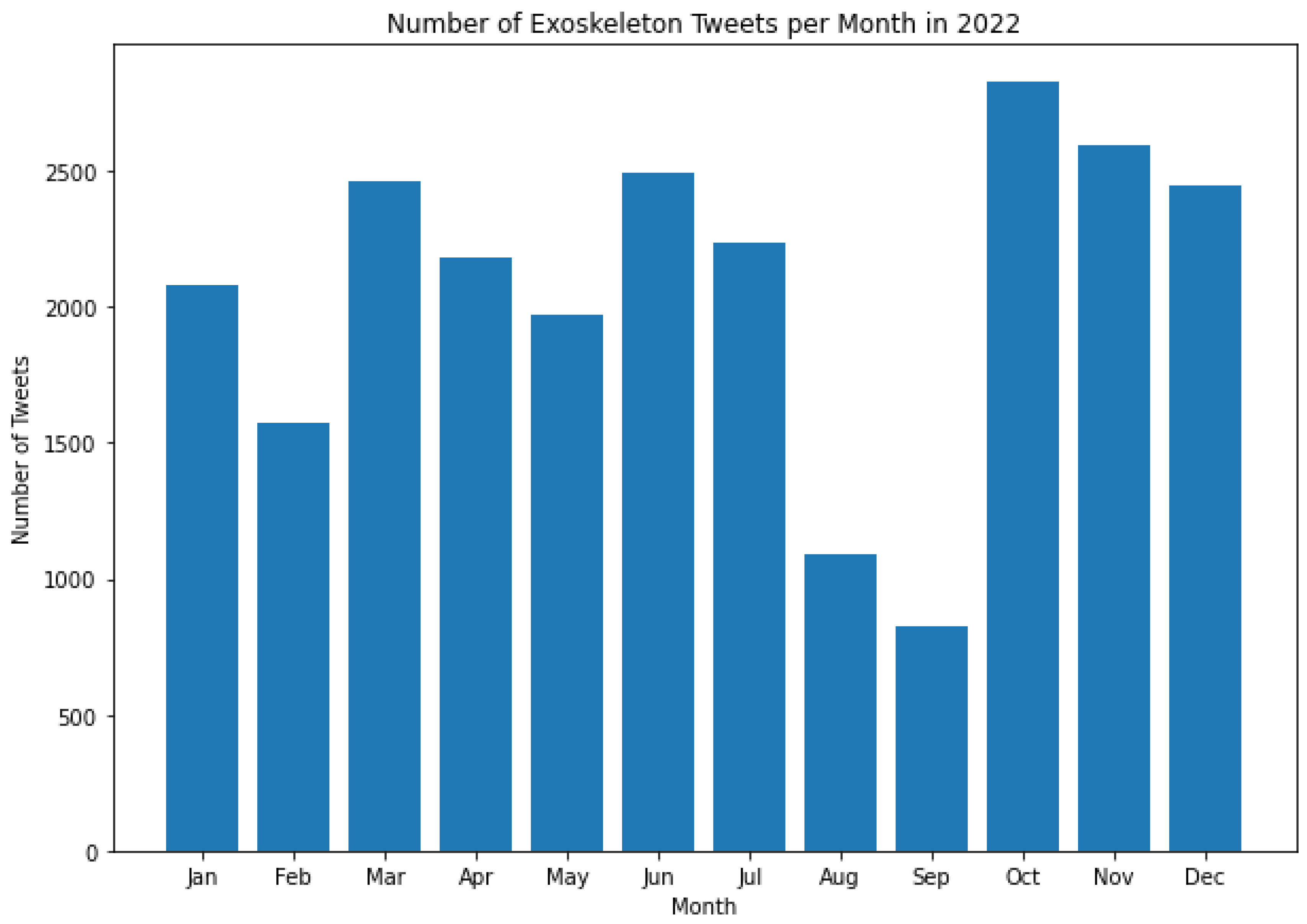
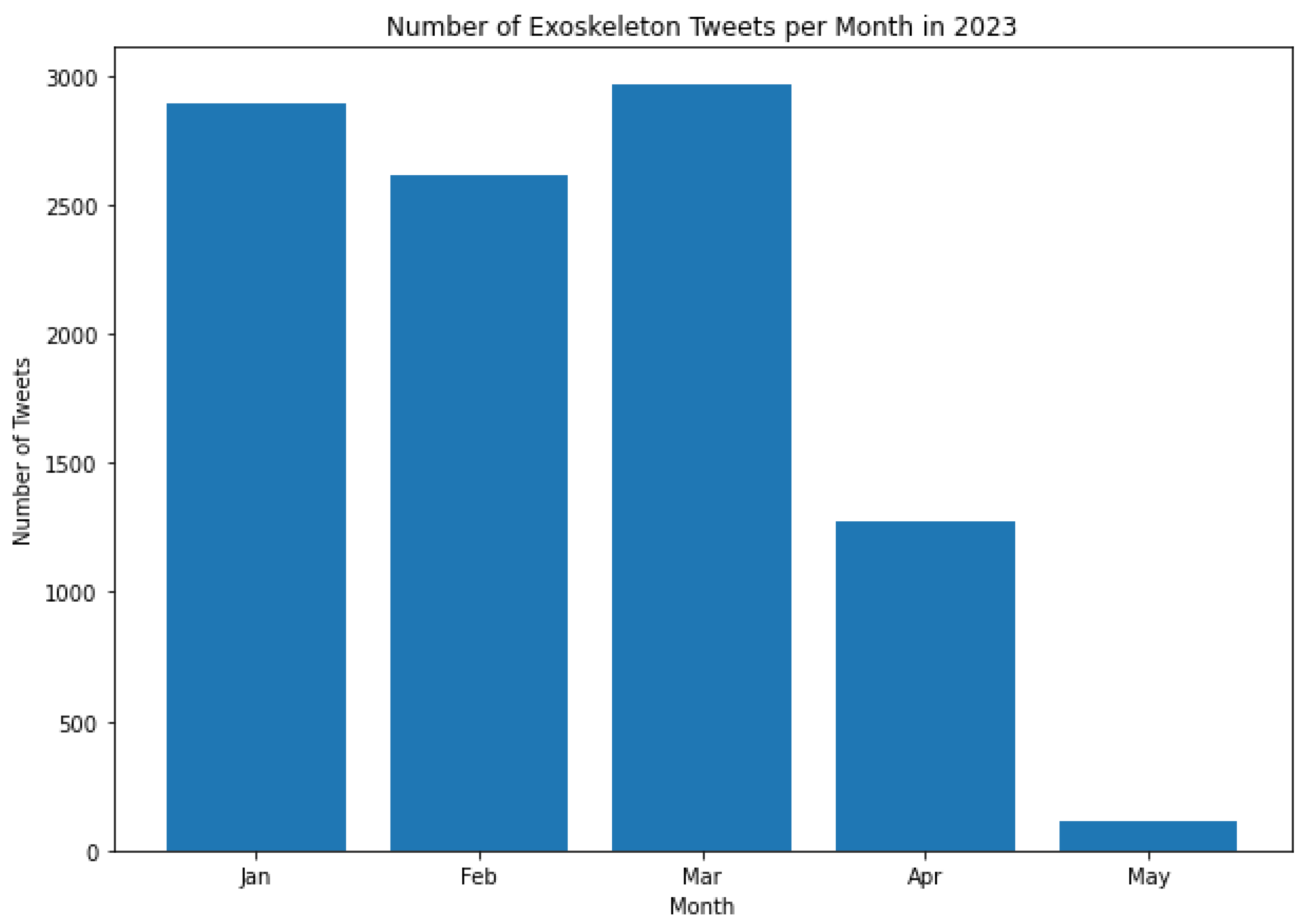
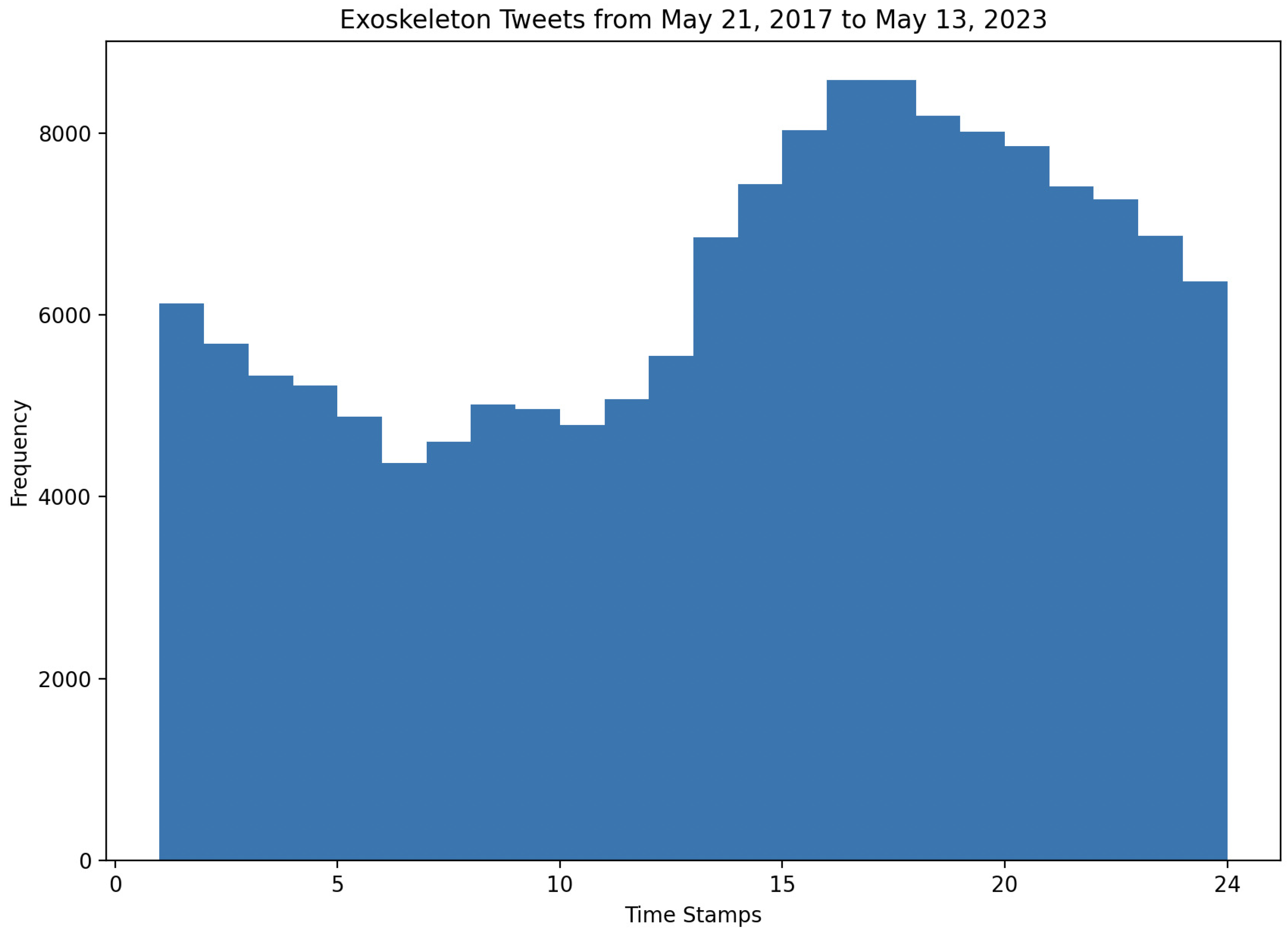
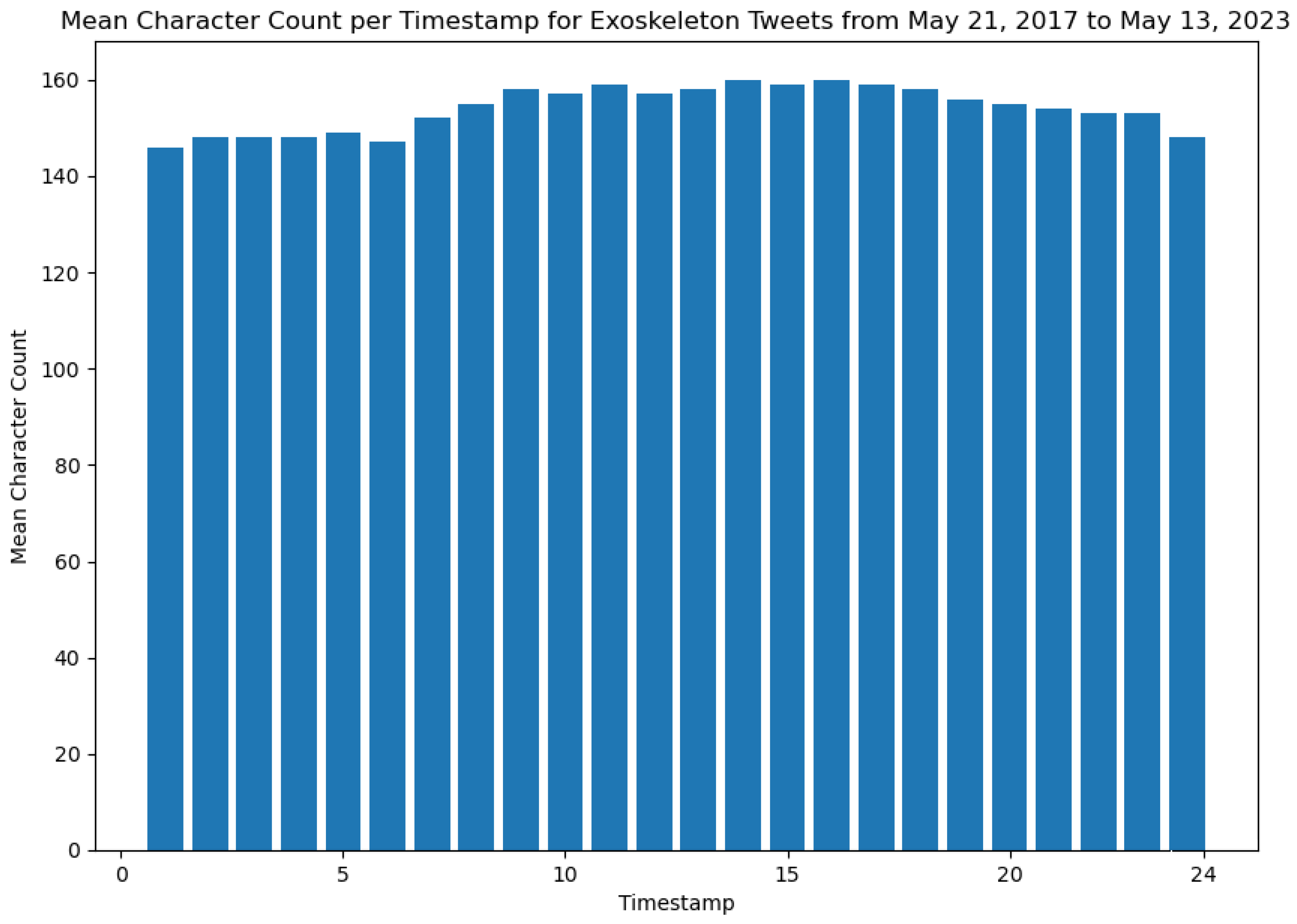
| Attribute Name | Description |
|---|---|
| Row no. | Row number of the data |
| Id | ID of the tweet |
| Created-At | Date and time when the tweet was posted |
| From-User | Twitter username of the user who posted the tweet |
| From-User-Id | Twitter User ID of the user who posted the tweet |
| To-User | Twitter username of the user whose tweet was replied to (if the tweet was a reply) in the current tweet |
| To-User-Id | Twitter user ID of the user whose tweet was replied to (if the tweet was a reply) in the current tweet |
| Language | Language of the tweet |
| Source | Source of the tweet to determine if the tweet was posted from an Android source, Twitter website, etc. |
| Text | Complete text of the tweet, including embedded URLs |
| Geo-Location-Latitude | Geo-Location (Latitude) of the user posting the tweet |
| Geo-Location-Longitude | Geo-Location (Longitude) of the user posting the tweet |
| Retweet Count | Retweet count of the tweet |
| Description | p-value |
|---|---|
| Number of Tweets per hour and the number of characters (mean) used in Tweets per hour | 0.0138 |
| Number of Tweets per hour and the number of characters (median) used in Tweets per hour | 0.0098 |
| Number of Tweets per hour and the number of hashtags used in Tweets per hour | 0.0006 |
| Number of Tweets per hour and the number of user mentions used in Tweets per hour | 2.44e-13 |
Disclaimer/Publisher’s Note: The statements, opinions and data contained in all publications are solely those of the individual author(s) and contributor(s) and not of MDPI and/or the editor(s). MDPI and/or the editor(s) disclaim responsibility for any injury to people or property resulting from any ideas, methods, instructions or products referred to in the content. |
© 2023 by the authors. Licensee MDPI, Basel, Switzerland. This article is an open access article distributed under the terms and conditions of the Creative Commons Attribution (CC BY) license (http://creativecommons.org/licenses/by/4.0/).


