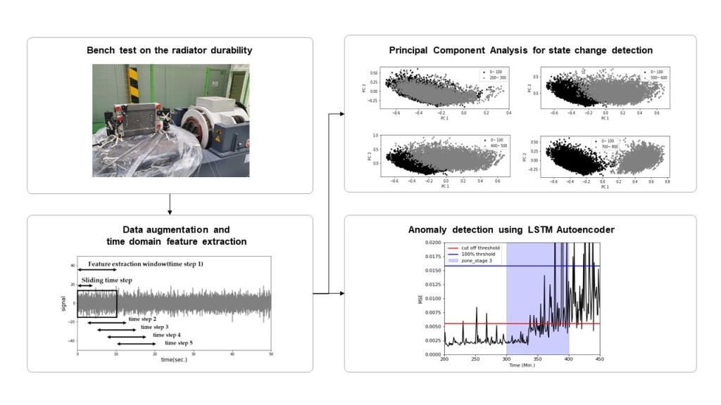
1. Introduction
This study discusses the application of Prognostics and Health Management (PHM) techniques [
1,
2,
3] to prevent radiator failures, enhance equipment availability, and consequently, reduce maintenance costs. The primary objective of PHM is to proactively detect early indicators of radiator malfunctions. In facilities and mechanical equipment powered by internal combustion engines, radiators play a pivotal role in preventing overheating. However, radiators operating in demanding environments face significant challenges, including temperature fluctuations and repetitive loads transferred from the machinery they serve. In such high-temperature or high-friction conditions, radiators may undergo temperature spikes beyond critical thresholds. Furthermore, mechanical damage can occur when the radiator's natural frequency resonates with the vibrations within the facility where it is installed. These resonant vibrations have the potential to induce cumulative fatigue failures in the welded joints of radiator material tubes.
Machine learning has significantly advanced the field of fault diagnosis by offering a range of algorithms capable of identifying abnormal conditions with high accuracy [
4]. Among various machine learning techniques, Gaussian Mixture Models (GMMs) are frequently used for clustering and density estimation tasks. These models have found applications in fault diagnosis to model normal behavior, thus aiding in the identification of anomalies [
5]. However, GMMs have limitations, such as their inability to capture temporal dependencies, making them less suitable for tasks requiring sequence-based learning [
6]. In contrast, Long Short-Term Memory (LSTM) networks, a type of recurrent neural network, excel in learning from sequences. These networks have shown promise in fault diagnosis and anomaly detection in time-series data [
7]. Nonetheless, LSTM is computationally intensive and are sensitive to hyperparameter settings [
8]. In industrial settings, particularly in the context of radiator fault diagnosis, anomaly detection is a critical tool for proactive maintenance [
10]. Existing methods often involve extensive manual feature extraction, making them less adaptive to new, unseen anomalies [
11]. These methods primarily suffer from an inability to adapt to new types of faults and insensitivity to early-stage anomalies. The requirement for manual labor in feature extraction remains a significant drawback [
12].
In light of the current advancements and identified limitations of LSTM as discussed based on above literature, this study aims to enhance the fault diagnosis process for radiators and related equipment. The approach chosen in this study combines GMM and LSTM to compensate for the shortcomings of LSTM and aims to balance the methods. This combination is tailored to address the challenges associated with diagnosing radiator faults in high-temperature or high-friction environments. Consequently, this study aims to improve equipment availability, prevent catastrophic failures, and significantly reduce maintenance costs. In doing so, this study fills existing technological gaps by adopting a combination approach that leverages GMMs for initial classification and LSTMs for sequence-based learning. GMMs are chosen for their strong clustering capabilities, useful for diagnosing known types of faults, while LSTMs are employed to capture the temporal sequences in data, thereby offering advanced anomaly detection for unknown or new types of radiator faults. In this study, both unsupervised learning models, GMM and LSTM autoencoder, were employed for radiator fault diagnosis. The choice of these two particular machine learning models is motivated by their complementary strengths: GMM excels at initial fault classification based on its clustering capabilities, while LSTM specializes in capturing time-dependent sequences, allowing for the advanced detection of unknown or new types of radiator fault.
In the subsequent sections, a comprehensive breakdown of the proposed methodology unfolds, commencing with:
Section 2 - Analyzing the Effects of Vibration on Radiator Integrity: In this section, an in-depth analysis of frequency response signals obtained from a real operational facility is undertaken to simulate the impact of vibrations on the structural integrity of radiators. A randomized durability vibration bench test is conducted, employing state-of-the-art acceleration sensors for real-time signal capture. The rationale behind the selection of GMM and LSTM autoencoders for fault diagnosis is elaborated upon.
Section 3 - Feature Engineering and Data Refinement: This section is dedicated to the critical task of feature engineering. Here, the focus is on extracting time-domain statistical features from raw data, refining them through PCA. The insights gained from PCA guide the subsequent training of the GMM. Findings related to fault diagnosis for stages 2 and 4, along with an in-depth exploration of anomaly detection for the unlabeled stage 3, are presented.
Section 4 - Leveraging LSTM Autoencoders: In this section, attention turns to the practical implementation of LSTM autoencoders for fault diagnosis and anomaly detection. The advantages of this approach are highlighted, showcasing its superiority over traditional methods, especially when dealing with time-series data.
Section 5 - Evaluation and Technical Contributions: The final section provides a comprehensive evaluation of the proposed combination of GMM and LSTM autoencoders. Here, meticulous detailing of the technical contributions of the methodology to the field of machine learning for fault diagnosis is presented. Emphasis is placed on its capability for precise fault detection and anomaly prediction. The practical implications of this approach for real-world applications, such as enhancing equipment uptime, preventing critical failures, and minimizing maintenance costs, are explored.
By integrating the strengths of GMM and LSTM within a unified framework, this study addresses the existing technological gaps in radiator fault diagnosis. The approach stands as a robust, adaptable, and highly efficient solution poised to make significant contributions in the domain.
2. Radiator dataset and research objective
2.1. Random durability vibration bench test and dataset
The focus of this study is on fin-and-tube heat exchangers, commonly known as radiators. Specifically, the study centers on cross-flow heat exchangers in which coolant circulates laterally, either from left to right or vice versa. Such exchangers feature tanks situated on both ends, interconnected by tubes that facilitate coolant flow, as depicted in
Figure 1. A cooling fan aids in dissipating waste heat from these tubes into the ambient environment. Moreover, to increase the heat transfer surface area and thereby enhance cooling efficiency, fins are strategically placed between the tubes [
13].
The primary material comprising the tank-tube-fin assembly is an aluminum alloy, well-known for its excellent thermal conductivity and efficient cooling properties. Aluminum brazing techniques are used to securely join these individual components. Notably, radiator welds are susceptible to breakage, often due to equipment-induced vibrations. Such failures result in coolant leakage, leading to operational downtime and increased maintenance expenses.
Given the identified vulnerability of radiator welds and the resulting faults, this study conducted two targeted experiments to simulate and promptly address radiator degradation. Initially, the vibration signal from the equipment impacting the radiator was captured. This captured signal served as the load profile for a random durability vibration bench test. The Accelerated Life Test (ALT) method was employed, aiming to artificially hasten the life degradation of test specimens to bolster lifetime reliability predictions and to minimize test durations and sample requirements [14-18]. Specifically, ALT introduces more extreme conditions than those usually encountered, thereby shortening required test time and sample counts [14-18]. Random durability vibration tests are especially suited for ALT, as they allow for the simultaneous introduction of multiple sinusoidal vibration components, closely mimicking real-world conditions.
To further clarify the relevance of these experiments, it's important to understand that radiator failures generally manifest in one of two ways: either the radiator's natural frequency comes into resonance with the vibrations from the equipment, or failures occur at the material tube welds, where fatigue loads tend to accumulate. In line with this, vibration signals from the radiator were specifically gathered during bench tests to simulate and accelerate fatigue failure scenarios at these tube welds.
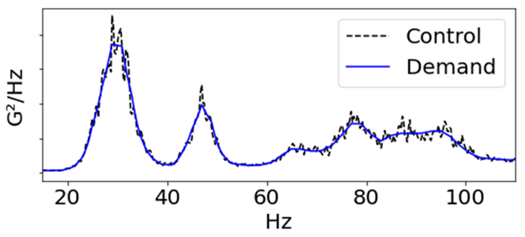
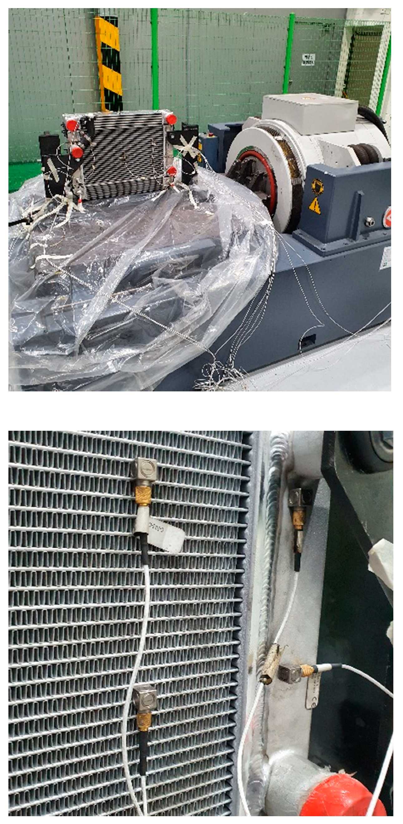
By analyzing the Power Spectral Density (PSD) of the vibration signal applied to the radiator, it was determined that fatigue failure of the radiator primarily occurred in the Y-axis direction. Consequently, a random durability vibration test was conducted, using the Y-axis PSD as the load profile (as shown in
Figure 2 and
Figure 3). PSD is a technique employed for analyzing the outcomes of a Fast Fourier Transform (FFT) on an acceleration response signal. In this process, the FFT output (G) is multiplied by a complex number component, generating real-number amplitudes (G
2). These amplitudes are then divided by the frequency resolution to produce a shape. Importantly, PSD is independent of the frequency resolution, making it advantageous for comparing vibration levels across signals. Due to these merits, PSD is often utilized to describe vibration characteristics in various random vibration specifications. Noteworthy standards for sinusoidal vibration testing include IEC 60068-2-6 [
19] and the U.S. military specification MIL-STD-810 [
20].
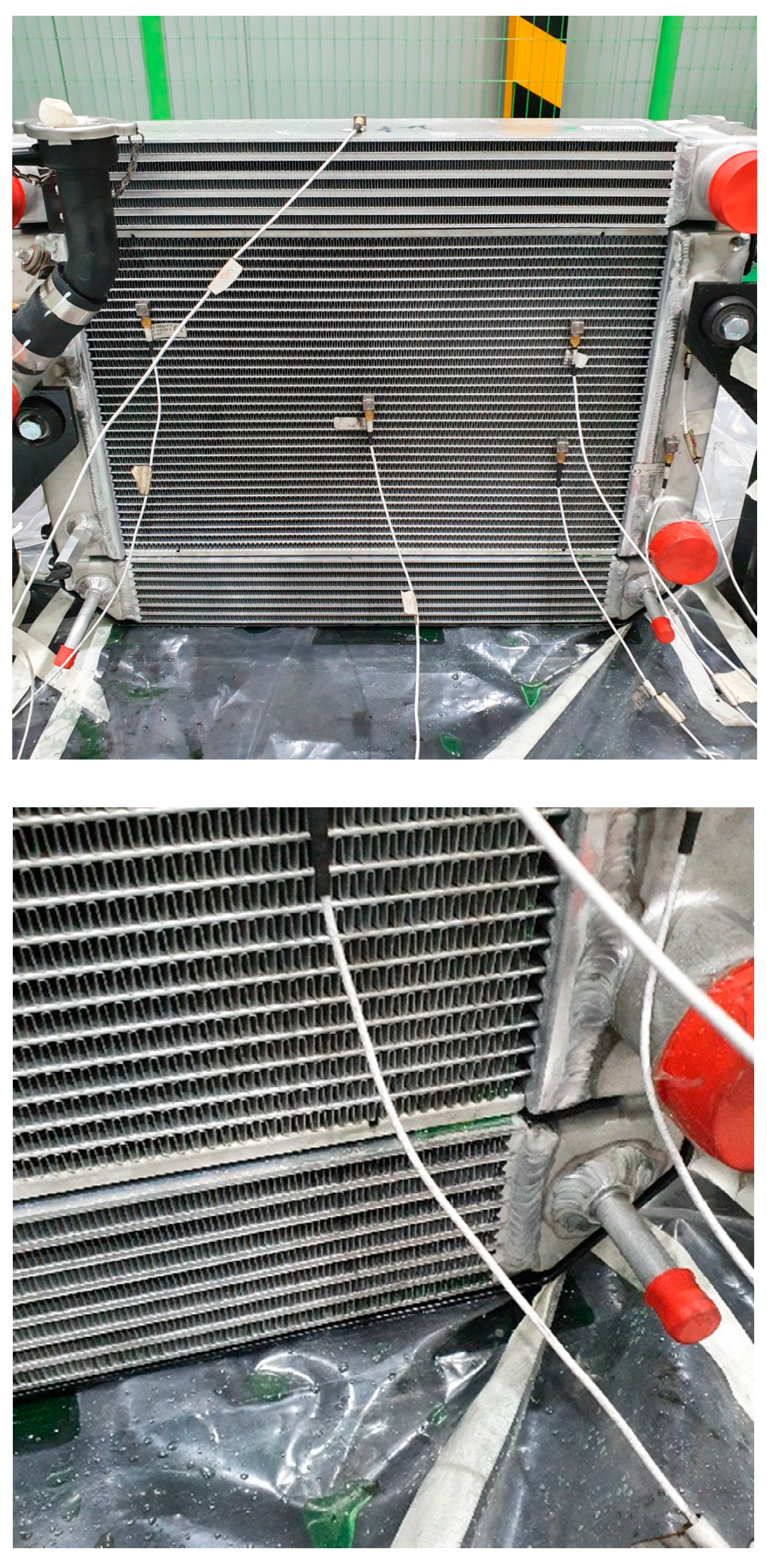
During the random durability vibration test, eight acceleration sensors were affixed to the radiator to capture signals at a rate of 12,800 Hz for a total test duration of 808 minutes. For the initial 300 minutes, the radiator showed no signs of damage. However, at around the 400-minute mark, a weld on the radiator tube fractured, leading to a minor coolant leak. As the test concluded, the radiator sustained severe damage, resulting in significant coolant leakage (see
Figure 4). The collected data were subsequently categorized and are detailed in
Table 1.
2.2. Methods and evluation metrics
Numerous studies have introduced a variety of classifiers for fault diagnosis, including but not limited to Neural Networks, Logistic Regression, Support Vector Machines (SVM), Random Forest, XGBoost, and LightGBM [21-26]. These classifiers typically operate under the constraints of supervised learning, requiring pre-classified abnormal data and labels for training. Acquiring such data from operational radiators in real-world settings presents significant challenges. Moreover, these classifiers are limited in their ability to identify new types of failures that have not been part of their training data. To address these limitations, this study employs unsupervised learning techniques, specifically Gaussian Mixture Models [27-28] and LSTM autoencoders [29-30], to classify data in stages 2 and 4. These models are capable of diagnosing faults during stage 3, the characteristics of which are not precisely known. When applied to real-world equipment, these models have the potential to detect both hidden and known failure modes, thereby improving diagnostic capabilities. Over time, the integration of these new failure cases and labels with existing supervised classifiers and expert knowledge is expected to enable more accurate and comprehensive fault diagnosis.
The performance of the chosen unsupervised models is evaluated using the Area Under the Curve (AUC) metric. This metric is particularly useful when data do not have clear demarcations between normal and abnormal conditions, and where precise threshold selection is challenging. The AUC quantifies the performance of a model without requiring a specific threshold and is calculated based on the Receiver Operating Characteristic (ROC) curve. This curve depicts the relationship between the True Positive Rate (TPR) and the False Positive Rate (FPR). A higher AUC score, ranging between 0 and 1, indicates better model performance. Specifically, a perfect classifier would achieve an AUC close to 1, while a random classifier would score around 0.5. Any performance falling below this threshold, resulting in an AUC less than 0.5, would be considered worse than random classification. The AUC score serves as the evaluation metric for the binary classification results of stages 2 and 4, based on the thresholds established during stage 1. Detailed diagnosis of unknown conditions in stage 3 is conducted using the thresholds of the trained unsupervised models.
3. GMM-based fault diagnosis
3.1. Feature engineering and PCA of radiator dataset
The dataset included eight acceleration signals, with each time series signal containing 620,544,000 data points, collected at a rate of 12,800 Hz for 808 minutes. Given the large volume of data, which could impede efficient analysis, feature engineering techniques were employed for data compression. Specifically, seven statistical features—minimum, maximum, absolute mean, variance, root mean square (RMS), skewness, and kurtosis—were extracted for each time window, ranging from one to ten seconds. This yielded 56 feature vectors, effectively transforming the data dimensions from 620,544,000×8×1 to 4,848×8×7 in a ten-second window. It should be noted that increasing the window size reduces the number of feature vectors. To augment the feature vectors and ensure sufficient training data, a sliding window technique was applied, as illustrated in
Figure 5, depicting the difference between the conventional and sliding window augmentation methods. This technique increased the number of ten-second feature vectors from 4,848 to 48,471.
Feature vectors derived from ten-second windows using a sliding window technique underwent dimensionality reduction through PCA. This led to observable state changes in the data. PCA serves as a method to minimize data dimensionality by generating new variables, known as principal components, which encapsulate the key information of the original dataset [
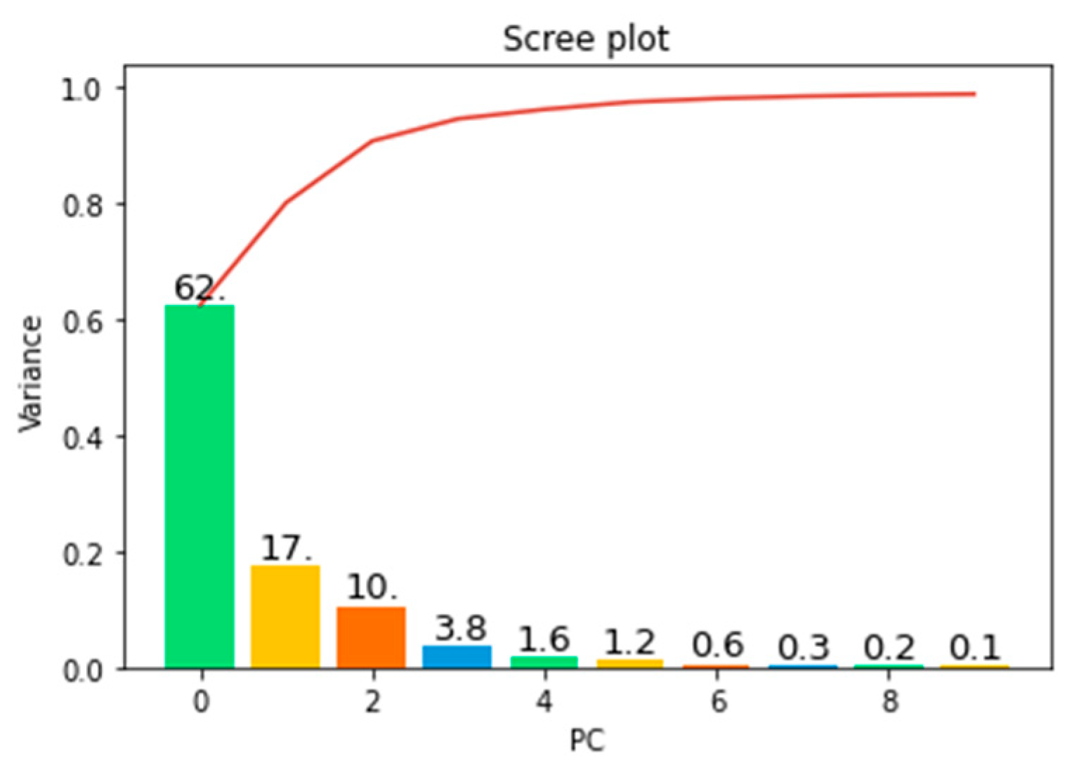
31]. A scree plot, along with a list of eigenvalues of these principal components in descending order, was analyzed to determine the optimal number of components for data representation (shown in
Figure 6). The scree plot serves as a vital tool for assessing the impact of PCA on the dataset and indicating the appropriate number of principal components [
32]. In this study, the first principal component was identified as a linear combination of variables accounting for the maximum variance, whereas the second principal component, geometrically orthogonal to the first, explained the next highest variance. The analysis indicated that the first and second principal components collectively accounted for 62% and 17% of the data variance, respectively, explaining 89% of the total variance.
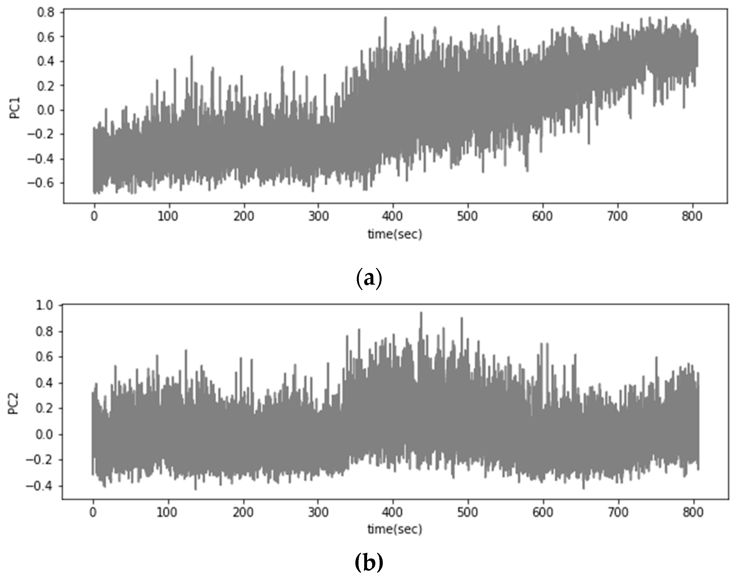
As depicted in
Figure 7, a time-series graph visualizing the first and second principal components (PC1 and PC2) was generated. The graph depicted a gradual temporal rise in the values of PC1, but this increase was accompanied by notable fluctuations, making it challenging to accurately discern state changes. Likewise, PC2 also displayed substantial fluctuations, further complicating the visual differentiation between normal and abnormal data distributions.
Building on the limitations of the time-series graph discussed in
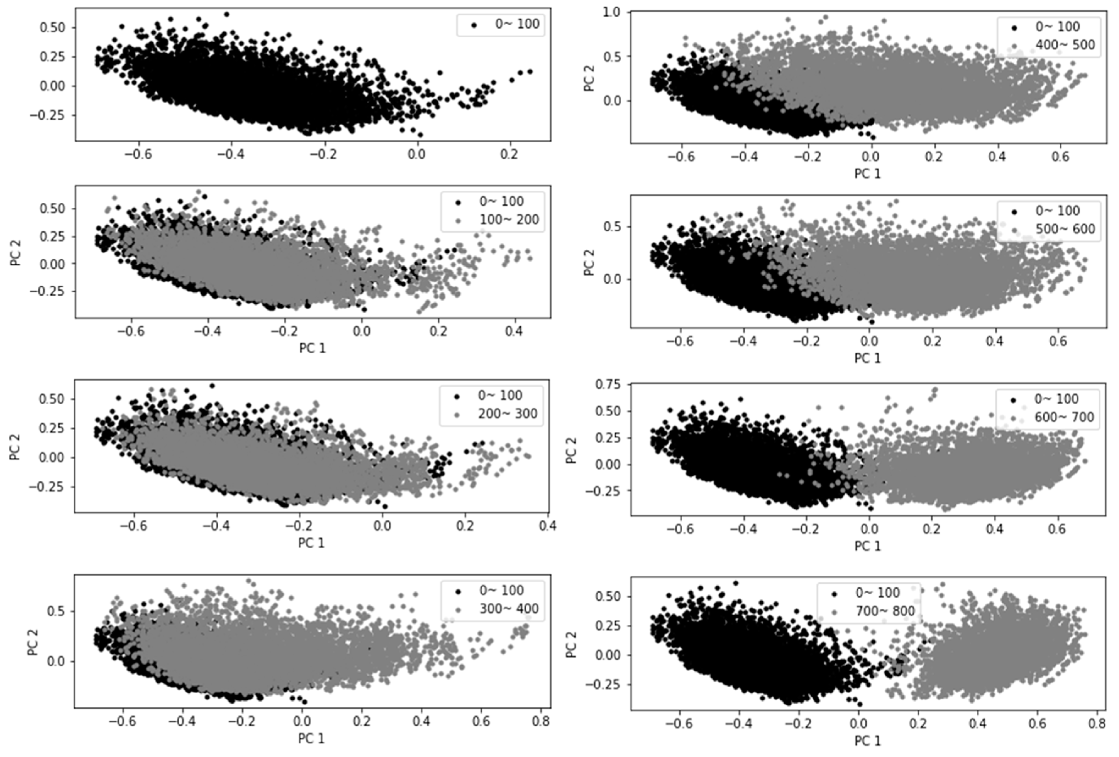
Figure 7, a two-dimensional scatter plot was generated to further investigate the values of PC1 and PC2. As illustrated in
Figure 8, a two-dimensional scatter plot was generated to visualize the values of PC1 and PC2. This visualization revealed changes in the state of the cluster when compared to the normal state observed during stage 1 (0–100 minutes). However, data from stage 3 (300–400 minutes), where radiator failure was anticipated, showed considerable overlap with stage 1. A similar overlap was observed with data up to 600 minutes in stage 4. Nonetheless, the data representing the end-failure portion of the experiment displayed distinct characteristics compared to the normal state data.
In light of the challenges noted in the time-series visualization in
Figure 7, a two-dimensional scatter plot of PC1 and PC2 was generated, as illustrated in
Figure 8. This approach allowed for a more detailed observation of cluster state changes in comparison to the normal state observed during stage 1 (0–100 minutes). However, it was found that the data from stage 3 (300–400 minutes), where radiator failure was expected, showed considerable overlap with stage 1. Similar overlap was also seen in the data up to 600 minutes in stage 4. Despite these overlaps, the data corresponding to the end-failure part of the experiment displayed distinct characteristics compared to the normal state data.
Given the complexities observed in
Figure 7 and
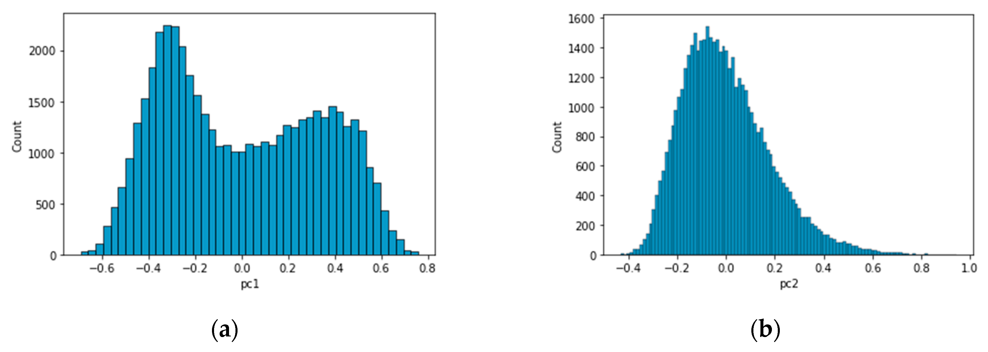
Figure 8, a histogram analysis of principal components 1 and 2 was also conducted, as depicted in
Figure 9. This analysis revealed that PC1 exhibited a bimodal distribution with two distinct peaks, while PC2 showed a unimodal distribution with a single peak. Typically, a bimodal distribution indicates the presence of two different underlying distributions, each with its own set of characteristics or mean values. In this case, the bimodal nature of PC1 is believed to represent a mixture of data from both normal and abnormal states.
3.2. Fault Diagnosis and anomaly detection result using GMM
Building upon the histogram analysis that revealed a bimodal distribution for PC1, this section investigates the application of Gaussian Mixture Models for classifying normal and abnormal data. Utilized as an unsupervised learning method, GMM employs probabilistic modeling to represent intricate datasets as amalgamations of simpler probability distributions. The GMM model describes data as the sum of multiple Gaussian distributions and assumes that the data is organized into multiple clusters. The GMM estimates the mean and covariance matrix of the Gaussian distributions for each cluster and assigns data points to clusters by calculating the probability of the data belonging to each cluster. By calculating the probability of each cluster for all data points, the data was assigned to the cluster with the highest probability. Accordingly, the GMM can be used effectively even when the distributions are mixed or overlapping. Therefore, even in cases where the data consists of several different Gaussian distributions, the GMM can be used to model the data.
To optimize the GMM, the Expectation-Maximization (EM) algorithm is employed to minimize the negative log-likelihood during the learning process, as cited in [
33]. In the context of GMM, the EM algorithm estimates the model parameters, specifically the mean and covariance of each Gaussian distribution that constitutes the model. The log-likelihood serves as an indicator of how well the model fits the data. A higher log-likelihood value signifies a better fit of the model to the data. GMM aims to minimize the negative value of the log-likelihood during the training phase. This approach is commonly taken in optimization problems because minimization is often computationally more tractable than maximization. Consequently, a higher absolute value of the negative log-likelihood would suggest that the data point is not well-represented by the model. Given a dataset
and model parameters
, the log-likelihood is expressed as follows:
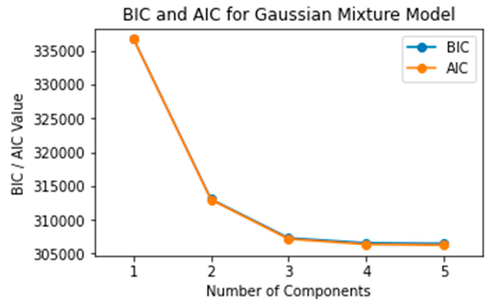
Two or more Gaussian distributions were determined based on the analysis results of PC1. The GMM was trained with the overall data of PC1 and PC2 from stages 1 to 4. Before initiating fault diagnosis, the number of Gaussian components in the GMM was carefully evaluated by varying the component count from 1 to 5. The Bayesian Information Criterion (BIC) and Akaike Information Criterion (AIC) were employed to assess the model fit for each distribution. A poorly chosen number of Gaussians can lead to model overfitting, thus compromising its reliability and predictive power. BIC and AIC serve as key metrics in model selection, balancing fit and complexity, as cited in [
34]. BIC is particularly focused on accommodating uncertainties and is defined as follows:
where,
represents the number of parameters in the model. In the context of GMM, the mean and covariance are parameters for each Gaussian distribution, so the value of
is contingent on the number of Gaussian distributions incorporated in the model.
denotes the total number of samples present in the dataset. The Akaike Information Criterion serves as another model selection criterion and is mathematically defined as follows:
In model selection, the Bayesian Information Criterion and Akaike Information Criterion are often employed to balance goodness-of-fit with model complexity. BIC incorporates a penalty term that is more stringent compared to AIC, hence favoring simpler models when the fit is comparable. As revealed in
Figure 10, both BIC and AIC values exhibit a declining trend with an increasing number of Gaussian distributions. However, the rate of this decline begins to stabilize when the model incorporates three or more Gaussian distributions. In light of this, based on the BIC and AIC criteria, the optimal number of Gaussian distributions was determined to be at least three.
In light of the observation from BIC and AIC analysis, an exploratory study was carried out to assess how the choice of the number of Gaussian distributions affects fault diagnosis outcomes. Moreover, the sensitivity of the diagnostic results to the feature engineering window size was also investigated, varying the window from one to ten seconds. The fault diagnosis process is delineated as follows:
Train the Gaussian Mixture Model.
Establish a threshold value based on the absolute log-likelihood distribution derived from stage 1.
In stages 2–4, data points whose absolute log-likelihood values exceed the predetermined threshold are flagged as faulty.
As outlined in
Table 2, a binary classification was conducted for stages 2 and 4 to distinguish between normal and abnormal conditions. Consistent with the BIC and AIC findings, Area Under the Curve (AUC) scores reached a stable level when employing three or more Gaussian components. Moreover, an incremental gain in AUC was observed with an increase in the feature engineering window size. However, extending the sliding window technique to a ten-second frame did not result in any further improvement in the AUC metric.
For a detailed diagnosis in the unlabeled stage 3 area, anomaly detection was conducted employing two specific methods:
Feature Engineering: Utilized a ten-second window combined with sliding window augmentation.
Gaussian Distributions: Set to three, based on both the BIC and AIC analysis and expert understanding of fault diagnosis.
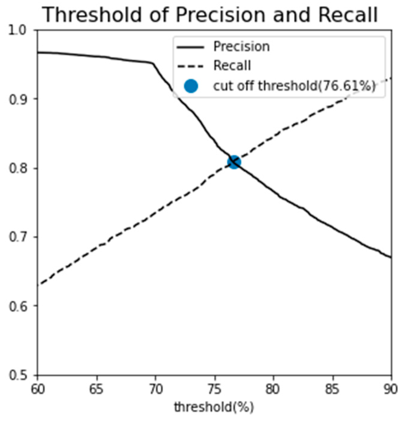
The number of Gaussian distributions was finalized at three, guided by both the BIC and AIC analyses as well as domain-specific expertise in fault diagnosis. The classification objective was to delineate the data into three categories: normal, semi-fault, and fault states. The choice of classification threshold is crucial as it affects the balance between precision and recall, metrics that are often inversely proportional to each other. A threshold set at 100% (indicating near-perfect recall) is prone to false negatives, potentially misclassifying abnormal data points as normal. Conversely, a lower threshold optimizes for precision at the expense of recall, increasing the likelihood of mislabeling normal instances as abnormal. Given that outliers exist even within the log-likelihood distribution of the stage 1 normal data, a 100% threshold would erroneously label all outliers as normal, thereby increasing the risk of missing a critical radiator fault. To mitigate both over-detection and under-detection, an optimal threshold was sought by examining the relationship between precision and recall at various thresholds. The intersection point of these two metrics was selected as the cut-off, resulting in a threshold value of 76.61%, as shown in
Figure 11.
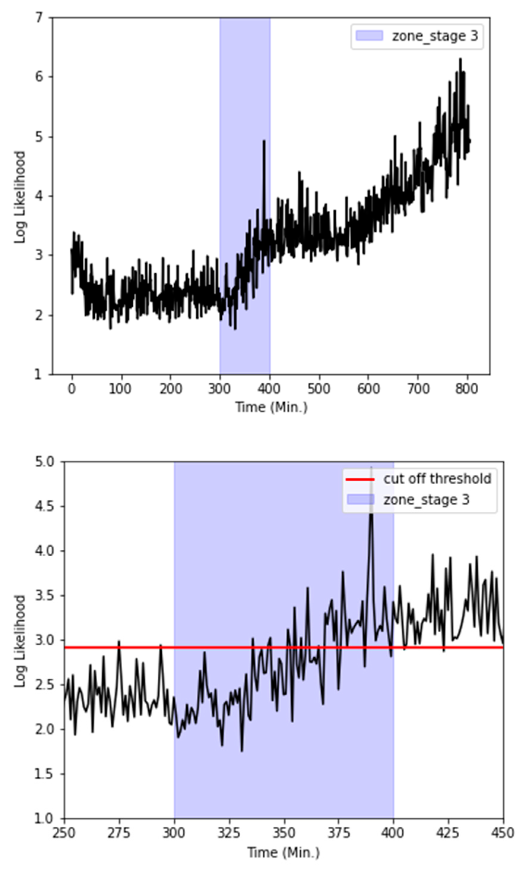
To examine temporal variations in the radiator state, the absolute log-likelihood values for all stages (1–4) were averaged in 60-second intervals, as illustrated in the left pane of
Figure 12. During stage 1, the log-likelihood value exhibited an initial decrease before reaching a stable plateau. However, commencing at approximately 300 minutes, a noticeable upward trend was observed in the absolute values of the log-likelihood. This escalation crossed the established cut-off threshold at around the 400-minute mark, coinciding with the visual confirmation of a coolant leak.
Additionally, a focused analysis of stage 3, displayed in the right pane of
Figure 12, revealed recurrent excursions of the absolute log-likelihood values beyond the cut-off threshold, starting at roughly 350 minutes. This pattern is indicative of a deteriorating radiator condition.
4. LSTM Autoencoder-based fault diagnosis
4.1. Rationale for LSTM Autoencoder selection
An autoencoder serves as a specialized type of neural network designed to leverage unlabeled data. The architecture typically includes an encoder, responsible for mapping the input (
) into an internal representation, and a decoder, tasked with reconstructing the output (
) from this internal representation. The output, often referred to as a "reconstruction," serves as an approximate replica of the input. The model is generally trained using Mean Squared Error (MSE) that is representing the measure of the average squared difference between predicted values (
) and actual values (
) to quantify the reconstruction loss as follows:
LSTM networks are designed to address the vanishing gradient problem that hampers traditional Recurrent Neural Networks (RNNs) [
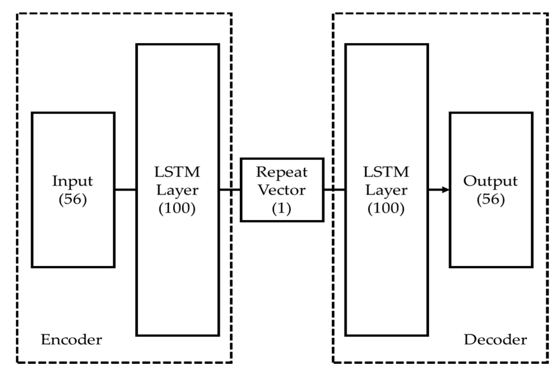
36]. This challenge is especially acute in deep networks with multiple layers and nodes. In such cases, the initial layers are often inadequately trained, a problem that worsens as the length of the training sequence increases. This leads to gradients that approach zero during the backpropagation process [37-38]. Unlike traditional RNNs, LSTMs effectively circumvent the vanishing gradient issue by incorporating both long-term and short-term state variables into the learning algorithm. This enables LSTMs to achieve successful training even over extensive data sequences, thus resolving the long-term dependency problem often found in standard RNNs [39-40]. In this study, an LSTM autoencoder was implemented, consisting of two LSTM layers specifically designed for handling time-series data, as illustrated in
Figure 13. Each of these layers serves both as an encoder and a decoder within the network architecture [
41]. A "repeat vector" is utilized to resize the compressed latent space representation back to the original sequence length. This allows the decoder to use the compressed representation multiple times, aiding in a more precise reconstruction of the original input sequence.
As outlined in
Section 3, GMMs were trained on the entire dataset spanning stages 1 to 4. Thresholds for fault diagnosis were derived from the absolute log-likelihood distribution of stage 1 data. While this approach allows for effective post-hoc analysis, it may not be well-suited for proactive fault diagnosis. To address this limitation,
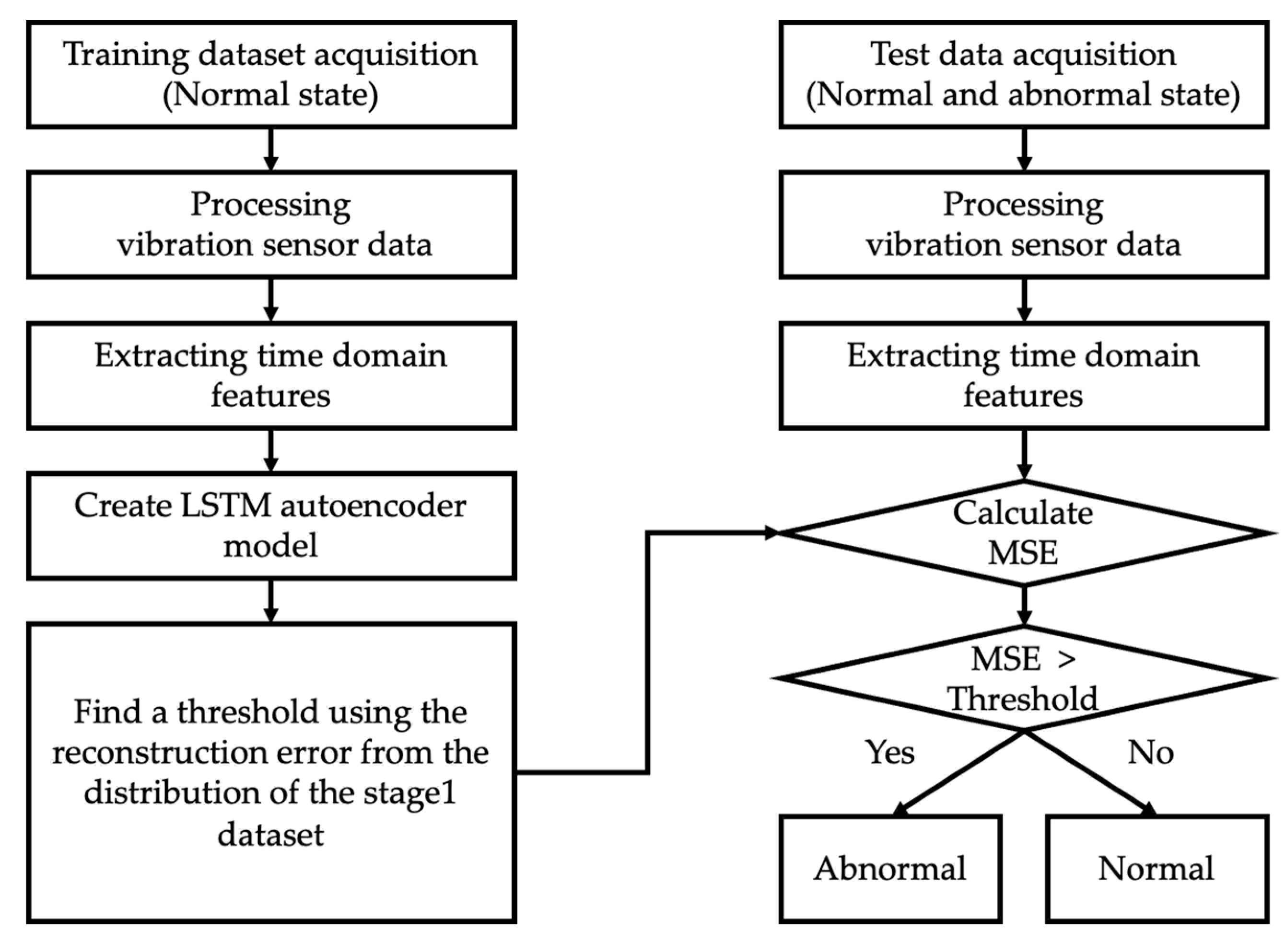
Figure 14 introduces an LSTM autoencoder-based fault diagnosis algorithm. A previous set comprising 56 feature vectors served as the training dataset. The LSTM autoencoder was initially trained on stage 1 data, which consists exclusively of normal states. A threshold was determined from the Mean Squared Error distribution of the stage 1 training data. If the MSE for data from stages 2 to 4 falls below this threshold, the state is classified as normal; if it exceeds the threshold, the state is considered abnormal. Additionally, MSE was employed as a fault level index, offering an intuitive visual representation of the radiator's degradation process.
4.2. Fault diagnosis and anomaly detection result using LSTM Autoencoder
In line with the GMM analysis, the appropriate window size was examined, ranging from one to ten seconds for feature engineering. Additionally, a sliding augmentation method was applied to the ten-second window to increase the number of data points. When evaluating the model's performance, experiments were conducted by varying the number of nodes in the LSTM hidden layer for the Autoencoder. Furthermore, the dropout rate was adjusted to mitigate overfitting [
42], and the L2 regularization parameter was modified to assess its impact on performance [
43]. The experimental results, as summarized in
Table 3, revealed that the AUC score for fault diagnosis exhibited a gradual improvement with an increasing window size for feature engineering. Moreover, the utilization of the sliding augmentation technique led to an enhancement in the AUC score, increasing it from 0.9728 to 0.9893. Furthermore, an increase in the number of nodes in the hidden layer also resulted in an improved AUC score. Conversely, a decline in the AUC score was observed when dropout and L2 regularization were applied.
Similar to the GMM analysis, a comprehensive diagnosis of the unlabeled stage 3 area involved anomaly detection using three methods:
Feature engineering method: A 10-second window with sliding augmentation.
LSTM AE structure: Configured as 100/1/100.
Dropout and L2 Regularization: Not applied.
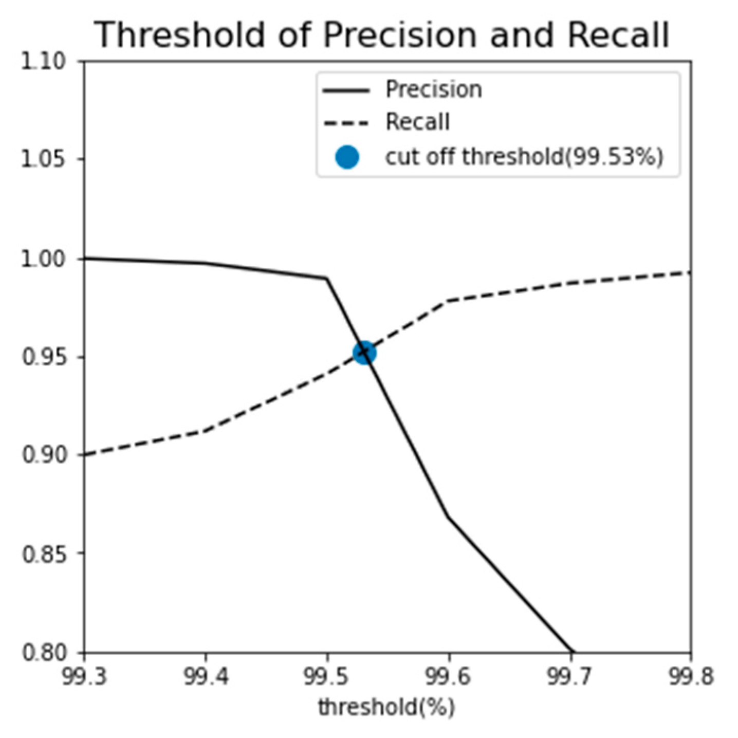
To establish an appropriate MSE threshold and minimize both over-detection and under-detection, an intersection point was determined by analyzing the correlation between precision and recall at various threshold values. This analysis yielded a threshold of 99.53%, as illustrated in
Figure 15. Consequently, it was determined that a threshold of approximately 99.53% was necessary for diagnosing radiator faults.
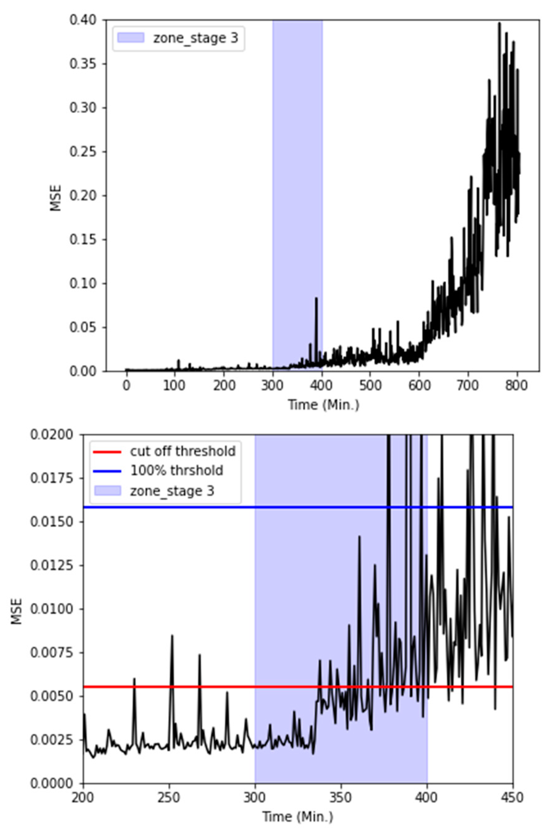
The MSE values for all stages 1-4 were averaged every 60 seconds to track changes in the radiator's condition over time, as depicted in the left side of
Figure 16. The MSE magnitude exhibited a gradual increase as time progressed. Notably, the MSE values crossed the cut-off threshold at approximately 400 minutes, which coincided with the visual confirmation of a coolant leak.
Additionally, as shown on the right side of
Figure 16, during stage 3, the MSE was observed to repeatedly surpass the cut-off threshold around the 335 to 340-minute mark, indicating radiator failure. This observation closely aligned with the GMM results, which also pinpointed the onset of radiator issues at around 350 minutes.
5. Discussion
In this study, fault diagnosis for radiators was conducted using both GMM and LSTM autoencoder models. Initially, the radiator underwent a random durability vibration bench test to accelerate vibration-induced failure and acquire acceleration signals. The vibration data was divided into stages 1–4, and time-domain statistical features were extracted for efficient data analysis using a one- to ten-second window for feature engineering. Additionally, the feature vector was augmented by applying a sliding technique to ten-second windows.
The appropriate number of principal components was determined, and two principal components were trained on the GMM. Additionally, the GMM was employed to establish thresholds based on the absolute log-likelihood distribution of stage 1 for diagnosing faults in stages 2 and 4. The GMM model achieved a maximum AUC of 0.9009. The cut-off threshold was set at the point of intersection between precision and recall. Using this threshold, anomaly detection in stage 3 enabled the diagnosis of faults in the unlabeled state. However, it's worth noting that different distributions were observed even within the normal state of the training data. Achieving an AUC score higher than 0.9 when performing fault diagnosis using the stage 1 threshold proved challenging.
The GMM-based fault diagnosis had a limitation in that the entire dataset encompassing stages 1 to 4 was trained collectively. Consequently, GMM wasn't suitable for predicting faults in advance. To address this, a fault diagnosis algorithm was developed utilizing an LSTM autoencoder, which was exclusively trained on the normal state data from stage 1. This approach aimed to avoid the need for post-fault event diagnosis. Thresholds were extracted from the MSE distribution observed in stage 1, and fault diagnosis was subsequently conducted in stages 2 and 4. The experimental results demonstrated that this algorithm achieved a maximum AUC of 0.9912. Similar to the GMM, anomaly detection was performed in the unlabeled stage 3 using the cut-off point where precision and recall intersect. Furthermore, an additional analysis was carried out using the 100%-point threshold from the stage 1 MSE distribution, which closely approximates the cut-off point. Setting the threshold at 100% resulted in similar time frames for fault occurrence and alarm generation. In such scenarios, the potential for higher opportunity costs and reduced equipment productivity due to reactive maintenance could be anticipated. Conversely, adopting the cut-off threshold as the fault alarm criterion enables earlier radiator maintenance, minimizing the opportunity cost associated with equipment downtime and ensuring effective radiator maintenance.
This study has demonstrated an approach to enhance the accuracy of product reliability life assessment in Accelerated Life Tests. The investigation focused on radiator fault diagnosis through the adjustment of thresholds using the absolute log-likelihood distribution of the GMM and the reconstruction error distribution of the LSTM autoencoder model. In the future, it is possible to achieve efficient radiator maintenance by utilizing the log-likelihood and MSE as fault level indicators and optimizing the balance between equipment lead time and opportunity cost through the establishment of appropriate radiator maintenance thresholds. Additionally, there is potential for universal application of outlier detection and fault diagnosis using the LSTM autoencoder, with training exclusively on normal state datasets. Furthermore, the fault diagnosis process can be further refined through the integration of updated fault cases and labels, existing supervised classifiers, and expert knowledge following hidden failure detection.
Author Contributions
Conceptualization and methodology, J.-G.L.; validation, formal analysis and investigation, J.-G.L., D.-H.K. and J.H.L.; data curation, J.-G.L. and J.H.L.; research administration, J.H.L.; funding acquisition, J.H.L. All authors have read and agreed to the published version of the manuscript.
Funding
This work was supported by the 'Autonomous Ship Technology Development Program (20011164, Development of Performance Monitoring and Failure Prediction, and Diagnosis Technology for Engine System of Autonomous Ships)' funded by the Ministry of Trade, Industry & Energy (MOTIE, Korea).
Institutional Review Board Statement
Not applicable.
Informed Consent Statement
Not applicable.
Data Availability Statement
In accordance with company security policies, the data presented in this study are available upon request from the corresponding author. The data derived from the present study are only partially available for research purposes.
Conflicts of Interest
The authors declare no conflict of interest.
References
- Tsui, K.L.; Chen, N.; Zhou, Q.; Hai, Y.; Wang, W. Prognostics and health management: A review on data driven approaches. Mathematical Problems in Engineering 2015. [CrossRef]
- Lee, J.; Wu, F.; Zhao, W.; Ghaffari, M.; Liao, L.; Siegel, D. Prognostics and health management design for rotary machinery systems—Reviews, methodology and applications. Mechanical systems and signal processing 2014, 42, 314–334. [Google Scholar] [CrossRef]
- Meng, H.; Li, Y.F. A review on prognostics and health management (PHM) methods of lithium-ion batteries. Renewable and Sustainable Energy Reviews. 2019, 116, 109405. [Google Scholar] [CrossRef]
- Lei, Y.; Yang, B.; Jiang, X.; Jia, F.; Li, N.; Nandi, A.K. Applications of machine learning to machine fault diagnosis: A review and roadmap. Mechanical Systems and Signal Processing. 2020, 138, 106587. [Google Scholar] [CrossRef]
- Cao, S.; Hu, Z.; Luo, X.; Wang, H. Research on fault diagnosis technology of centrifugal pump blade crack based on PCA and GMM. Measurement. 2021, 173, 108558. [Google Scholar] [CrossRef]
- Chen, Z.; Peng, Z.; Zou, X.; Sun, H. Deep learning based anomaly detection for muti-dimensional time series: A survey. In China Cyber Security Annual Conference. July 2021; pp. 71–92.
- Zhao, H.; Sun, S.; Jin, B. Sequential fault diagnosis based on LSTM neural network. Ieee Access. 2018, 6, 12929–12939. [Google Scholar] [CrossRef]
- Yu, Y.; Si, X.; Hu, C.; Zhang, J. A review of recurrent neural networks: LSTM cells and network architectures. Neural computation. 2019, 31, 1235–1270. [Google Scholar] [CrossRef]
- Janiesch, C.; Zschech, P.; Heinrich, K. Machine learning and deep learning. Electronic Markets. 2021, 31, 685–695. [Google Scholar] [CrossRef]
- Kamat, P.; Sugandhi, R. Anomaly detection for predictive maintenance in industry 4.0-A survey. In E3S web of conferences. 2020; Vol. 170, p. 02007.
- Chalapathy, R.; Chawla, S. Deep learning for anomaly detection: A survey. arXiv preprint arXiv:1901.03407. 2019. arXiv:1901.03407. 2019.
- Dara, S.; Tumma, P. Feature extraction by using deep learning: A survey. In 2018 Second international conference on electronics, communication and aerospace technology (ICECA). March 2018; pp. 1795–1801.
- Bergman, T. L.; Lavine, A. S.; Incropera, F. P.; DeWitt, D. P. Introduction to heat transfer, 5th ed. John Wiley & Sons, pp.632-633, 2005.
- Klyatis, L.M. Accelerated reliability and durability testing technology, Vol. 70, John Wiley & Sons, 2012.
- Elsayed, E.A. Overview of reliability testing. IEEE Transactions on Reliability. 2012, 61, 282–291. [Google Scholar] [CrossRef]
- Kapur, K. C.; Pecht, M. Reliability engineering, Vol. 86, John Wiley & Sons, 2014.
- O'Connor, P.; Kleyner, A. Practical reliability engineering. John Wiley & Sons, 2012.
- Zio, E. Reliability engineering: Old problems and new challenges. Reliability engineering & system safety. 2009, 94, 125–141. [Google Scholar]
- IEC. IEC 60068-2-6: Environmental testing - Part 2-6: Tests - Test Fc: Vibration (sinusoidal). IEC, 2011.
- MIL-STP-810. Environmental Engineering Considerations and Laboratory Tests. no date.
- Breiman, L. Random forests. Machine learning. 2001, 45, 5–32. [Google Scholar] [CrossRef]
- Ke, G.; Meng, Q.; Finley, T.; Wang, T.; Chen, W.; Ma, W.; Ye, Q.; Liu, T.Y. Lightgbm: A highly efficient gradient boosting decision tree. Advances in neural information processing systems 2017, 30. [Google Scholar]
- Breiman, L.; Friedman, J.; Stone, C.J.; Olshen, R.A. Classification and regression trees. CRC press. 1984.
- Chen, T.; Guestrin, C. Xgboost: A scalable tree boosting system. In Proceedings of the 22nd acm sigkdd international conference on knowledge discovery and data mining, August 2016; pp. 785–794.
- Noble, W.S. What is a support vector machine? Nature biotechnology. 2006, 24, 1565–1567. [Google Scholar] [CrossRef]
- Dreiseitl, S.; Ohno-Machado, L. Logistic regression and artificial neural network classification models: a methodology review. Journal of biomedical informatics. 2002, 35, 352–359. [Google Scholar] [CrossRef]
- Reynolds, D.A. Gaussian mixture models. Encyclopedia of biometrics. 2009, 741, 659–663. [Google Scholar]
- Rasmussen, C. The infinite Gaussian mixture model. Advances in neural information processing systems. 1999, 12. [Google Scholar]
- Nguyen, H.D.; Tran, K.P.; Thomassey, S.; Hamad, M. Forecasting and Anomaly Detection approaches using LSTM and LSTM Autoencoder techniques with the applications in supply chain management. International Journal of Information Management. 2021, 57, 102282. [Google Scholar] [CrossRef]
- Said Elsayed, M.; Le-Khac, N.A.; Dev, S.; Jurcut, A.D. Network anomaly detection using LSTM based autoencoder. In Proceedings of the 16th ACM Symposium on QoS and Security for Wireless and Mobile Networks. 2020, pp. 37-45.
- Tipping, M.E.; Bishop, C.M. Probabilistic principal component analysis. Journal of the Royal Statistical Society Series B: Statistical Methodology. 1999, 61, 611–622. [Google Scholar] [CrossRef]
- Holland, S.M. Principal components analysis (PCA). Department of Geology, University of Georgia, Athens, GA. 2008, 30602-2501.
- Xuan, G.; Zhang, W.; Chai, P. EM algorithms of Gaussian mixture model and hidden Markov model. In Proceedings 2001 international conference on image processing (Cat. No. 01CH37205), October 2001; Vol. 1, pp. 145–148. IEEE.
- Kuha, J. AIC and BIC: Comparisons of assumptions and performance. Sociological methods & research. 2004, 33, 188–229. [Google Scholar]
- Aurélien, G. Hands-On Machine Learning with Scikit-Learn, Keras, and TensorFlow, 2nd ed. O'Reilly Media, Inc, 2019.
- Graves, A.; Graves, A. Long short-term memory. Supervised sequence labelling with recurrent neural networks. 2012, 37–45. [Google Scholar]
- Bengio, Y.; Simard, P.; Frasconi, P. Learning long-term dependencies with gradient descent is difficult. IEEE transactions on neural networks. 1994, 5, 157–166. [Google Scholar] [CrossRef]
- Pascanu, R.; Mikolov, T.; Bengio, Y. On the difficulty of training recurrent neural networks. In International conference on machine learning (PMLR). May 2013; pp.1310-1318.
- Hochreiter, S. The vanishing gradient problem during learning recurrent neural nets and problem solutions. International Journal of Uncertainty, Fuzziness and Knowledge-Based Systems. 1998, 6, 107–116. [Google Scholar] [CrossRef]
- Gers, F.A.; Schmidhuber, J.; Cummins, F. Learning to forget: Continual prediction with LSTM. Neural computation. 2000, 12, 2451–2471. [Google Scholar] [CrossRef]
- Bao, W.; Yue, J.; Rao, Y. A deep learning framework for financial time series using stacked autoencoders and long-short term memory. PloS one. 2017, 12, e0180944. [Google Scholar] [CrossRef]
- Srivastava, N.; Hinton, G.; Krizhevsky, A.; Sutskever, I.; Salakhutdinov, R. Dropout: a simple way to prevent neural networks from overfitting. The journal of machine learning research. 2014, 15, 1929–1958. [Google Scholar]
- Cortes, C.; Mohri, M.; Rostamizadeh, A. L2 regularization for learning kernels. arXiv2012, arXiv preprint arXiv:1205.2653.
Figure 1.
Radiator components: tank, fin, and tube.
Figure 1.
Radiator components: tank, fin, and tube.
Figure 2.
Y-axis PSD profile: comparison of demand and control settings for random durability vibration bench test.
Figure 2.
Y-axis PSD profile: comparison of demand and control settings for random durability vibration bench test.
Figure 3.
Experimental setup: radiator equipped with acceleration sensors mounted on a vibration dynamo.
Figure 3.
Experimental setup: radiator equipped with acceleration sensors mounted on a vibration dynamo.
Figure 4.
Coolant leakage observed during radiator durability test.
Figure 4.
Coolant leakage observed during radiator durability test.
Figure 5.
Time domain features extraction method difference: (a) Conventional method; (b) Sliding window augmentation method.
Figure 5.
Time domain features extraction method difference: (a) Conventional method; (b) Sliding window augmentation method.
Figure 6.
Scree plot illustrating PCA results for the radiator feature dataset.
Figure 6.
Scree plot illustrating PCA results for the radiator feature dataset.
Figure 7.
Temporal visualization of principal components 1 and 2: (a) PC1; (b) PC2.
Figure 7.
Temporal visualization of principal components 1 and 2: (a) PC1; (b) PC2.
Figure 8.
Scatter plot of principle components 1 and 2 (PC1 & PC2) over time.
Figure 8.
Scatter plot of principle components 1 and 2 (PC1 & PC2) over time.
Figure 9.
Histograms of principal components: (a) PC1; (b) PC2.
Figure 9.
Histograms of principal components: (a) PC1; (b) PC2.
Figure 10.
BIC and AIC Scores as functions of the number of Gaussian components in the GMM.
Figure 10.
BIC and AIC Scores as functions of the number of Gaussian components in the GMM.
Figure 11.
Determination of cut-off threshold and associated AUC scores Using GMM.
Figure 11.
Determination of cut-off threshold and associated AUC scores Using GMM.
Figure 12.
Graphical representation of log-likelihood values and anomaly detection using a specified cut-off Threshold.
Figure 12.
Graphical representation of log-likelihood values and anomaly detection using a specified cut-off Threshold.
Figure 13.
LSTM autoencoder structure that consists of two LSTM layers and a repeat vector.
Figure 13.
LSTM autoencoder structure that consists of two LSTM layers and a repeat vector.
Figure 14.
Algorithm for fault diagnosis based on the reconstruction error of the LSTM Autoencoder.
Figure 14.
Algorithm for fault diagnosis based on the reconstruction error of the LSTM Autoencoder.
Figure 15.
Cut-off threshold and AUC result of LSTM autoencoder.
Figure 15.
Cut-off threshold and AUC result of LSTM autoencoder.
Figure 16.
Visualization of MSE and anomaly detection with the cut-off threshold.
Figure 16.
Visualization of MSE and anomaly detection with the cut-off threshold.
Table 1.
Results of radiator vibration tests and dataset labeling.
Table 1.
Results of radiator vibration tests and dataset labeling.
| State |
Label |
Time |
Observation result |
| Stage 1 |
Normal 1 |
0–100 min. |
No coolant leakage in 100 minutes |
| Stage 2 |
Normal 2 |
100–300 min. |
No coolant leakage in 300 minutes |
| Stage 3 |
Unknown |
300–400 min. |
Estimate a coolant leakage between 300 and 400 minutes. |
| Stage 4 |
Abnormal |
400–808 min. |
Coolant leakage at 400 minutes |
Table 2.
Classification results for stages 2 and 4 based on GMM analysis.
Table 2.
Classification results for stages 2 and 4 based on GMM analysis.
| Window size |
The number of Gaussian components |
| 1 |
2 |
3 |
4 |
5 |
| 1sec |
0.6286 |
0.7018 |
0.7094 |
0.7095 |
0.7076 |
| 2sec |
0.6182 |
0.7536 |
0.7649 |
0.7630 |
0.7609 |
| 3sec |
0.6117 |
0.7872 |
0.8016 |
0.7971 |
0.7979 |
| 4sec |
0.6070 |
0.8183 |
0.8306 |
0.8291 |
0.8293 |
| 5sec |
0.6125 |
0.8384 |
0.8483 |
0.8532 |
0.8517 |
| 6sec |
0.6141 |
0.8572 |
0.8674 |
0.8704 |
0.8717 |
| 7sec |
0.6153 |
0.8696 |
0.8828 |
0.8822 |
0.8823 |
| 8sec |
0.6240 |
0.8642 |
0.8833 |
0.8852 |
0.8871 |
| 9sec |
0.6275 |
0.8724 |
0.8915 |
0.8904 |
0.8899 |
| 10sec |
0.6226 |
0.8873 |
0.9000 |
0.8995 |
0.9009 |
| 10sec(sliding) |
0.6310 |
0.8873 |
0.8998 |
0.8985 |
0.8998 |
Table 3.
LSTM autoencoder-based stages 2 and 4 classification result.
Table 3.
LSTM autoencoder-based stages 2 and 4 classification result.
| Variables |
Window size |
Hyperparameters |
AUC |
| LSTM AE structure |
Dropoutrate |
L2 Regularization |
| Window size |
1sec |
100/1/100 |
None |
None |
0.8579 |
| 2sec |
100/1/100 |
None |
None |
0.9151 |
| 3sec |
100/1/100 |
None |
None |
0.9631 |
| 4sec |
100/1/100 |
None |
None |
0.9639 |
| 5sec |
100/1/100 |
None |
None |
0.9572 |
| 6sec |
100/1/100 |
None |
None |
0.9656 |
| 7sec |
100/1/100 |
None |
None |
0.9672 |
| 8sec |
100/1/100 |
None |
None |
0.9647 |
| 9sec |
100/1/100 |
None |
None |
0.9683 |
| 10sec |
100/1/100 |
None |
None |
0.9728 |
| 10sec(sliding) |
100/1/100 |
None |
None |
0.9893 |
| The number of nodes |
10sec(sliding) |
200/1/200 |
None |
None |
0.9902 |
| 10sec(sliding) |
300/1/300 |
None |
None |
0.9912 |
| Dropout rate |
10sec(sliding) |
100/1/100 |
0.3 |
None |
0.9868 |
| 10sec(sliding) |
100/1/100 |
0.5 |
None |
0.9845 |
| 10sec(sliding) |
100/1/100 |
0.7 |
None |
0.9782 |
| L2 Regularization |
10sec(sliding) |
100/1/100 |
None |
0.1 |
0.9729 |
| 10sec(sliding) |
100/1/100 |
None |
0.01 |
0.9853 |
| 10sec(sliding) |
100/1/100 |
None |
0.001 |
0.9702 |
| Dropout rate +L2 Regularization |
10sec(sliding) |
100/1/100 |
0.5 |
0.01 |
0.9751 |
|
Disclaimer/Publisher’s Note: The statements, opinions and data contained in all publications are solely those of the individual author(s) and contributor(s) and not of MDPI and/or the editor(s). MDPI and/or the editor(s) disclaim responsibility for any injury to people or property resulting from any ideas, methods, instructions or products referred to in the content. |
© 2023 by the authors. Licensee MDPI, Basel, Switzerland. This article is an open access article distributed under the terms and conditions of the Creative Commons Attribution (CC BY) license (http://creativecommons.org/licenses/by/4.0/).
