1. Introduction
Obesity and its attendant conditions have become major health problems worldwide and is currently ranked as the fifth most common leading cause of death globally [
1]. Over the last few years, the prevalence of obesity has steadily increased and almost tripled since 1975. Complex environmental and genetic factors are the cause of the current obesity epidemic. The unparalleled availability of inexpensive, appealing, calorie-dense foods, coupled with a decline in occupational physical activity, has created a setting conducive to obesity. Despite this, a substantial proportion of the world's population remains lean, showing the genetic factors that determine an individual's tendency to develop obesity. This genetic predisposition to obesity is determined by the interplay of numerous risk genes, each of which has a negligible influence on its own [
2,
3].
Numerous chronic disorders, including hypertension, dyslipidemia, metabolic syndrome, type 2 diabetes (T2D), cardiovascular disease (CVD), non-alcoholic fatty liver disease, Alzheimer's disease, and cancer are associated with obesity [
4,
5]. Being overweight/obese are substantial contributors to the increased incidence and prevalence of cancer and may surpass smoking as the most important avoidable cause of cancer [
6]. The cessation of tobacco uses and the reduction of overweight and obesity may be the most influential lifestyle changes on human health and cancer in particular.
Obesity is associated with a greatly higher risk of several malignant carcinomas [
7,
8,
9] and contributes to a poor prognosis and survival rate. The required processes and mechanisms for clarifying this relationship are poorly understood. Reducing the prevalence of obesity should be the ultimate goal. Therefore, population-wide education regarding a healthy lifestyle must be intensified. However, education alone will not suffice to optimize the weight of the entire population. To minimize the risk of obesity-related disorders, including metabolic syndrome and cancer susceptibility, it is also necessary to investigate druggable targets for weight reduction. Hopefully, a better knowledge of the genetic function in regulating body weight will result in the creation of novel diagnostic and treatment methods.
GWAS research related several loci and genes to illnesses and phenotypic features, including body weight, obesity, and neurological disorders [
10,
11,
12]. Life history and genetic/environmental combinations often determine disease risk [
13,
14,
15] . Diet, lifestyle, chemical exposures, and other confounding factors are difficult to manage in humans. The mice model is useful for researching genetics of BW gain, because genetic and environmental risk factors can be controlled in mice. Studies in mouse strains with various genetic backgrounds and established genetic structures provide unparalleled opportunities to find and analyze trait-related genomic loci.
Smad4 was first identified as a tumor suppressor in pancreatic cancer and later as a TGF- mediator [
16]. Smad4 plays a key role in TGF-/BMP signaling by forming complexes with receptor-activated Smads, Smad2 and 3 or Smad1 and 5. Somatic inactivation of Smad4 is a frequent event in multiple tumor types. Moreover, Smad4 deletion in murine tissues, in combination with other genetic alterations that cause tumor initiation, resulted in cancer lesions of colon [
17,
18], pancreas [
19,
20], stomach [
21], and liver [
22]. Additionally, Smad4 correlated with depth of invasion and pathologic stage as well as regional metastases and decreased survival [
23]. In animal studies, global deletion of Smad2 or Smad4 is lethal, whereas Smad3-deficient mice are viable [
24], Consequently, TGF-1/Smad3 signaling has received a great deal of attention. Mice lacking Smad3 are resistant to high fat diet (HFD)-induced obesity, insulin resistance, and diabetes in numerous models [
25,
26]. By contrast, little is known about Smad4 in obesity or diabetes [
27].
In this study, we used a mouse panel formed by crossing Smad4+/- mice with Collaborative Cross (CC) mice [
28], a highly mouse genetically diverse recombinant inbred lines (RILs), allows time and cost-efficient mapping of target regions as quantative trait loci (QTL) that are responsible for the genetic variance of a specific complex trait [
29,
30]. The strains are derived from eight genetically diverse founder strains (A/J, C57BL/6J, 129S1/SvImJ, NOD/LtJ, NZO/HiLtJ, CAST/EiJ, PWK/PhJ, and WSB/EiJ). Three founders of the CC strain (CAST/EiJ, PWK/PhJ, and WSB/EiJ) are wild-derived and 5 of which are of inbred lines [
31]. The CC mouse population was shown to be the most powerful genetically reference population (GRP) for studying and dissecting complex traits compared to any reported approaches [
32,
33]. The key features of the CC in relation to gene mapping by providing a very large number of genetic variants segregate in the population (there are over 36 million SNPs) [
34], and relatively high level of recombination present compared to other mouse RI sets. The CC mouse GRP will provide a unique platform and resource for studying BW complexity associated with obesity and BW gain influenced by Smad4 knock out gene.
Finally, we used machine learning (ML) methods in our recorded data to classify the different genetic backgrounds under the assessed traits and finally to provide us a tool to predict the outcome, based on earlier data. ML is a field of study that uses computational algorithms to turn empirical data into models for the purpose of analysis. It allows for the strengthening of statistical and computational approaches that auto generate the given data [
35]. Recently, ML methods have been implemented in several disease-recognition and other health-related applications [
1]. However, there is a dearth of literature exploring the links between ML methods and weight gain. Furthermore, it is critical to identify the potential relationship between obesity genetics background, however this has often been overlooked in prior studies, particularly in the mouse model.
4. Discussion
Although BW is a reliable, valid and easy-to-measure metric, its short-term dynamics are poorly understood because it is difficult and time-consuming to make frequent longitudinal measurements and previous studies estimating BW typically used infrequent measurements (e.g., every 6-12 months). Few studies have examined weekly or seasonal patterns in BW, although no study to our knowledge has estimated BW over the long term in setting of tumor suppressor knockout in mice model. Our results showed that BW varies significantly between CC strains and within the line depending on whether Smad4 is knocked out, demonstrating that CC mice is an excellent platform for studying BW interactions and genotype. Additional lines with and without a mutation must be weighed for phenotype-genotype association analyses. Once acquired, such information can be used to forecast weight gain risk and build genetically based preventative and treatment techniques.
Animal welfare is routinely request of monitored using BW [
40]. Typically, a loss of 20 percent of BW is used as the default endpoint [
41]. However, these can be difficult to determine precisely in cancer models since an increase in tumor mass can mask the loss of overall BW [
42]. Unexpected weight loss is frequently one of the earliest detectable signs of cancer. As the disease progresses, wasting and muscle loss, also known as cachexia [
43], can worsen and contribute to death. On the other side, overweight-related cancers are becoming more common, making this disease spectrum a public health priority. Obesity is a primary predictor of cancer's rising incidence and prevalence, and it may soon overtake smoking as the leading avoidable cause of cancer [
6].
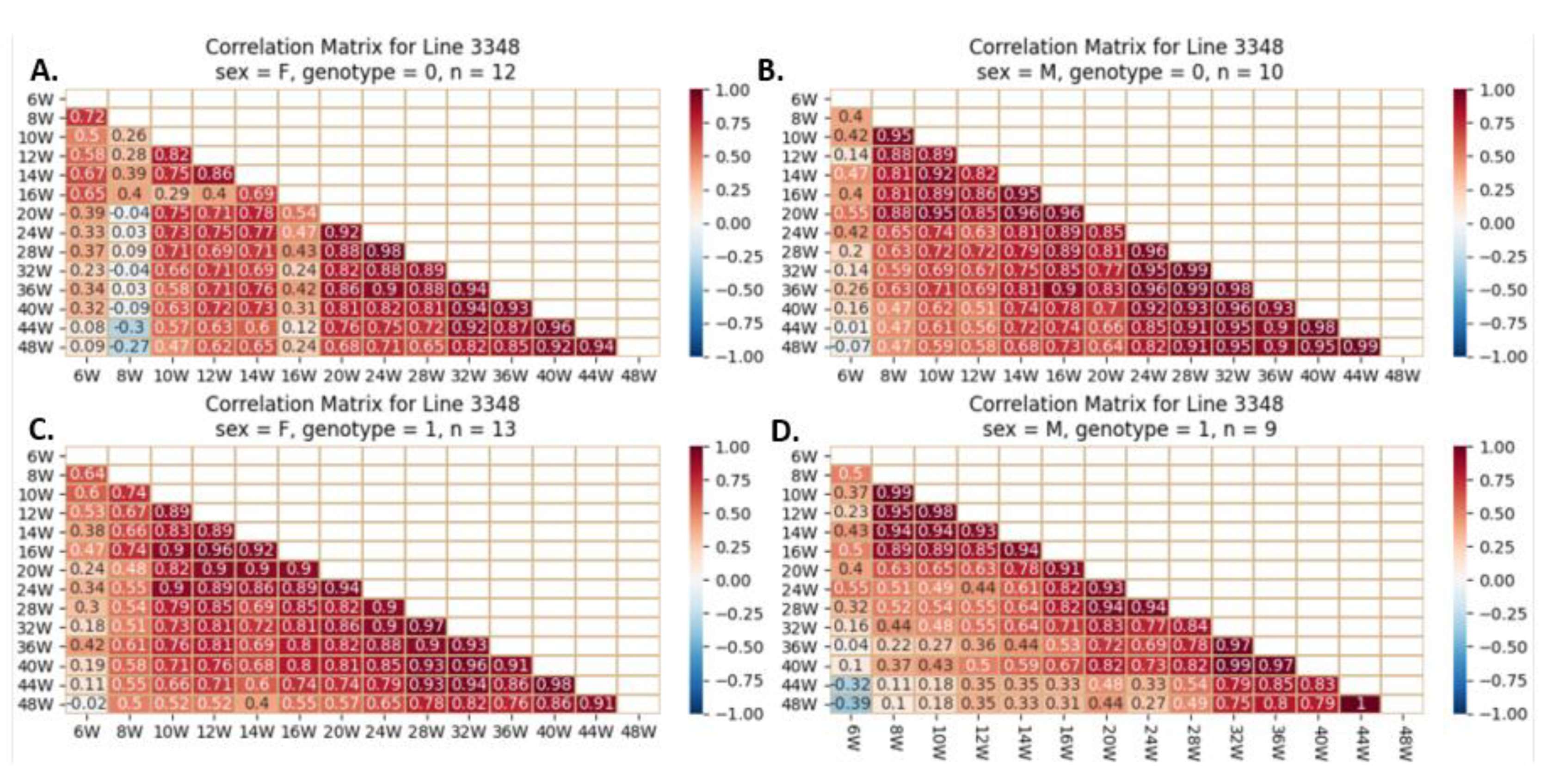
The heatmaps emphasize the differences between lines. There were different correlations between initial BW and final BW between lines and within lines regarding sex, and this is exacerbated in the presence of mutant tumor suppressors. Weight gain differs in populations with different genetic backgrounds as observed oreviously by Lone et al. [
44]. Some lines gained more weight in the presence of Smad4 knockout, while others gained less. It also depended on the gender of the mice, but in general, the presence of the mutation resulted in overweight mice. The finding that null alleles of mouse genes frequently reduce but occasionally increase BW is not unique [
45]. To our knowledge, no previous research has examined the overall effect of gene deletion on mice's BW because knockout studies are often done to answer specific gene research questions. However, Daniel et al. scanned the Mouse Genome Database for each knockout gene on six chromosomes to objectively analyze the effect of gene knockouts on BW [
46]. They estimate that more than 6,000 genes contribute to mouse body size, and 30% of null alleles result in a mouse with lower BW, while 3% result in a mouse with higher BW [
47]. The genome favors weight gain with ten times as many genes increasing size as decreasing. This supports the theory that mice are "hard-wired" to favor positive energy balance [
48].
In this research, we carried out a comparative analysis of various ML algorithms for predicting the genotype of mice. It was shown that ML algorithm Logistic Regression provided better results than common regression algorithms for prediction. A successful classification of a genotype based solely on weight has undeniable clinical utility. Although the cost of sequencing has decreased significantly over time, it is still not a common practice. Line IL6009 exhibited the highest level of predictability, with an AUC > 0.75 as predicted by four different models. As demonstrated by the correlation matrices, this line's behavior differed between the two genotypes. In line IL6012, for instance, the heatmaps are extremely similar, and the classification results are also lower. The results clearly show differences between lines. In other words, an individual's entire genotype influences the predictability of this Smad4 knockout gene. The interactions of this protein with other proteins within the cell could be a possible explanation for this phenomenon.
To predict the BW of mice, the global outcomes are anticipated; the more information we provide the algorithm, the more accurately it predicts. However, even when we only give the algorithm week 8, the results are quite good. The line-separated results are quite unexpected. While some lines, such as IL5008 and IL2513, are highly predictable from week 8 or even week 6, others, such as IL188, are entirely unpredictable. In addition, we observe that adding more data to the algorithm hinders its performance for some lines, including lines IL5000 and IL6009. The outcomes clearly vary between lines. We believe that these variations are due to the different genotypes of the lines, as the behavior varies based on genotype. Some behaviors are more predictable than others, particularly when a linear regression model is used. From what we have seen, for most lines it seems like there are 2 linear behaviors with a specific changing point slope-wise. In the future, it could be interesting to try to predict the time of change in the slope based on the initial features alone. Studies in mouse strains with various genetic backgrounds and established genetic structures provide unparalleled opportunities to find and analyze trait-related genomic loci. Additional lines with and without a mutation must be weighed for phenotype-genotype association analyses. Once acquired, such information can be used to forecast weight gain risk and build genetically based preventative and treatment techniques.
Overweight and obesity not just increase the risk of CVD and T2D, but also of many different types of cancers [
49]. Even though it is known that BW is a variable, efforts to stop the obesity epidemic have failed [
50]. The global burden of cancer has increased in tandem with the prevalence of obesity, and 13 types of cancer have been linked to fat [
51]. Breast (postmenopausal), colon–rectum, endometrium, ovary, pancreas, kidney, gallbladder, gastric cardia, liver, oesophagus (adenocarcinoma), meningioma, thyroid, and multiple myeloma are the cancers associated with overweight or obesity. However, there is a prominent research gap between weight gain and certain cancers linked to obesity. Consequently, there is a pressing need to monitor these mice and their weight at older ages and to determine if there is a correlation between the percentage of weight gain in mutant mice compared to the control group and cancer susceptibility of various types.
In the future, it would be interesting to use the advantages of Smad4 knockout CC mice to investigate additional phenotypes of MetS, such as insulin resistance, diabetes, and lipid metabolism, in addition to cancer susceptibility. Understanding how genetic background affects metabolic profiles in a Smad4 knockout setting is essential for precision medicine and individualized pharmaceutical therapies.
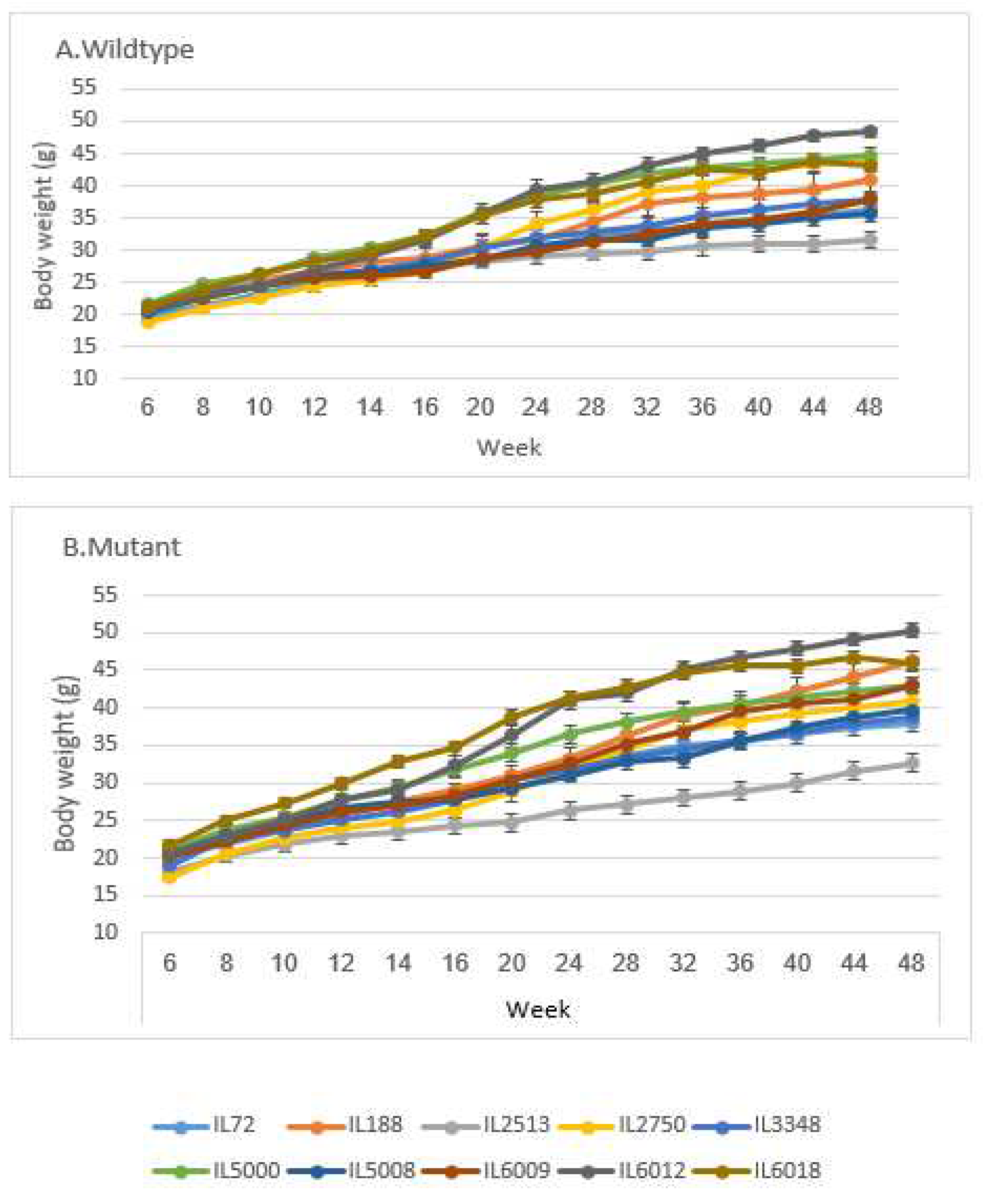
Figure 1.
BW (±SE) A of the control and B Smad4+/- groups at 14 time points (8, 10, 12, 14, 16, 20, 24, 28, 32, 36, 40, 44 and 48 weeks old) of 10 different sets of 10 different CC lines. The X-axis represents the time points (in weeks) while the Y-axis represents values of body weight (g). One-way ANOVA performed for statistical analysis, p < 0.05.
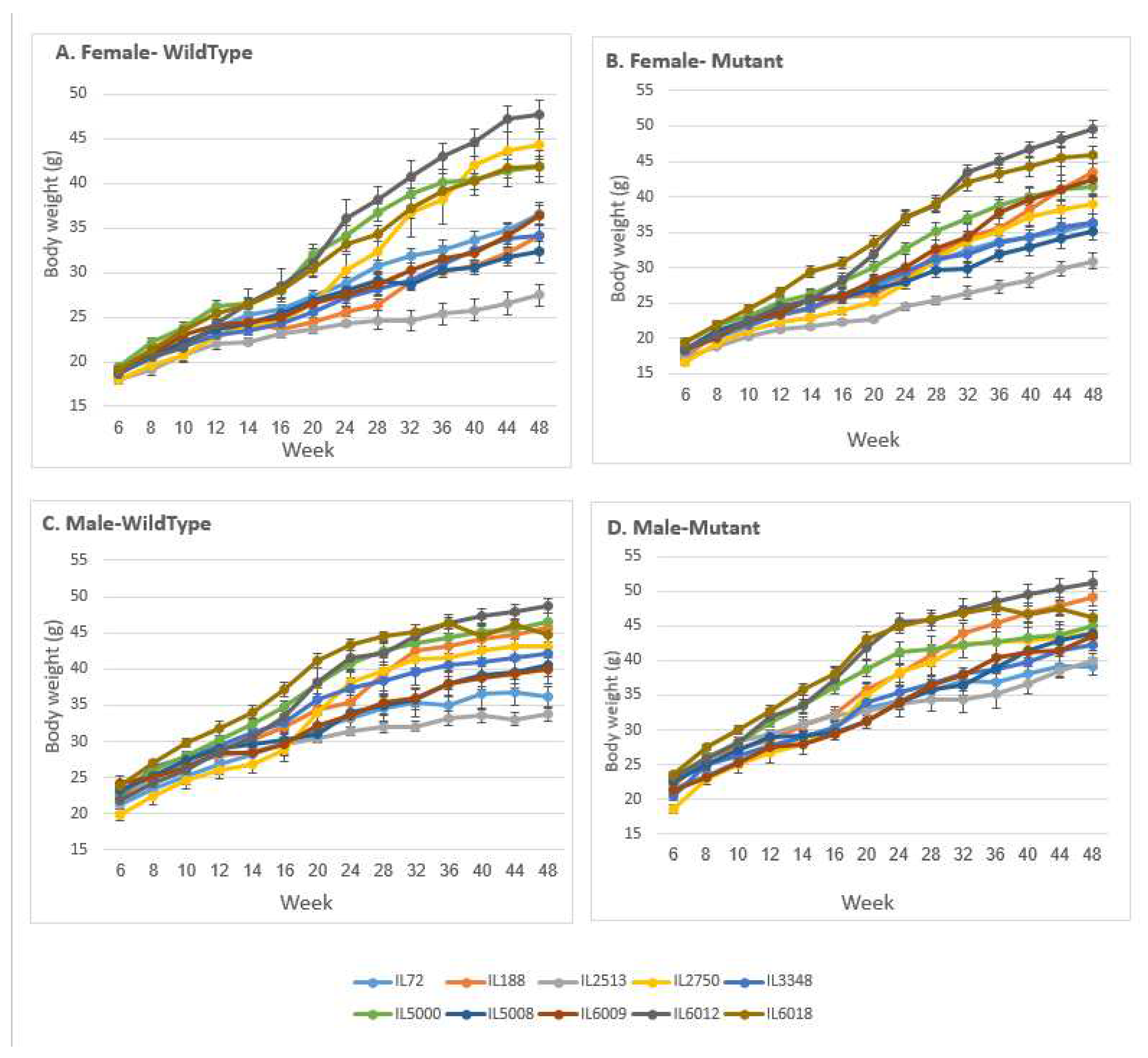
Figure 2.
Body weight (±SE) of the A, C control and B, D Smad4+/- groups at 14 time points (8, 10, 12, 14, 16, 20, 24, 28, 32, 36, 40, 44 and 48 weeks old) of 10 different set of CC lines. The X-axis represents the time points (in weeks) while the Y-axis represents values of body mass (g). One-way ANOVA performed for statistical analysis, p < 0.05.
Figure 3.
Body weight changes in wildtype and Smad4+/- mice at 14 time points for line IL2513 (6-48 weeks old). The X-axis depicts time points (in weeks), while the Y-axis depicts body weight values. The weight increase trend in this line is distinctive and distinct from the other lines; in the overall group, the weight of control mice is greater than the weight of mutant mice up to a reversal point at which the weight ratio reverses, which occurs at 44 weeks. The difference is significant between control mice and mutant mice BW from the start of the experiment to age of 20 weeks in overall group. In the female group, the bending point begins at 20-week-old reversal point and grows somewhat until the end of the experiment, but not significantly. There is no bending point in males. Mutant mice weighed more than control mice from the start of the experiment, but the difference in the weights grew with time and became significant only around week 44 and 48.
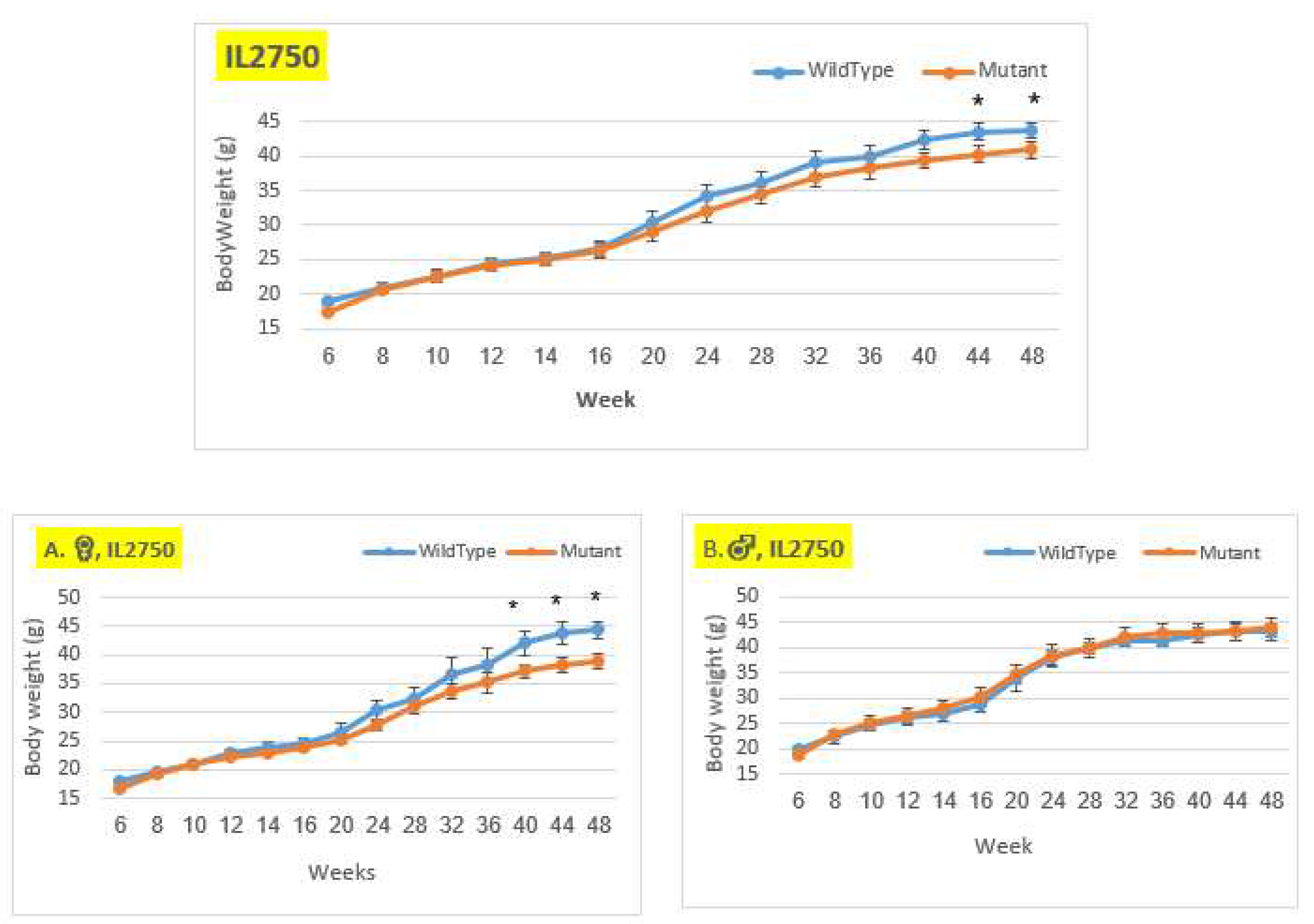
Figure 4.
Body weight changes in wildtype and Smad4+/- mice at 14 time points for line IL2750 (6-48 weeks old). The X-axis depicts time points (in weeks), while the Y-axis depicts body weight values. From week 20 through the end of the period, we may observe a difference in the weight of mutant mice compared to control mice in both the female and overall groups. Only from week 40 demonstrates a significant difference. There is no difference in the male group.
Figure 5.
Body weigh changes in wildtype and Smad4+/- mice at 14 time points for line IL5000 (6-48 weeks old). The X-axis depicts time points (in weeks), while the Y-axis depicts body weight values. Throughout the experiment, the control mice weighed more than the mutant mice, and the difference rose later in the experiment but did not achieve a statistically significant difference. A reversal points in the female group at week 24 where the mutant mice weighed more than the control mice and vice versa, but there was no significant difference. In the male group, control and mutant mice weighed the same from week 40 to week 48, whereas control mice weighed more before that. There was no discernible difference.
Figure 6.
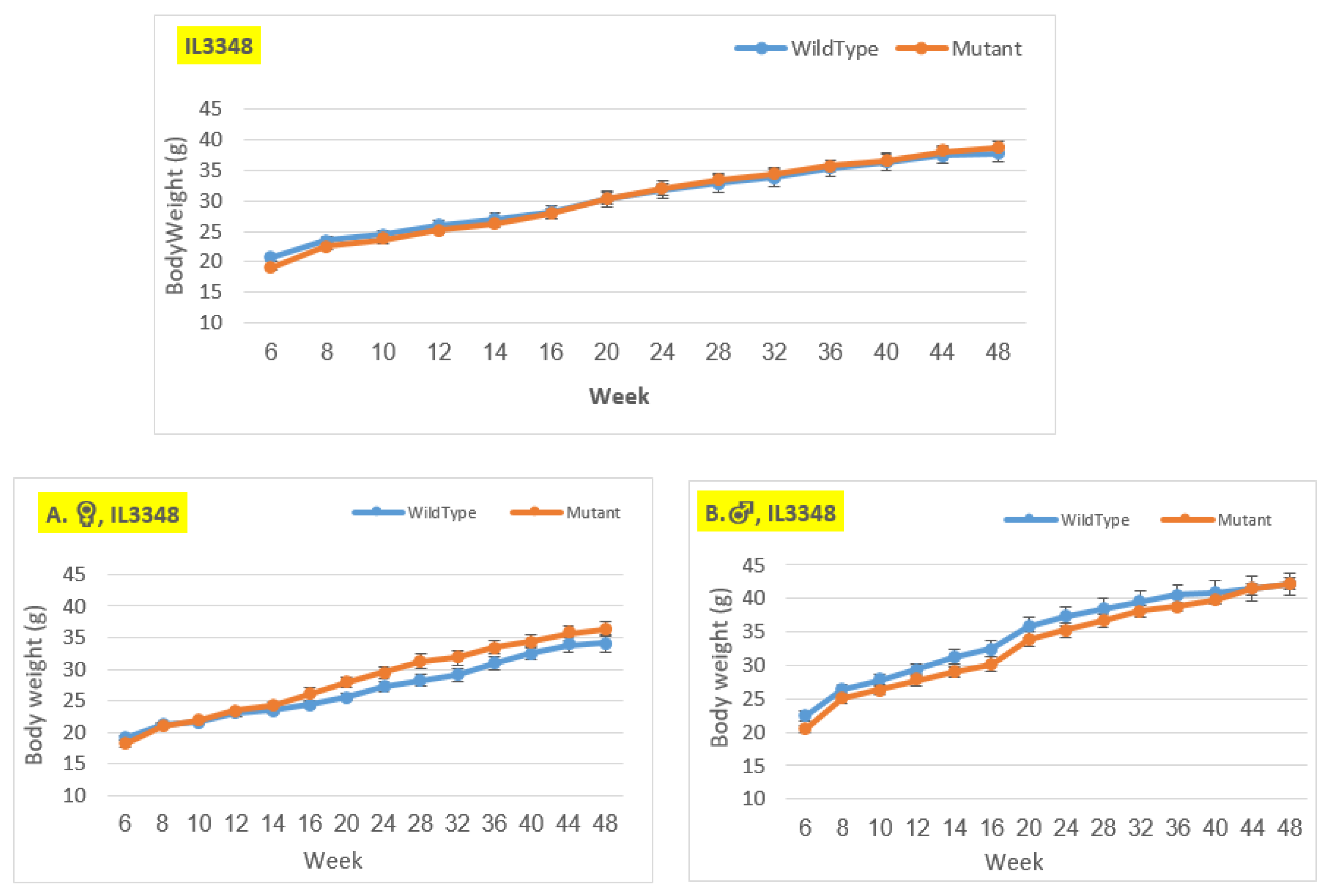
Body weight changes in wildtype and Smad4+/- mice at 14 time points for line IL3348 (6-48 weeks old). The X-axis depicts time points (in weeks), while the Y-axis depicts body weight values. The mutant mice weigh about the same as the control mice throughout the experiment in the overall group. Nonetheless, when analyzed by gender, in the female group, the mutant mice weighed more than the control mice from around week 14 to the end of the experiment, but the difference is not statistically significant. In contrast, in the male group, the control mice weighed more than the mutant mice from the beginning of the experiment until week 40, but there was no significant difference, and by weeks 44 and 48, their weight was nearly identical.
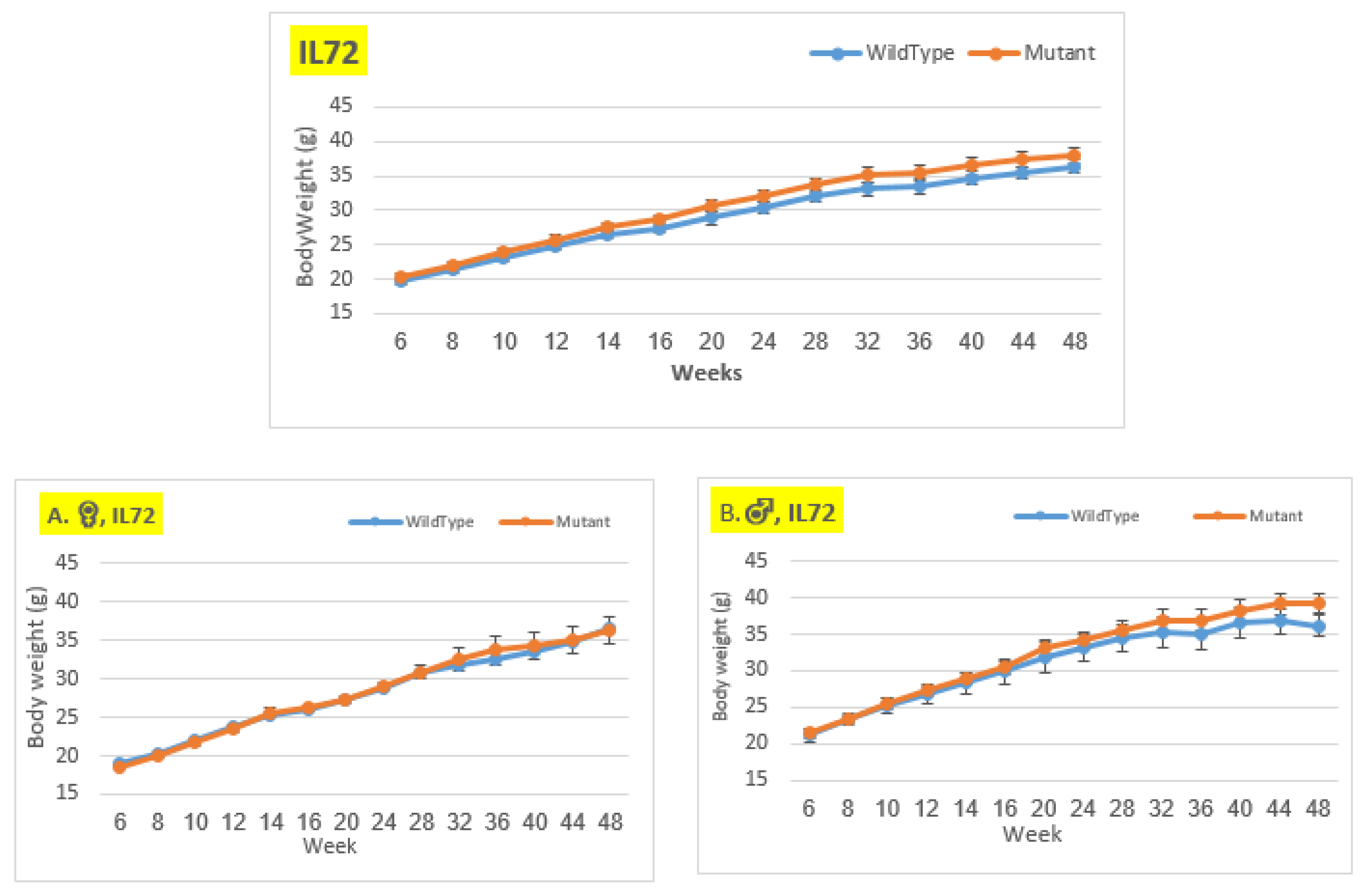
Figure 7.
Body weigh changes in wildtype and Smad4+/- mice at 14 time points for line IL72 (6-48 weeks old). The X-axis depicts time points (in weeks), while the Y-axis depicts body mass values in grams (g). We can see a difference in the weight of mice with a mutation compared to control mice in the male group from week 28 until the conclusion of the period, although it is not significant. In females and the overall group, there is essentially no difference in BW between mutant and wild type mice.
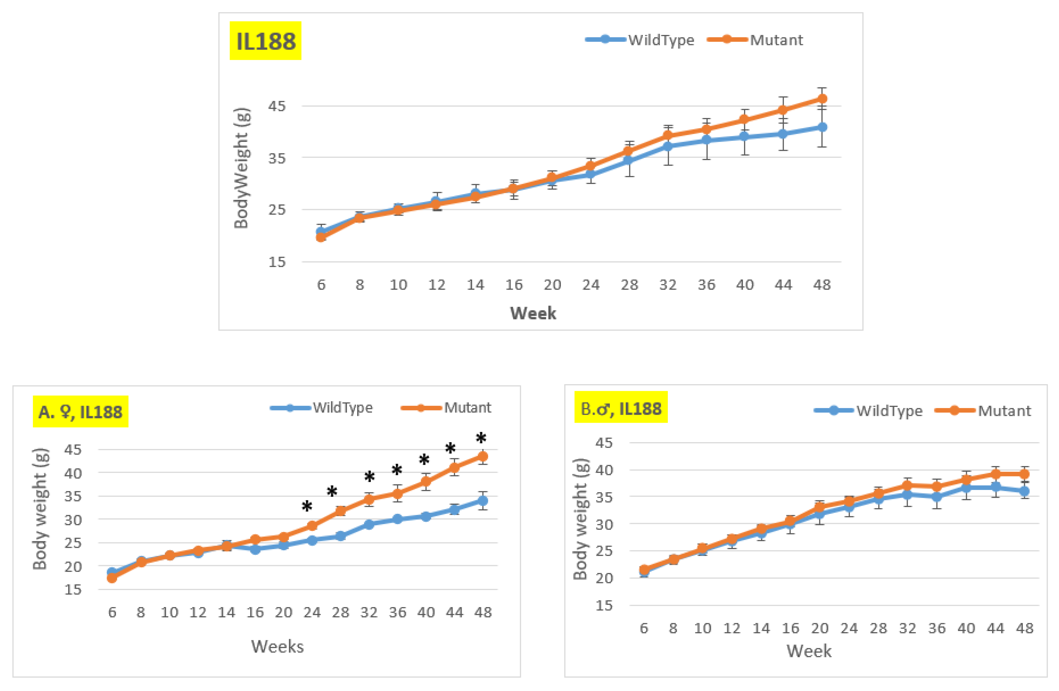
Figure 8.
Body weight changing of the wildtype and Smad4+/- mice for line IL188 at 14-time points (6-48 weeks old). The X-axis represents the time points (in weeks), while the Y-axis represents values of body mass. We can see a difference in the weight of mice with a mutation compared to control mice in all groups (males, females, and overall) from week 24 to the end of the period, although only the female group from week 24 shows a significant difference.
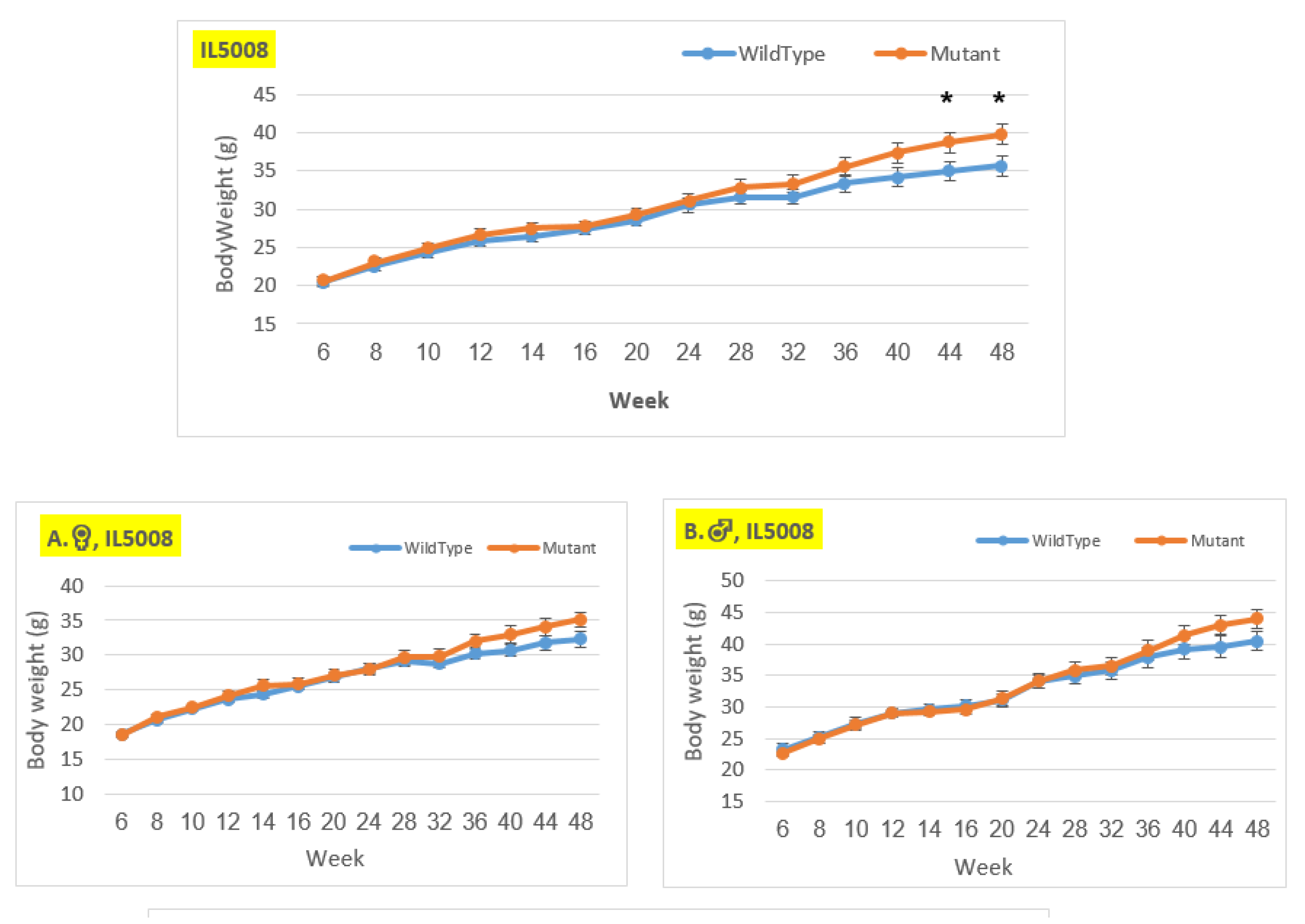
Figure 9.
Body weight changes in wildtype and Smad4+/- mice at 14 time points for line IL5008 (6-48 weeks old). The X-axis depicts time points (in weeks), while the Y-axis depicts body weight values. In this line, mutant mice weigh more than control mice in all three groups (males, females, and overall); however, the weight difference grew during the experiment and is only significant in the overall group at weeks 44 and 48.
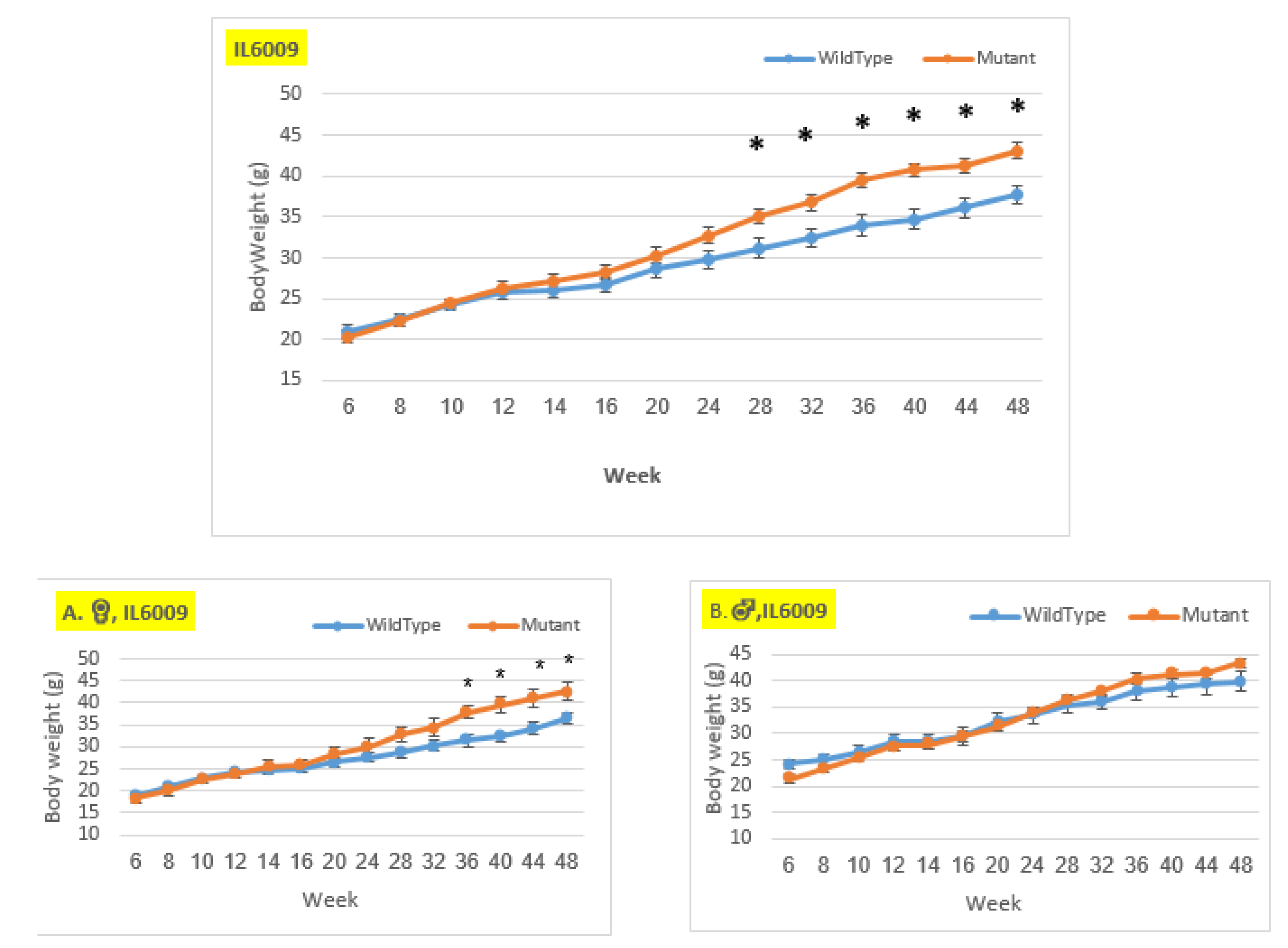
Figure 10.
Body weight changes in wildtype and Smad4+/- mice at 14 time points for line IL6009 (6-48 weeks old). The X-axis depicts time points (in weeks), while the Y-axis depicts body weight values. From week 14 through the end of the period, we may observe a difference in the weight of mutant mice compared to control mice in both the female and overall groups. Only from week 28 demonstrates a significant difference in the overall group and from week 36 a significant difference in the female group. In the male group, there is no significant change, until week 12, the control group weighed more than the mutant. Starting through the end of the experiment, the mutant mice weighed more than the control mice, but the difference was not significant.
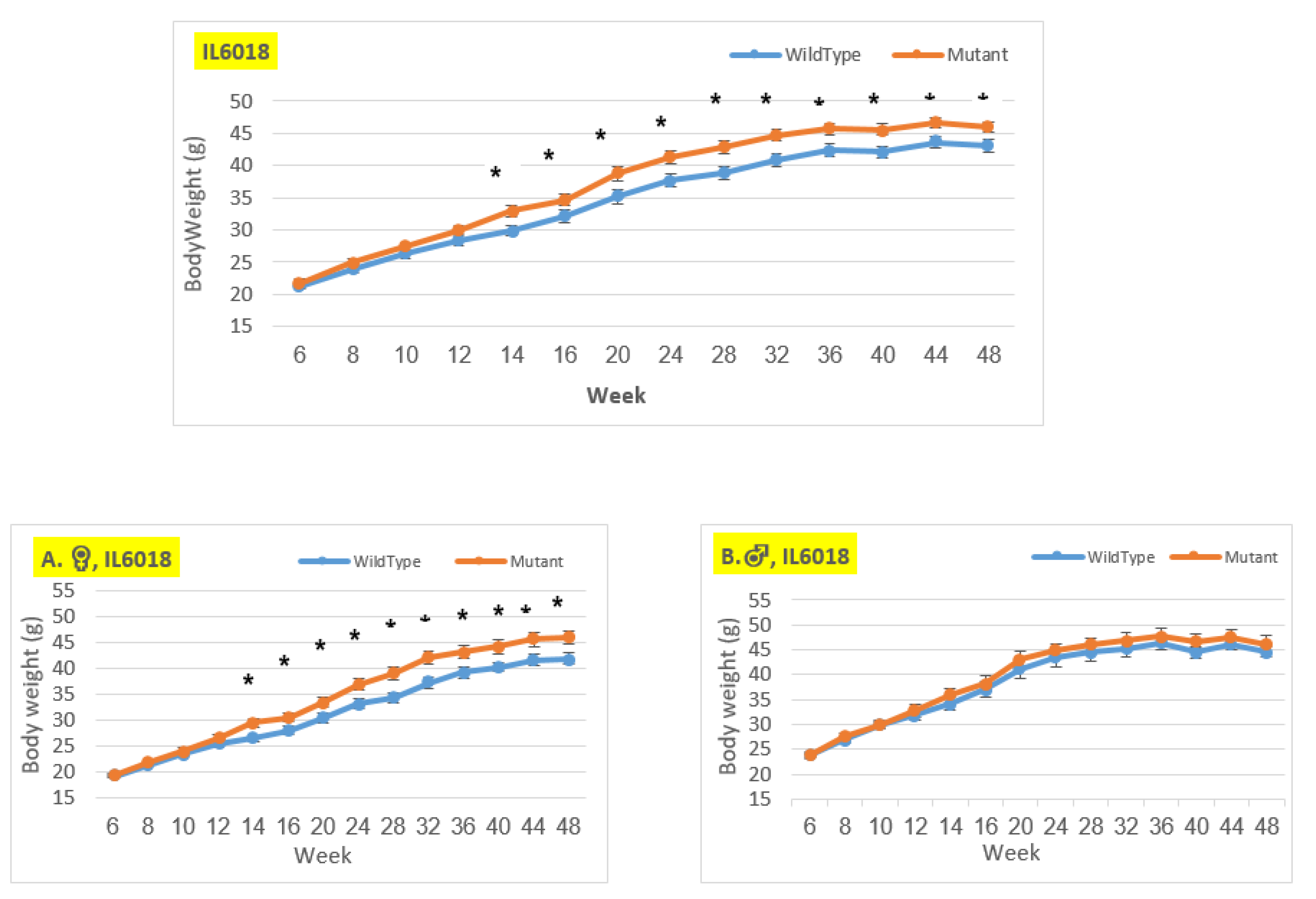
Figure 11.
Body weight changes in wildtype and Smad4+/- mice at 14 time points for line IL6018 (6-48 weeks old). The X-axis depicts time points (in weeks), while the Y-axis depicts body weight values. We may see a substantial difference in the weight of mutant mice compared to control mice in both the female and overall groups from week 14 to the end of the period. There is no difference between the male groups.
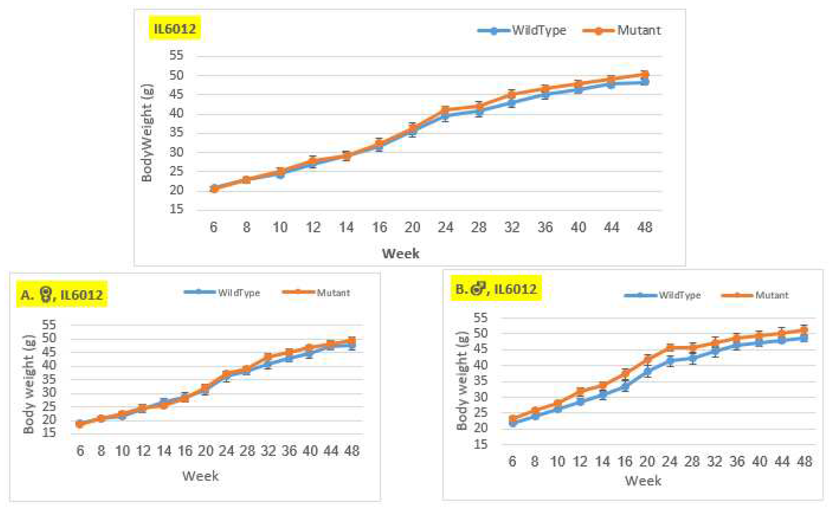
Figure 12.
Body weigh changes in wildtype and Smad4+/- mice at 14 time points for line IL6012 (6-48 weeks old). The X-axis depicts time points (in weeks), while the Y-axis depicts body weight values. In the overall group and the female group, the weight of the mutant mice was practically identical to that of the control mice from the beginning of the experiment until about week 20, after which the mutation mice weighed more than the control mice until the end of the experiment. In the male group, mutant mice consistently weighed more than control mice throughout the duration of the experiment, without any significant difference.
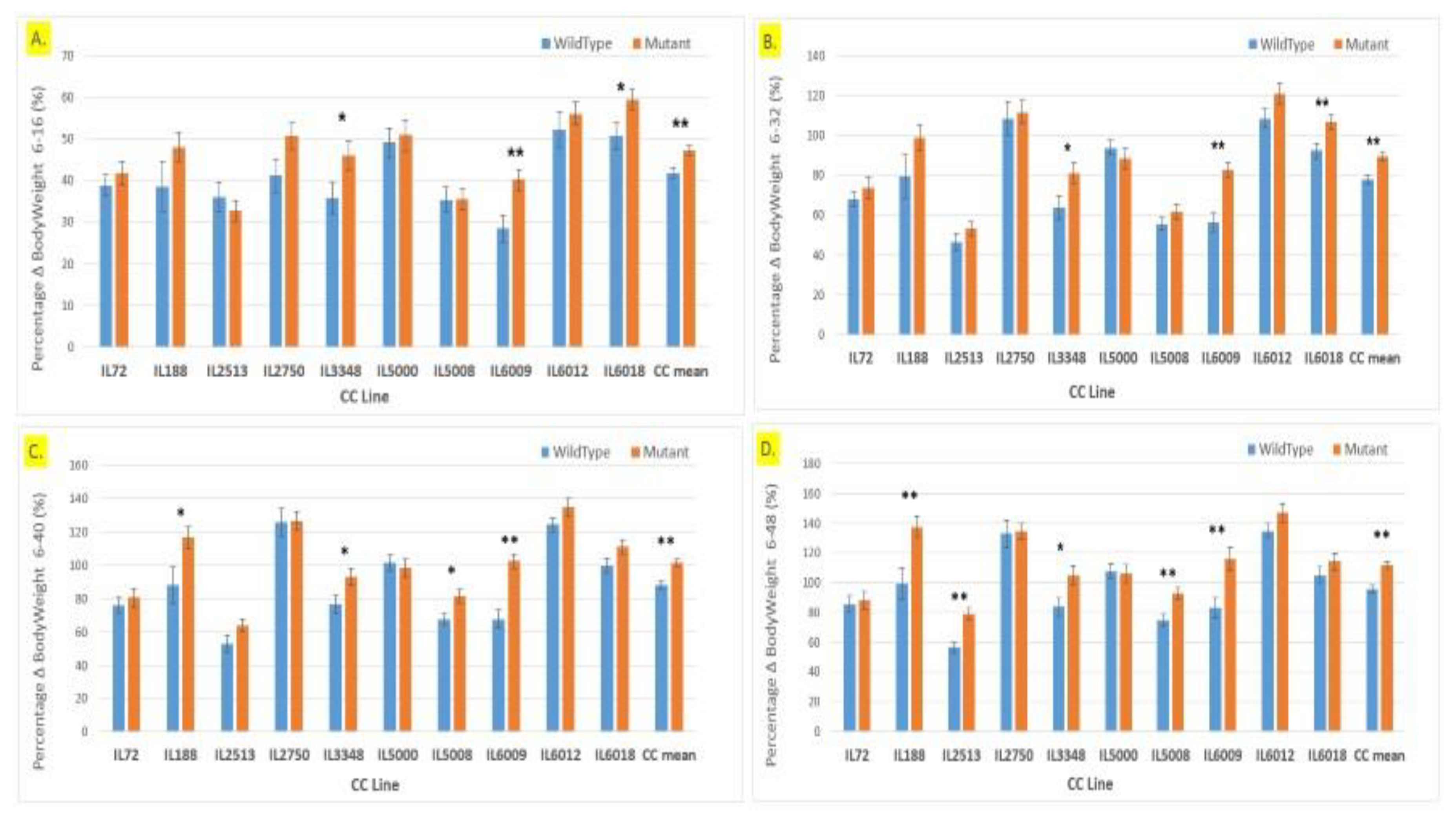
Figure 13.
Percentage body weight gain (g) of ten different CC lines after 48 weeks of BW monitoring in the overall F1 population (males and females). (A) Shows BW percentage gain in 10 different lines of F1 population with mutation vs. wild type until week 16, BW percentage gain until week 32 is shown in (B), (C) Shows the percentage increase in BW until week 40, and (D) the percentage increase in BW until week 48.
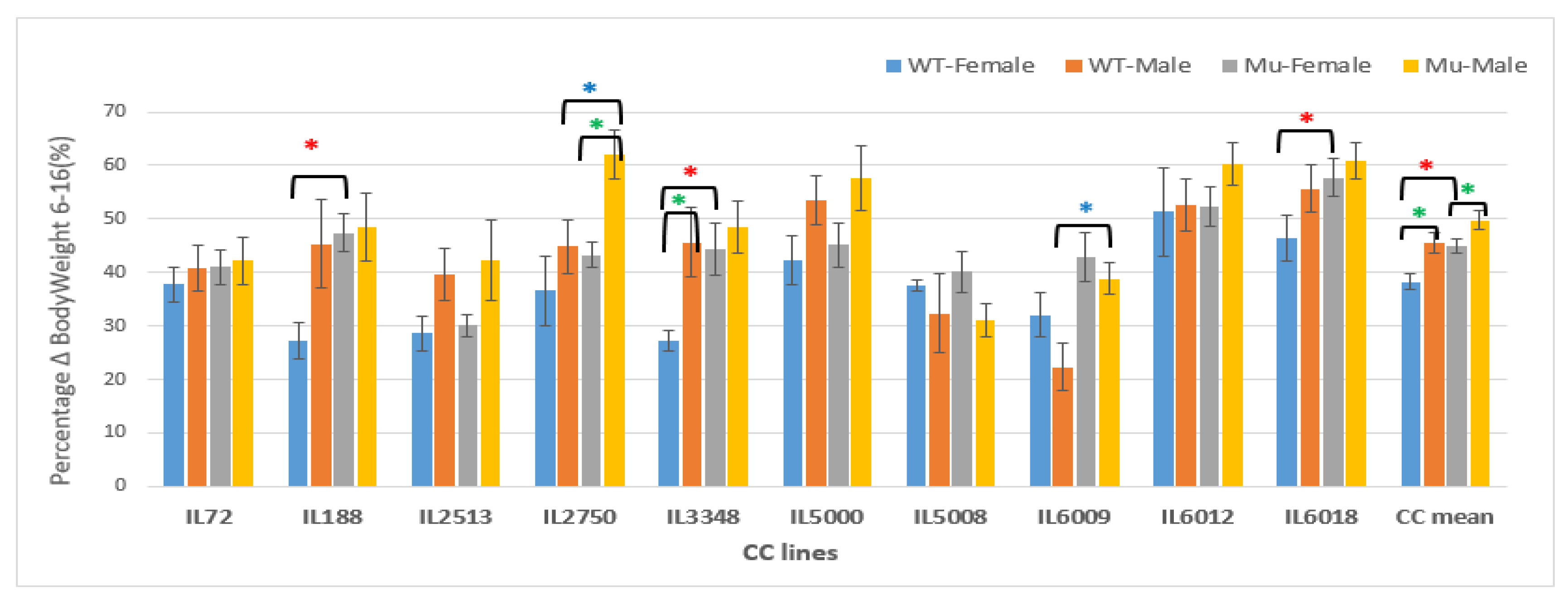
Figure 14.
Percentage changes in Body weight in grams (g) between weeks 6-16 of ten CC lines, separately for females and males, having wildtype and mutant genotypes. The X-axis depicts the various CC lines, while the Y-axis depicts the percentage change in BW over weeks 6-16.
Figure 14.
Percentage changes in Body weight in grams (g) between weeks 6-16 of ten CC lines, separately for females and males, having wildtype and mutant genotypes. The X-axis depicts the various CC lines, while the Y-axis depicts the percentage change in BW over weeks 6-16.
Figure 15.
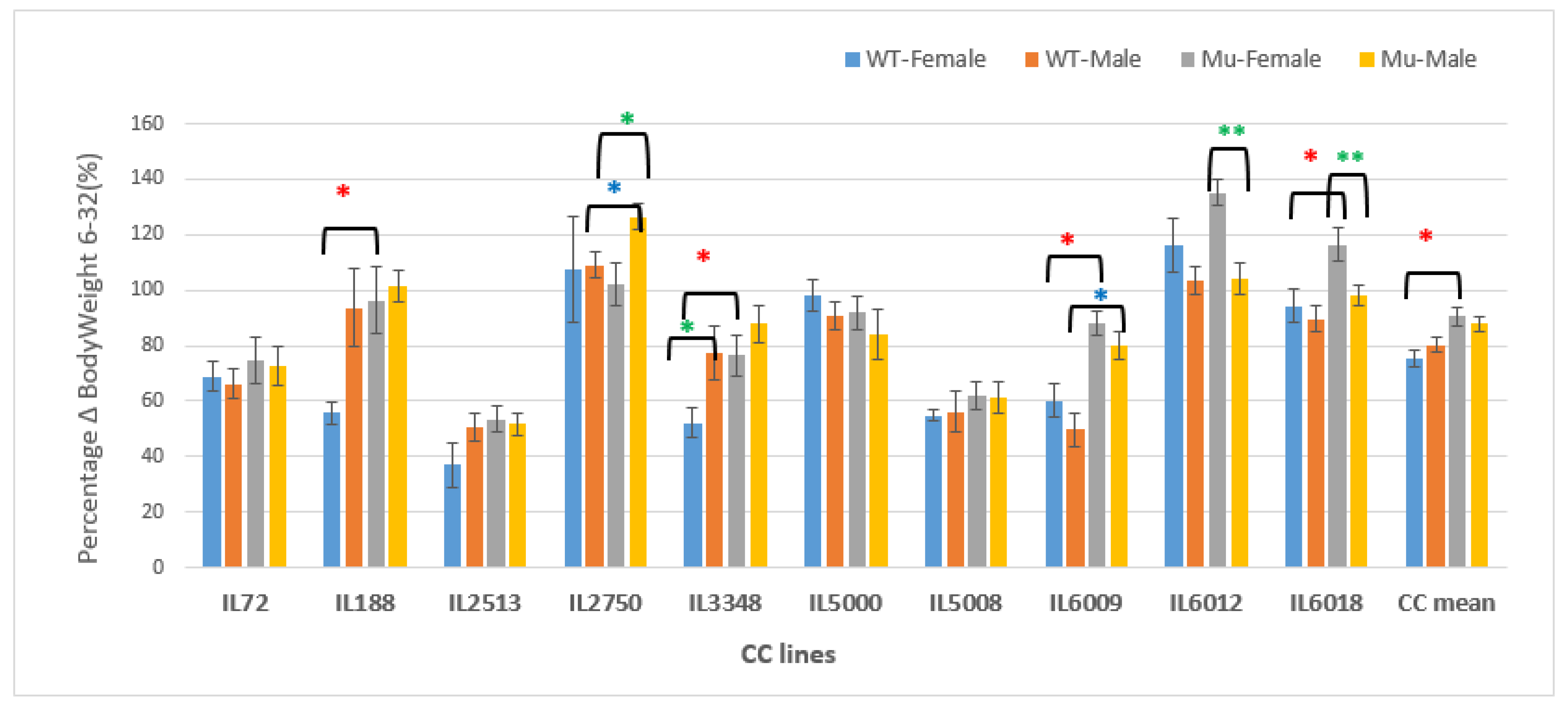
Percentage changes in body weight in grams (g) between weeks 6-32 of ten CC lines, separately for females and males, having wildtype and mutant genotypes. The X-axis depicts the various CC lines, while the Y-axis depicts the percentage change in BW over weeks 6-32.
Figure 15.
Percentage changes in body weight in grams (g) between weeks 6-32 of ten CC lines, separately for females and males, having wildtype and mutant genotypes. The X-axis depicts the various CC lines, while the Y-axis depicts the percentage change in BW over weeks 6-32.
Figure 16.
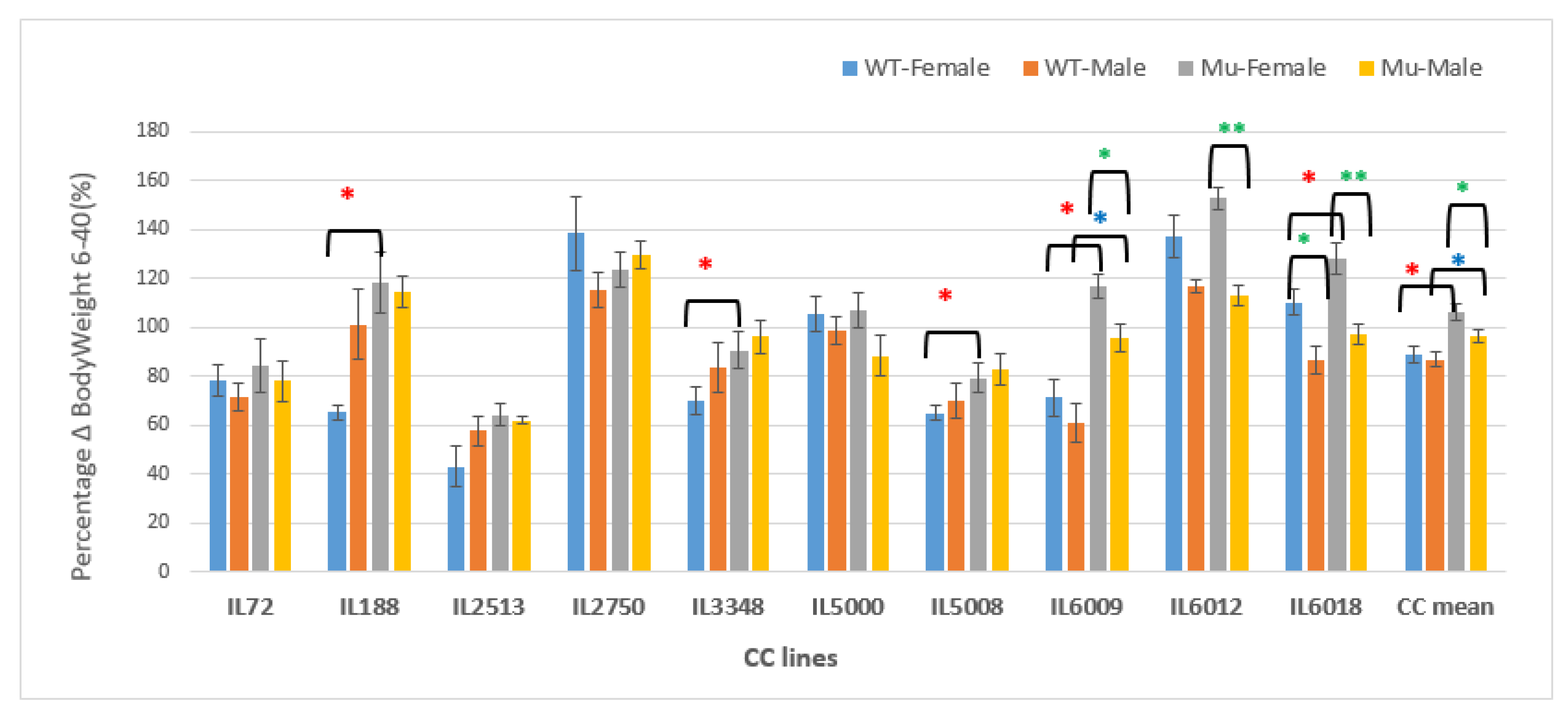
Changes in BW as a percentage in grams (g) between weeks 6-40 of ten CC lines, separately for females and males, having wildtype and mutant genotypes. The X-axis depicts the various CC lines, while the Y-axis depicts the percentage change in BW over weeks 6-40.
Figure 16.
Changes in BW as a percentage in grams (g) between weeks 6-40 of ten CC lines, separately for females and males, having wildtype and mutant genotypes. The X-axis depicts the various CC lines, while the Y-axis depicts the percentage change in BW over weeks 6-40.
Figure 17.
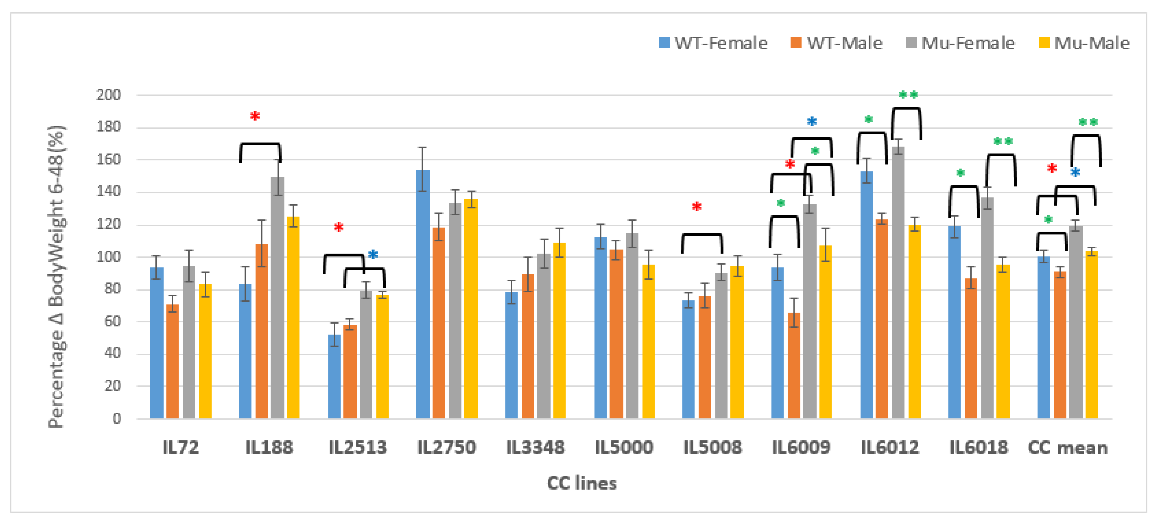
Changes in BW as a percentage in grams (g) between weeks 6-48 of ten CC lines, separately for females and males, having wildtype and mutant genotypes. The X-axis depicts the various CC lines, while the Y-axis depicts the percentage change in BW over weeks 6-48.
Figure 17.
Changes in BW as a percentage in grams (g) between weeks 6-48 of ten CC lines, separately for females and males, having wildtype and mutant genotypes. The X-axis depicts the various CC lines, while the Y-axis depicts the percentage change in BW over weeks 6-48.
Figure 18.
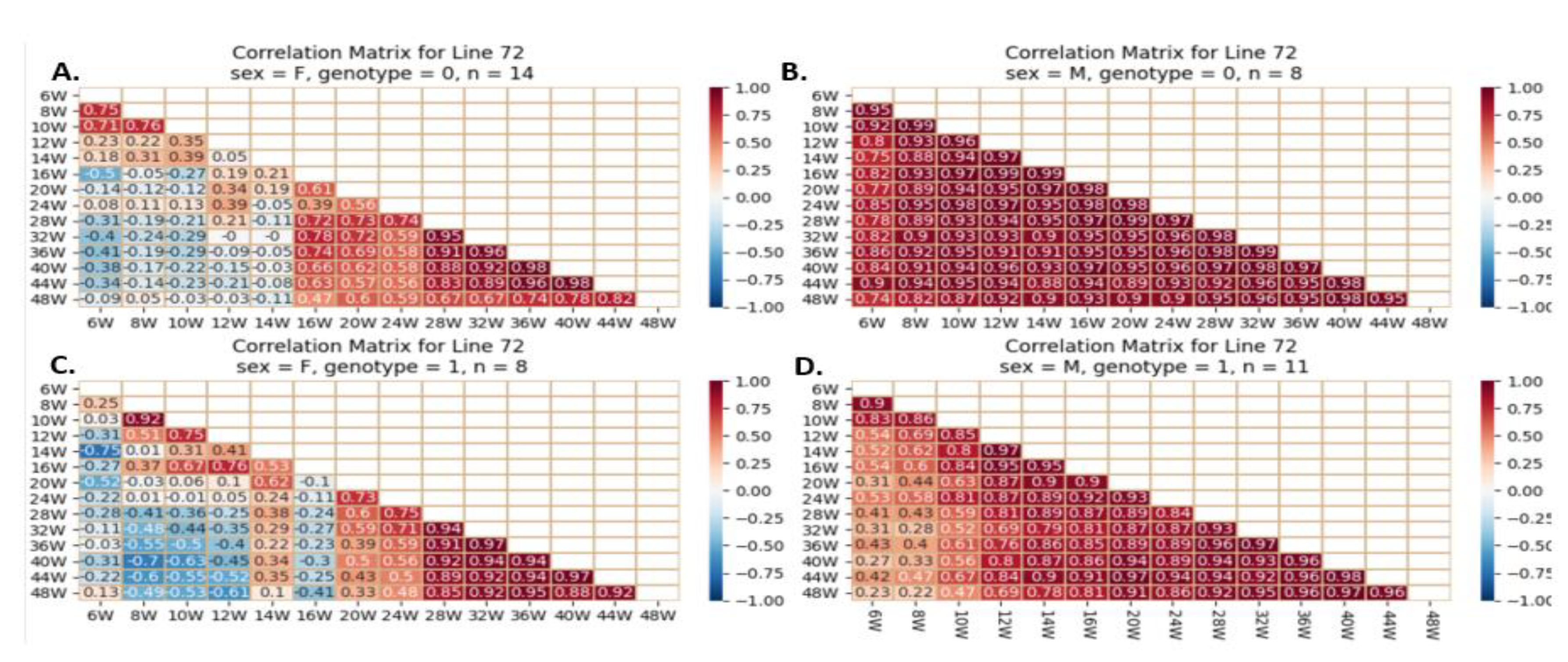
Heatmap and Pearson correlation between the body weight of female and male mice of line IL72, either wild-type or mutant, between various weeks. Figures (A) depict wildtype female, (B) wildtype male, (C) mutant female, and (D) mutant male. The r values ranged from minimum (-1) to maximum (1).
Figure 19.
Heatmap and Pearson correlation between the body weight of female and male mice of line IL3348, either wild-type or mutant, between various weeks. Figures (A) depict wildtype female, (B) wildtype male, (C) mutant female, and (D) mutant male. The r values ranged from minimum (-1) to maximum (1).
Figure 20.
Heatmap and Pearson correlation between the body weight of female and male mice of line IL6009, either wild-type or mutant, between various weeks. Figures (A) depict wildtype female, (B) wildtype male, (C) mutant female, and (D) mutant male. The r values ranged from minimum (-1) to maximum (1).
Table 1.
Summary table of the total number (N) of F1 mice from each CC line males and females separately assessed in each study group (Wildtype VS Mutant).
Table 1.
Summary table of the total number (N) of F1 mice from each CC line males and females separately assessed in each study group (Wildtype VS Mutant).
| |
Male |
Female |
|
| |
wild type |
Mutant |
Wild type |
Mutant |
|
| IL72 |
8 |
11 |
14 |
8 |
41 |
| IL188 |
5 |
8 |
3 |
8 |
24 |
| IL2513 |
8 |
3 |
4 |
12 |
27 |
| IL2750 |
6 |
7 |
6 |
11 |
30 |
| IL3348 |
10 |
9 |
12 |
13 |
44 |
| IL5000 |
14 |
10 |
9 |
12 |
45 |
| IL5008 |
9 |
12 |
13 |
11 |
45 |
| IL6009 |
6 |
10 |
10 |
5 |
31 |
| IL6012 |
10 |
9 |
6 |
11 |
36 |
| IL6018 |
16 |
18 |
19 |
15 |
69 |
| |
|
|
|
Total |
391 |
Table 2.
Comparing the prevalence of wild-type mice to mutant mice in the SMAD4 gene and the predominance of female mice to that of male mice.
Table 2.
Comparing the prevalence of wild-type mice to mutant mice in the SMAD4 gene and the predominance of female mice to that of male mice.
| |
Frequency |
Percent (%) |
Total |
| Wild Type |
188 |
48.1 |
|
| Mutant |
203 |
51.9 |
|
| Female |
202 |
51.7 |
|
| Male |
189 |
48.3 |
|
| |
|
|
391 (100%) |
Table 3.
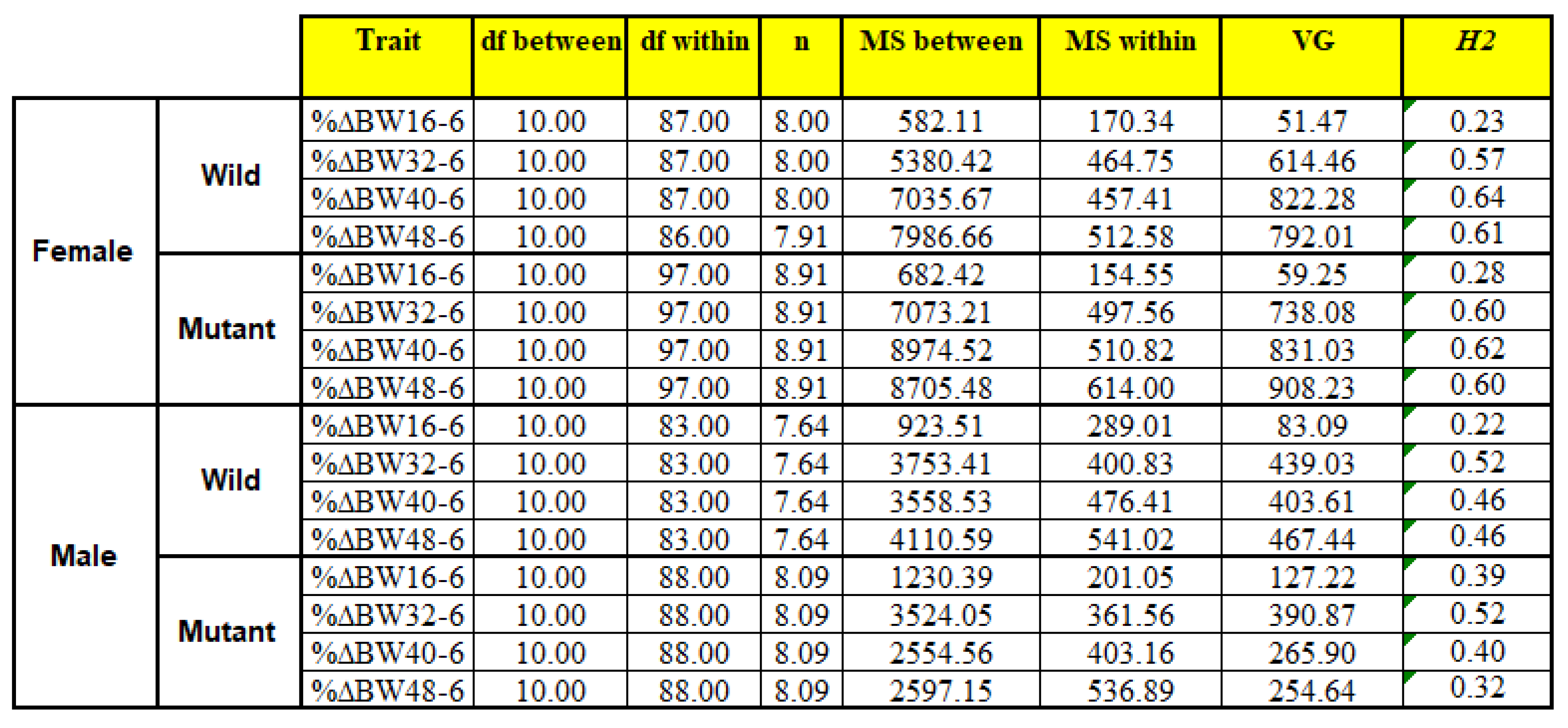
Exhibit the results of calculating heritability (H2) values. The heritability was calculated using One-Way ANOVA for%BW6-16, %BW6-32, %BW6-40, %BW6-48 traits that were calculated separately by sex and genotype.
Table 3.
Exhibit the results of calculating heritability (H2) values. The heritability was calculated using One-Way ANOVA for%BW6-16, %BW6-32, %BW6-40, %BW6-48 traits that were calculated separately by sex and genotype.
Table 4.
Displays the results of six different classification algorithms for each line to predict the genotype (0/1) of a mouse based on its sex and 14 recorded weights.
Table 4.
Displays the results of six different classification algorithms for each line to predict the genotype (0/1) of a mouse based on its sex and 14 recorded weights.
| Line |
IL72 |
IL188 |
IL2513 |
IL2750 |
IL3348 |
IL5000 |
IL5008 |
IL6009 |
IL6012 |
IL6018 |
| N |
41 |
24 |
27 |
29 |
44 |
45 |
45 |
31 |
36 |
69 |
| 6W |
0.29 |
-0.30 |
0.64 |
0.08 |
0.30 |
0.35 |
0.38 |
0.23 |
0.33 |
0.44 |
| 8W |
0.24 |
-0.21 |
0.63 |
0.13 |
0.37 |
0.37 |
0.56 |
0.15 |
0.27 |
0.53 |
| 10W |
0.26 |
-0.03 |
0.60 |
0.28 |
0.57 |
0.39 |
0.53 |
0.08 |
0.37 |
0.51 |
| 12W |
0.35 |
-0.20 |
0.64 |
0.44 |
0.52 |
0.32 |
0.52 |
0.13 |
0.27 |
0.48 |
| 14W |
0.43 |
-0.32 |
0.59 |
0.41 |
0.54 |
0.25 |
0.54 |
0.03 |
0.32 |
0.61 |
| 16W |
0.32 |
-0.40 |
0.56 |
0.33 |
0.53 |
0.21 |
0.58 |
-0.15 |
0.31 |
0.64 |
| 20W |
0.47 |
-1.23 |
0.42 |
0.13 |
0.51 |
0.20 |
0.71 |
-0.12 |
0.25 |
0.61 |
| 24W |
0.46 |
-1.58 |
0.55 |
0.15 |
0.66 |
0.06 |
0.74 |
-0.28 |
0.40 |
0.61 |
Table 5.
Displays the results of BW prediction algorithms for each line to predict the genotype (0/1) of a mouse based on its sex and 14 recorded weights.
Table 5.
Displays the results of BW prediction algorithms for each line to predict the genotype (0/1) of a mouse based on its sex and 14 recorded weights.
| Line |
IL72 |
IL188 |
IL2513 |
IL2750 |
IL3348 |
IL5000 |
IL5008 |
IL6009 |
IL6012 |
IL6018 |
| N |
41 |
24 |
27 |
29 |
44 |
45 |
45 |
31 |
36 |
69 |
| DT |
0.504 |
0.5 |
0.652 |
0.513 |
0.41 |
0.497 |
0.543 |
0.58 |
0.494 |
0.433 |
| NaBa |
0.603 |
0.459 |
0.67 |
0.58 |
0.553 |
0.491 |
0.584 |
0.798 |
0.528 |
0.644 |
| KNN |
0.506 |
0.5 |
0.718 |
0.637 |
0.555 |
0.42 |
0.556 |
0.787 |
0.483 |
0.539 |
| RF |
0.543 |
0.619 |
0.747 |
0.546 |
0.571 |
0.512 |
0.457 |
0.718 |
0.518 |
0.561 |
| SVC |
0.418 |
0.438 |
0.682 |
0.386 |
0.407 |
0.472 |
0.325 |
0.836 |
0.459 |
0.576 |
| LR |
0.332 |
0.747 |
0.875 |
0.752 |
0.531 |
0.392 |
0.557 |
0.82 |
0.405 |
0.586 |
