1. Introduction
Deep learning is a subset of machine learning that has exploded in popularity and become prominent in many industries around the world today because it is based on powerful artificial neural networks that are capable of learning and performing complex tasks such as Natural Language Processing [
1] and Image Classification [
2]. As a result, deep learning has also become useful and ubiquitous for remote sensing tasks because it has the computational power to extract compact features from data with high spectral and spatial resolution used for purposes such as object detection, land use and landscape classification [
3,
4,
5], and multi-class classification [
6,
7,
8]. Based on the successful performance of parallel text processing, Transformers [
9] have gained significant momentum in the deep learning domain. Transformer neural networks are models that are highly adept at learning context from input data using parallel multi-head attention mechanisms [
10]. As a result, they can be applied to remote sensing tasks such as multi-class classification of images because transformers can extract long-range dependencies from the relationships between elements of an image sequence to generate global representations.
Although Transformers can be applied for image analysis, CNNs are generally the dominant model for most aspects of computer vision. CNN models are typically more compact and resource-efficient while Transformers are usually large, requiring significant Graphics Processing Units (GPUs) for training. However, Transformers are able to get contextual understanding and global dependencies from images using self-attention unlike CNNs which typically use local operations that are restricted to small parts of images. This research demonstrates that a combination of CNNs and Transformers can be optimized to extract both local and global contextual information for image classification. To achieve this objective, we propose modifications in the Mobile Vision Transformer (ViT) [
11] model as it closely relates a blend of CNN and Vision Transformers. Our findings demonstrate a higher classification performance can be achieved even by using lightweight convolutional variants only if they are used strategically in the entire architecture. Motivated by our previous work on ShuffleNet optimization [
12], this research further solidifies our approach to build lightweight deep learning models without reducing accuracy.
In summary, here are our main contributions in this paper:
All model variants reduce the original MobileViT’s training parameters by replacing expensive CNN modules with a combination of Average Pooling, Depthwise Separable Convolution, and ShuffleNet blocks. Our models retain the benefits of CNN and Transformers and use them to boost performance on geospatial datasets without some of the other unnecessary costs.
The usage of convolution layers combined with the self-attention layers of Transformers inside the Mobile ViT variants provides better performance across all geospatial datasets when compared with the standalone ViT model that uses 95% more parameters than the Mobile ViT variants.
We test our proposed architectures on 4 geospatial datasets generating 80 models and conform to testing standards as presented in literature. The trained models are also made available on GitHub (
Link) for benchmarking and research purposes.
2. Previous Work
Vision transformers (ViTs) and Transformer architectures have already been applied in the remote sensing domain for tasks such as classifying various types of high-resolution UAV images. For example, the researchers of the AiTLAS Benchmark Arena train ViT and nine other representative architectures that are either CNN or Transformer-based on various multi-class classification datasets [
13]. In addition, some of the models are trained from scratch while others are pre-trained using ImageNet-1K weights. Then, multiple models of each representative type and pre-training status are generated to create more than 500 models that are then evaluated on their respective datasets before having their accuracies averaged to get the final result. Authors in [
14] utilize ViTs and their self-attention mechanism to achieve extremely accurate results when attempting to classify images of various crops and plant life. ViTs architecture allows it to focus on specific parts by enhancing or weakening predicted pixels within a feature map while ignoring the other perceptible aspects. However, these works simply don’t address the MobileViT model which combines CNNs and Transformers. As a result experiments don’t support how computationally expensive CNN layers are and if modifying them would provide a better outcome. Another application of ViT for remote sensing image classification was demonstrated in [
15] where compressed ViT models with a reduced number of redundant encoder layers was created before being trained on geospatial datasets. The results showed that using encoders with at least five layers yield accuracy of over 90% and adding more encoder layers after that only leads to 2% increases in accuracy. Another work that utilizes only parts of the ViT model instead of the entire architecture is demonstrated in [
16] which combines Channel-Spatial Attention (CSA) and the Multi-Head Self-Attention (MHSA) in ViTs to create an effective high-resolution remote sensing (HRRS) image scene classification network called Channel-Spatial Attention Transformer (CSAT). The ViT’s MHSA mechanism is extremely useful for this work and boosts the overall model’s performance on geospatial datasets because it can extract global features and learn long-range dependencies which helps encode the patches with global contextual information. While works that modify ViTs in order to reduce the number of parameters but retaining its benefits are useful, researchers were unable to combine the benefits of CNNs with MobileViT to achieve a desired outcome.
MobileViT has been applied for various purposes in fields where computer science is heavily applied as demonstrated in [
17]. In this research, authors create a drone detection algorithm that has a lightweight MobileViTv1 backbone feature extractor and multi-scale attention feature fusion network (CA-PANet). The backbone allows the algorithm to fully extract local and global features due to its combined CNN and Transformer architecture which helps the network extract target location information with high accuracy and a lesser number of parameters relative to other methods. Another application was outlined in [
18] which creates an automatic Diabetic Retinopathy (DR) grading framework that has a ResNet101 (CNN) backbone and custom MobileViT-Plus backbone to extract local and global information that will be fused together to assign DR grades (none, mild, moderate, severe) for 2D fundus images. The custom MobileViT-Plus backbone was made during the research and is made using depthwise separable convolutions as well as MobileViT-Plus blocks which replaces the Transformer block with a lightweight-Transformer block. As a result, the model is able to obtain results quickly with lower costs relative to ViT models while achieving better results when compared to MobileViT and other models such as Resnext101 [
19] and Se_resnet101 [
20].
Although work applying the relatively lightweight but powerful MobileViT to a different fields such as drones and healthcare is important, this research highlight fusion of ResNets with MobileNets which increases model complexity. ResNets are to some extent costlier replacements to options like pooling, MobileNet [
21] and ShuffleNet [
22]. Additionally, the model was trained to predict only five classes compared to the extensive number of land-cover classes in geospatial datasets with textual variation. A prior work that attempted to modify MobileViT models to boost performance was also reported in [
23] which replaces a 3 × 3 convolution layer in the Fusion block with a 1 × 1 convolution layer and replaces a 3 × 3 convolution layer in the Global Representation block with a depthwise convolution layer. Also, the model fuses the input features, combines Local and Global features, and increases the number of channels of the layers. Moreover, the model called MobileViTv3 is able to outperform MobileViT variants such as MobileVitv1-XS and MobileViTv2-0.75 while maintaining a similar but slightly higher number of parameters. Another attempt to modify MobileViT for better performance and lower latency is demonstrated in [
24] which replaces the MHSA in the MobileViTv1_Block’s Transformer Block with a separable self-attention method and does not use MobileViTv1_Block’s skip-connection and Fusion Block. As a result, MobileViTv2 maintains a similar or smaller number of parameters and outperforms the MobileViTv1 model by about 0.9% on the ImageNet dataset. While these works are able to modify MobileViTs in a way that minimizes costs and boosts performance, the number of parameters used is still to high at around more than 1.25 million (MobileViTv3-XXS), and the increase in accuracy (0.9% by MobileViTv2) from the original MobileViT architecture is negligible. This is a big drawback to implementing plug-and-play AI models in real world with resources-constrained environments.
3. Materials and Methods
3.1. Vision Transformers
Vision Transformers [
25] splits an image into patches before flattening those patches and converting them into linear embeddings with positional embeddings added to them. The sequence is then fed into a standard transformer encoder which consists of alternating Multi-Head Self Attention (MHSA) layers that map the input sequence to linear embeddings which are decoded to produce the logits. This model’s architecture can be seen in
Figure 1. Since ViT models deal with image patches at a global level using the self-attention mechanism, they can attain high levels of performance because they can capture contextual information and long-range dependencies between image pixels. However, there are many significant drawbacks of ViT such as the exorbitant amount of training parameters as well as the high computational costs which include the excessive number of images required to train the model.
The ViT model reshapes the input image tensor into a sequence of flattened patches with the dimensions . The dimension is obtained by multiplying the height and width of the pixels in the patches to produce P. Then, P is multiplied by the channels in the input image tensor to produce . The dimension N represents the number of patches. The sequence of flattened patches is then projected into a fixed dimensional space with the dimensions . The dimension d represents the size of the fixed dimensional space while the dimension N represents the number of patches. Finally, a stack of L transformer blocks is used to learn long-range dependencies and global attention. The dimension L represents the number of transformer blocks utilized for this purpose.
The Mobile-Friendly Vision Transformer or MobileViT model [
11] contains MobileViT blocks that uses convolution layers to generate local representations of the input tensor. Also, this block contains a Transformer block with a MHSA mechanism which is used to generate global representations with spatial inductive biases that are fused with the local representations in order to preserve the benefits of Transformers and CNNs.
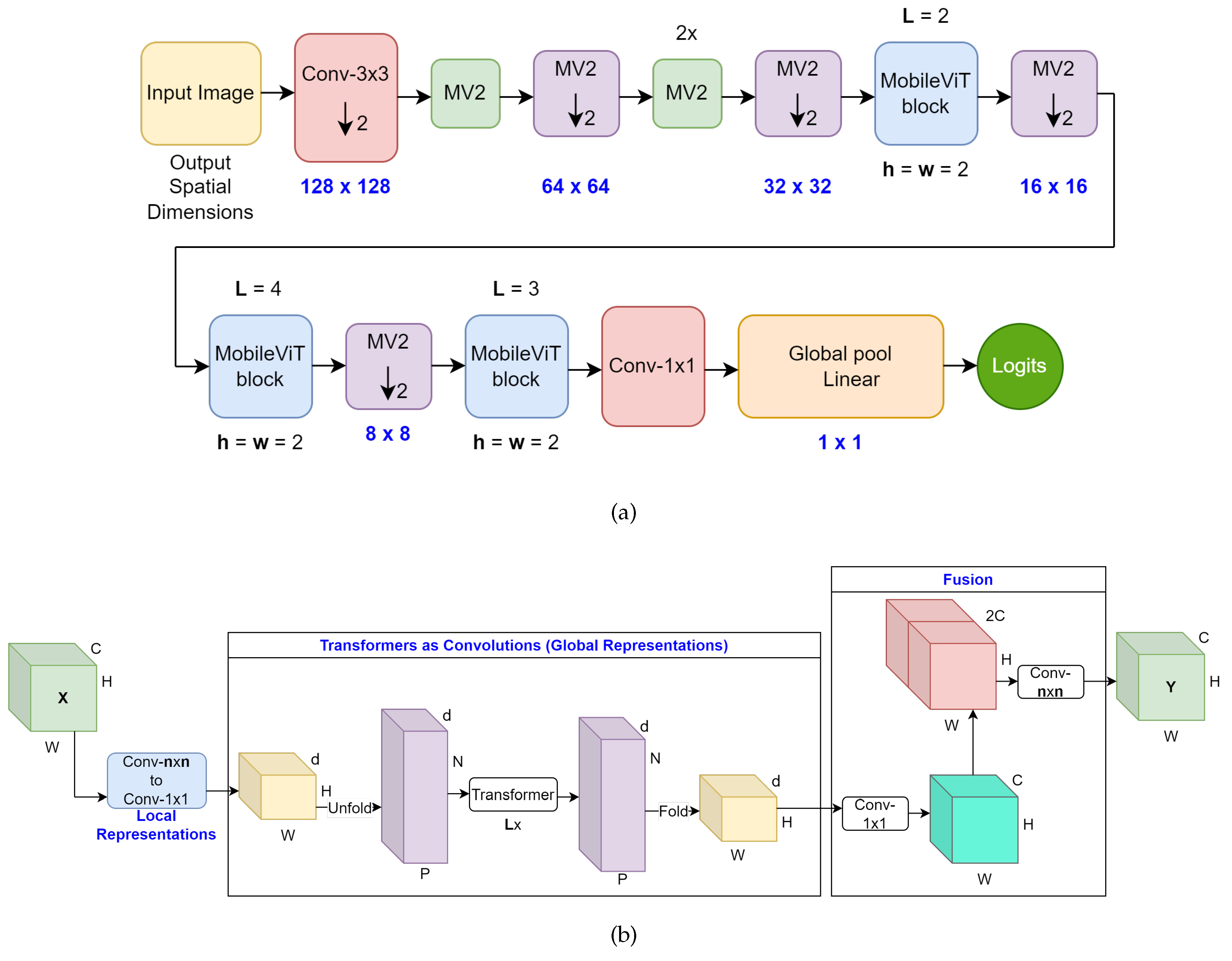
The overall architecture of the model is displayed in
Figure 2a. The architecture starts with a striped
convolutional layer. This layer is followed by four MobileNetv2 (MV2 blocks). The second and fourth blocks both use a stride of 2. These MV2 blocks are quite narrow and shallow which means they don’t significantly factor into the training parameter count. This is because their main responsibility is down-sampling. These blocks are followed by a MobileViT block which utilizes two transformer blocks that are represented by
. Also, the spatial dimensions of the feature maps are often multiples of 2. As a result, the height and width dimensions of the feature maps represented by
h and
w respectively are set to 2 at all spatial levels. Another MV2 block with stride of 2 is used before a MobileViT block with 4 transformer blocks. A dimension of 2 for the height and width spatial dimensions of the feature maps is applied. Then, a MV2 block with a stride of 2 is applied before the final MobileViT block with 3 transformer blocks and a dimension of 2 for the height and width spatial dimensions of the feature maps. Finally, a
convolutional layer and a global average pooling operation for spatial data are applied to produce the logits or the output of the last layer inside the model. Also, the output spatial dimensions of the model get smaller and smaller as the model gets closer to generating the logits. The output spatial dimensions used are
,
,
,
,
, and
.
The architecture of one MobileViT block is displayed in
Figure 2b. The MobileViT block receives an input tensor with the dimensions
C,
H, and
W which represent the channels, height, and width of the input tensor. Then, a
convolutional layer and a
convolutional layer are applied to the tensor in order to encode local spatial information and project the tensor to a high-dimensional space respectively. As a result, this produces a modified tensor with the dimensions
d,
H, and
W where
d is the size of the fixed dimensional space while the dimensions
H and
W represent the height and width of the input tensor. After this, the modified tensor is unfolded into non-overlapping flattened patches with the dimensions
d,
N, and
P which represent the size of the fixed dimensional space, the number of patches, and the product of the height and width of the pixels in the patches respectively. A stack of
L Transformer blocks where
L represents the number of transformer blocks is applied to the non-overlapping flattened patches to generate a new sequence of non-overlapping flattened patches with the same dimensions
d,
N, and
P. However, unlike ViT, MobileViT can remember the patch order and spatial order of pixels within each patch. The new sequence of flattened patches is then folded and projected to a high-dimensional space in order to make a tensor with dimensions
d,
H, and
W where
d represents the size of the fixed dimensional space. Then, a
convolutional layer is applied to the tensor to project it to a low-dimensional space with the dimensions
C,
H, and
W. After this, the newly formed tensor is concatenated with the input tensor to produce a new tensor with dimensions
,
H, and
W. Finally, an
convolutional layer is applied to fuse the concatenated features and generate the output tensor with dimensions
C,
H, and
W. MobileViT is a powerful model because it can achieve high performance with a reduced number of parameters relative to heavyweight ViTs and CNNs. It leverages the inherent advantages of both architectures.
While MobileVit can utilize both dependable aspects of CNN and Transformers, there are still potential improvements that can further optimize the MobileViT in order to boost its performance on geospatial datasets and reduce its training parameters. In this research, we explore these parameters in an incremental manner to further optimize this architecture by strategically replacing blocks that are used to extract higher order features.
3.2. Datasets
Models were trained on four Multi-Class Classification GIS datasets: AID [
26], EuroSAT [
27,
28], UC Merced [
29], and WHU-RS19 [
30,
31]. These datasets feature a diverse image sizes, spatial resolutions, image types, image formats, and labels. These statistics and data are displayed in
Table 1. The labels and their sequence numbers are provided in
Table 2. Due to the variety of datasets utilized for this project, we ensured that the better performance of our custom MobileViT variants was consistent across a wide range of labeled images.
The AID dataset is a large aerial image dataset that was formed by collecting images from Google Earth imagery. These Google Earth images are also post-processed with RGB renderings extracted from the original optical aerial images. The images of the AID dataset are labeled with 30 aerial scene class labels which is the most out of all the datasets. Also, there are 10,000 JPG images inside AID which have the size
, and an image resolution ranging from 0.5 m to 8 m.
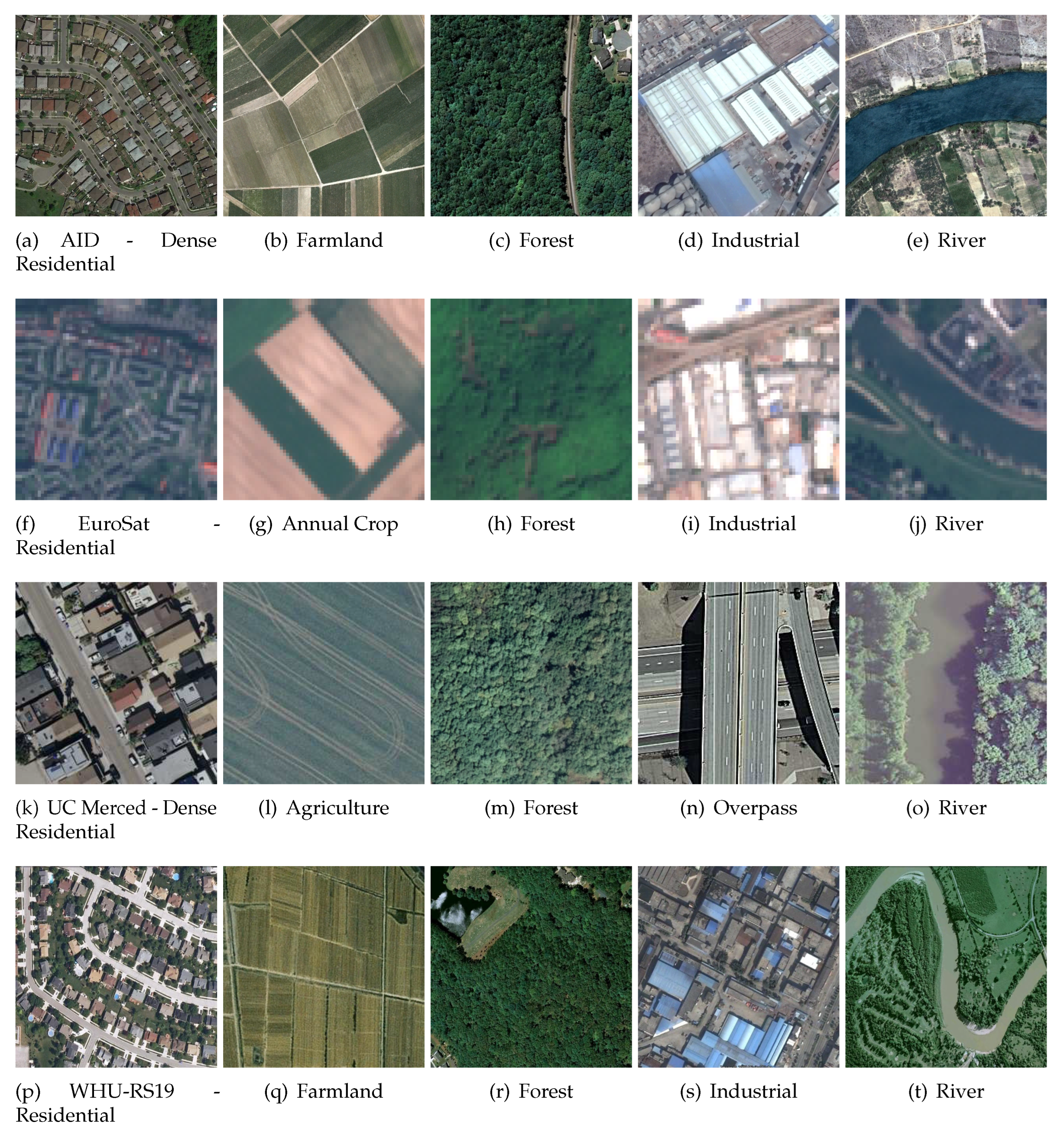
Figure 3a-
Figure 3e display five sample images from the AID dataset.
The EuroSAT dataset is a large-scale satellite multispectral image dataset that was collated by using Sentinel-2 satellite images that are accessible from the open-source Earth observation program Copernicus [
32]. Also, this dataset is unique because the images are multispectral and cover 13 spectral bands that are in the short infrared, near infrared, and visible parts of the spectrum. Our experiments used a smaller version of EuroSAT and the images of the dataset are labeled with nine class labels which is one less than the original and the least out of the four datasets. In addition, EuroSAT was the largest dataset as it contained 24,500 JPG images that have the size of 64 pixels by 64 pixels, and the image resolution 10 m.
Figure 3f-
Figure 3j display sample images from the EuroSAT datasets.
The UC Merced dataset [
29] is a large aerial image dataset that was formed by extracting a diverse range of smaller images from large images that were collated in the USGS National Map Urban Area Imagery Collection. The sizes of these smaller images are
, and the images come from different urban areas around the United States of America. The dataset’s images feature the smallest spatial resolution of the 4 datasets at 0.3 m, and they are the only dataset with TIF images. In addition, the dataset features images that belong to 21 classes, and there are 100 images per each image class which leads to a total of 2100 images in the dataset.
Figure 3k-
Figure 3o displays five sample images from the UC Merced dataset.
The WHU-RS19 dataset is a large-scale aerial image dataset that consists of satellite images that were collected from Google Earth. The dataset is similar to AID in that both datasets have the same image sizes (
), and they both originate from Google Earth imagery. In addition, WHU-RS19 is the smallest dataset out of the four datasets with 1005 JPG images. Also, the images in the dataset range have a spatial resolution of up to 0.5 m as well as a diverse range of orientations and illuminations. Also, the images of the dataset belong to 19 image classes.
Figure 3p-
Figure 3t displays sample images from the WHU-RS19 dataset.
3.3. Proposed lightweight transformer modifications
3.3.1. MobileVit-Avg
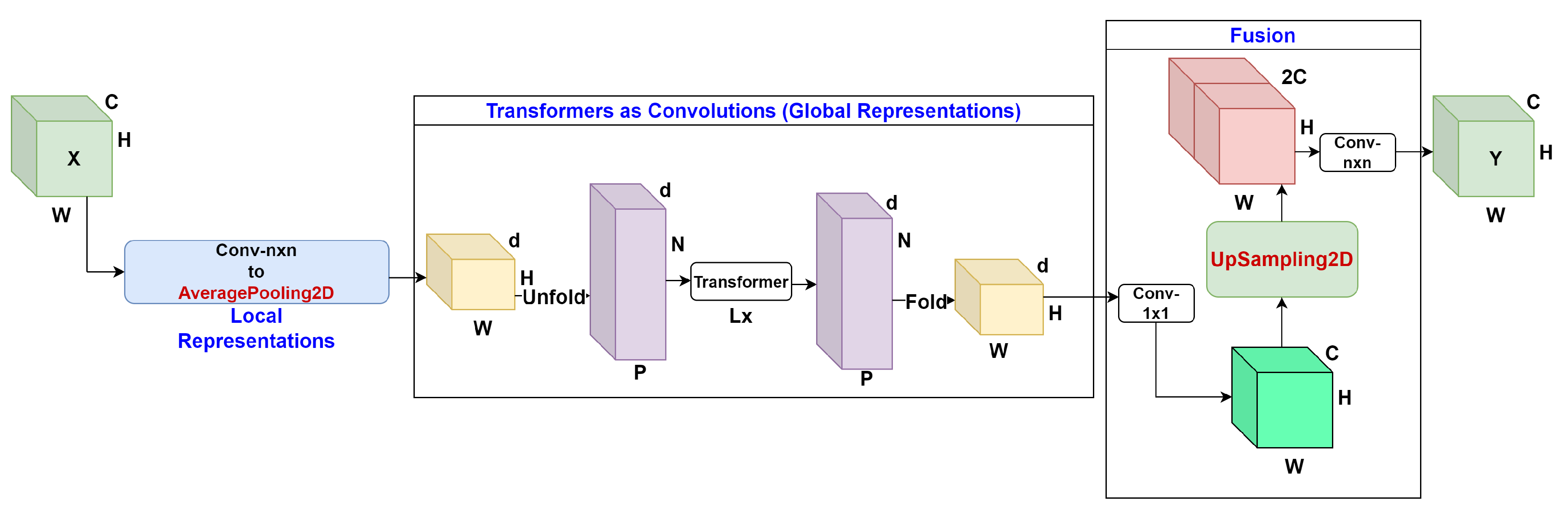
The first variant tested in our research is called MobileViT-Avg. To create this variant, a convolution layer in the Local Representations section of the MobileViT block was removed. An average pooling layer that features a pool_size of was added. A upsampling layer was introduced in between the folded global feature map that contains global features extracted by the Transformer block and the concatenate layer which combines the folded global feature map and the local features that were extracted using the convolution layer and average pooling layer. Following these changes, the number of training parameters was reduced significantly when compared to the benchmark ViT and MobileViT models. Across all 4 datasets, MobileViT-Avg had exactly 19,952 less parameters than MobileViT (1.52% decrease on average). In addition, MobileViT-Avg had 20,384,359 less parameters than ViT on average (94.04% decrease).
The architecture of MobileViT-Avg block is shown in
Figure 4. The MobileViT block receives an input tensor with the dimensions
C,
H, and
W which represent the channels, height, and width of the input tensor. Then, the model modifies the Local Representations section by using a
convolutional layer and an average pooling layer with a pool size of
that replaces the original
convolutional layer in order to encode local spatial information and project the tensor to a high-dimensional space respectively. This produces a modified tensor with the dimensions
d,
H, and
W where
d is the size of the fixed dimensional space. The modified tensor is unfolded into non-overlapping flattened patches with the dimensions
d,
N, and
P where
N and
P represents the number of patches, and the product of the height and width of the pixels in the patches respectively. A stack of
L number of Transformer blocks is applied to the non-overlapping flattened patches to generate a new sequence of non-overlapping flattened patches with the same dimensions
d,
N, and
P. This new sequence of flattened patches is folded and projected to a high-dimensional space in order to make a tensor with dimensions
d,
H, and
W. A
convolutional layer is applied to the tensor to project it to a low-dimensional space with the dimensions
C,
H, and
W. The tensor is then fed into an upsampling layer that helps balance the class labels followed by concatenation with the input tensor to produce a new tensor with dimensions
,
H, and
W. Finally, a
convolutional layer is applied to fuse the concatenated features and generate the output tensor with same dimensions
C,
H, and
W.
3.3.2. MobileViT-Depth
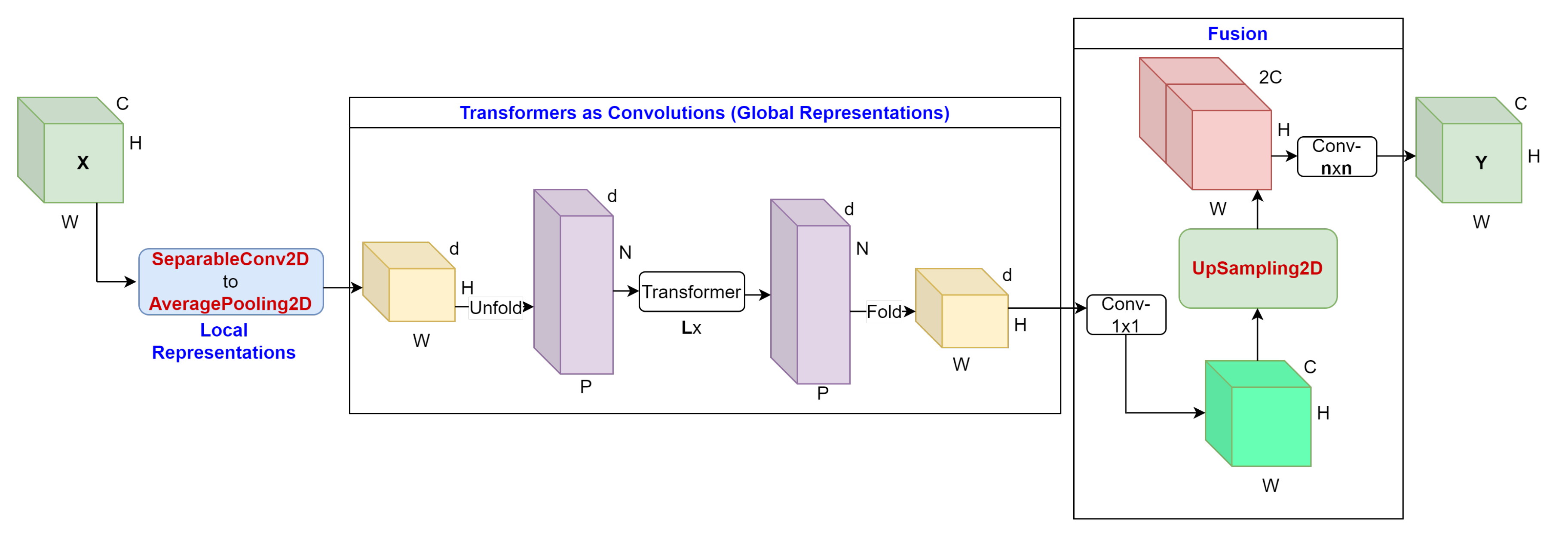
The second variant that was created is called MobileViT-Depth. To create this variant, we first started with the MobileViT-Avg architecture which contains the average pooling and upsampling layers as a base. Then, we further modified the MobileViT block inside the model by replacing the first convolution layer that takes in the input tensor in order to generate Local Representations with a depthwise separable convolution layer. After the changes were made, the reduction of training parameters for the MobileViT-Depth model was greater than the decrease achieved for the MobileViT-Avg model. When compared to the ViT model, MobileViT-Depth had 20,509,607 less parameters than ViT on average (94.62% decrease). When compared to the MobileViT model, MobileViT-Depth had exactly 145,200 less parameters than MobileViT across all 4 datasets (11.06% decrease).
The architecture of MobileViT-Depth block is shown in
Figure 5. This block receives an input tensor with the dimensions
C,
H, and
W. Then, the model modifies the Local Representations section by using a
separable convolutional layer instead of a regular convolutional layer as well as an average pooling layer with a pool size of
in order to encode local spatial information and project the tensor to a high-dimensional space respectively. This produces a modified tensor with the dimensions
d,
H, and
W which passes through the Transformer layers as explained in the previous MobileViT-Avg section. The new sequence of flattened patches is folded and projected to a high-dimensional space in order to make a tensor with dimensions
d,
H, and
W. Then, a
convolutional layer is applied to the tensor to project it to a low-dimensional space with the dimensions
C,
H, and
W. The tensor is then fed into an upsampling layer which was also added in the previous iteration of MobileVit-Avg that helps balance the class labels.
3.3.3. MobileVit-Shuffle
For the first two MobileViT variants, it’s important to note that we only modified the MobileViT block architecture and left the overall architecture intact. However, for our last variant, we modified the MobileViT block architecture and the overall MobileViT architecture by inserting a custom block into the overall architecture. The third variant that we generated is called MobileViT-Shuffle. The custom ShuffleNet block replaces the final MobileViT block as shown in
Figure 2a. This ShuffleNet block sets the default kernel size of its layers to be
, and it sets the default number of filters to be 320.
The custom ShuffleNet block mentioned in the previous paragraph can be seen in
Figure 6. This block consists of two pathways of layers that are fused together in order to generate the output tensor. Both pathways receive an input tensor with the dimensions
C,
H, and
W. The first pathway of layers is called
A, and it starts with feeding the input tensor into a
depthwise convolution layer. Then, the output from that initial layer is processed by a batch normalization layer as well as a
convolution layer. Finally, the pathway ends with the output being processed by another batch normalization and a ReLU layer. The second pathway of layers is labeled with
B, and it starts with feeding the input tensor into a
convolution layer. The output from the initial layer is processed by a batch normalization layer and a ReLU Layer. Then, the new output is processed by a
depthwise convolution layer as well as another
convolution layer. The activation map is then processed by another batch normalization layer and another ReLU layer. To fuse the two pathways, a concatenate layer is utilized. The fusion results in an output tensor with dimensions
C,
H, and
W. After these changes were made, the reduction in training parameters for the MobileViT-Shuffle variant was greater than the training parameter decrease for the other two variants. Across the 4 datasets, MobileViT-Shuffle had 20,598,679 less parameters than ViT on average (95.03% decrease). Also, MobileViT-Shuffle had exactly 234,272 less parameters than MobileViT across all 4 datasets (17.85% decrease).
The total number of training parameters for each model architecture trained across the 4 GIS datasets AID, EuroSAT, UC Merced, and WHU-RS19 is summarized in the
Table 3. All of the hyperparameters except number of classes and train-test splits used by the model don’t influence the number of training parameters, so there are only 4 entries for each model. An observable trend in the table is that the training model parameters for each architecture increases on datasets that have a larger number of image labels. This shows that each model’s output layer which maps to a differing number of image classes for each dataset slightly influences the training parameters inside each model.
4. Results
For the training and evaluation stage of the completed model architectures, a group of four experiments were devised where each experiment corresponded to one of the four datasets that we were going to train and evaluate the models on. This was followed by application of each representative architecture which includes the two benchmarks ViT and MobileViT along with the three MobileViT variants to all of the datasets. Multiple train-test splits for each model architecture was also introduced to ascertain if the models could achieve a high level of performance with lesser amounts of training data. The train-test splits used were 20%-80%, 40%-60%, 50%-50%, and 60%-40% respectively. Hence, each experimental group corresponding to one of the four datasets had 20 models were used for training which can be calculated by multiplying the number of model architectures (5) and the number of train-test splits (4). In summary, a total of 80 models which can be calculated by multiplying the number of model architectures (five), the number of train-test splits (four), and the number of datasets (four). All experiments were conducted on Blugold Center for High Performance Computing using NVIDIA Tesla V100 GPU with 32GB memory and AMD EPYC CPU at 2.35 GHz.
Data augmentation for the training images started with resizing all of the images to
followed by randomly flipping those images along a horizontal axis. The images were randomly rotated before being randomly zoomed into during the training process. Hyperparameters were configured in order to control the training process. The number of epochs was kept constant at 500, and the batch size was kept constant at 64. Also, all of the models used an Adam optimizer to help change the weights and loss rates. For this optimizer, the learning rate was set to 0.001 which allowed for slow and precise learning. The weight decay was set to 0.0001 in order to regularize the neural network by adding a penalty to the loss function. The only hyperparameter that we varied across the models was the number of classes or labels because each dataset has a different number of image classes. This hyperparameter played a role in influencing the total number of training parameters because it modified the size of the output Dense layer in the ViT models. The training and validation accuracy for all model variants are shown in
Table 4.
For the AID experiment group the MobileViT variants Avg, Depth, and Shuffle outperformed the ViT model across all of the splits. We noted a consistent trend among all the architectures where the
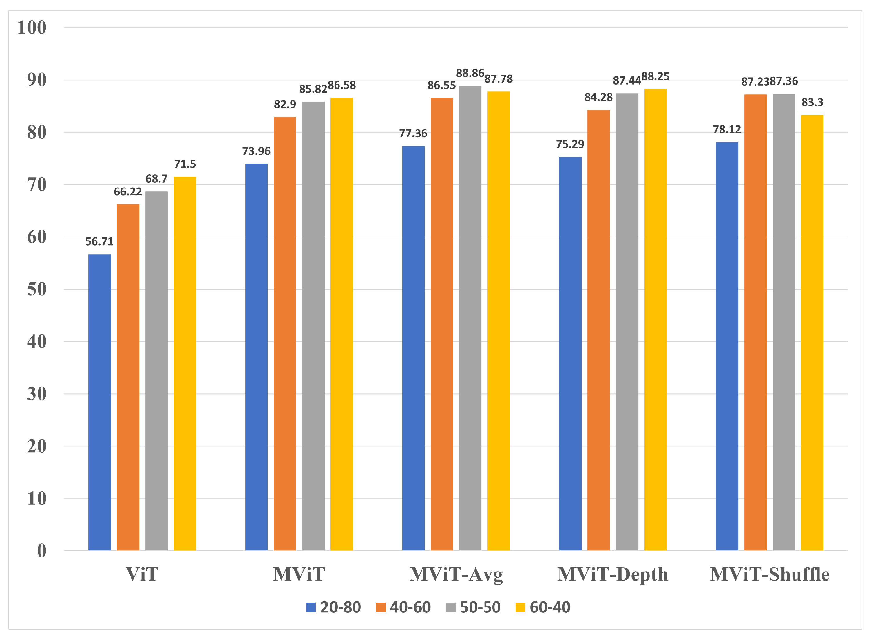
split was usually the highest performing model when compared to the other splits of the same architecture with validation accuracy of 88.86% that outperformed ViT’s best validation accuracy by 17.36% and the benchmark MobileViT’s validation accuracy by 2.28%. The class-based performance for 50-50 AID testing dataset is shown in
Table 5. In addition, the variants were able to achieve this result despite having 94.03%, 94.60%, and 95.01% less parameters respectively. Also, each MobileViT variant’s best split outperformed the original MobileViT’s best split. Moreover, this outcome was achieved despite the Avg, Depth, and Shuffle variants having 1.52%, 11.04%, and 17.81% less parameters respectively.
Figure 7 further shows a comparison of the validation accuracy for the AID dataset used in this study.
Table 5 displays the per-class validation accuracy of the 50-50 split using AID. We notice that several classes that performed poorly using ViT show significant improvements when MobileViT variants are used. For example, the accuracy of Airports (class 0) jumped from 40% to 91.11% for MobileViT-Shuffle. Similar trends were observed for Farmlands (class 10), Mountains (class 15), Parks (class 16), Storage Tanks (class 28) and Viaduct (class 29). All models found it challenging to classify a Square (class 26). This could be because square was a shape containing several sub-classes like buildings and airports making it challenging to group them into a separate class.
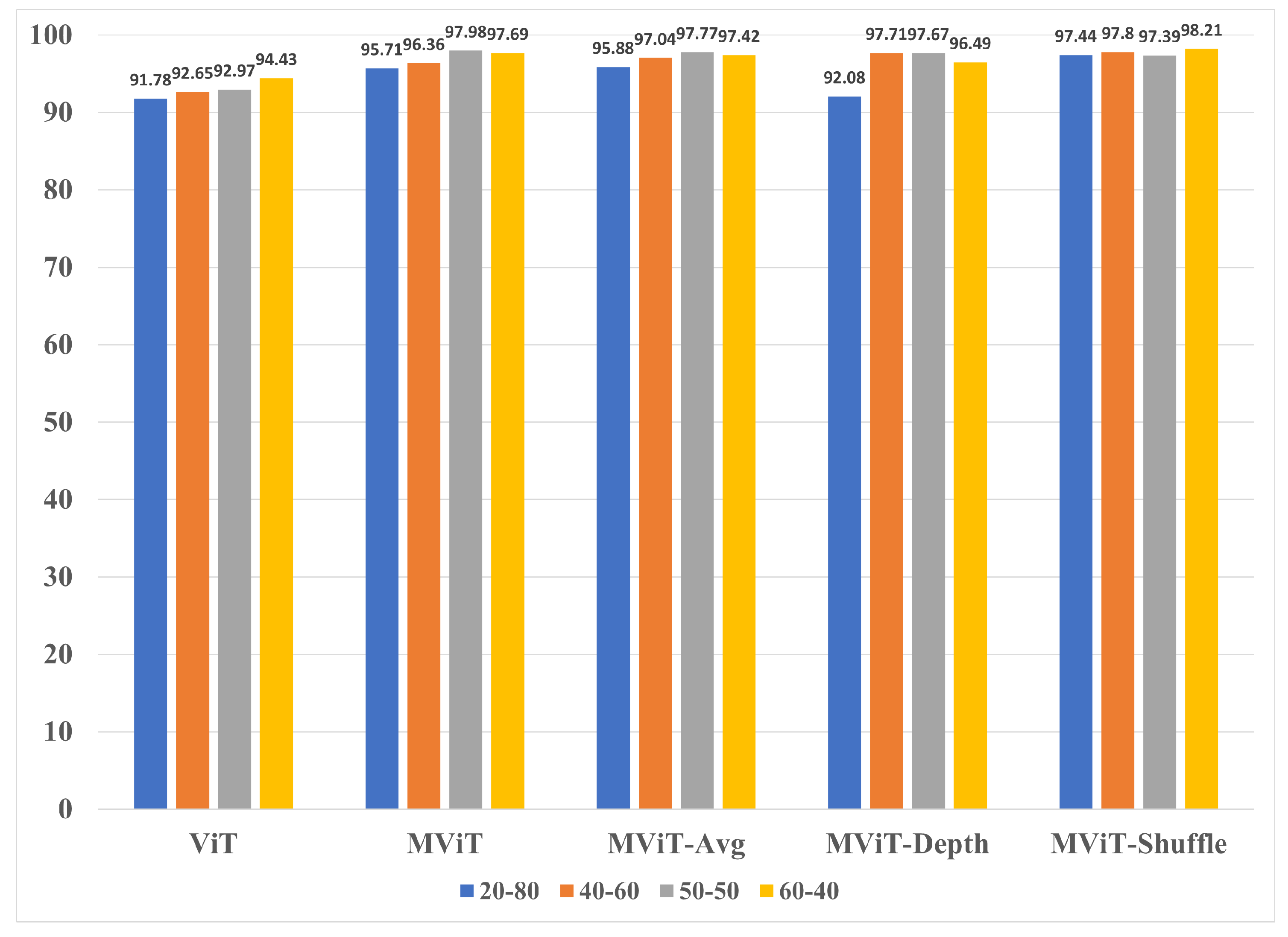
The results for the EuroSAT experiment group established the
split was usually the highest performing model although the 50-50 split was not far behind as shown in
Table 4. The MobileViT variants Avg, Depth, and Shuffle also outperformed the ViT model across all of the splits. The MobileViT variant Shuffle was the best performing model with an accuracy of 98.21% that outperformed ViT’s best split by 3.78% and the benchmark MobileViT’s best split by 0.23%. Moreover, Shuffle was able to outperform the benchmark MobileViT model despite being the most lightweight variant that has 17.90% less parameters than the MobileViT model. The class-based performance for 60-40 EuroSAT testing dataset is shown in
Table 6 along with the validation accuracy graphs in
Figure 8. Unlike the AID dataset where we observed noticeable improvements when shifting from ViT to MobileViT variants, the accuracy for EuroSAT was mostly consistent with minor increase in accuracy. For example, the largest jump in accuracy was for Highways (class 3) where ViTs achieved 70% compared to MobileViT-Shuffle which reached 82.5%. Other than that, the accuracy was mostly consistent with the highest positive change being 5.25% for River (class 7). A contributing factor to this trend may have to do with EuroSAT’s data resolution being significantly lower than the remaining datasets however further investigation is needed to confirm this trend.
The results for the UC-Merced experiment group show that the
split model was usually the highest performing model, however following a similar pattern, the
split performed well too. In fact, the best performing model was in the
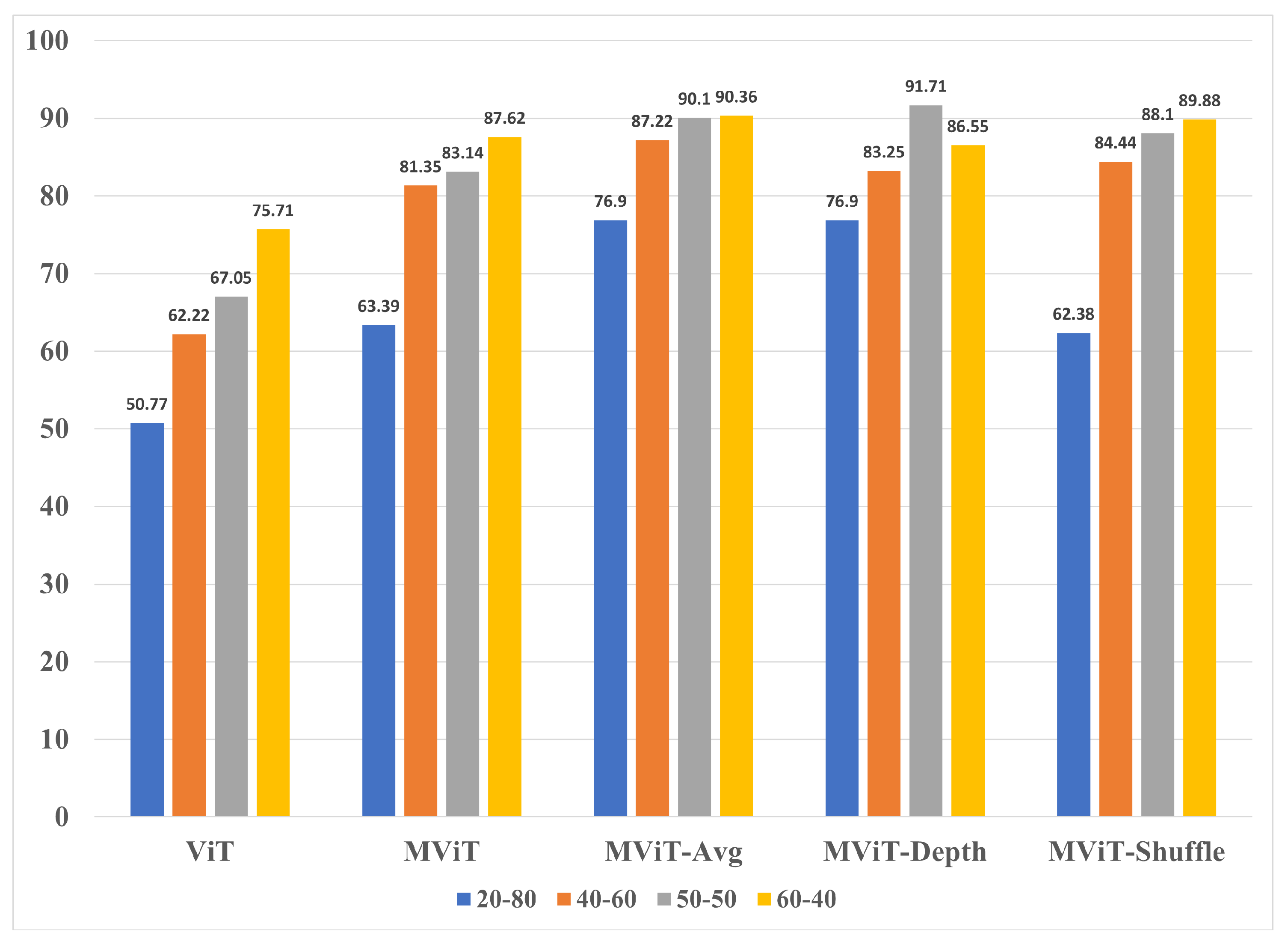
split. This was MobileViT-Depth with an accuracy of 91.71% that outperformed ViT’s best split by 16% and the benchmark MobileViT’s best split by 4.09% when compared to the other splits of the same architecture. Following previous trends we also observed that the MobileViT variants Avg, Depth, and Shuffle outperformed the ViT model across all of the splits. Also, we found that the best splits for the Avg, Depth, and Shuffle variants outperformed the best split of the MobileViT benchmark model. The graph showing validation accuracies of UC-Merced can be seen in
Figure 9. The class-based validation performance for
UC-Merced housing the best performing model is shown in
Table 7. Unlike the AID dataset we noticed substantial improvements with the MobileViT-derived architecture across multiple classes. For example, a comparison between ViT and MobileViT-Shuffle revealed a 46% increase for Dense Residential (class 6), 42% increase for Golf course (class 9), 46% increase for Overpass (class 14), 66% increase for Sparse Residential (class 18), 44% increase for Storage Tanks (class 19) and a 42% increase for Tennis Course (class 20). In fact the highest increase in accuracy was observed in residential classes showing that the Mobile-Vit architectures are capable to accurately differentiate between different types of housing structures.
The results for the WHU-RS19 experiment group are shown reveal that the
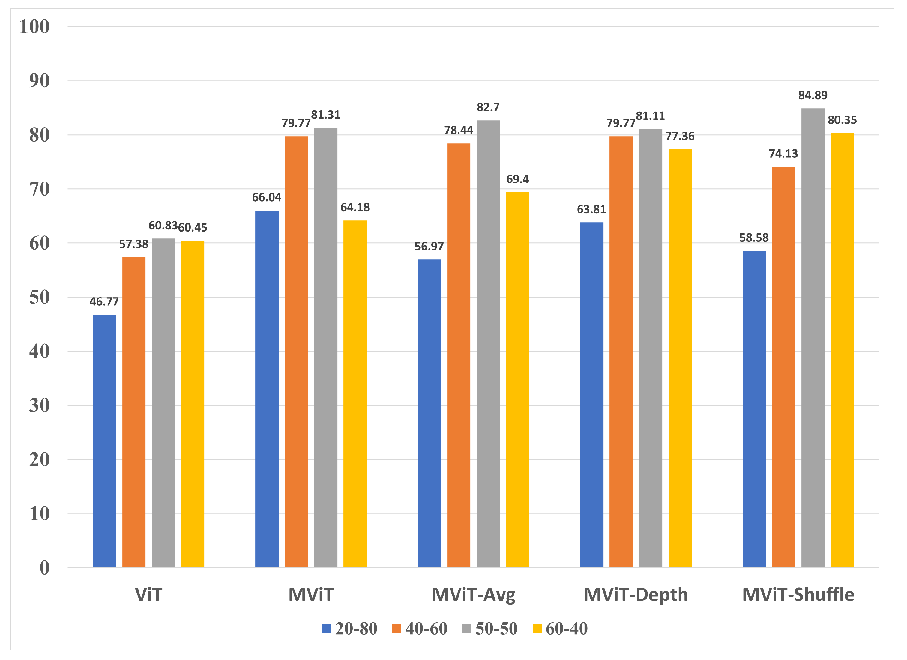
split was the highest performing model when compared to the other splits of the same architecture. In a similar trend, the MobileViT variants Avg, Depth, and Shuffle outperformed the ViT model across all of the splits. MobileViT-Shuffle was the highest performing model with an accuracy of 84.89% that outperformed ViT’s best split by 24.44% and MobileViT’s best split by 3.58%. Moreover, Shuffle achieved this result despite being the most lightweight architecture in terms of number of trainable parameters out of all of the five representative model architectures. The class-based performance for
WHU-RS19 dataset is shown in
Table 8 along with the validation accuracy graphs in
Figure 10.We also note that like AID, and UC-Merced, using the MobileNet variants resulted in significant accuracy increase for several classes. To summarize,
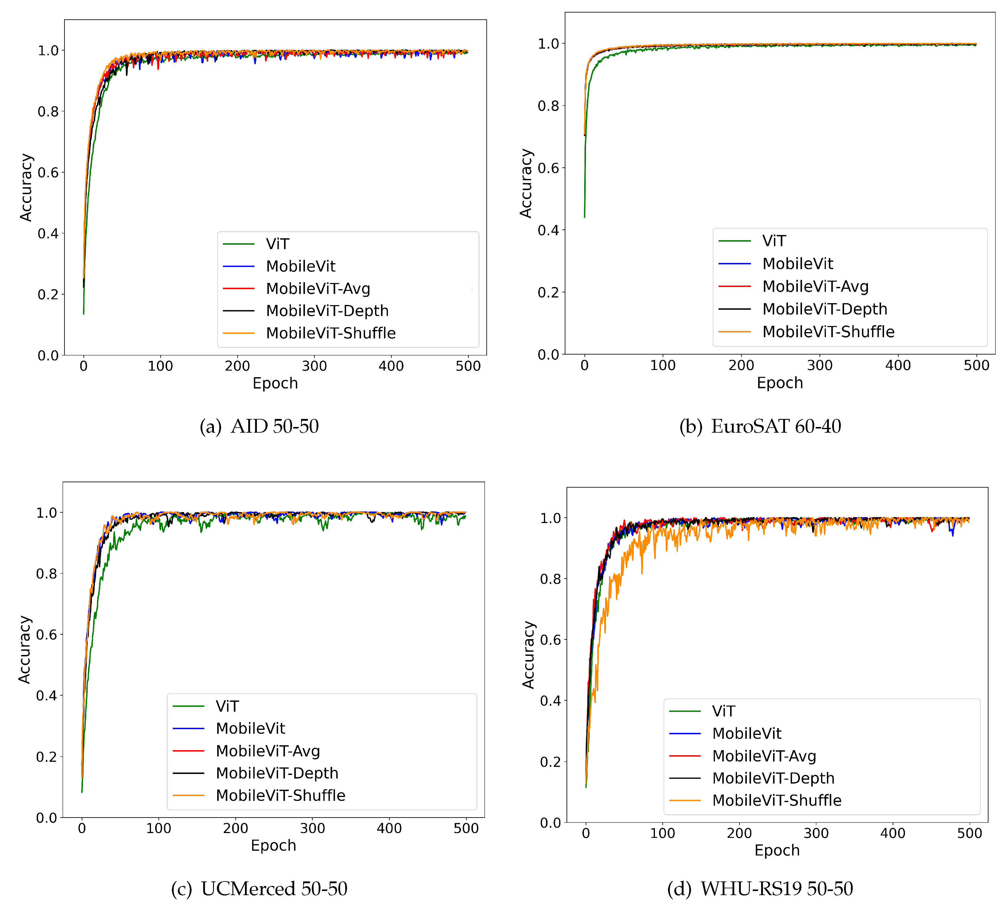
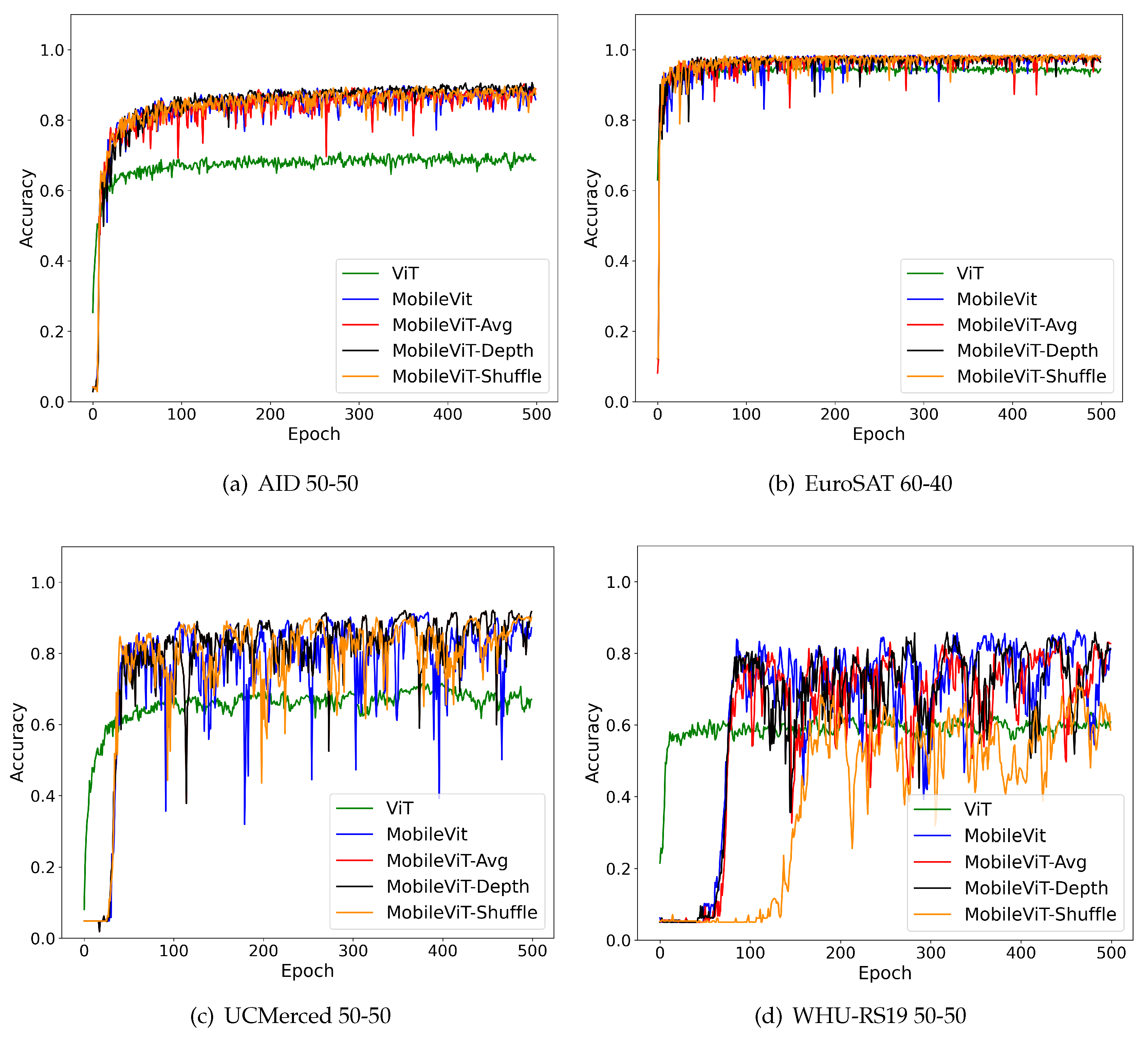
Figure 11 and
Figure 12 shows the training and validation accuracy scores for the best split across all four datasets. While training accuracy in most cases remained consistently high, we noticed significant variation in the validation accuracy mostly in UC-Merced and WHU-RS19 datasets. However, the models were able to converge to an acceptable value at the end of 500 epochs.
5. Discussion
Our experiments revealed that a confluence of modern transformer architecture with lightweight CNN frameworks have the potential to yield superior outcomes. As a result, it opens up a vast array of possibilities where deep learning can be made optimized based and generalized across multiple domains. It is worth noting that along with the successful three variants we also explored other modifications in CNN architectures which did not have a similar outcome. In this section we will list those variants that were unable to boost or preserve accuracy.
Five of the unsuccessful MobileViT variants involved removing entire MobileViT blocks from the overall architecture of the benchmark model in an attempt to lower training parameters. All of these variants had their respective architectures configured on the UC-Merced dataset and a train-test split. One of these variants had a modified structure that removed the first MobileViT block from the overall MobileViT architecture. The removal resulted in the variant having 1,112,725 trainable parameters which meant the number of training parameters was reduced by 15.24% relative to the benchmark MobileViT architecture. However, this variant could not maintain the benchmark’s performance as it achieved an accuracy of 78.00% which was 9.14% lower than the 87.14% accuracy achieved by MobileViT. In addition, we created another variant that removed the last MobileViT from the overall MobileViT architecture. The removal resulted in the variant having 687,605 training parameters which meant the number of training parameters was reduced by 47.62% relative to the benchmark. Unfortunately, the variant failed to achieve the benchmark’s accuracy as it attained the testing accuracy of 83.24% which was 3.90% lower than the benchmark’s accuracy.
The other two out of the five variants which removed entire blocks from the overall architecture of the benchmark model focused on eliminating some of the inverted residual blocks. One of these variants had a modified architecture that removed the first inverted residual MV2 block from the overall benchmark architecture. This removal resulted in the variant having 1,309,501 training parameters which meant the number of training parameters was reduced by 0.25%. However, the variant could not achieve the benchmark’s performance as it attained an accuracy of 84.19% which was 2.95% lower than the benchmark’s accuracy. In addition, we also created another variant which removed the second inverted residual MV2 block from the overall benchmark architecture. This elimination resulted in the variant having 1,309,501 training parameters which meant the number of training parameters was reduced by 0.25%. Unfortunately, the variant also could not achieve the benchmark’s accuracy as it attained an accuracy of 84.19% which was 2.95% lower than the benchmark’s performance on the same dataset and train-test split.
Our final failed variant featured changes that were similar to the more fine-tuned and subtle manipulations made on the benchmark MobileViT model to generate the three successful variants. This variant was also configured on the UC-Merced dataset and a train-test split before being compared to the original MobileViT benchmark configured on the same dataset and train-test split. It had a modified structure that replaced the last convolutional layer in the MobileViT block’s Fusion section with a Depthwise Separable Convolution layer. In addition, this variant also had the changes from the MobileViT-Avg variant which include the average pooling layer that replaced the second convolutional layer in the MobileViT block’s local representations section as well as an added UpSampling layer in the MobileViT block’s Fusion section. This replacement resulted in the variant having 1,042,309 training parameters which meant the number of training parameters was reduced by 20.60%. However, the variant could not attain the benchmark’s accuracy as it attained an accuracy of 77.81% which was 9.33% lower than the benchmark’s performance.
6. Conclusions
This work presented three new variants of the benchmark MobileViT model called MobileViT-Avg, MobleViT-Depth, and MobileViT-Shuffle as well as their training and evaluation results on 4 GIS datasets namely AID, EuroSAT, UC-Merced, and WHU-RS19. The results show that the three variants outperform the benchmark MobileViT and ViT architectures despite having a significantly smaller footprint. As a result, we can reason that our methods retained the benefits of CNNs and Transformers while replacing some of the expensive deep learning computational layers by boosting accuracy and reducing the training parameters. However, as highlighted in the discussions, these changes should not use the effectiveness of diverse activation maps. This would then have an adverse effect on the model’s performance. Future work would explore further modifications mostly to optimize the Transformer layers. The model performance will also be integrated with ImageNet dataset to explore possibilities of transfer learning. Finally an endeavor to create usable GIS deep learning transformer based models will be developed for the community by attempting to train and evaluate these models on a merged dataset composed of images from the AID, EuroSAT, UC-Merced, and WHU-RS19 datasets to ensure the continuity and validity of our results.
Funding
This article was funded by National Science Foundation Research Experience of Undergraduates (REU) grant OAC-2150191. The computational resources of the study were provided by the Blugold Center for High-Performance Computing under NSF grant CNS-1920220.
Data Availability Statement
Conflicts of Interest
The authors declare no conflict of interest.
Abbreviations
The following abbreviations are used in this manuscript:
| CNN |
Convolutional Neural Networks |
| ViT |
Vision Transformer |
Appendix A
Appendix A.1
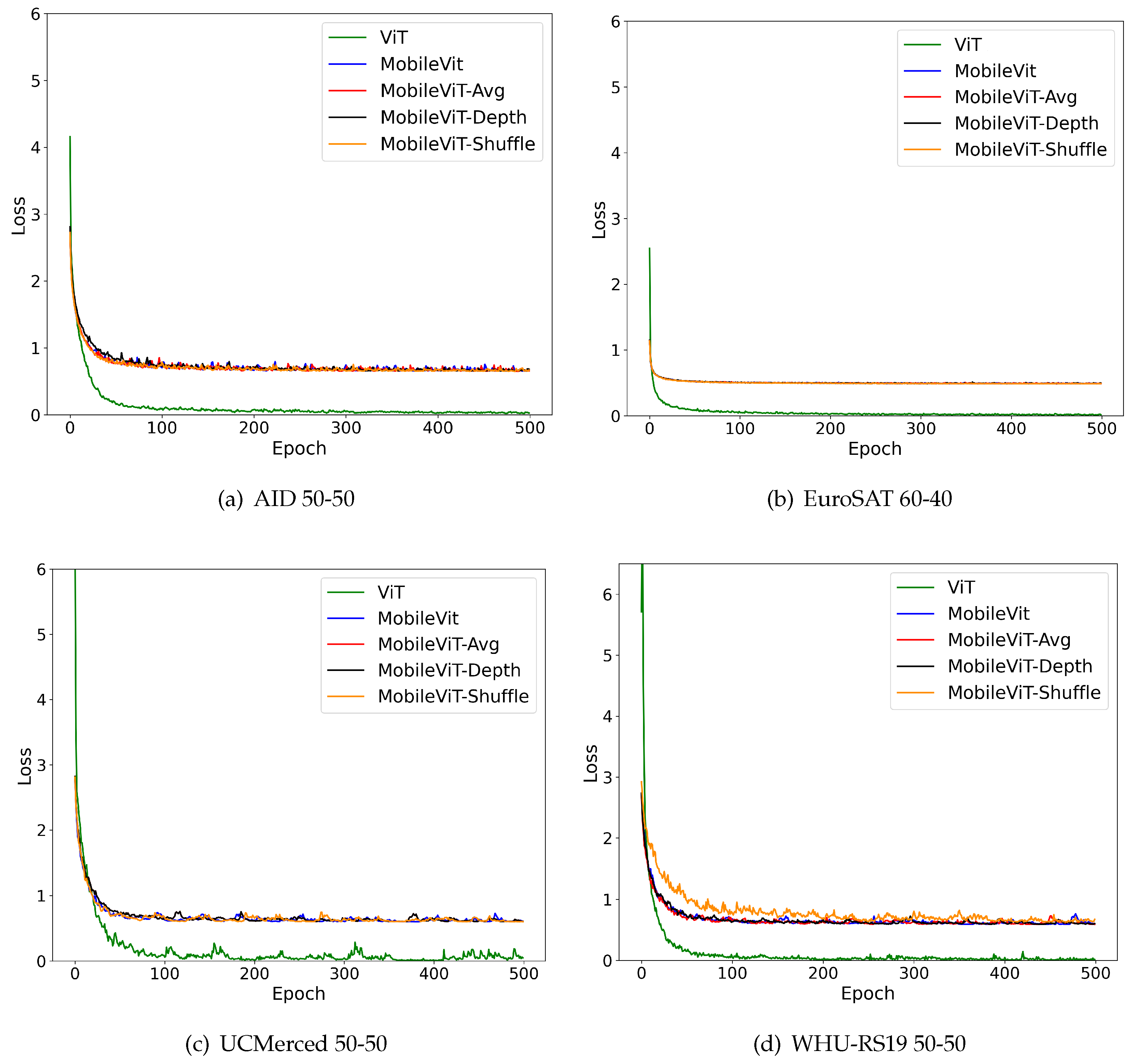
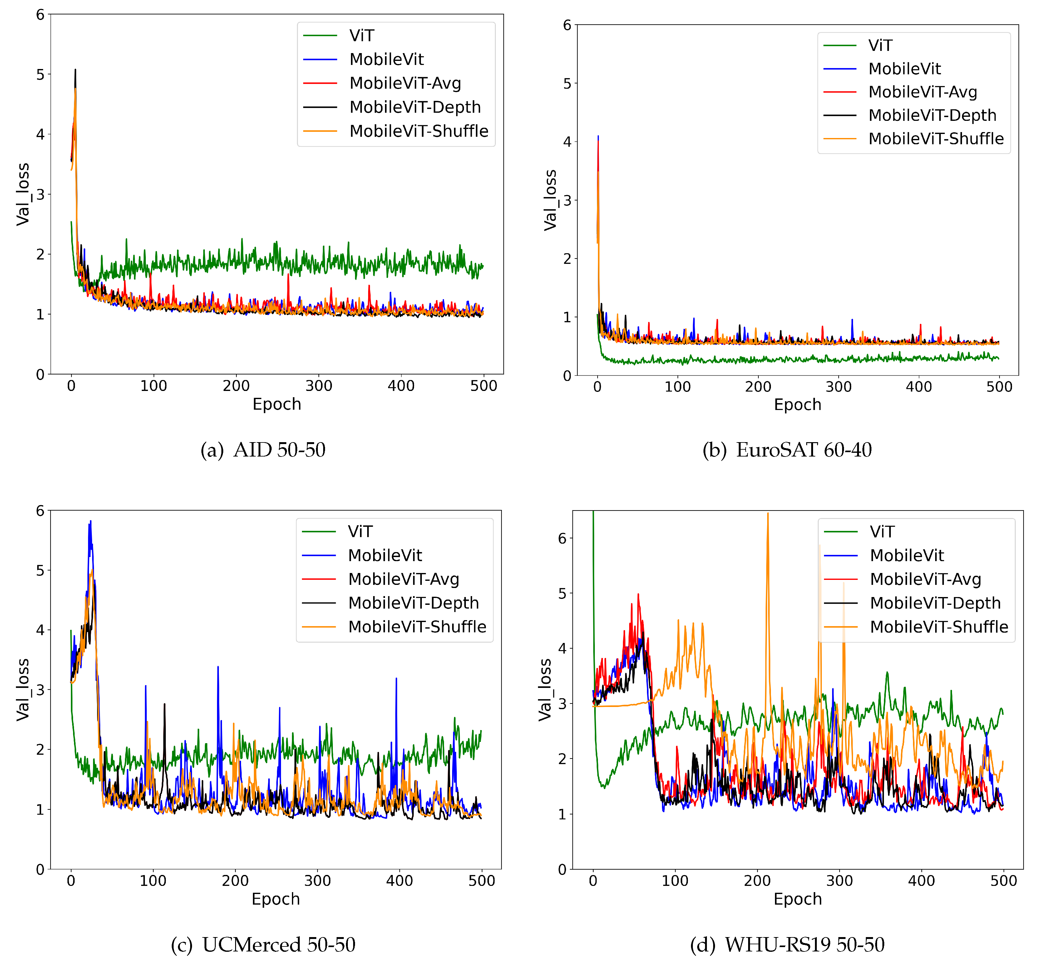
Here are the loss graphs of the models found using the best splits.
Figure A1.
Training loss graphs of best models evaluated in this study.
Figure A1.
Training loss graphs of best models evaluated in this study.
Figure A2.
Validation loss graphs of best models evaluated in this study.
Figure A2.
Validation loss graphs of best models evaluated in this study.
References
- Chowdhary, K.; Chowdhary, K. Natural language processing. Fundamentals of artificial intelligence 2020, pp. 603–649.
- Krizhevsky, A.; Sutskever, I.; Hinton, G.E. Imagenet classification with deep convolutional neural networks. Advances in neural information processing systems 2012, 25.
- Madurapperuma, B.; Rozario, P.; Oduor, P.; Kotchman, L. Land-use and land-cover change detection in Pipestem Creek watershed, North Dakota. International Journal of GEOMATICS and GEOSCIENCES 2015, 5, 416–426.
- Haffner, M.; DeWitte, M.; Rozario, P.F.; Ovando-Montejo, G.A. A Neural-Network-Based Landscape Search Engine: LSE Wisconsin. Applied Sciences 2023, 13, 9264. [CrossRef]
- Rozario, P.F.; Oduor, P.; Kotchman, L.; Kangas, M.; others. Quantifying spatiotemporal change in landuse and land cover and accessing water quality: A case study of Missouri watershed james sub-region, north Dakota. Journal of Geographic Information System 2016, 8, 663. [CrossRef]
- Kussul, N.; Lavreniuk, M.; Skakun, S.; Shelestov, A. Deep learning classification of land cover and crop types using remote sensing data. IEEE Geoscience and Remote Sensing Letters 2017, 14, 778–782. [CrossRef]
- Ma, L.; Liu, Y.; Zhang, X.; Ye, Y.; Yin, G.; Johnson, B.A. Deep learning in remote sensing applications: A meta-analysis and review. ISPRS journal of photogrammetry and remote sensing 2019, 152, 166–177. [CrossRef]
- Hong, D.; Gao, L.; Yokoya, N.; Yao, J.; Chanussot, J.; Du, Q.; Zhang, B. More diverse means better: Multimodal deep learning meets remote-sensing imagery classification. IEEE Transactions on Geoscience and Remote Sensing 2020, 59, 4340–4354. [CrossRef]
- Lin, T.; Wang, Y.; Liu, X.; Qiu, X. A survey of transformers. AI Open 2022. [CrossRef]
- Carion, N.; Massa, F.; Synnaeve, G.; Usunier, N.; Kirillov, A.; Zagoruyko, S. End-to-end object detection with transformers. European conference on computer vision. Springer, 2020, pp. 213–229. [CrossRef]
- Mehta, S.; Rastegari, M. Mobilevit: light-weight, general-purpose, and mobile-friendly vision transformer. arXiv preprint 2021. arXiv:2110.02178.
- Gomes, R.; Rozario, P.; Adhikari, N. Deep learning optimization in remote sensing image segmentation using dilated convolutions and ShuffleNet. 2021 IEEE International Conference on Electro Information Technology (EIT). IEEE, 2021, pp. 244–249. [CrossRef]
- Dimitrovski, I.; Kitanovski, I.; Kocev, D.; Simidjievski, N. Current trends in deep learning for Earth Observation: An open-source benchmark arena for image classification. ISPRS Journal of Photogrammetry and Remote Sensing 2023, 197, 18–35. [CrossRef]
- Reedha, R.; Dericquebourg, E.; Canals, R.; Hafiane, A. Transformer neural network for weed and crop classification of high resolution UAV images. Remote Sensing 2022, 14, 592. [CrossRef]
- Bazi, Y.; Bashmal, L.; Rahhal, M.M.A.; Dayil, R.A.; Ajlan, N.A. Vision transformers for remote sensing image classification. Remote Sensing 2021, 13, 516. [CrossRef]
- Guo, J.; Jia, N.; Bai, J. Transformer based on channel-spatial attention for accurate classification of scenes in remote sensing image. Scientific Reports 2022, 12, 15473. [CrossRef]
- Cheng, Q.; Li, X.; Zhu, B.; Shi, Y.; Xie, B. Drone detection method based on MobileViT and CA-PANet. Electronics 2023, 12, 223. [CrossRef]
- Wan, Z.; Wan, J.; Cheng, W.; Yu, J.; Yan, Y.; Tan, H.; Wu, J. A Wireless Sensor System for Diabetic Retinopathy Grading Using MobileViT-Plus and ResNet-Based Hybrid Deep Learning Framework. Applied Sciences 2023, 13, 6569. [CrossRef]
- Xie, S.; Girshick, R.; Dollár, P.; Tu, Z.; He, K. Aggregated residual transformations for deep neural networks. Proceedings of the IEEE conference on computer vision and pattern recognition, 2017, pp. 1492–1500.
- Hu, J.; Shen, L.; Sun, G. Squeeze-and-excitation networks. Proceedings of the IEEE conference on computer vision and pattern recognition, 2018, pp. 7132–7141.
- Howard, A.G.; Zhu, M.; Chen, B.; Kalenichenko, D.; Wang, W.; Weyand, T.; Andreetto, M.; Adam, H. Mobilenets: Efficient convolutional neural networks for mobile vision applications. arXiv preprint : 2017. arXiv:1704.04861.
- Zhang, X.; Zhou, X.; Lin, M.; Sun, J. Shufflenet: An extremely efficient convolutional neural network for mobile devices. Proceedings of the IEEE conference on computer vision and pattern recognition, 2018, pp. 6848–6856.
- Wadekar, S.N.; Chaurasia, A. Mobilevitv3: Mobile-friendly vision transformer with simple and effective fusion of local, global and input features. arXiv preprint 2022. arXiv:2209.15159.
- Mehta, S.; Rastegari, M. Separable self-attention for mobile vision transformers. arXiv preprint 2022. arXiv:2206.02680.
- Dosovitskiy, A.; Beyer, L.; Kolesnikov, A.; Weissenborn, D.; Zhai, X.; Unterthiner, T.; Dehghani, M.; Minderer, M.; Heigold, G.; Gelly, S.; others. An image is worth 16x16 words: Transformers for image recognition at scale. arXiv preprint 2020. arXiv:2010.11929.
- Xia, G.S.; Hu, J.; Hu, F.; Shi, B.; Bai, X.; Zhong, Y.; Zhang, L.; Lu, X. AID: A benchmark data set for performance evaluation of aerial scene classification. IEEE Transactions on Geoscience and Remote Sensing 2017, 55, 3965–3981. [CrossRef]
- Helber, P.; Bischke, B.; Dengel, A.; Borth, D. Introducing EuroSAT: A Novel Dataset and Deep Learning Benchmark for Land Use and Land Cover Classification. IGARSS 2018-2018 IEEE International Geoscience and Remote Sensing Symposium. IEEE, 2018, pp. 204–207.
- Helber, P.; Bischke, B.; Dengel, A.; Borth, D. Eurosat: A novel dataset and deep learning benchmark for land use and land cover classification. IEEE Journal of Selected Topics in Applied Earth Observations and Remote Sensing 2019.
- Yang, Y.; Newsam, S. Bag-of-visual-words and spatial extensions for land-use classification. Proceedings of the 18th SIGSPATIAL international conference on advances in geographic information systems, 2010, pp. 270–279. [CrossRef]
- Xia, G.S.; Yang, W.; Delon, J.; Gousseau, Y.; Sun, H.; MaÎtre, H. Structural high-resolution satellite image indexing; , 2010.
- Dai, D.; Yang, W. Satellite Image Classification via Two-Layer Sparse Coding With Biased Image Representation. IEEE Transactions on Geoscience and Remote Sensing 2011, 8, 173–176. [CrossRef]
- Gascon, F.; Cadau, E.; Colin, O.; Hoersch, B.; Isola, C.; Fernández, B.L.; Martimort, P. Copernicus Sentinel-2 mission: products, algorithms and Cal/Val. Earth observing systems XIX. SPIE, 2014, Vol. 9218, pp. 455–463. [CrossRef]
Figure 1.
Architecture of the Vision Transformer model
Figure 1.
Architecture of the Vision Transformer model
Figure 2.
(a) Overall architecture of Mobile-Friendly Vision Transformer (Mobile-ViT) and (b) shows the architecture of one MobileVit block in (a)
Figure 2.
(a) Overall architecture of Mobile-Friendly Vision Transformer (Mobile-ViT) and (b) shows the architecture of one MobileVit block in (a)
Figure 3.
Sample images from the four datasets used in this study.
Figure 3.
Sample images from the four datasets used in this study.
Figure 4.
Architecture of the proposed MobileVit-Avg Transformer block with changes in red.
Figure 4.
Architecture of the proposed MobileVit-Avg Transformer block with changes in red.
Figure 5.
Architecture of the proposed MobileVit-Depth Transformer block with changes in red.
Figure 5.
Architecture of the proposed MobileVit-Depth Transformer block with changes in red.
Figure 6.
Architecture of the ShuffleNet block that replaces the final MobileVit block to create final the MobileVit-Shuffle transformer variant
Figure 6.
Architecture of the ShuffleNet block that replaces the final MobileVit block to create final the MobileVit-Shuffle transformer variant
Figure 7.
Validation accuracy comparison of AID dataset.
Figure 7.
Validation accuracy comparison of AID dataset.
Figure 8.
Validation accuracy comparison of EuroSAT 60-40.
Figure 8.
Validation accuracy comparison of EuroSAT 60-40.
Figure 9.
Validation accuracy comparison of UCMerced 50-50.
Figure 9.
Validation accuracy comparison of UCMerced 50-50.
Figure 10.
Validation accuracy comparison of WHU-RS19 50-50.
Figure 10.
Validation accuracy comparison of WHU-RS19 50-50.
Figure 11.
Training accuracy graphs of best models evaluated in this study.
Figure 11.
Training accuracy graphs of best models evaluated in this study.
Figure 12.
Validation accuracy graphs of best models evaluated in this study.
Figure 12.
Validation accuracy graphs of best models evaluated in this study.
Table 1.
Dataset features used in this study.
Table 1.
Dataset features used in this study.
| Name |
Number
of Images |
Image
Size |
Spatial
Resolution |
Image
Type |
Image
Format |
Number of
Labels |
| AID |
10000 |
600 x 600 |
0.5 - 8 m |
Aerial RGB |
JPG |
30 |
| EuroSAT |
24500 |
64 x 64 |
10 m |
Multispectral |
JPG |
9 |
| UC Merced |
2100 |
256 x 256 |
0.3 m |
Aerial RGB |
TIF |
21 |
| WHU-RS19 |
1005 |
600 x 600 |
<=0.5 m |
Aerial RGB |
JPG |
19 |
Table 2.
Dataset labels used in this study.
Table 2.
Dataset labels used in this study.
| Class # |
Labels |
| |
AID |
EuroSAT |
UC Merced |
WHU RS-19 |
| 0 |
Airport |
Annual Crop |
Agricultural |
Airport |
| 1 |
BareLand |
Forest |
Airplane |
Beach |
| 2 |
Baseball Field |
Herbaceous Vegetation |
Baseball Diamond |
Bridge |
| 3 |
Beach |
Highway |
Beach |
Commercial |
| 4 |
Bridge |
Industrial |
Buildings |
Desert |
| 5 |
Center |
Pasture |
Chaparral |
Farmland |
| 6 |
Church |
Residential |
Dense Residnetial |
Forest |
| 7 |
Commercial |
River |
Forest |
Industrial |
| 8 |
Dense Residential |
Sea Lake |
Freeway |
Meadow |
| 9 |
Desert |
|
Golf Course |
Mountain |
| 10 |
Farmland |
|
Harbor |
Park |
| 11 |
Forest |
|
Intersection |
Parking |
| 12 |
Industrial |
|
Medium Residential |
Pond |
| 13 |
Meadow |
|
Mobile Home Park |
Port |
| 14 |
Medium Residential |
|
Overpass |
Residential |
| 15 |
Mountain |
|
Parking Lot |
River |
| 16 |
Park |
|
River |
Viaduct |
| 17 |
Parking |
|
Runway |
Football Field |
| 18 |
Playground |
|
Sparse Residential |
Railway Station |
| 19 |
Pond |
|
Storage Tanks |
|
| 20 |
Port |
|
Tennis Court |
|
| 21 |
Railway Station |
|
|
|
| 22 |
Resort |
|
|
|
| 23 |
River |
|
|
|
| 24 |
School |
|
|
|
| 25 |
Sparse Residential |
|
|
|
| 26 |
Square |
|
|
|
| 27 |
Stadium |
|
|
|
| 28 |
Storage Tanks |
|
|
|
| 29 |
Viaduct |
|
|
|
Table 3.
Comparison of trainable parameters across the three MobileVit Transformer variants
Table 3.
Comparison of trainable parameters across the three MobileVit Transformer variants
| Dataset |
ViT |
MobileViT |
MobileViT-
Avg |
MobileViT-
Depth |
MobileViT-
Shuffle |
| AID |
21,687,269 |
1,315,646 |
1,295,694 |
1,170,446 |
1,081,374 |
| EuroSAT |
21,665,744 |
1,308,905 |
1,288,953 |
1,163,705 |
1,074,633 |
| UC Merced |
21,678,044 |
1,312,757 |
1,292,805 |
1,167,557 |
1,078,485 |
| WHU-RS19 |
21,675,994 |
1,312,115 |
1,292,163 |
1,166,915 |
1,077,843 |
Table 4.
Final training and validation accuracy from all the models.
Table 4.
Final training and validation accuracy from all the models.
| |
Dataset |
Model |
Split Category |
Dataset |
Split Category |
| Train Accuracy |
|
|
20-80 |
40-60 |
50-50 |
60-40 |
|
20-80 |
40-60 |
50-50 |
60-40 |
| |
AID |
ViT |
99.25 |
99.1 |
99.14 |
98.82 |
UCMerced |
99.52 |
99.76 |
98.86 |
99.76 |
| |
|
MViT |
99.05 |
99.4 |
99.46 |
99.28 |
|
98.57 |
98.69 |
99.76 |
98.95 |
| |
|
MViT-Avg |
99.95 |
100 |
99.68 |
99.6 |
|
100 |
100 |
100 |
100 |
| |
|
MViT-Depth |
99.45 |
99.62 |
99.46 |
99.9 |
|
100 |
99.64 |
100 |
99.84 |
| |
|
MViT-Shuffle |
100 |
99.95 |
99.54 |
99.4 |
|
100 |
99.88 |
99.81 |
99.84 |
| Valid Accuracy |
AID |
ViT |
56.71 |
66.22 |
68.7 |
71.5 |
UCMerced |
50.77 |
62.22 |
67.05 |
75.71 |
| |
|
MViT |
73.96 |
82.9 |
85.82 |
86.58 |
|
63.39 |
81.35 |
83.14 |
87.62 |
| |
|
MViT-Avg |
77.36 |
86.55 |
88.86 |
87.78 |
|
76.9 |
87.22 |
90.1 |
90.36 |
| |
|
MViT-Depth |
75.29 |
84.28 |
87.44 |
88.25 |
|
76.9 |
83.25 |
91.71 |
86.55 |
| |
|
MViT-Shuffle |
78.12 |
87.23 |
87.36 |
83.3 |
|
62.38 |
84.44 |
88.1 |
89.88 |
| Train Accuracy |
EuroSat |
ViT |
99.8 |
99.5 |
99.6 |
99.44 |
WHU-RS19 |
100 |
99.25 |
99.8 |
99 |
| |
|
MViT |
99.8 |
99.8 |
99.84 |
99.85 |
|
98.51 |
99.25 |
99.8 |
96.35 |
| |
|
MViT-Avg |
99.86 |
99.85 |
99.45 |
99.86 |
|
98.51 |
97.76 |
100 |
97.51 |
| |
|
MViT-Depth |
99.78 |
99.87 |
99.75 |
99.63 |
|
99 |
98.51 |
99.6 |
99.67 |
| |
|
MViT-Shuffle |
99.98 |
99.2 |
99.78 |
99.78 |
|
98.51 |
99.75 |
100 |
98.84 |
| Valid Accuracy |
EuroSat |
ViT |
91.78 |
92.65 |
92.97 |
94.43 |
WHU-RS19 |
46.77 |
57.38 |
60.83 |
60.45 |
| |
|
MViT |
95.71 |
96.36 |
97.98 |
97.69 |
|
66.04 |
79.77 |
81.31 |
64.18 |
| |
|
MViT-Avg |
95.88 |
97.04 |
97.77 |
97.42 |
|
56.97 |
78.44 |
82.7 |
69.4 |
| |
|
MViT-Depth |
92.08 |
97.71 |
97.67 |
96.49 |
|
63.81 |
79.77 |
81.11 |
77.36 |
| |
|
MViT-Shuffle |
97.44 |
97.8 |
97.39 |
98.21 |
|
58.58 |
74.13 |
84.89 |
80.35 |
Table 5.
Accuracy of 50-50 Split Models on the AID Dataset
Table 5.
Accuracy of 50-50 Split Models on the AID Dataset
Class
Number |
ViT |
MobileViT |
MobileViT-
Avg |
MobileViT-
Depth |
MobileViT-
Shuffle |
| 0 |
40.00% |
85.56% |
93.89% |
87.22% |
91.11% |
| 1 |
84.52% |
87.74% |
91.61% |
73.55% |
80.65% |
| 2 |
76.37% |
92.72% |
100.00% |
94.55% |
92.73% |
| 3 |
87.50% |
95.00% |
94.00% |
97.00% |
97.50% |
| 4 |
70.00% |
89.44% |
93.89% |
85.56% |
90.56% |
| 5 |
71.54% |
80.00% |
81.54% |
69.23% |
77.69% |
| 6 |
60.83% |
95.00% |
90.00% |
93.33% |
95.00% |
| 7 |
86.86% |
72.57% |
84.57% |
89.71% |
72.57% |
| 8 |
80.98% |
95.12% |
93.66% |
81.46% |
94.63% |
| 9 |
84.67% |
82.00% |
87.33% |
96.00% |
94.67% |
| 10 |
64.86% |
89.73% |
87.57% |
89.73% |
86.49% |
| 11 |
76.00% |
97.60% |
100.00% |
97.60% |
99.20% |
| 12 |
65.64% |
78.46% |
85.64% |
86.15% |
83.08% |
| 13 |
80.71% |
95.71% |
97.14% |
95.00% |
95.71% |
| 14 |
76.55% |
91.72% |
89.66% |
92.41% |
88.28% |
| 15 |
54.12% |
85.29% |
95.29% |
97.65% |
91.18% |
| 16 |
62.86% |
77.71% |
88.57% |
82.86% |
84.00% |
| 17 |
81.54% |
98.46% |
96.92% |
96.41% |
96.41% |
| 18 |
81.62% |
92.43% |
87.57% |
88.11% |
89.19% |
| 19 |
83.33% |
79.05% |
88.57% |
87.62% |
89.52% |
| 20 |
75.79% |
97.37% |
95.26% |
95.79% |
92.63% |
| 21 |
36.92% |
94.62% |
78.46% |
74.62% |
87.69% |
| 22 |
62.07% |
68.97% |
68.28% |
68.97% |
80.00% |
| 23 |
45.37% |
87.80% |
93.66% |
90.73% |
85.85% |
| 24 |
42.00% |
57.33% |
62.00% |
78.00% |
62.67% |
| 25 |
84.67% |
96.67% |
96.67% |
96.00% |
97.33% |
| 26 |
38.79% |
44.24% |
62.42% |
63.64% |
52.12% |
| 27 |
86.21% |
86.90% |
92.41% |
95.17% |
93.79% |
| 28 |
63.89% |
84.44% |
87.22% |
82.22% |
80.56% |
| 29 |
53.81% |
93.81% |
95.24% |
91.90% |
95.71% |
| Mean Acc |
0.6861 |
0.8593 |
0.8871 |
0.8731 |
0.8792 |
| Overall Acc |
0.6862 |
0.8597 |
0.8893 |
0.8750 |
0.8796 |
| Kappa |
0.6750 |
0.8548 |
0.8854 |
0.8705 |
0.8755 |
Table 6.
Accuracy of 60-40 Split Models on the EuroSAT Dataset
Table 6.
Accuracy of 60-40 Split Models on the EuroSAT Dataset
Class
Number |
ViT |
MobileViT |
MobileViT-
Avg |
MobileViT-
Depth |
MobileViT-
Shuffle |
| 0 |
93.08% |
99.08% |
98.75% |
95.67% |
98.08% |
| 1 |
99.33% |
99.50% |
99.67% |
99.33% |
99.58% |
| 2 |
93.17% |
97.08% |
96.75% |
93.25% |
97.25% |
| 3 |
70.00% |
80.67% |
79.75% |
80.67% |
82.50% |
| 4 |
81.25% |
77.08% |
74.50% |
73.17% |
79.50% |
| 5 |
61.42% |
64.17% |
65.00% |
65.50% |
64.25% |
| 6 |
98.42% |
100.00% |
100.00% |
100.00% |
100.00% |
| 7 |
76.25% |
81.33% |
82.00% |
81.00% |
81.50% |
| 8 |
98.25% |
98.92% |
99.17% |
99.42% |
99.42% |
| Mean Acc |
0.9415 |
0.9753 |
0.9726 |
0.9641 |
0.9810 |
| Overall Acc |
0.9443 |
0.9769 |
0.9742 |
0.9649 |
0.9821 |
| Kappa |
0.9372 |
0.9740 |
0.9709 |
0.9604 |
0.9799 |
Table 7.
Accuracy of 50-50 Split Models on the UC Merced Dataset
Table 7.
Accuracy of 50-50 Split Models on the UC Merced Dataset
Class
Number |
ViT |
MobileViT |
MobileViT-
Avg |
MobileViT-
Depth |
MobileViT-
Shuffle |
| 0 |
90.00% |
98.00% |
100.00% |
98.00% |
100.00% |
| 1 |
68.00% |
92.00% |
96.00% |
92.00% |
98.00% |
| 2 |
84.00% |
88.00% |
96.00% |
92.00% |
98.00% |
| 3 |
100.00% |
94.00% |
94.00% |
98.00% |
100.00% |
| 4 |
56.00% |
72.00% |
72.00% |
72.00% |
60.00% |
| 5 |
100.00% |
100.00% |
100.00% |
100.00% |
100.00% |
| 6 |
38.00% |
92.00% |
98.00% |
84.00% |
84.00% |
| 7 |
80.00% |
100.00% |
98.00% |
92.00% |
96.00% |
| 8 |
74.00% |
88.00% |
100.00% |
94.00% |
94.00% |
| 9 |
50.00% |
80.00% |
88.00% |
92.00% |
92.00% |
| 10 |
94.00% |
100.00% |
98.00% |
98.00% |
100.00% |
| 11 |
74.00% |
88.00% |
90.00% |
86.00% |
84.00% |
| 12 |
56.00% |
48.00% |
54.00% |
84.00% |
72.00% |
| 13 |
80.00% |
92.00% |
98.00% |
98.00% |
98.00% |
| 14 |
48.00% |
90.00% |
96.00% |
90.00% |
94.00% |
| 15 |
74.00% |
98.00% |
98.00% |
100.00% |
100.00% |
| 16 |
80.00% |
94.00% |
96.00% |
98.00% |
98.00% |
| 17 |
78.00% |
100.00% |
96.00% |
100.00% |
96.00% |
| 18 |
22.00% |
92.00% |
82.00% |
94.00% |
88.00% |
| 19 |
26.00% |
50.00% |
66.00% |
78.00% |
70.00% |
| 20 |
36.00% |
74.00% |
76.00% |
86.00% |
78.00% |
| Mean Acc |
0.6705 |
0.8714 |
0.9010 |
0.9171 |
0.9048 |
| Overall Acc |
0.6705 |
0.8714 |
0.9010 |
0.9171 |
0.9048 |
| Kappa |
0.6540 |
0.8650 |
0.8960 |
0.913 |
0.900 |
Table 8.
Accuracy of 50-50 Split Models on the WHU-RS19 Dataset
Table 8.
Accuracy of 50-50 Split Models on the WHU-RS19 Dataset
Class
Number |
ViT |
MobileViT |
MobileViT-
Avg |
MobileViT-
Depth |
MobileViT-
Shuffle |
| 0 |
28.57% |
67.86% |
60.71% |
60.71% |
67.86% |
| 1 |
100.00% |
96.00% |
96.00% |
96.00% |
96.00% |
| 2 |
65.38% |
80.77% |
92.31% |
80.77% |
92.31% |
| 3 |
32.14% |
85.71% |
89.29% |
60.71% |
85.71% |
| 4 |
100.00% |
100.00% |
96.00% |
100.00% |
100.00% |
| 5 |
60.00% |
72.00% |
88.00% |
84.00% |
88.00% |
| 6 |
88.46% |
100.00% |
92.31% |
88.46% |
88.46% |
| 7 |
50.00% |
80.77% |
61.54% |
92.31% |
76.92% |
| 8 |
93.55% |
77.42% |
83.87% |
77.42% |
96.77% |
| 9 |
44.00% |
56.00% |
92.00% |
96.00% |
84.00% |
| 10 |
68.00% |
52.00% |
64.00% |
88.00% |
64.00% |
| 11 |
28.00% |
92.00% |
64.00% |
96.00% |
80.00% |
| 12 |
66.67% |
92.59% |
96.30% |
100.00% |
96.30% |
| 13 |
37.04% |
88.89% |
77.78% |
77.78% |
77.78% |
| 14 |
70.37% |
74.07% |
74.07% |
25.93% |
66.67% |
| 15 |
64.29% |
71.43% |
82.14% |
82.14% |
82.14% |
| 16 |
24.14% |
79.31% |
86.21% |
62.07% |
82.76% |
| 17 |
92.00% |
88.00% |
96.00% |
92.00% |
88.00% |
| 18 |
48.00% |
92.00% |
80.00% |
92.00% |
100.00% |
| Mean Acc |
0.6108 |
0.8141 |
0.8307 |
0.8071 |
0.8510 |
| Overall Acc |
0.6083 |
0.8131 |
0.8303 |
0.7953 |
0.8506 |
| Kappa |
0.5865 |
0.8027 |
0.8209 |
0.7840 |
0.8423 |
|
Disclaimer/Publisher’s Note: The statements, opinions and data contained in all publications are solely those of the individual author(s) and contributor(s) and not of MDPI and/or the editor(s). MDPI and/or the editor(s) disclaim responsibility for any injury to people or property resulting from any ideas, methods, instructions or products referred to in the content. |
© 2020 by the authors. Licensee MDPI, Basel, Switzerland. This article is an open access article distributed under the terms and conditions of the Creative Commons Attribution (CC BY) license (https://creativecommons.org/licenses/by/4.0/).
