1. Introduction
Polarimetric Synthetic Aperture Radar (PolSAR) is an active radar imaging system by emitting and receiving electromagnetic waves in multiple polarimetric directions [
1]. In comparison to single polarimetric SAR systems, a full polarimetric SAR system can capture more scattering information of ground objects by four polarimetric modes, which can produce a
scattering matrix instead of a complex-valued data. The advantages of PolSAR systems have led to their widespread applications in various fields such as military monitoring [
2], object detection [
3], crop growth prediction [
4], and terrain classification [
5] etc. One particular task related to PolSAR is image classification by assigning a class label to each pixel. This step is fundamental and essential for further automatic image interpretation. For decades years, various PolSAR image classification methods have been proposed, which mainly include traditional scattering mechanism-based methods and more recent deep learning-based methods.
Traditional scattering mechanism-based methods primarily focus on exploiting the scattering features and designing classifier, which can be categorized into three main groups. The first category comprises statistical distribution-based methods that leverage the statistical characteristics of PolSAR complex matrix data, such as Wishart [
6,
7,
8,
9], mixed Wishart [
10,
11,
12,
13],
[
14], Kummer [
15] distributions. These methods try to exploit various non-Gaussian distribution models for heterogeneous PolSAR images. However, parameter estimation is complicated for non-Gaussian models. The second category is the target decomposition-based methods that extract scattering features from target decomposition to differentiate various terrain objects. Some commonly employed methods include Cloude and Pottier decomposition [
16,
17], Freeman decomposition [
18], four-component decomposition [
19],
decomposition [
20], eigenvalue decomposition [
21], and others. These methods can extract various target scattering information to distinguish different objects. Nevertheless, it is important to note that these pixel-wise methods easily produce noisy classes by speckle. Further, some researchers have explored the combination of statistical distribution and scattering features, including
[
22], K-Wishart [
23],
[
24] and other similar approaches. The initial classification result is obtained by utilizing the scattering features in these methods, and they are further optimized using a statistical distribution model. However, these methods based on scattering mechanisms tend to overlook the incorporation of high-level semantic information. Additionally, they face challenges in effectively learning the complicated textural structures associated with heterogeneous terrain types, including buildings, forests, and so on.
Recently, deep learning models have achieved remarkable performance in learning high-level semantic features, making them extensively utilized in the domain of PolSAR image classification. In light of the valuable information contained within PolSAR original data, numerous deep learning methods have been developed for PolSAR image classification. Deng et al. [
21] proposed a deep belief network for PolSAR image classification. Jiao et al. [
25] introduced the Wishart deep stacking network for fast PolSAR image classification. Later, Dong et al. [
26] applied the neural structure searching to PolSAR images and produced good performance. In a separate study, Xie et al. [
27] developed a semi-supervised recurrent complex-valued CNN model that could effectively learn the complex data to improve the classification accuracy. Liu et al. [
28] derived an active assemble deep learning method that incorporates active learning into the deep network, which made a significant reduction in training samples required for PolSAR image classification. Additionally, Liu et al. [
29] further constructed an adaptive graph model to decrease computational complexity and enhance the classification performance. Luo et al. [
30] proposed a novel approach by combining the stacking auto-encoder network with the CNN model for multi-temporal PolSAR image classification. These deep learning methods tried to learn the polarimetric and scattering high-level features to enhance the performance of classification algorithms. However, these methods only utilize the original data information,which may lead to misclassification of extremely heterogeneous terrain objects, such as buildings, forests, and mountains. It is because there are significant scattering variations and textural structures within the heterogeneous object, which makes it difficult to extract high-level semantic features using complex matrix learning alone.
Nowadays, it has many advantages in the field of PolSAR image classification with the multiple scattering feature-based deep learning methods. It is widely recognized that the utilization of various target decomposition-based and textural features can greatly improve the accuracy of PolSAR image classification. However, feature selection is an essential issue in improving the classification performance. In order to tackle this issue, Yang et al. [
31] proposed a CNN-based polarimetric feature selection model. This model incorporates the use of the Kullback-Leibler distance to select feature subsets and employs a Convolutional Neural Network (CNN) to identify the optimal features that can enhance classification accuracy. Bi et al. [
32] proposed a method that combined the low-rank feature extraction, convolutional neural network (CNN), and Markov random field (MRF) together for classification. Dong et al. [
33] introduced an end-to-end feature learning and classification method for PolSAR images. They input high-dimensional polarimetric features directly into a CNN, allowing the network to learn discriminating representation for classification. Furthermore, Wu et al. [
34] proposed the statistical-spatial feature learning network, which not only joint learned both statistical and spatial features from the PolSAR data, but also reduced the speckle noises. Shi et al. [
35] proposed a multi-feature sparse representation model that enabled learning joint sparse features for classification. Besides, Liang et al. [
36] introduced a multi-scale deep feature fusion and covariance pooling manifold network (MFFN-CPMN) for high-resolution SAR image classification. This network combines the benefits of local spatial features and global statistical properties to enhance classification performance. These multi-feature learning methods have the capability to automatically fuse and select multiple polarimetric and scattering features in order to enhance classification performance. However, they ignore the statistical distribution of original complex matrix and consequently lose the channel correlation.
The aforementioned deep learning methods solely focus on either the original complex matrix data or multiple scattering features. However, it is important to note that these two types of data can offer complementary information to each other. Unfortunately, few methods can utilize both types of data simultaneously. It is because they have different data structures and distributions, which cannot be employed to the same data space directly. To combine them, Shi et al. [
35] proposed complex matrix and multi-feature joint learning method, which constructed a complex matrix dictionary in the Riemannian space and a multi-feature dictionary in the Euclidean space respectively, and further jointly learned the sparse features for classification. However, it has been observed that this method is unable to effectively learn high-level semantic features, particularly for heterogeneous terrain objects. In this paper, we construct a double-channel convolution network (DCCNN) that aims to effectively learn both the complex matrix and multiple features. Additionally, a unified fusion module is designed to combine both of them.
Furthermore, deep learning-based methods demonstrate a strong capability to effectively learn semantic features for heterogeneous PolSAR images. However, it is important to note that the utilization of high-level features often leads to the loss of edge details. This phenomenon can be attributed to the fact that two neighboring pixels across the edge have similar high-level semantic features, which are extracted from large-scale contextual information. Therefore, high-level features cannot identify the edge details, as a result of edge confusion. In order to address this issue and mitigate the impact of speckle noises, the Markov Random Field (MRF) [
37] has emerged as a valuable tool in remote sensing image classification. For example, Song et al. [
22] combine the MRF with WGt mixed model, which can capture both the statistical distribution and contextual information simultaneously. It is considered that traditional MRF with the fixed square neighborhood window can remove speckle noises well, while it will blur the edge pixels. It is because, for edge pixels, its neighbors should be along the edge instead of the square box. Consider the edge direction, Liu. et al. [
38] proposed the polarimetric sketch map to describe the edges and structure of PolSAR images. In this paper, we define an adaptive weighted neighborhood for edge pixels with the favor of polarimetric sketch map. Then, an edge preserving prior term is designed to optimize the edges. Therefore, by implementing appropriate contextual design, the MRF has the capability to modify the edge details. It can not only smooth the classification map to reduce speckles, but also preserve edges through designing suitable adaptive neighborhood prior term.
To preserve edge details, we combine the proposed DCCNN model and MRF together. By leveraging the strengths of both semantic features and edge preservation, this approach aims to achieve optimal results. Furthermore, we have developed an edge-preserving prior term that specifically addresses the issue of confused edges. Therefore, the main contribution of our proposed method can be concluded into three aspects as follows.
- (1)
A novel double-channel CNN (DCCNN) network is proposed to joint learn both the complex matrix and multiple features. Firstly, a Wishart-based complex matrix subnetwork is designed to learn the statistical distribution of complex matrix. In addition, a multi-feature subnetwork is developed to learn the high-level semantic features for multiple scattering information, especially for extremely heterogeneous terrain objects.
- (2)
In this paper, the Wishart-based complex matrix and multi-feature subnetworks are integrated into a unified framework, and a fusion module is utilized to combine both the valuable features and reduce redundant features for improving the classification performance.
- (3)
A novel DCCNN-MRF method is proposed by combining edge-preserving MRF with the DCCNN model, which can reduce speckle noises as well as revising the edges. In this model, sketch map-based adaptive weighted neighborhood is developed and an edge-preserving prior term is designed to refine the edge pixels.
The rest of this paper is organized as follows. Related works are introduced in
Section 2.
Section 3 explains the proposed method in detail. The experimental result and analysis are given in
Section 4, and the conclusion is summarized in
Section 5.
3. Proposed method
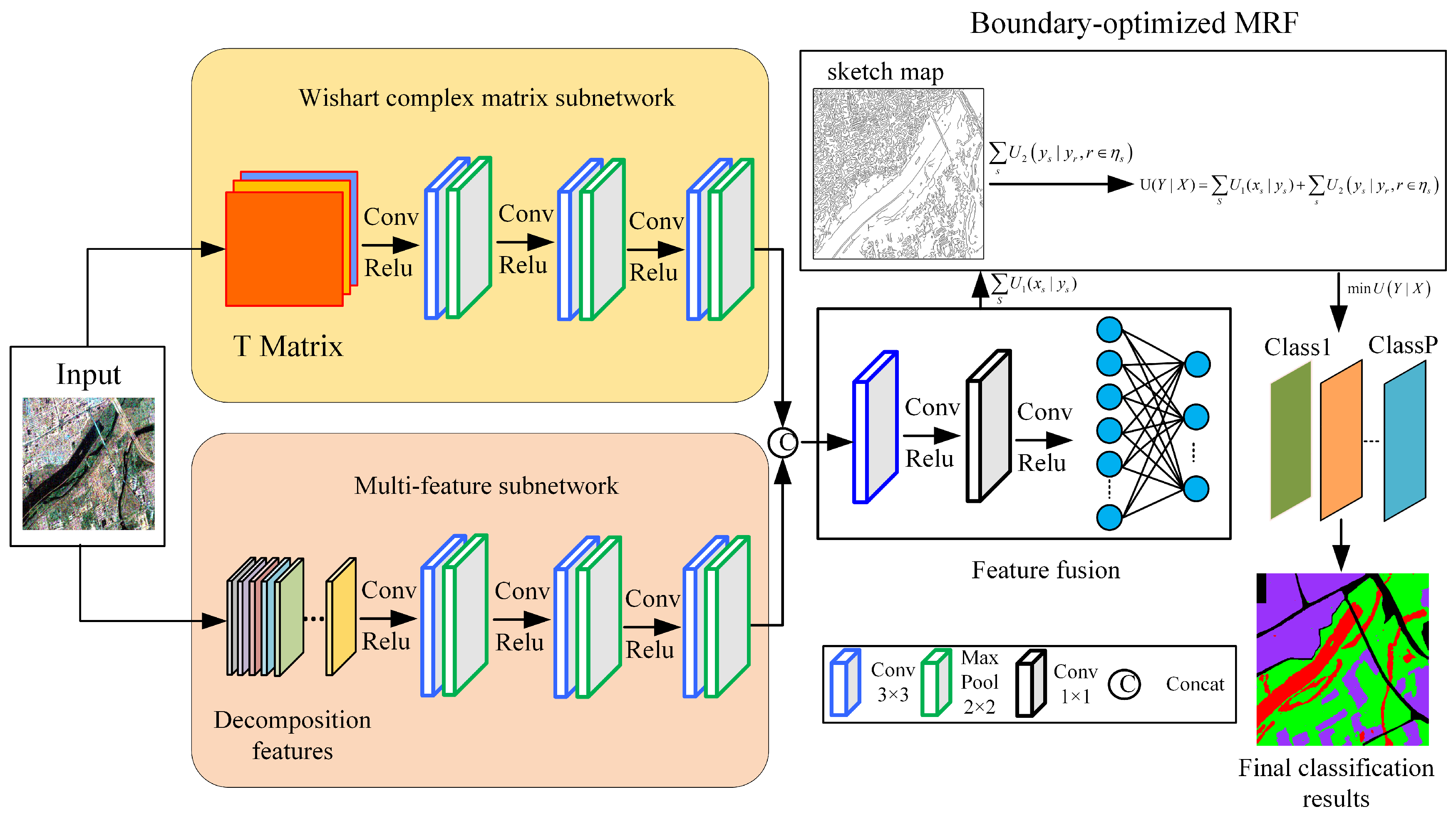
In this paper, a novel MRF-based double-channel convolution network (DCCNN-MRF) is proposed for PolSAR image classification, of which the framework is illustrated in
Figure 2. Firstly, a double-channel convolution network is developed to jointly learn the complex matrix and multiple features. On the one hand, a Wishart-based convolutional network is designed, which utilizes the complex matrix as the input, and defines the Wishart measurement as the first convolution layer. The Wishart convolution network effectively measures the similarity of complex matrices, followed by a CNN to learn deeper features. On the other hand, a multi-feature subnetwork is specifically designed to acquire various polarimetric scattering features. These features serve the purpose of providing supplementary information for the Wishart convolution network. Subsequently, a unified framework is developed to merge the outputs of the two subnetworks. To accomplish this fusion, multiple layer convolutions are employed to effectively combine the two types of features. Secondly, to suppress speckle and revise the edges, a MRF model is incorporated with the DCCNN network. This integration can also improve the overall performance of image classification. The data term in MRF model is defined as the class probability obtained from the DCCNN model, and the prior term is designed using an edge penalty function. The purpose of this edge penalty function is to reduce the confusion related to edges that may arise due to the high-level features of the deep model.
3.1. Double-channel convolution network
In this paper, a double-channel convolution network (DCCNN) is developed to jointly learn the complex matrix and various scattering features from PolSAR data, as shown in
Figure 2. The DCCNN network consists of two subnetworks: Wishart-based complex matrix and multi-feature subnetworks, which can learn complex matrix relationships and various polarimetric features, respectively. Then, an unified feature fusion module is designed to combine different features dynamically for enhancing the classification performance. This method provides a unified framework for integrating complex matrix and multi-feature learning. The incorporation of complementary information further enhances the classification performance.
1) Wishart-based complex matrix subnetwork
Traditional deep learning methods commonly convert the polarimetric complex matrix into a column vector. However, this conversion process results in the loss of both the matrix structure and data distribution of PolSAR data. In order to capture the characteristics of the complex matrix effectively, a Wishart-based complex matrix network is designed. This network aims to learn the statistical distribution of PolSAR complex matrix. The first layer in the neural network architecture is the Wishart convolution layer. This layer is responsible for converting the Wishart metric into a linear transformation, which corresponds to the convolution operation. To be specific, the coherency matrix
T, which is widely known to follow the Wishart distribution, is processed by this layer. For example, the distance between the
jth pixel
and the
ith class center
can be measured by the Wishart distance, defined as
where
is the log operation.
is the the trace operation of a matrix.
is the determinant operation of a matrix. However, the Wishart metric is not directly applicable to the convolution network due to its reliance on complex matrices. In [
25], Jiao et al. proposed a method to convert the Wishart distance into a linear operation. Firstly, the T matrix is converted into a vector as follows
where
and
are used to extract the real and imagery parts of a complex number respectively. This allows for the conversion of a complex matrix into a real-valued vector, where each element is a real value. Then, the Wishart convolution can be defined as
where
is the convolution kernel, and
is the
ith pixel value.
b is the bias vector defined as
.
is the output of Wishart convolution layer. Although it is a linear operation on vector
, it is equal to the Wishart distance between pixel
and class center
W.
In addition, to learn the statistical characteristics of complex matrices, we initialize the convolution kernel as the class center. Thus, the Wishart convolution is interpretable, which can learn the distance between each pixel and the class centers. By doing so, it overcomes the non-interpretability of traditional networks. The number of kernel is set equal to the number of classes, and the initial convolution kernel is calculated by averaging complex matrices of labeled samples for each class. After the first Wishart convolution layer, a complex matrix is transformed into a real value for each pixel. Subsequently, several CNN convolution layers are utilized to learn the contextual high-level features.
2) multi-feature subnetwork
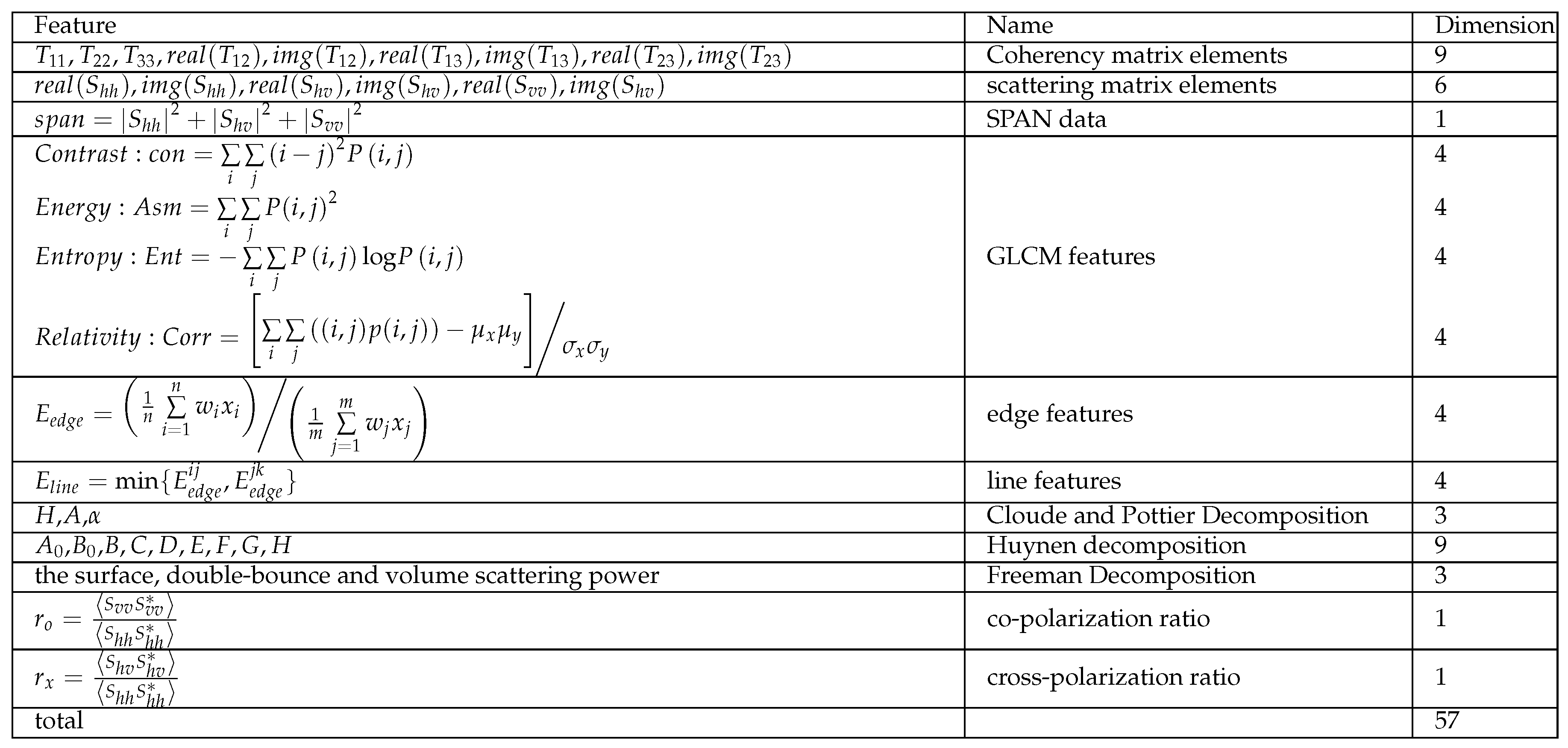
The Wishart subnetwork is capable of effectively learning the statistical characteristic of complex matrix. However, when it comes to heterogeneous areas, the individual complex matrices cannot learn the high-level semantic features. It’s because the heterogeneous structure results in neighboring pixels having significantly different scattering matrices, even though they belong to the same class. To learn high-level semantic in heterogeneous areas, it is necessary to employ multiple features that offer complementary information to the original data. In this paper, 57-dimension features are extracted, containing both the original data and various polarimetric decomposition-based features. These features include Cloude decomposition, Freeman decomposition, Yamaguki decomposition, and others. The detailed feature extraction can be found in Ref. [
40] as shown in
Table 1. The feature vector is defined as
, which describes each pixel from several aspects. Due to greatly various ranges of different features, the normalization process is employed initially. Subsequently, several layers of convolutions are applied to facilitate the learning of high-level features.
In addition, the network structure is designed as follows. a three-layer convolution is utilized to achieve multi-scale feature learning. The convolution kernel size is , and the moving step size is set to 1. Besides, the maximum pooling is selected to conduct the down-sampling, which effectively reduces both parameters and computational complexity while maintaining the same receptive field.
3) The proposed DCCNN fusion network
To enhance the benefits derived from both complex matrix and multiple features, a unified framework is designed to fuse these two subnetworks. To be specific, the complex matrix features
is extracted from Wishart subnetwork and the multi-feature vector
is achieved from the multi-feature subnetwork. Then, they are connected to construct the combined feature X. Later, several CNN convolution layers are utilized to fuse them. By multiple layer convolution, all the features are fused to capture global feature information effectively. After fully connected layer, discriminating features are extracted and useless features are suppressed. The classification accuracy of the target object can be improved by focusing on useful features. Therefore, the feature transformation of the proposed DCCNN network can be described as
where
means the extracted feature
from the Wishart subnetwork based on T matrix,
means the extracted feature
from the multi-feature subnetwork based on multi-feature
F. ⊕ is the connection operation of
and
. That is, features from two networks are connected, and then, the DCCNN network is utilized to generate the high-level feature
.Finally, the softmax layer is utilized for classification.
3.2. Combining edge-preserving MRF and DCCNN model
The proposed DCCNN model can effectively learn both the statistical characteristics and multiple features for PolSAR data. The learned high-level semantic features can improve the classification performance especially for heterogeneous areas. However, it contains a larger-scale contextual information with the increasing number of convolution layers, which is unfavourable for edge pixels, since the high-level features are difficult to identify neighboring pixels crossing the edge with different classes. So, the deep learning methods always blur edge details with high-level features. In order to learn the contextual relationships for heterogeneous terrain object and identify edge features accurately simultaneously, we combines the proposed DCCNN network with MRF to optimize the pixel level classification results.
Markov random field (MRF) is a widely used probability model which can learn contextual relationship by designing the energy function. The MRF can learn the pixel feature effectively, as well as incorporating the contextual information. In this paper, we design an edge penalty function to revise the edge pixels and suppress the speckle. In MRF, an energy function is defined, which consists of data and prior terms. The data term represents the probability of each pixel belonging to a certain class, while the prior term is the class prior probability. The energy function is defined as
where
is the data term, which stands for the probability of data
belonging to class
for pixel
s. In this paper, we define the data term as the probability learned from the DCCNN model.
is the prior term, which is the prior probability of class
. In MRF, the spatial contextual relationship is involved to learn the prior probability.
is neighboring set of pixel
s, and
r is the neighboring pixel of
s. When neighboring pixel
r has the same class label as pixel
s, the probability increases, otherwise decreases. When none of the neighboring pixels belong to class
, it indicates that pixel
s may likely be a noisy point. In such cases, it is advisable to revise the classification of pixel
s to match the majority class of its neighboring pixels. In addition,the neighborhood set is essential for the prior term. If pixel
s belongs to non-edge regions, a
square neighbor is suitable for suppressing speckle noises. If pixel
s is nearing the edges, its neighbors should be pixels along the edges instead of pixels in a square box. Furthermore, it’s not fair that all the neighbors contribute to the pixel with the same probability especially for edge pixels. Pixels in the same side of the edge are similar to the central pixel, which should have higher probability than totally different ones crossing the edge, even though they are also close to the central pixel. Neighboring pixels crossing the edge with a completely different class are unfavorable for estimating the probability of pixel
s, and can even lead to erroneous estimation.
In this paper, we firstly define the edge and non-edge regions for a PoLSAR image by utilizing the polarimetric sketch map [
39]. Firstly, the polarimetric sketch map is calculated by polarimetric edge detection and sketch pursuit methods. For each sketch segment, there are direction and length to characterize it. Then, edge regions are extracted by using a geometric structure block to expand a certain width along the sketch segments, such as five-pixel width.
Figure 3 illustrates an example of edge and non-edge regions.
Figure 3(a) is the PolSAR PauliRGB images.
Figure 3(b) are the extracted polarimetric sketch map from (a).
Figure 3(c) shows the geometric structure block. By expanding the sketch segments with (c), the edge and non-edge regions are shown in
Figure 3(d). Pixels in white are edge regions, while pixels in black are non-edge regions. For edge pixels, their directions are assigned as the direction of sketch segments.
In addition, we designed the adaptive neighborhood sets for edge and non-edge regions respectively. For non-edge regions, a
box is utilized as the neighbors. For edge regions, adaptive weighted neighborhood window is adopted to obtain the adaptive neighbors. That is, pixels along the edges have higher probability than other pixels. The weight of pixel
r to central pixel
s is measured by the revised Wishart distance, defined as
where
and
are the covariance matrices of neighboring and central pixels respectively. According to Wishart measurement, the weight of neighboring pixel
r to central pixel
s is defined as
The adaptive weighted neighboring window is shown in
Figure 4.
Figure 4(a) is the PauliRGB subimage of Xi’an area, in which pixel A is in the non-edge region, while pixels B and C belong to edge regions.
Figure 4(b) is the class label map of (a). We select
neighborhood window for pixel A in non-edge region as shown in
Figures 4(c).
Figure 4(d) and (e) are the adaptive weighted neighbors for point B and C respectively. In addition, for edge pixels, varying weights are assigned to the neighboring pixels. It is evident that the neighborhood pixels are always located along the edges. The black pixels that are distant from the center pixel no longer qualify as neighborhood pixels. Furthermore, neighborhood pixels with lighter colors are assigned higher weights, while pixels with darker colors have lower weights. From
Figures 4(c) and (d), we can see that pixels in the same side of edge have higher weights than ones in the other side, which can avoid the confusion by the neighboring pixels crossing the edge.
According to the adaptive weighted neighborhood, we develop an edge-preserved prior term that effectively integrates the contextual relationship while simultaneously minimizing the impact of neighboring pixels that traverse the edge. The prior term is built as
where
is the balance factor between data and prior terms.
and
are the class labels of pixel s and r respectively.
is the neighborhood weight of pixel
r to central pixel
s.
is the Kronecker delta function, defined as:
where
takes 1 when
and
are equal, otherwise 0. It is used to describe class relationship between the central point and its neighbor pixels.
After MRF optimization, the proposed method can obtain the final classification map with both better region homogeneity in heterogeneous regions and edge preservation. The proposed DCCNN-MRF algorithm procedure is given in
Algorithm 1.
|
Algorithm 1 Algorithm procedure of the proposed DCCNN-MRF method |
|
Input: PolSAR coherency matrix T, PolSAR multiple features F, class label map . Balance factor and class number C
|
|
Step 1: Extract multiple of scattering features F from PolSAR images by Table 1. |
|
Step 2: Learn the complex matrix features from original data T by the Wishart subnetwork. |
|
Step 3: Learn the high-level features from multiple features F by the multi-feature subnetwork. |
|
Step 4: Combine the and into the DCCNN model, and learn the fused feature . |
|
Step 5: Obtain the class probability P and estimated class label map Y by the DCCNN model. |
|
Step 6: Obtain the sketch map of the PolSAR image, and compute the adaptive weighted neighbors for edge pixels by Equation (8). |
|
Step 7:Optimize the estimated class label Y using Equation (6) by the edge-preserved MRF model. |
|
Output: class label estimation map Y. |
Figure 1.
Examples of polarimetric sketch maps. (a) PauliRGB PolSAR image on Xi’an data set; (b) PauliRGB PolSAR image on Flevoland data set; (c) Corresponding polarimetric sketch map on Xi’an data set; (d) Corresponding polarimetric sketch map on Flevoland data set.
Figure 1.
Examples of polarimetric sketch maps. (a) PauliRGB PolSAR image on Xi’an data set; (b) PauliRGB PolSAR image on Flevoland data set; (c) Corresponding polarimetric sketch map on Xi’an data set; (d) Corresponding polarimetric sketch map on Flevoland data set.
Figure 2.
Framework of the proposed double-channel CNN and MRF model for PolSAR image classification.
Figure 2.
Framework of the proposed double-channel CNN and MRF model for PolSAR image classification.
Figure 3.
Example of edge and non-edge regions. (a) PauliRGB image of Ottawa; (b) The corresponding polarimetric sketch map; (c) Geometric structural block; (d) The white area is edge regions and the black area is the non-edge regions.
Figure 3.
Example of edge and non-edge regions. (a) PauliRGB image of Ottawa; (b) The corresponding polarimetric sketch map; (c) Geometric structural block; (d) The white area is edge regions and the black area is the non-edge regions.
Figure 4.
Example of adaptive neighbor structures. (a) the PauliRGB image of Xi’an area, the point A is in the non-edge region, and point B and point C are in the edge region; (b) The label map of (a); (c) fixed neighborhood for point A; (d) weighted neighborhood structure for point B; (e)weighted neighborhood structure for point C.
Figure 5.
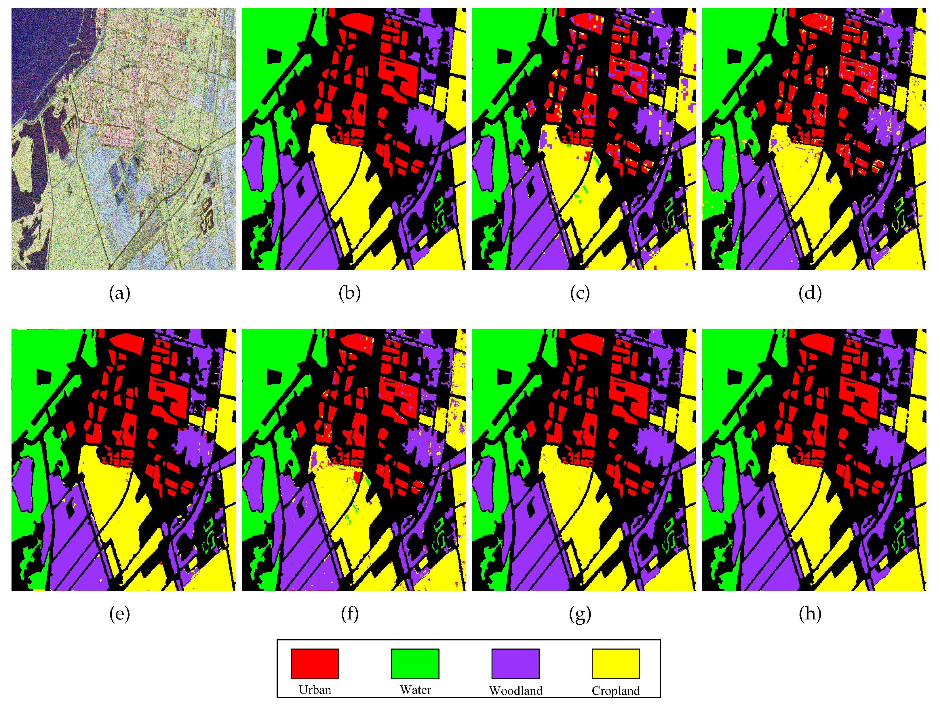
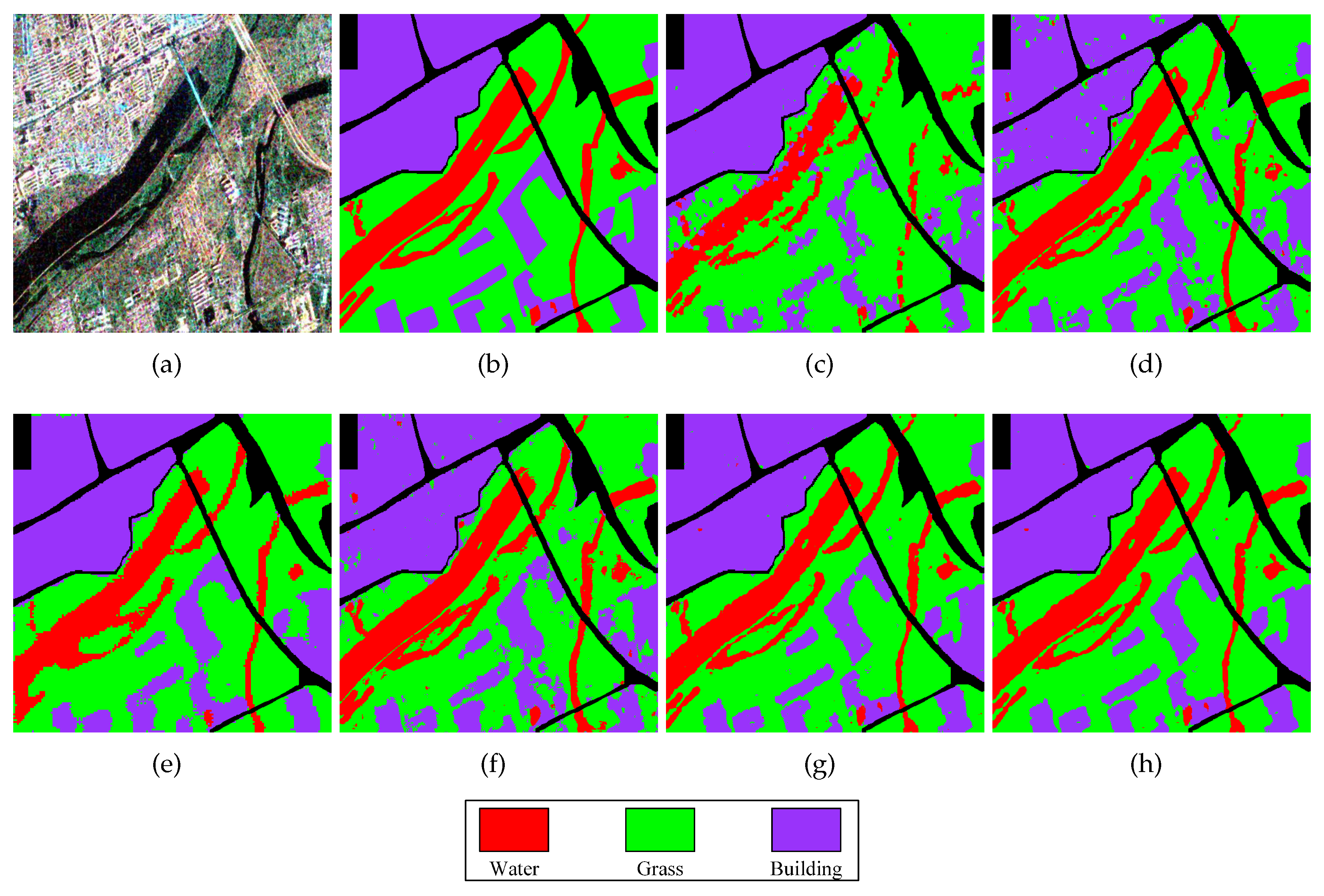
Classification results of different methods in the Xi’an area. (a) PauliRGB image of Xi’an area; (b) The label map of (a); (c) The classification map by the Super-RF method; (d) The classification map by the DBDA method; (e) The classification map by the S3ANet method; (f) The classification map by the CV-CNN method; (g)The classification map by the proposed DCCNN method; (h) The classification map by the proposed DCCNN-MRF method.
Figure 6.
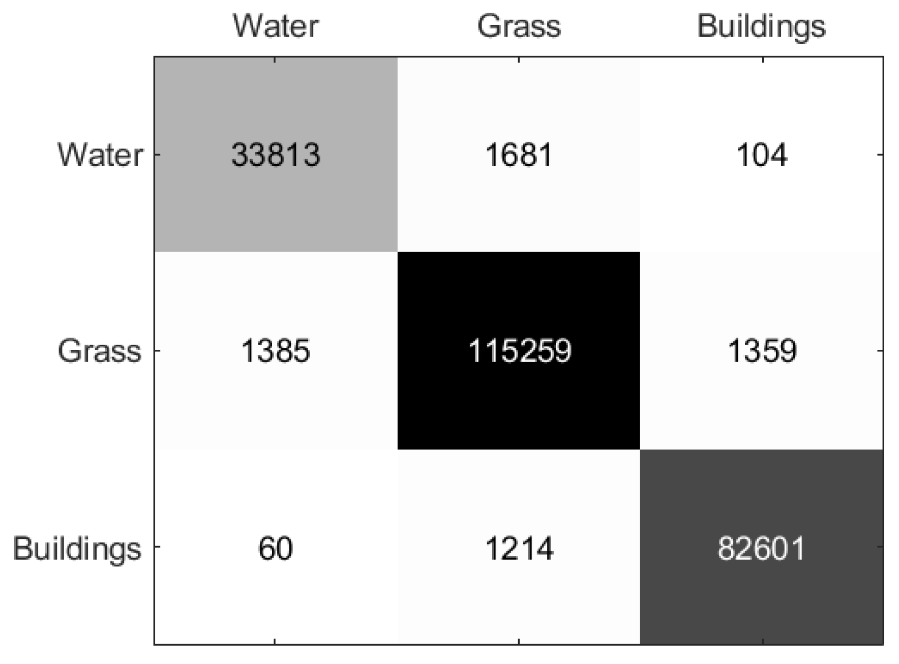
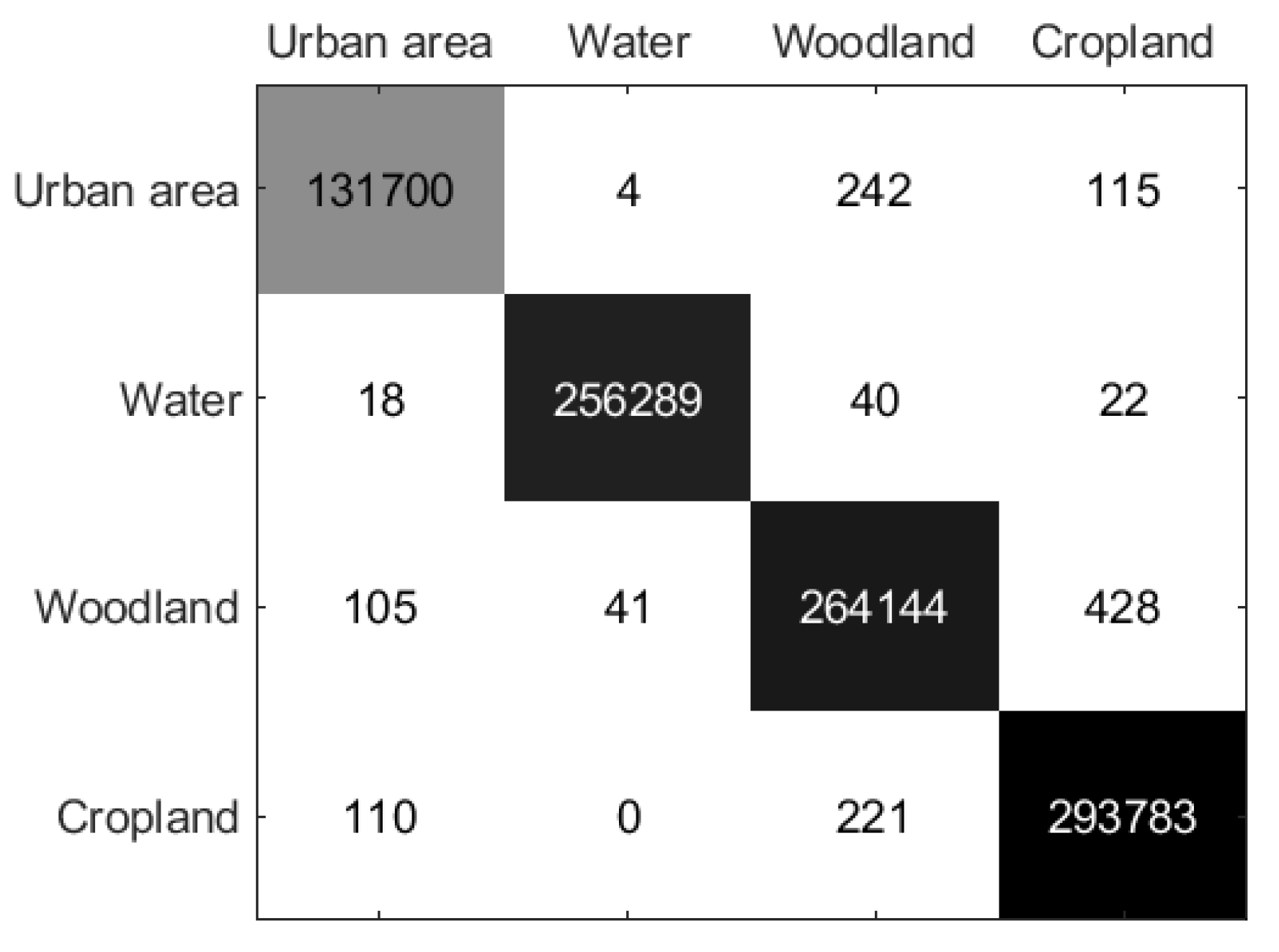
Confusion matrix of the proposed method on Xi’an Data Set.
Figure 6.
Confusion matrix of the proposed method on Xi’an Data Set.
Figure 8.
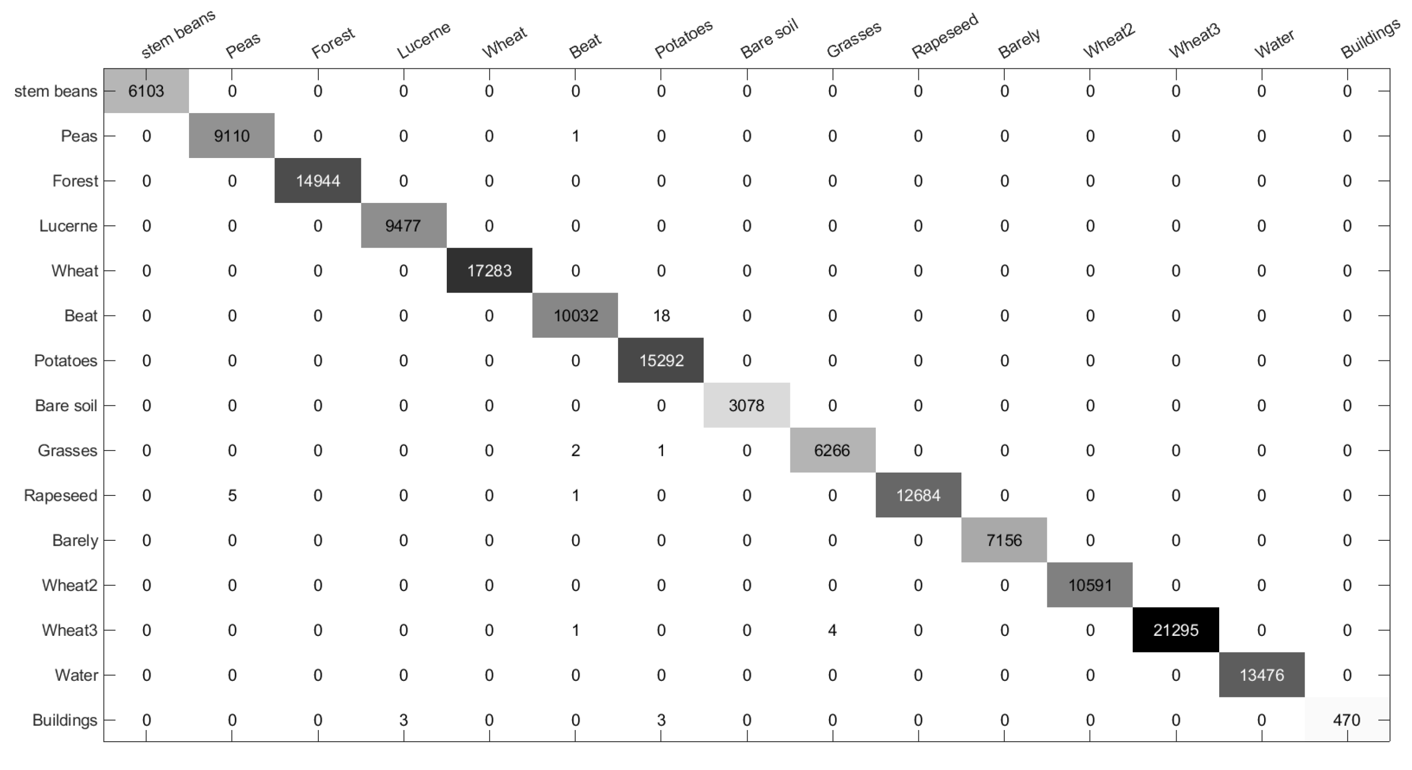
Confusion matrix of the proposed method on Flevoland 1 Data Set.
Figure 8.
Confusion matrix of the proposed method on Flevoland 1 Data Set.
Figure 10.
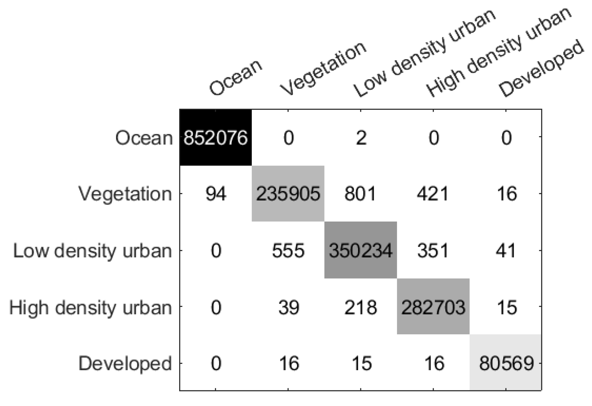
Confusion matrix of the proposed method on San Francisco Data Set.
Figure 10.
Confusion matrix of the proposed method on San Francisco Data Set.
Figure 12.
Confusion matrix of the proposed method on Flevoland 2 Data Set.
Figure 12.
Confusion matrix of the proposed method on Flevoland 2 Data Set.
Figure 13.
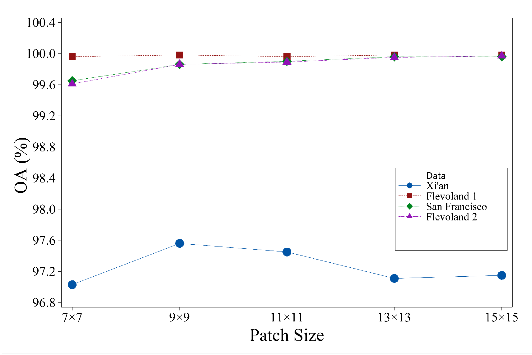
The effect of patch size on classification accuracy.
Figure 13.
The effect of patch size on classification accuracy.
Figure 14.
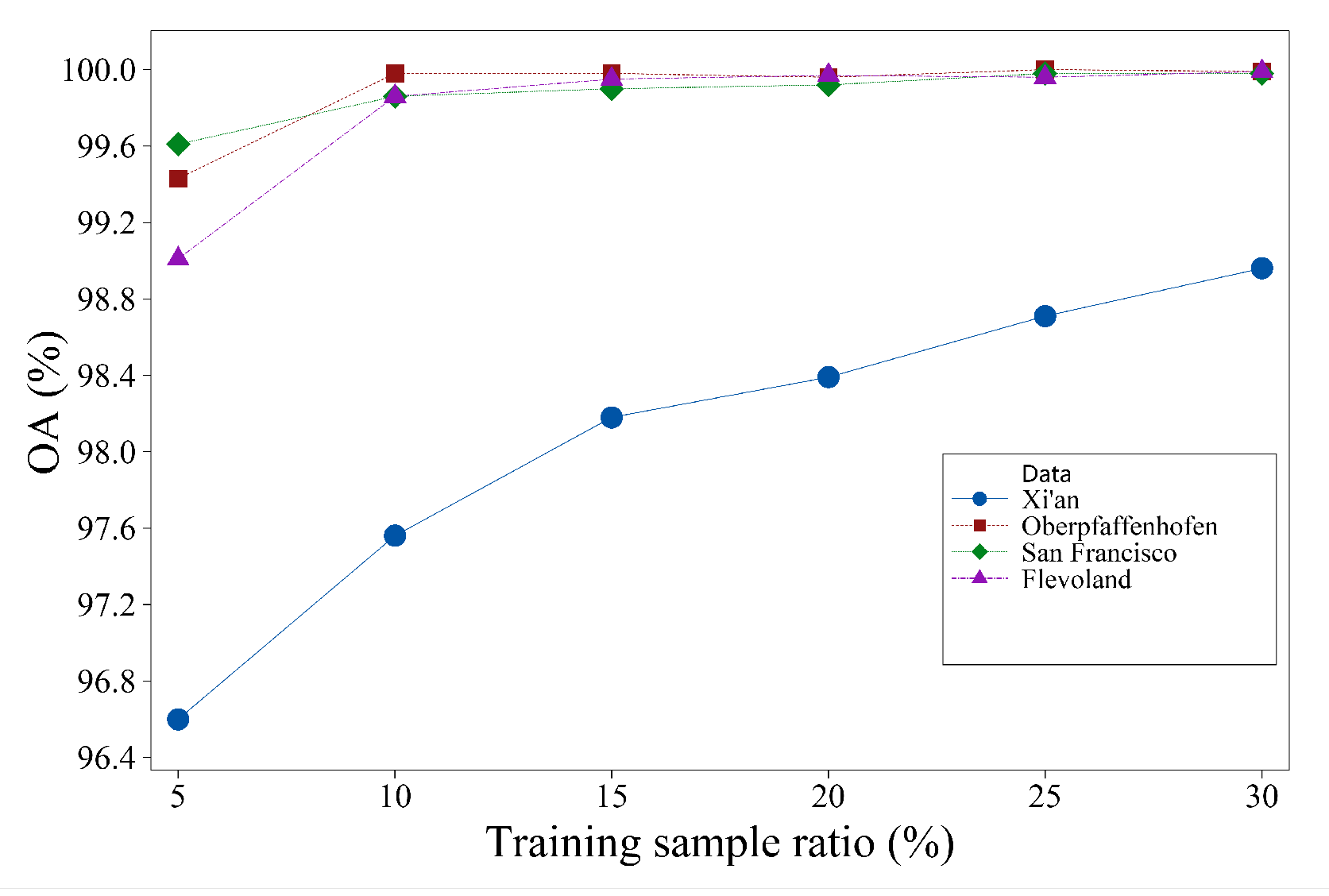
The effect of training sample ratio on classification accuracy.
Figure 14.
The effect of training sample ratio on classification accuracy.
Table 1.
Multiple Feature Extraction of PolSAR images.
Table 1.
Multiple Feature Extraction of PolSAR images.
Table 2.
PolSAR data set used within the experiments.
Table 2.
PolSAR data set used within the experiments.
| Name |
System |
Band |
Dimensions |
Resolution |
Class |
| Xi’an |
RADARSAT-2 |
C |
m |
|
3 |
| Flevoland1 |
AIRSAR |
L |
m |
|
15 |
| San Francisco |
RADARSAT-2 |
C |
m |
|
5 |
| Flevoland2 |
AIRSAR |
C |
m |
|
4 |
Table 3.
Classification accuracy of different methods on Xi’an Data Set. (%)
Table 3.
Classification accuracy of different methods on Xi’an Data Set. (%)
| class |
Super-RF |
DBDA |
S3ANet |
CV-CNN |
DCCNN |
DCCNN-MRF |
| water |
70.91 |
89.88 |
84.39 |
95.30 |
94.88 |
94.99 |
| grass |
94.97 |
93.13 |
93.99 |
88.25 |
97.49 |
97.67 |
| building |
90.94 |
91.56 |
96.72 |
95.34 |
98.31 |
98.48 |
| OA |
89.94 |
92.09 |
93.51 |
91.81 |
97.39 |
97.56 |
| AA |
85.61 |
91.53 |
91.70 |
92.96 |
96.90 |
97.05 |
| Kappa |
83.02 |
86.91 |
89.24 |
86.67 |
95.69 |
95.96 |
Table 4.
Classification accuracy of different methods on Flevoland 1 Data Set (%).
Table 4.
Classification accuracy of different methods on Flevoland 1 Data Set (%).
| class |
Super-RF |
DBDA |
S3ANet |
CV-CNN |
DCCNN |
DCCNN-MRF |
| stembeans |
96.77 |
99.97 |
93.79 |
99.72 |
100 |
100 |
| peas |
98.64 |
99.53 |
96.63 |
99.99 |
99.98 |
99.99 |
| forest |
95.88 |
99.37 |
96.01 |
99.82 |
100 |
100 |
| lucerne |
96.63 |
100 |
96.86 |
98.17 |
99.97 |
100 |
| wheat |
99.05 |
98.69 |
99.86 |
98.66 |
100 |
100 |
| beat |
95.70 |
99.83 |
98.09 |
99.22 |
99.82 |
99.82 |
| potatoes |
96.04 |
99.59 |
95.21 |
99.14 |
100 |
100 |
| baresoil |
94.57 |
83.11 |
100 |
100 |
100 |
100 |
| grasses |
84.03 |
85.12 |
68.19 |
99.94 |
99.94 |
99.95 |
| rapeseed |
53.13 |
65.23 |
81.60 |
94.18 |
99.94 |
99.95 |
| barely |
100 |
85.52 |
95.11 |
99.58 |
100 |
100 |
| wheat2 |
79.93 |
99.48 |
96.83 |
99.41 |
100 |
100 |
| wheat3 |
99.39 |
99.23 |
99.79 |
99.37 |
99.97 |
99.98 |
| water |
100 |
89.93 |
99.27 |
99.99 |
100 |
100 |
| building |
0 |
95.17 |
66.39 |
100 |
98.95 |
98.74 |
| OA |
92.18 |
94.31 |
95.01 |
98.96 |
99.97 |
99.98 |
| AA |
85.98 |
93.32 |
92.24 |
99.15 |
99.90 |
99.90 |
| Kappa |
91.44 |
93.79 |
94.55 |
98.87 |
99.97 |
99.97 |
Table 5.
Classification accuracy of different methods on San Francisco Data Set (%).
Table 5.
Classification accuracy of different methods on San Francisco Data Set (%).
| class |
Super-RF |
DBDA |
S3ANet |
CV-CNN |
DCCNN |
DCCNN-MRF |
| ocean |
99.98 |
99.32 |
99.73 |
99.99 |
100 |
100 |
| vegetation |
93.89 |
88.20 |
97.40 |
96.42 |
99.31 |
99.44 |
| low-density urban |
97.31 |
98.33 |
98.27 |
94.51 |
99.51 |
99.73 |
| high-density urban |
77.76 |
90.00 |
99.82 |
96.37 |
99.80 |
99.90 |
| develop |
81.00 |
81.15 |
99.47 |
95.92 |
99.87 |
99.94 |
| OA |
94.33 |
95.39 |
99.14 |
97.71 |
99.78 |
99.86 |
| AA |
89.99 |
91.40 |
98.93 |
96.64 |
99.70 |
99.80 |
| Kappa |
91.81 |
93.36 |
98.76 |
96.70 |
99.68 |
99.79 |
Table 6.
Classification accuracy of different methods on Flevoland 2 Data Set (%).
Table 6.
Classification accuracy of different methods on Flevoland 2 Data Set (%).
| class |
Super-RF |
DBDA |
S3ANet |
CV-CNN |
DCCNN |
DCCNN-MRF |
| urban |
81.84 |
89.37 |
99.91 |
96.26 |
99.57 |
99.73 |
| water |
98.69 |
95.83 |
98.86 |
99.85 |
99.96 |
99.97 |
| woodland |
94.92 |
95.82 |
97.11 |
96.48 |
99.70 |
99.78 |
| cropland |
94.16 |
97.69 |
99.17 |
93.94 |
99.78 |
99.89 |
| OA |
93.88 |
95.50 |
98.61 |
96.57 |
99.78 |
99.86 |
| AA |
92.40 |
94.68 |
98.76 |
96.63 |
99.76 |
99.84 |
| Kappa |
91.61 |
93.84 |
98.11 |
95.33 |
99.70 |
99.81 |
Table 7.
Classification accuracy of different subnetworks on four data sets (%).
Table 7.
Classification accuracy of different subnetworks on four data sets (%).
| Data set |
Xi’an |
Flevoland 1 |
San Francisco |
Flevoland 2 |
| Accuracy |
OA |
Kappa |
OA |
Kappa |
OA |
Kappa |
OA |
Kappa |
| Wishart |
88.58 |
81.12 |
95.49 |
95.08 |
92.36 |
89.00 |
94.37 |
92.31 |
| Multi-feature |
95.77 |
92.98 |
99.91 |
99.90 |
99.75 |
99.64 |
99.76 |
99.68 |
| DCCNN |
97.39 |
95.69 |
99.97 |
99.97 |
99.78 |
99.68 |
99.78 |
99.70 |
Table 8.
Classification accuracy of different model settings on data sets (%).
Table 8.
Classification accuracy of different model settings on data sets (%).
| Data set |
Xi’an |
Flevoland 1 |
San Francisco |
Flevoland 2 |
| Accuracy |
OA |
Kappa |
OA |
Kappa |
OA |
Kappa |
OA |
Kappa |
| Wishart |
88.58 |
81.12 |
95.49 |
95.08 |
92.36 |
89.00 |
94.37 |
92.31 |
| Wishart+MRF |
89.25 |
82.24 |
95.93 |
95.55 |
93.00 |
89.92 |
95.84 |
94.33 |
| Multi-feature |
95.77 |
92.98 |
99.91 |
99.90 |
99.75 |
99.64 |
99.76 |
99.68 |
| Multi-feature+MRF |
95.98 |
93.33 |
99.94 |
99.93 |
99.83 |
99.76 |
99.85 |
99.79 |
| DCCNN |
97.39 |
95.69 |
99.97 |
99.97 |
99.78 |
99.68 |
99.78 |
99.70 |
| DCCNN+MRF |
97.56 |
95.96 |
99.98 |
99.97 |
99.86 |
99.79 |
99.86 |
99.81 |
Table 9.
Running time of different methods on Xi’an data set (s).
Table 9.
Running time of different methods on Xi’an data set (s).
| |
Super-RF |
DBDA |
S3ANet |
CV-CNN |
DCCNN-MRF |
| training time |
59.22 |
239.35 |
461.33 |
7872.68 |
121.99 |
| test time |
1.85 |
32.50 |
1.43 |
19.88 |
13.24 |
