Submitted:
04 October 2023
Posted:
05 October 2023
You are already at the latest version
Abstract
Keywords:
1. Introduction
- A method to quantitatively analyze the relationship between the molecular structure of perfumes and human olfactory perception, advancing understanding in the field of scent psychophysics.
- Systematically extract and utilize consumer feedback from digital platforms, such as Parfumo, to inform the molecular design process, underscoring the importance of integrating market analysis in product design.
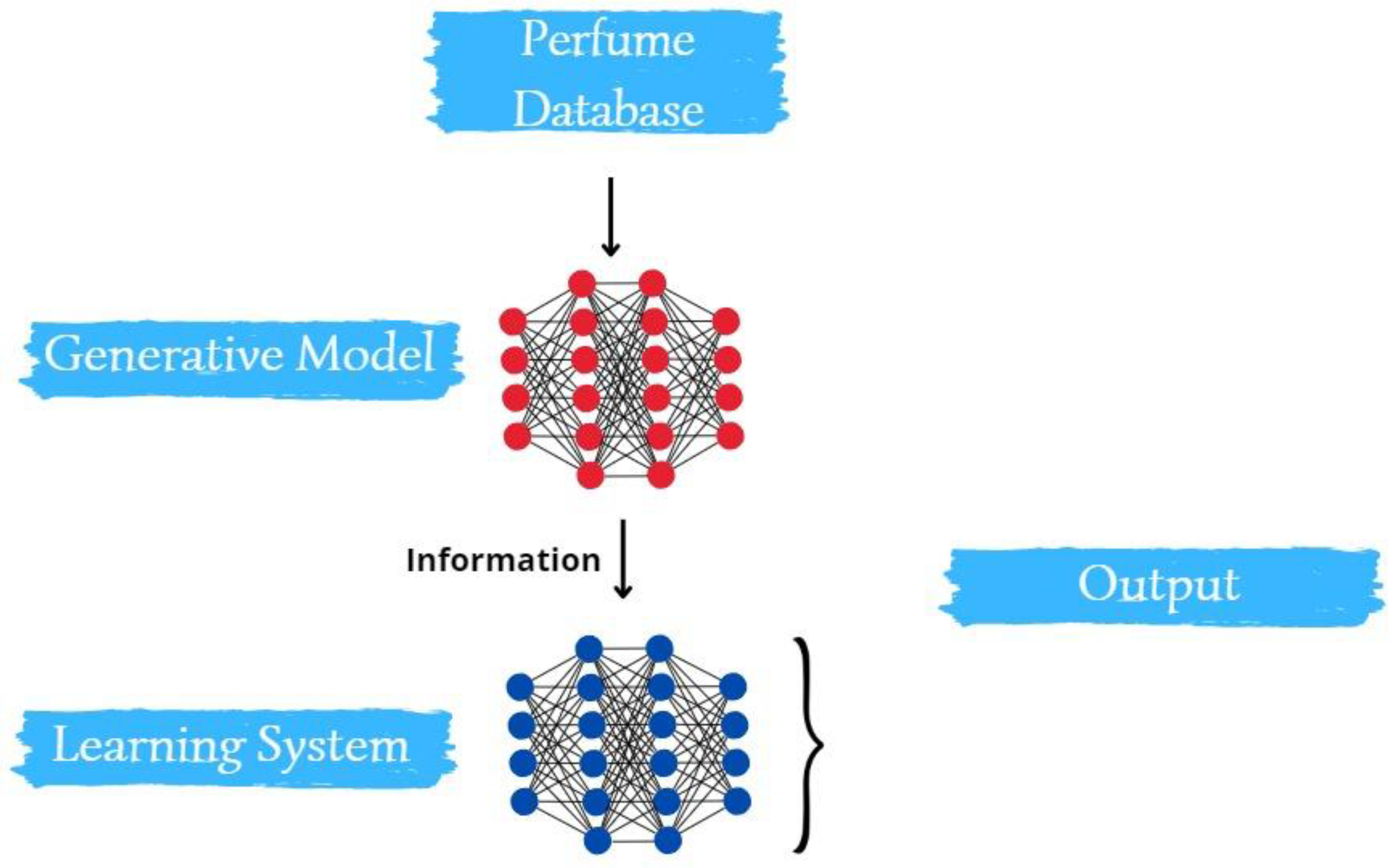
- Design and validate an AI-based molecule generator tailored for scent molecule prediction, a first in the domain of fragrance chemistry.
- The proposed AI approach to predict successful scent molecules based on consumer feedback, potentially reduces the lengthy and costly trial-and-error process traditionally associated with perfume creation.
- It is proposed an algorithmic model that incorporates real-world consumer feedback, thereby ensuring the synthesized molecules have a higher likelihood of market success.
2. Methodology
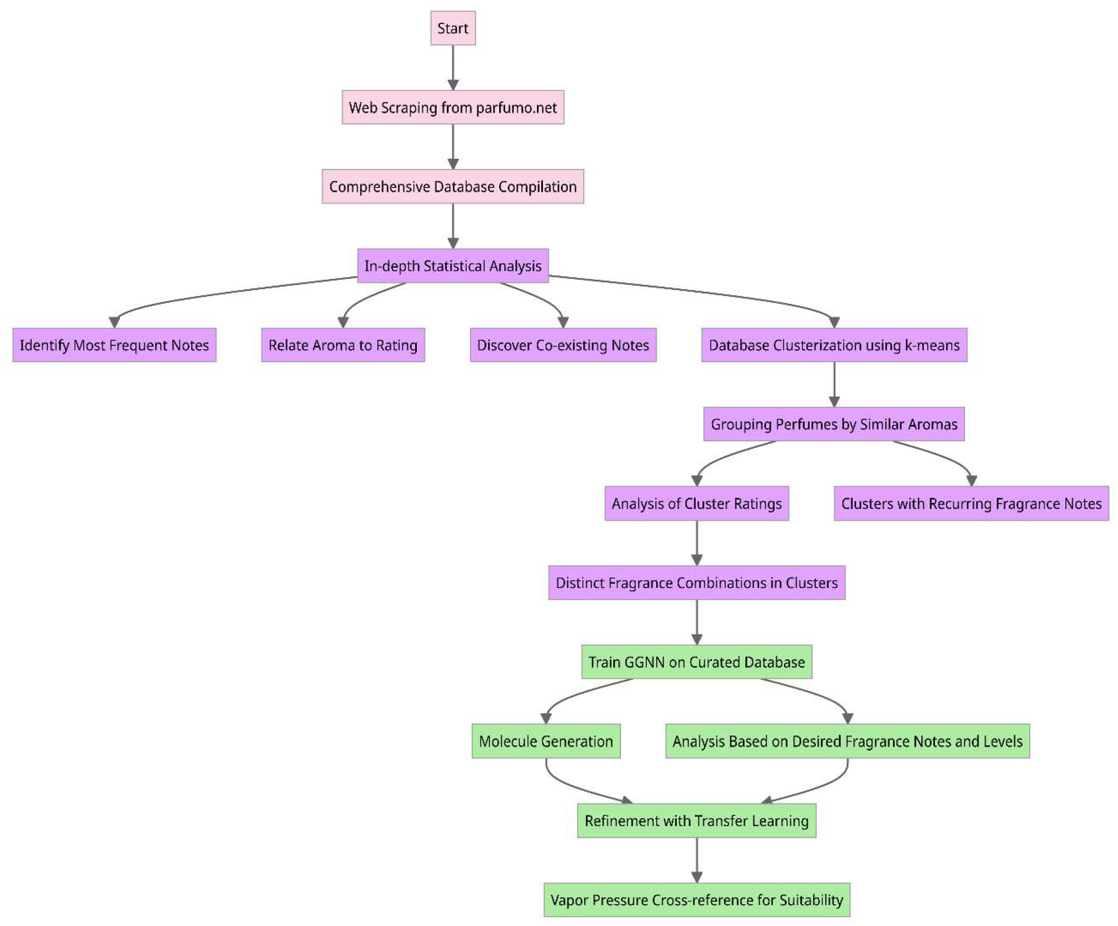
- Data Collection via Web Scraping: The first step in the proposed methodology involves developing a specialized web scraping program to collect data from the Parfumo forum. This data encompasses consumer feedback, fragrance notes, and ratings on many perfumes. By systematically extracting this information, compiling a comprehensive database serves as a cornerstone for the subsequent step in the methodology.
- In-depth Statistical Analysis: After amassing the database, an analytical phase is proposed to interrogate the data for meaningful patterns and insights. This step sought answers to questions pivotal to the proposed goals: Which fragrance notes appear most frequently across perfumes? Is there a correlation between certain aromatic notes and higher consumer ratings? Are there specific fragrance notes that are commonly paired together? Such queries enabled us to understand consumer preferences and market trends better.
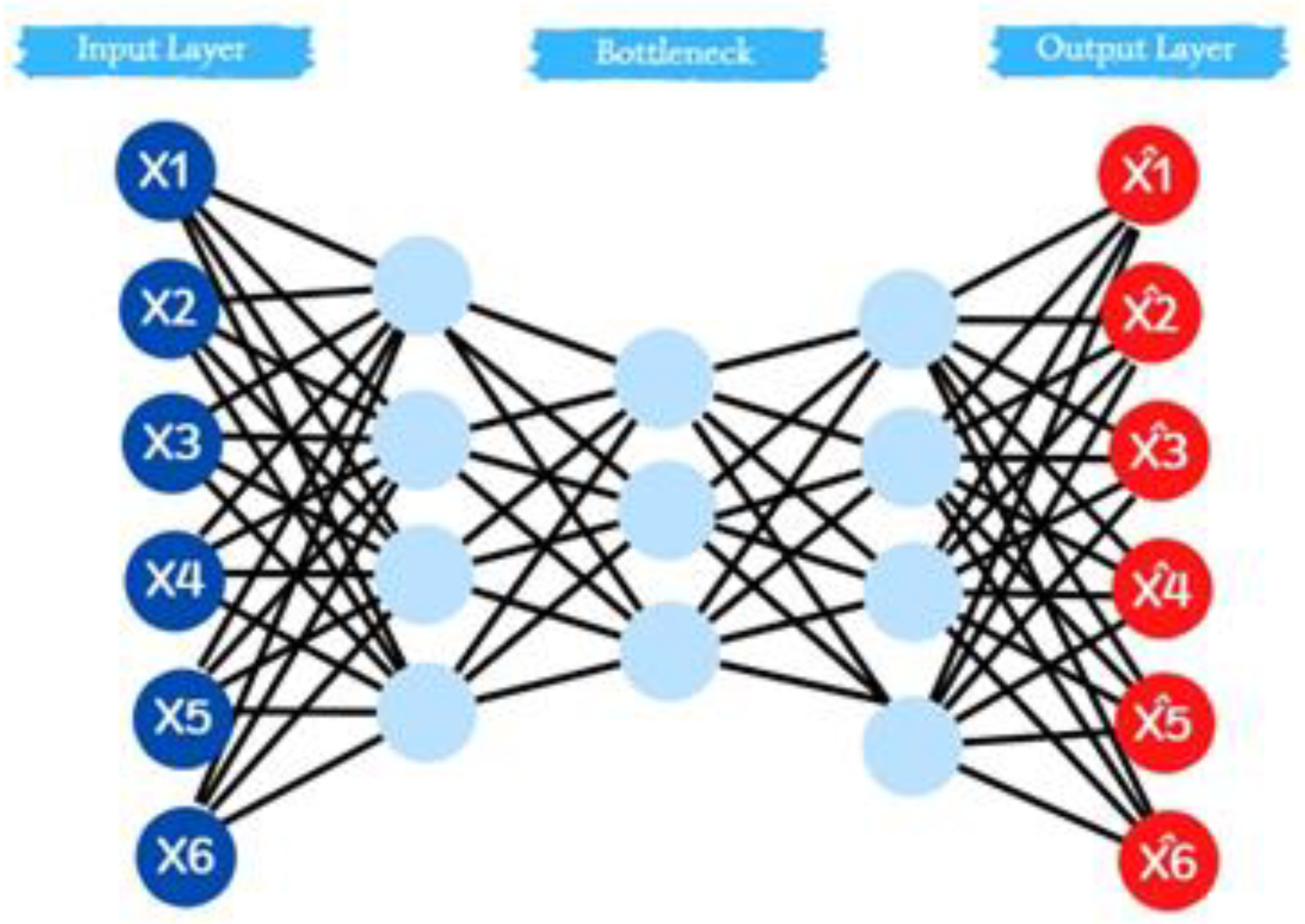
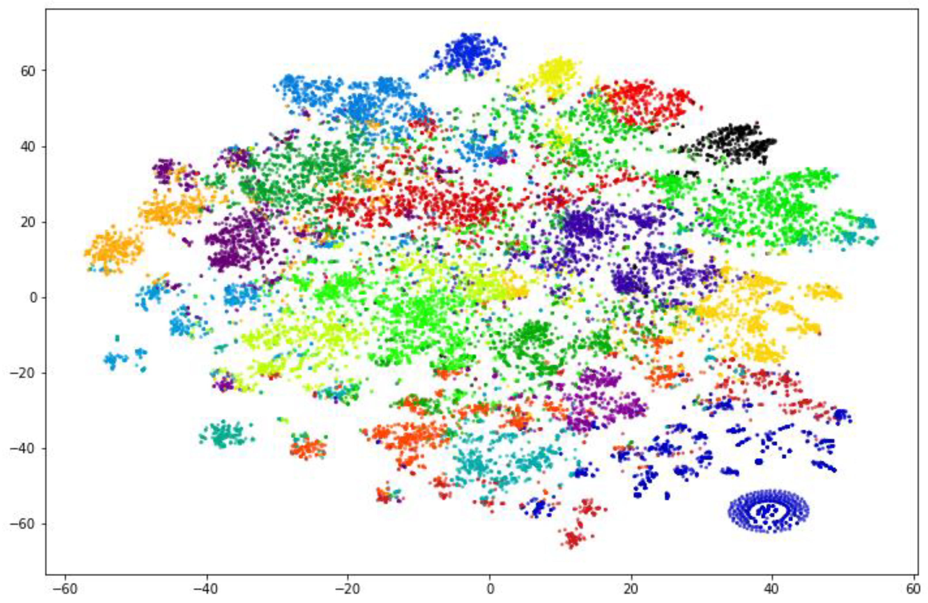
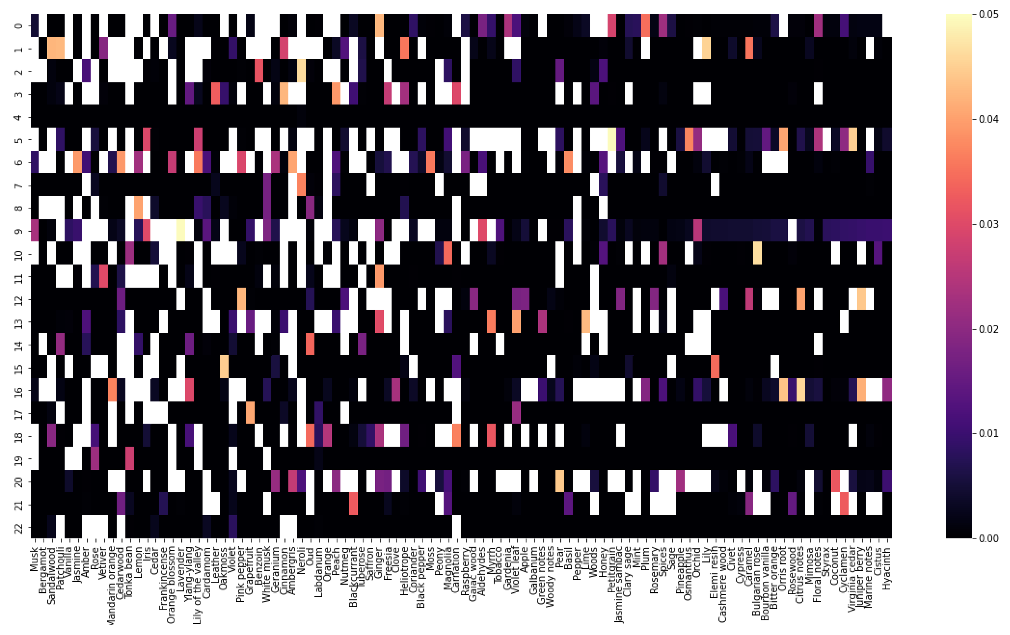
- Database Clustering using the k-means Algorithm: To delve deeper into the interplay of fragrance notes, it is proposed to employ the k-means clustering algorithm. This technique allowed us to group perfumes with similar aromatic profiles, particularly those with recurrent but uniquely combined fragrance notes. The outcome was a categorization of perfumes into distinct clusters, each signifying a particular scent profile.
- Evaluative Analysis of Cluster Ratings: With our clusters defined, the next step focuses on understanding how each cluster fared in consumer ratings. This step provides a granular view of the market reception for different aromatic combinations and provides the necessary information to the AI framework to prioritize which scent profiles resonate most with consumers.
-
Molecule Generation for Desired Perfume Profiles: Central to the proposed methodology is the aspiration to generate a roster of molecules that align with select perfume scents. This process was two-pronged:
- Training Phase: We trained a gated graph neural network (GGNN) on a curated database comprising known molecules and their associated fragrance notes.
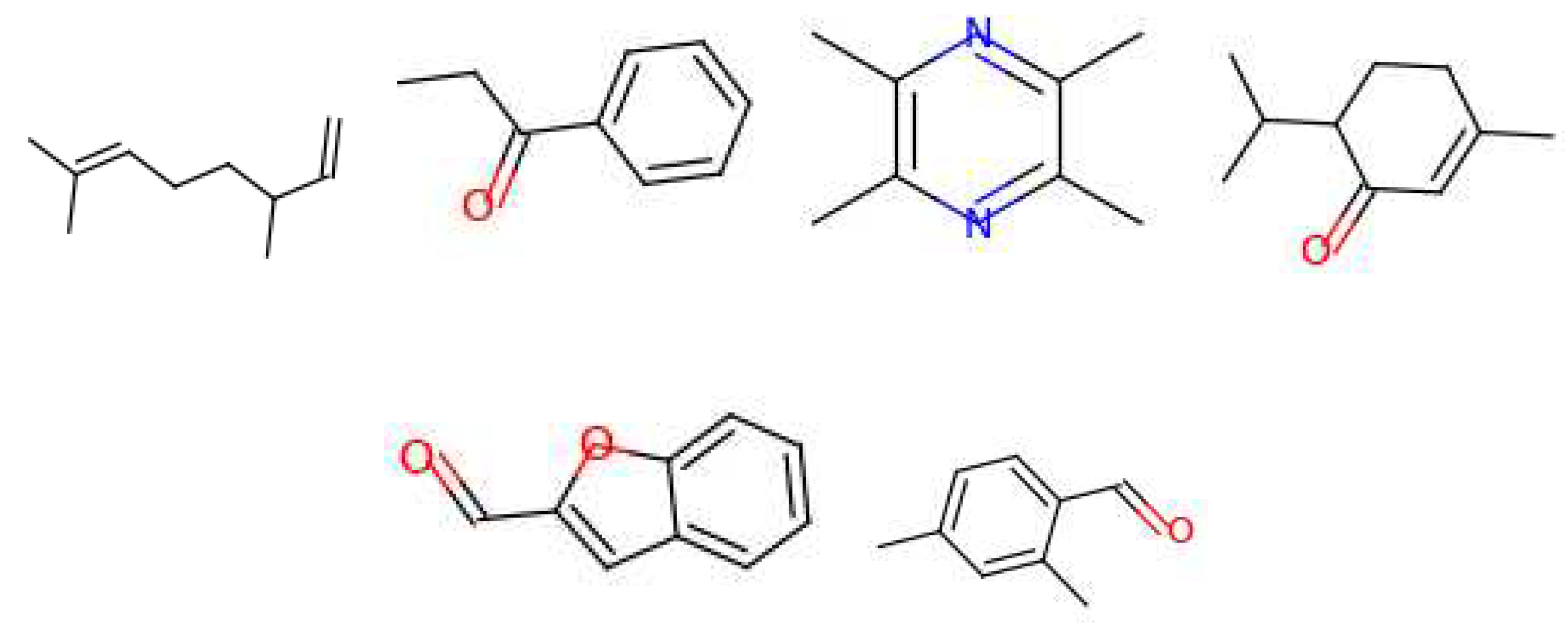
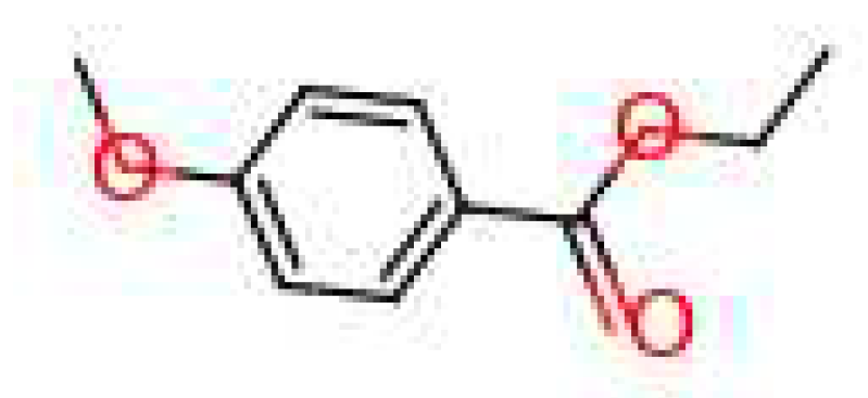
- Generation and Refinement: Leveraging the trained GGNN, we embarked on generating a diverse set of molecules. To fine-tune this generation process, we integrated transfer learning techniques, narrowing down to molecules that match our targeted scent profiles.
- VI.
- Assessment of Generated Molecules: Post-generation, an evaluation is proposed to ensure the suitability of the molecules. Hence, we propose cross-referencing the vapor pressure of each synthesized molecule against existing databases. This ensured that the generated molecules matched the aroma profile and conformed to the requisite intensity of the fragrance notes.
2.1. Data Collection via Web Scraping and In-Depth Statistical Analysis
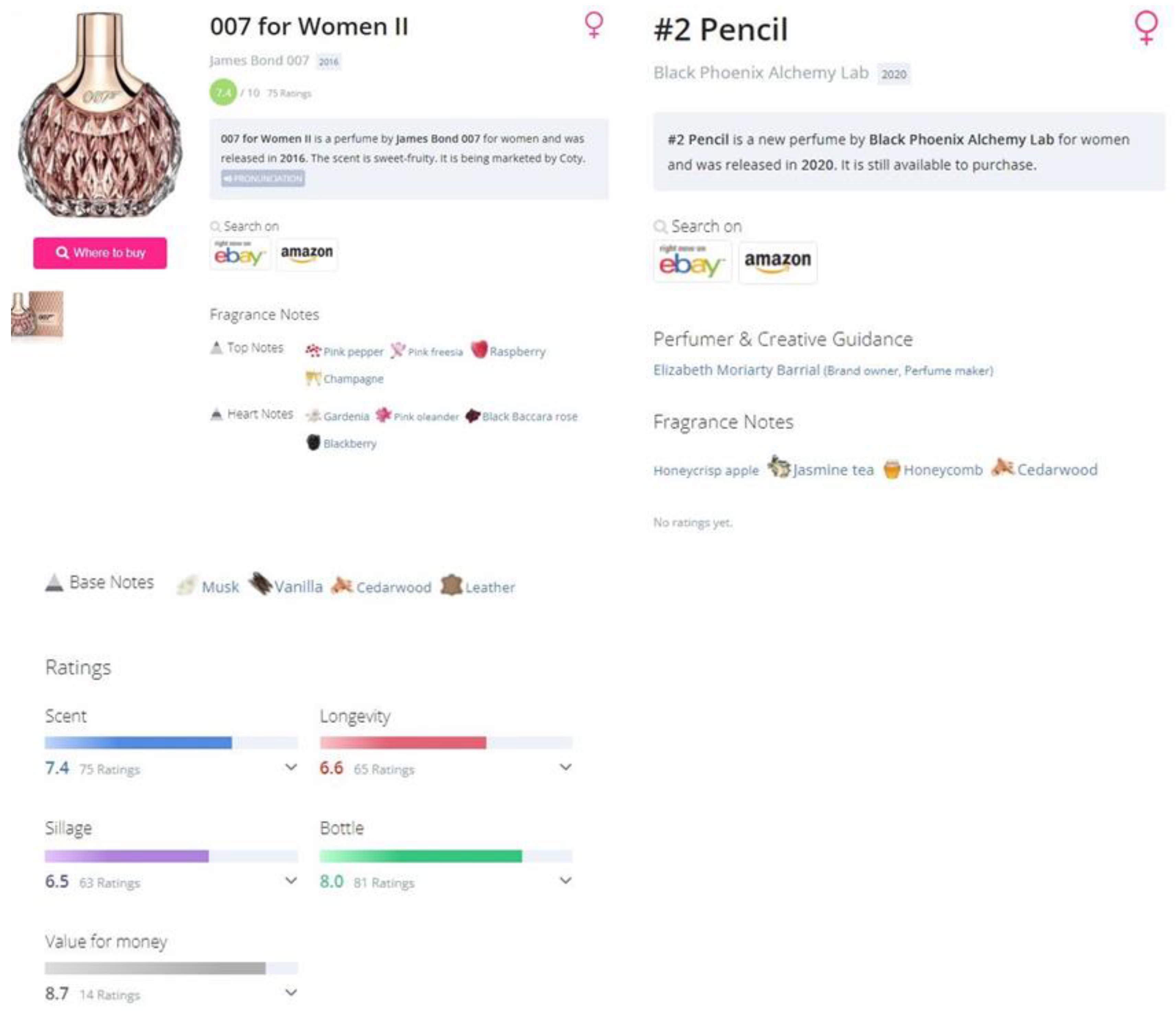
-
Which fragrance notes appear most frequently across perfumes?To answer this question, it is necessary to count how many perfumes contain a given fragrance note for every fragrance note that is available.
-
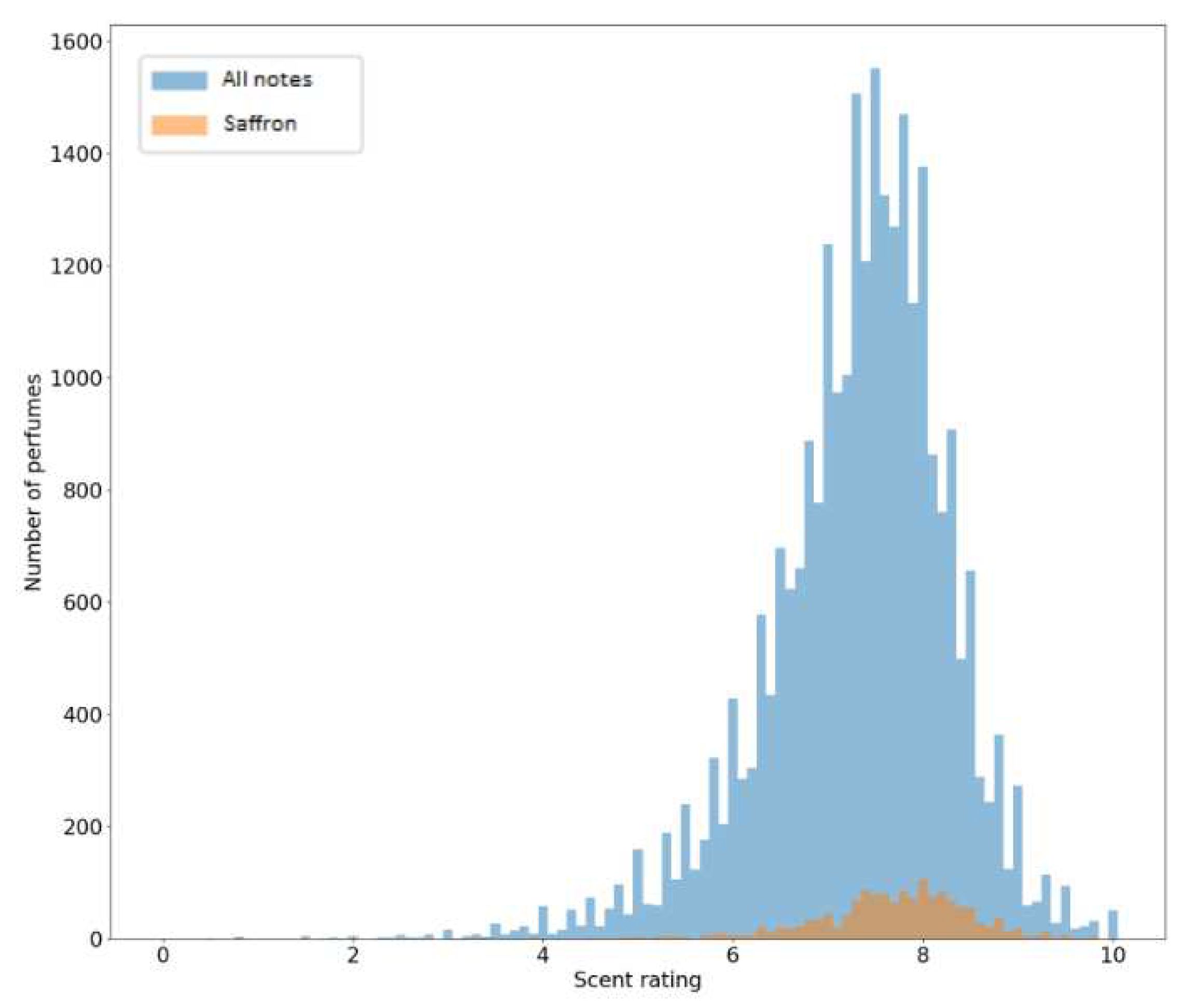
Is there a correlation between certain aromatic notes and higher consumer ratings?Here, it is necessary to consider all the perfumes that contain a given fragrance note and calculate the average of the ratings of all perfumes. It is also useful to calculate the sum of ratings for each fragrance note (Sum of the ratings of all the perfumes that contain a given note)
-
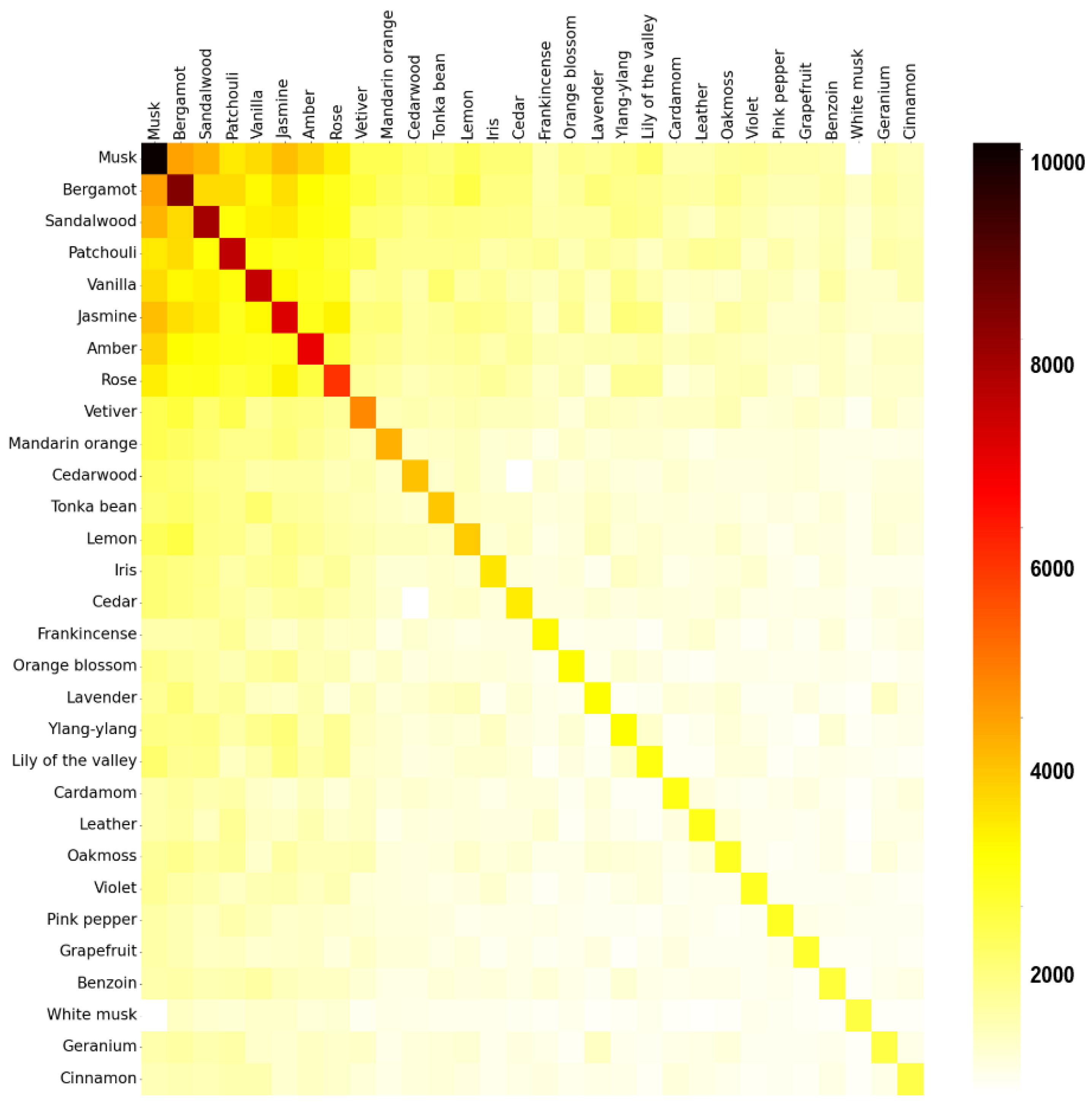
Are there specific fragrance notes that are commonly paired together?Firstly, a matrix is created using a technique called one-hot encoding. The matrix contains all the perfumes as rows and all the fragrance notes available as columns. If a perfume contains a given fragrance note, the value of the cell is one, else, it is zero. Next, a co-occurrence of fragrance notes matrix is calculated by multiplying the original matrix with its transpose.
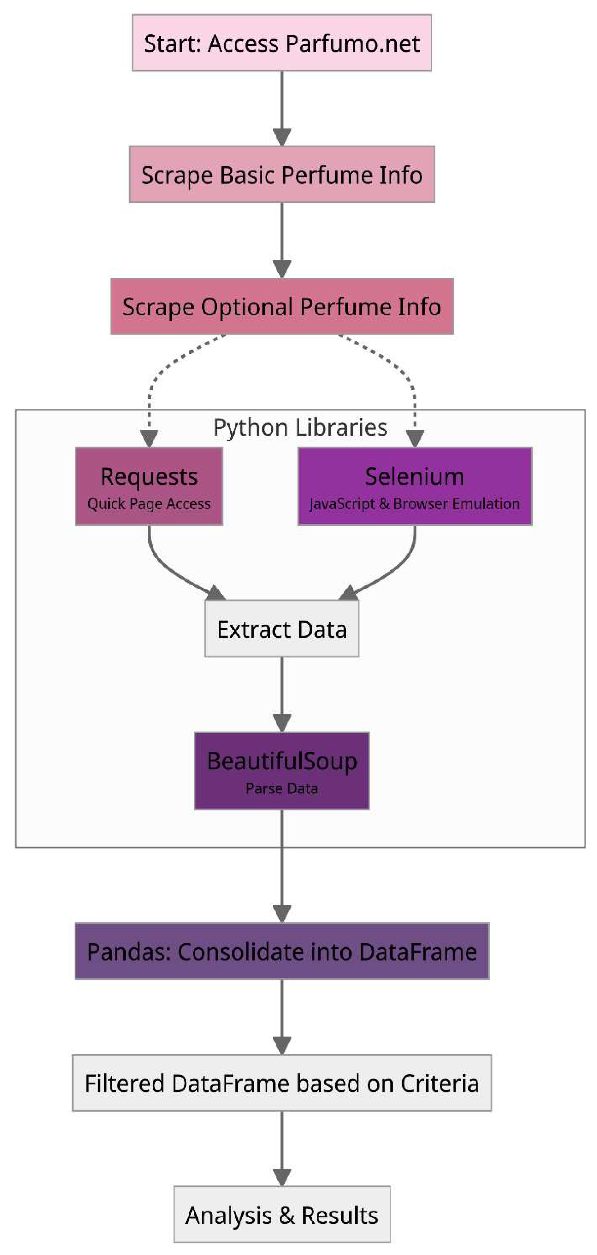
2.2. Database Clustering Using the k-Means Algorithm
2.3. Molecule Generation with GGNN
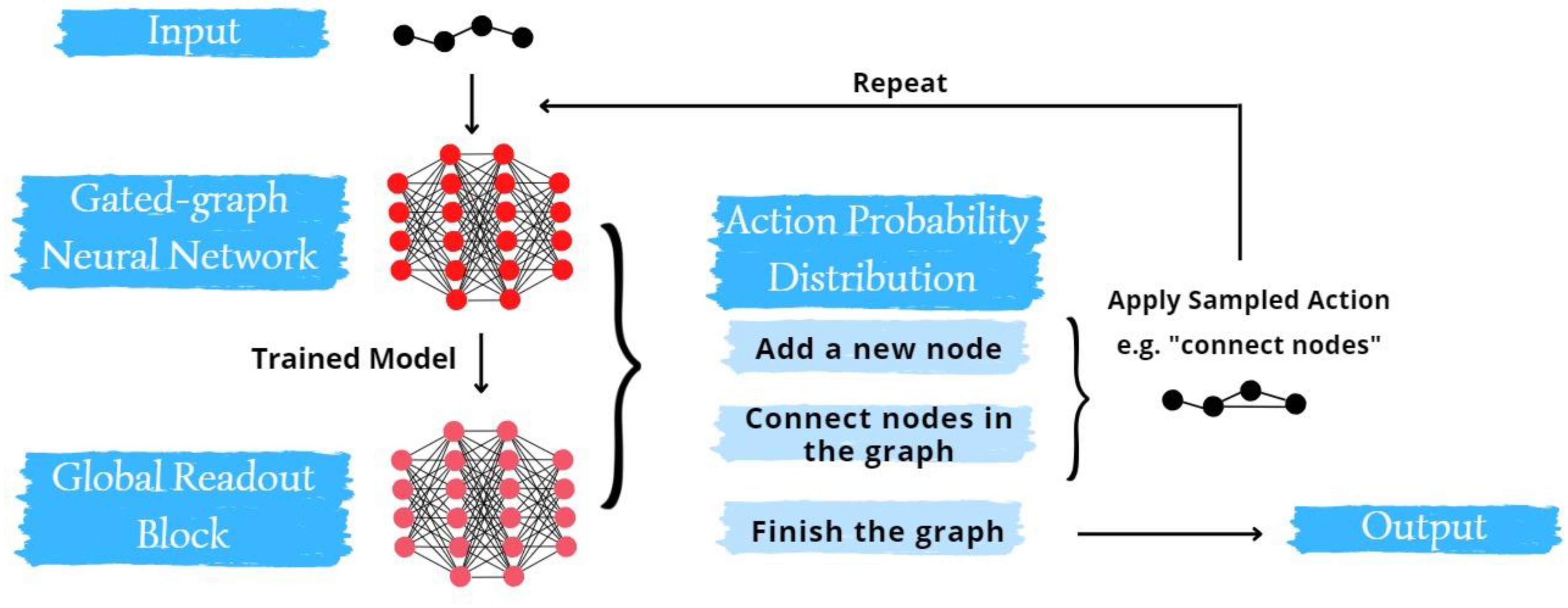
2.4. Molecule Generation for Desired Perfume Profiles and Assessment of Vapor Pressure
3. Results and discussion
3.1. Database and Statistics
3.2. Clusters
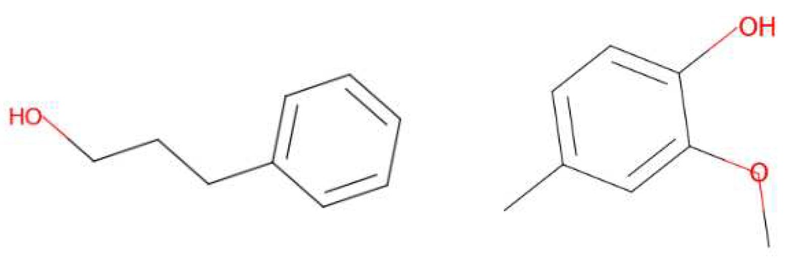
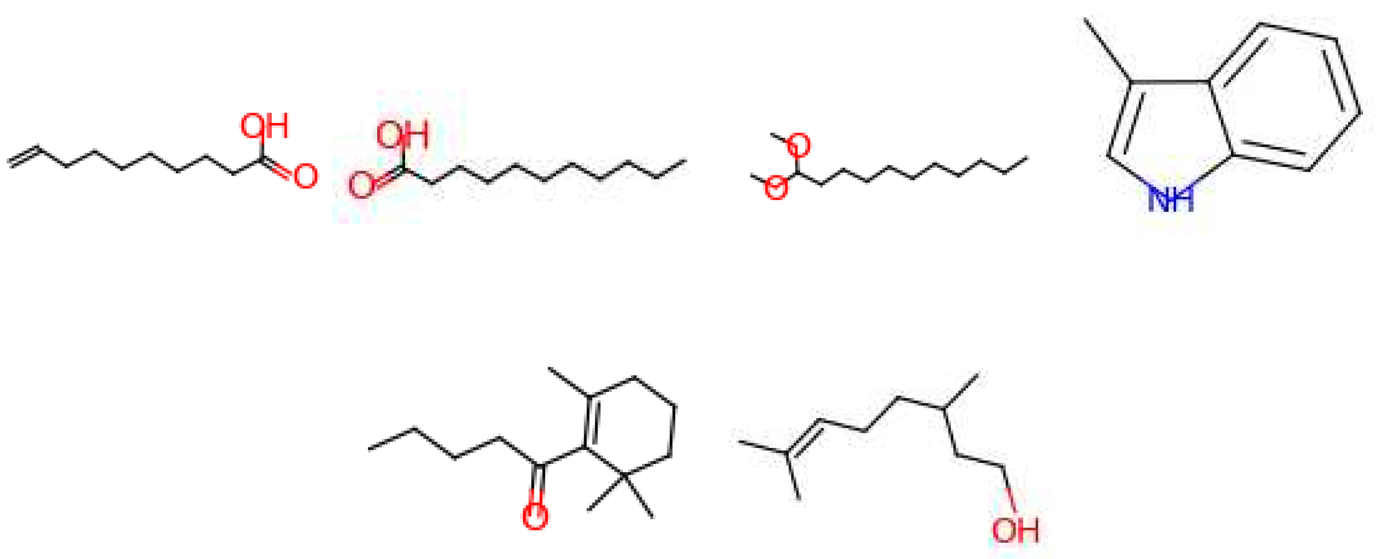
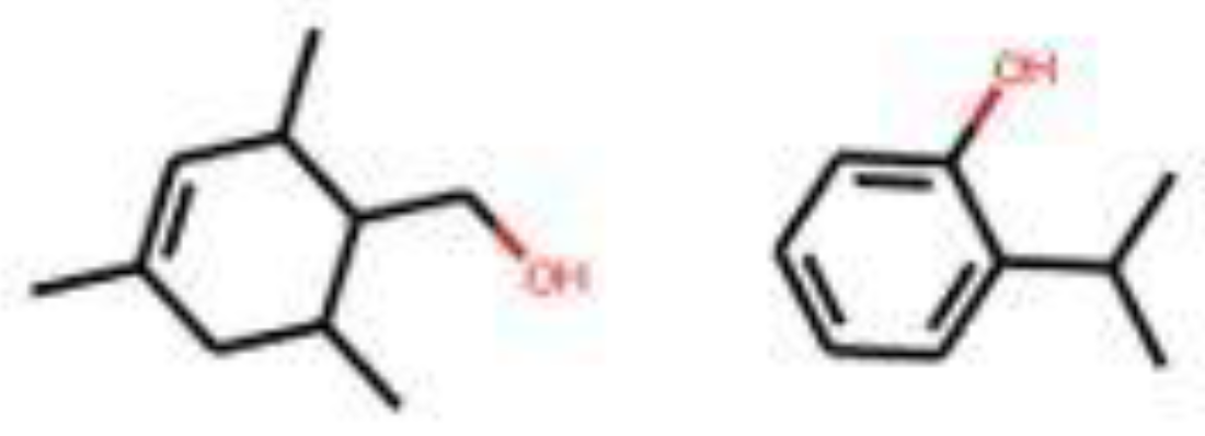
3.3. Generated Molecules
| Parameters | Value | Parameters | Value | Parameters | Value |
|---|---|---|---|---|---|
| A | 0.5 | GGNN width | 100 | MLP activation function | SOFTMAX |
| Batch size | 20 | Initial learning rate | 1x10⁻⁴ | MLP depth | 4 |
| Block size | 1000 | Learning rate decay factor | 0.99 | MLP droupout probability | 0 |
| Epochs | 500 | Learning rate decay interval | 10 | MLP hidden dimensions | 500 |
| Generation epoch | 1040 | Loss function | Kullback-Leibler divergence | Number of samples | 200 |
| GGNN activation function | SELU | Maximum relative learning rate | 1 | Optimizer | Adam |
| GGNN depth | 4 | Message passing layers | 3 | Sigma | 20 |
| GGNN dropout probability | 0 | Input size of GRU | 100 | Weight decay | 0 |
| GGNN hidden dimension | 250 | Minimum relative learning rate | 1x10⁻⁴ | Weight initialization | Uniform |
4. Conclusion
References
- Almeida, R. N., Costa, P., Pereira, J., Cassel, E., & Rodrigues, A. E. (2019). Evaporation and Permeation of Fragrance Applied to the Skin. Industrial & Engineering Chemistry Research, 58(22), 9644–9650. [CrossRef]
- Arús-Pous, J., Johansson, S. V., Prykhodko, O., Bjerrum, E. J., Tyrchan, C., Reymond, J.-L., Chen, H., & Engkvist, O. (2019). Randomized SMILES strings improve the quality of molecular generative models. Journal of Cheminformatics, 11(1), 71. [CrossRef]
- Bell, C. and C. (2023). Thermo: Chemical properties component of Chemical Engineering Design Library (ChEDL). https://github.com/CalebBell/thermo.
- Beyer, K., Goldstein, J., Ramakrishnan, R., & Shaft, U. (1999). When Is “Nearest Neighbor” Meaningful?.
- Bisong, E. (2019). Google Colaboratory. In Building Machine Learning and Deep Learning Models on Google Cloud Platform (pp. 59–64). Apress. [CrossRef]
- Bushdid, C., Magnasco, M. O., Vosshall, L. B., & Keller, A. (2014). Humans can discriminate more than 1 trillion olfactory stimuli. Science, 343(6177), 1370–1372. [CrossRef]
- Campolucci, P., Uncini, A., & Piazza, F. (1996). Causal back propagation through time for locally recurrent neural networks. 1996 IEEE International Symposium on Circuits and Systems. Circuits and Systems Connecting the World. ISCAS 96, 531–534. [CrossRef]
- Carles, J. (1961). A Method of Creation & Perfumery.
- Debnath, T., & Nakamoto, T. (2022). Predicting individual perceptual scent impression from imbalanced dataset using mass spectrum of odorant molecules. Scientific Reports, 12(1). [CrossRef]
- Fortune Business Insight. (2022, May). Flavors and Fragrances Market Size, Share & COVID-19 Impact Analysis.
- Gerkin, R. C. (2021). Parsing Sage and Rosemary in Time: The Machine Learning Race to Crack Olfactory Perception. In Chemical Senses (Vol. 46). Oxford University Press. [CrossRef]
- Kingma, D. P., & Ba, J. (2014). Adam: A Method for Stochastic Optimization.
- Kullback, S., & Leibler, R. A. (1951). On Information and Sufficiency. The Annals of Mathematical Statistics, 22(1), 79–86. http://www.jstor.org/stable/2236703.
- Leffingwell & Associates. (2018). Flavor & Fragrance Industry - Top 10. Flavor & Fragrance Industry - Top 10.
- Li, Y., Tarlow, D., Brockschmidt, M., & Zemel, R. (2015). Gated Graph Sequence Neural Networks.
- Mata, V. G., Gomes, P. B., & Rodrigues, A. E. (2005). Engineering perfumes. AIChE Journal, 51(10), 2834–2852. [CrossRef]
- Nozaki, Y., & Nakamoto, T. (2018). Predictive modeling for odor character of a chemical using machine learning combined with natural language processing. PLoS ONE, 2008, 13(6). https://www.parfumo.com/. [CrossRef]
- Parfumo.
- Queiroz, L. P., Rebello, C. M., Costa, E. A., Santana, V. V., Rodrigues, B. C. L., Rodrigues, A. E., Ribeiro, A. M., & Nogueira, I. B. R. (2023a). A Reinforcement Learning Framework to Discover Natural Flavor Molecules. Foods, 12(6), 1147. [CrossRef]
- Queiroz, L. P., Rebello, C. M., Costa, E. A., Santana, V. V., Rodrigues, B. C. L., Rodrigues, A. E., Ribeiro, A. M., & Nogueira, I. B. R. (2023b). Generating Flavor Molecules Using Scientific Machine Learning. ACS Omega, 8(12), 10875–10887. [CrossRef]
- Queiroz, L. P., Rebello, C. M., Costa, E. A., Santana, V. V., Rodrigues, B. C. L., Rodrigues, A. E., Ribeiro, A. M., & Nogueira, I. B. R. (2023c). Transfer Learning Approach to Develop Natural Molecules with Specific Flavor Requirements. Industrial & Engineering Chemistry Research, 62(23), 9062–9076. [CrossRef]
- RDKit: Open-source cheminformatics. (n.d.). https://www.rdkit.org.
- Richardson, L. (2007). Beautiful soup documentation. April.
- Rodrigues, A. E., Nogueira, I., & Faria, R. P. V. (2021). Perfume and Flavor Engineering: A Chemical Engineering Perspective. Molecules, 26(11), 3095. [CrossRef]
- Rousseeuw, P. J. (1987). Silhouettes: A graphical aid to the interpretation and validation of cluster analysis. Journal of Computational and Applied Mathematics, 20, 53–65. [CrossRef]
- Saini, K., & Ramanathan, V. (2022). A Review of Machine Learning Approaches to Predicting Molecular Odor in the Context of Multi-Label Classication. [CrossRef]
- Santana, V. V., Martins, M. A. F., Loureiro, J. M., Ribeiro, A. M., Rodrigues, A. E., & Nogueira, I. B. R. (2021). Optimal fragrances formulation using a deep learning neural network architecture: A novel systematic approach. Computers & Chemical Engineering, 150, 107344. [CrossRef]
- Sinaga, K. P., & Yang, M.-S. (2020). Unsupervised K-Means Clustering Algorithm. IEEE Access, 8, 80716–80727. [CrossRef]
- Teixeira, M. A., Rodríguez, O., Mata, V. G., & Rodrigues, A. E. (2009). The diffusion of perfume mixtures and the odor performance. Chemical Engineering Science, 64(11), 2570–2589. [CrossRef]
- The Good Scents Company. (2021). http://www.thegoodscentscompany.com/.
- The Pandas Development Team (2020). pandas-dev/pandas: Pandas. Zenodo. [CrossRef]
- Wakayama, H., Sakasai, M., Yoshikawa, K., & Inoue, M. (2019). Method for Predicting Odor Intensity of Perfumery Raw Materials Using Dose–Response Curve Database. Industrial & Engineering Chemistry Research, 58(32), 15036–15044. [CrossRef]
- Weininger, D., Weininger, A., & Weininger, J. L. (1989). SMILES. 2. Algorithm for generation of unique SMILES notation. Journal of Chemical Information and Computer Sciences, 29(2), 97–101. [CrossRef]
- Wen, T., & Zhang, Z. (2018). Deep Convolution Neural Network and Autoencoders-Based Unsupervised Feature Learning of EEG Signals. IEEE Access, 6, 25399–25410. [CrossRef]
- Xue, D., Gong, Y., Yang, Z., Chuai, G., Qu, S., Shen, A., Yu, J., & Liu, Q. (2019). Advances and challenges in deep generative models for de novo molecule generation. WIREs Computational Molecular Science, 9(3). [CrossRef]
- Zhou, Z., Kearnes, S., Li, L., Zare, R. N., & Riley, P. (2019). Optimization of Molecules via Deep Reinforcement Learning. Scientific Reports, 9(1), 10752. [CrossRef]


| Leather | Iris | Cedarwood | Tonka bean | Frankincense | Vetiver | Rose | Jasmine | Bergamot | Patchouli | Amber | Sandalwood | Vanilla | Musk | |
|---|---|---|---|---|---|---|---|---|---|---|---|---|---|---|
| Unisex | 354 | 297 | 375 | 342 | 535 | 497 | 479 | 480 | 656 | 769 | 715 | 741 | 823 | 947 |
| Male | 137 | 54 | 100 | 92 | 80 | 202 | 48 | 77 | 256 | 213 | 230 | 213 | 133 | 242 |
| Female | 48 | 202 | 92 | 151 | 83 | 121 | 451 | 558 | 266 | 292 | 366 | 393 | 582 | 605 |
| Leather | Iris | Cedarwood | Tonka bean | Frankincense | Vetiver | Rose | Jasmine | Bergamot | Patchouli | Amber | Sandalwood | Vanilla | Musk | |
|---|---|---|---|---|---|---|---|---|---|---|---|---|---|---|
| Unisex | 10978 | 13436 | 16039 | 14513 | 19407 | 18097 | 15865 | 14268 | 21439 | 23906 | 28377 | 24897 | 30168 | 34312 |
| Male | 4935 | 5860 | 5517 | 3969 | 4360 | 10468 | 1577 | 1823 | 13677 | 10051 | 10051 | 5219 | 7445 | 7816 |
| Female | 2485 | 6786 | 3514 | 7105 | 3338 | 5913 | 13263 | 15201 | 11273 | 13691 | 13691 | 10636 | 17570 | 18320 |
| Leather | Iris | Cedarwood | Tonka bean | Frankincense | Vetiver | Rose | Jasmine | Bergamot | Patchouli | Amber | Sandalwood | Vanilla | Musk | |
|---|---|---|---|---|---|---|---|---|---|---|---|---|---|---|
| Unisex | 7,75 | 7,65 | 7,84 | 7,83 | 7,80 | 7,82 | 7,62 | 7,61 | 7,72 | 7,81 | 7,78 | 7,78 | 7,81 | 7,69 |
| Male | 7,52 | 8,15 | 7,65 | 7,65 | 7,82 | 7,69 | 7,70 | 7,66 | 7,55 | 7,89 | 7,53 | 7,53 | 7,79 | 7,64 |
| Female | 7,95 | 7,68 | 7,77 | 7,77 | 7,55 | 7,80 | 7,60 | 7,47 | 7,57 | 7,53 | 7,53 | 7,53 | 7,56 | 7,51 |
Disclaimer/Publisher’s Note: The statements, opinions and data contained in all publications are solely those of the individual author(s) and contributor(s) and not of MDPI and/or the editor(s). MDPI and/or the editor(s) disclaim responsibility for any injury to people or property resulting from any ideas, methods, instructions or products referred to in the content. |
© 2023 by the authors. Licensee MDPI, Basel, Switzerland. This article is an open access article distributed under the terms and conditions of the Creative Commons Attribution (CC BY) license (http://creativecommons.org/licenses/by/4.0/).


