1. Introduction
The significance of recommender systems has surged in the digital era, driven by the increasing consumer demand for assistance navigating an abundance of choices. These systems employ machine learning algorithms to identify evolving patterns in user behavior, subsequently leveraging this insight to present fresh recommendations to users [
1].
The Internet’s widespread use allows people to interact with social media, an essential part of our daily lives in the significant data world [
2]. In this way, users can share opinions, ideas, and comments about news, places, social events, and multimedia has become typical. Specifically, the movie domain represents a topic of interest due to its commercial value. That interest led to the creation of social media platforms, websites, and blogs where users and critics can share their opinions about any movie created.
Gaining insights into how audiences perceive television programs and movies is a crucial aspect of the entertainment industry. For instance, movie production companies and investors often seek audience feedback for the films they support. Evaluations from viewers can be instrumental in assessing various aspects, including the overall quality of a movie, the effectiveness of specific scenes, the impact of prevailing public opinion on the film’s success or failure, and recommendations for improving the movie. Additionally, this feedback can influence decisions related to future productions, such as casting choices for specific genres or selecting scenes to include in trailers to attract audiences. Ultimately, these considerations can lead to increased revenue for movie production companies.
Movie reviews are a valuable tool for users to assess and determine whether a specific film aligns with their preferences. Recently, a wealth of movie-related data exists, such as the extensive Internet Movie Database (IMDb), which houses thousands of movie reviews. Nonetheless, manually scrutinizing each of these reviews can be a laborious and time-consuming task. Hence, integrating machine learning models offers a potential solution for efficiently automating and analyzing these reviews.
Thus, IMDb is one of the top popular online sites and databases for movies and TV shows. This platform provides a collection of datasets with important information about films and shows, such as crew, cast, rating, age categories, types, genres, reviews, or summaries [
3]. Anyone can access this information and analyze the aspects they are interested in the most, such as estimated characteristics of blockbusters or flops.
Furthermore, part of this analysis relies on natural language processing (NLP) tools to gather information from user reviews and ratings. The most popular dataset is the IMDb for sentiment analysis, consisting of 50,000 reviews labeled as positive or negative, created by [
4], employing natural language techniques such as semantic similarities among words and a probabilistic model for word representations.
Other popular datasets are “The movie dataset” by Rounak Banik [
5], containing principally rating and metadata but no text data information, and “IMDb Dataset of 50K Movie Reviews” by Lakshmi Pathi [
6] being composed of movie metadata and reviews from 50,000 movies.
Most of these datasets are not curated; the data are extracted, but the opinions may be diverse and unable to reflect the genre of the movie reviewed. It generates a problem when a class is misrepresented due to a lack of consistency or unbalanced data per class.
These are common issues with short texts serving as opinions, and mostly with data scrapped from the web, topics or classes might need to be labeled correctly, resulting in an imbalanced dataset [
7].
According to Unal et al. (2023) [
8] multilabel classification is attributing multiple labels or tags to a given input instance. In the specific domain of movie films, this task involves recognizing and allocating appropriate genre labels to posters based on their visual attributes. Film genres, such as action, romance, comedy, horror, sci-fi, and numerous others, encompass the diverse spectrum of cinematic offerings, each characterized by distinct visual elements and themes. The ability to automatically categorize movie films into multiple genres not only streamlines the process of cataloging and organizing but also unlocks opportunities for tailored recommendations, genre-focused marketing approaches, and enriched user interactions within cinema.
The objective of the proposed work is to analyze the effect of removing stop-words by different methods on text classification to obtain the true genre from the user reviews using K-means clustering.
The rest of the paper is structured as follows:
Section 2 comprises the literature review on text classification approaches in movie reviews by genre,
Section 3 describes the methodology and the proposed methods concerning clustering and analysis of movie reviews,
Section 4 presents the experimental results, and the last section discusses the essential findings and conclusion of our research.
2. Related Work
The clustering analysis of movie reviews based on their genre is not a trivial task. There are research studies that apply natural language processing, combining machine learning techniques to classify movie datasets.
Thus, Battu et al. (2018) [
9] created a multi-language dataset, extracting summaries from nearly 15 000 movies. They grouped 27 genres into nine genre classes according to which genre belongs to each primary class. For instance, genres like Action, Adventure, Sci-fi, Sport, or War were labeled “Action”. Unfortunately, they did not report the performance for each class to see if grouping genres helped to reduce the misclassification in classes with little data.
Ka-Wing Ho (2011) [
10] tested different methods to classify movie genres based on the synopsis. The dataset comprised 16,000 unique movies labeled with the ten popular genres. The evaluation with machine learning techniques showed that genres with little data are prone to be misclassified.
Quan Hoang (2018) [
11] explored various machine and deep learning techniques, using a corpus with up to 250,000 summaries from IMDb films, contemplating 20 different genres since each review is tagged the same as the movie’s original genre is hard to identify genres with few inputs like “War” correctly. It is a common problem with short texts serving as opinions. The topic might be mislabeled, and the dataset imbalanced.
Recently, a more significant movie review dataset was released, containing nearly 1 million unique reviews from 1,150 different IMDb movies, including metadata, and focused on 17 genres. The high amount of data improved the overall machine and deep learning classification score. However, there is no information about performance by genre. Similar to other movie review datasets, genres like “War” or “Western” have fewer entries compared to most popular genres such as “Action” or “Drama” [
12].
In [
13], the Gold Standard corpus was created and reviewed by experts to ensure proper data annotation in general text classification tasks. Some corpora for text classification are widely used to test new machine learning classification algorithms like the AG’s news corpus [
14] or the DBPedia [
15]. However, a gold standard for movie reviews and genre classification is still missing.
Thus, one solution to avoid mislabeling or poor annotation in large datasets is to rely on text clustering. Cluster analysis is the unsupervised process of grouping data instances into relatively similar categories without understanding the group’s structure or class labels [
16].
Several clustering algorithms help to classify similar text documents together. The most crucial clustering algorithms are K-means, K-medoids, Fuzzy, Hierarchical, and density-based. K-means and K-medoids are the most popular hard clustering algorithms [
17]. Both have proved to be suitable and adequate for natural language processing tasks.
Rose et al. (2020) [
18] created a framework to pre-process and cluster aviation safety reports promising to support detection trends and anomalies from an extensive database. They employed a combination of TF-IDF and K-Means clustering. Their pre-processing included basic cleaning, NTLK stop-words removal, and stemming. They encountered issues reflecting the success of clustering text-based data with the Silhouette score and Calinski-Harabasz method.
Researchers spend vast amounts of time manually sorting out scientific databases for tasks such as systematic literature reviews. Weißer et al. (2020) [
19] proposed applying NLP standard techniques to article metadata. The process employed TF-IDF and K-means clustering algorithms to separate large text datasets into several groups based on their topics. Adinugroho et al. (2020) [
20] built a similar protocol, including term-clustering weighting and modifying the K-Means algorithm called Pillar K-Means, generating good results.
Although TF-IDF is one of the most employed vectorization techniques, some authors have proved different approaches. Kumari and Shashi (2019) [
21] applied various vectorization methods such as Word2vec and Doc2Vec, along with K-Means clustering a multidimensional scaling representation. The final results favored the TF-IDF vectorization, concluding that this technique granted the highest purity cluster formation.
Soni and Mathai (2015) [
22] employed unsupervised learning through K-means clustering to cluster tweets. After performing supervised learning methods, they extracted features using a simple Bag of Words technique. In this way, the ‘Cluster-then-predict Model’ hybrid method has improved the accuracy of predicting Twitter sentiment.
Zhao (2012) [
23] showed various case studies using tweets in the timeline of data mining with both K-means and K-medoids algorithms. In general, K-means performed better in separating text data by topics, and the clusters’ features were defined better, allowing us to quickly find what the group was about.
Other clustering algorithms, such as hierarchical or agglomerative, were tested for similar tasks by Kaur (2015) [
24] and Miyamoto et al. (2012) [
25]. However, these approaches counted occurrences of specific nouns or word sequences. The downside is the long runtime limiting the use of arguably small datasets.
Kadhim et al. (2014) [
26] proposed a combination of TF-IDF weighing and dimension reduction before clustering. In this way, his proposed method helped to reduce the dimensionality, and the accuracy was almost the same.
Fodeh et al. (2021) [
27] proposed a multi-class classification approach to categorize Twitter chatter based on the motive of opioid misuse. They collected nearly 7,000 tweets and manually annotated them into three classes. The vector representations were generated using Word2Vec and clustered with K-means algorithms. This work with distinct clustering of class-specific keywords may enable targeted data collection, significantly aiding the under-representation of minority classes.
Thus, we propose an unsupervised classification for movie reviews implementing different pre-processing protocols, TF-IDF vectorization, Word2Vec embeddings, K-means clustering, and dimensionality reduction with Principal Component Analysis (PCA) to annotate a movie review dataset extracted from IMDb. Ideally, clusters reflect highly similar reviews; their principal features will allow us to identify the genre. Machine learning techniques will test the resulting annotated datasets to evaluate their accuracy, recall, precision, and F-1 score.
3. Materials and Methods
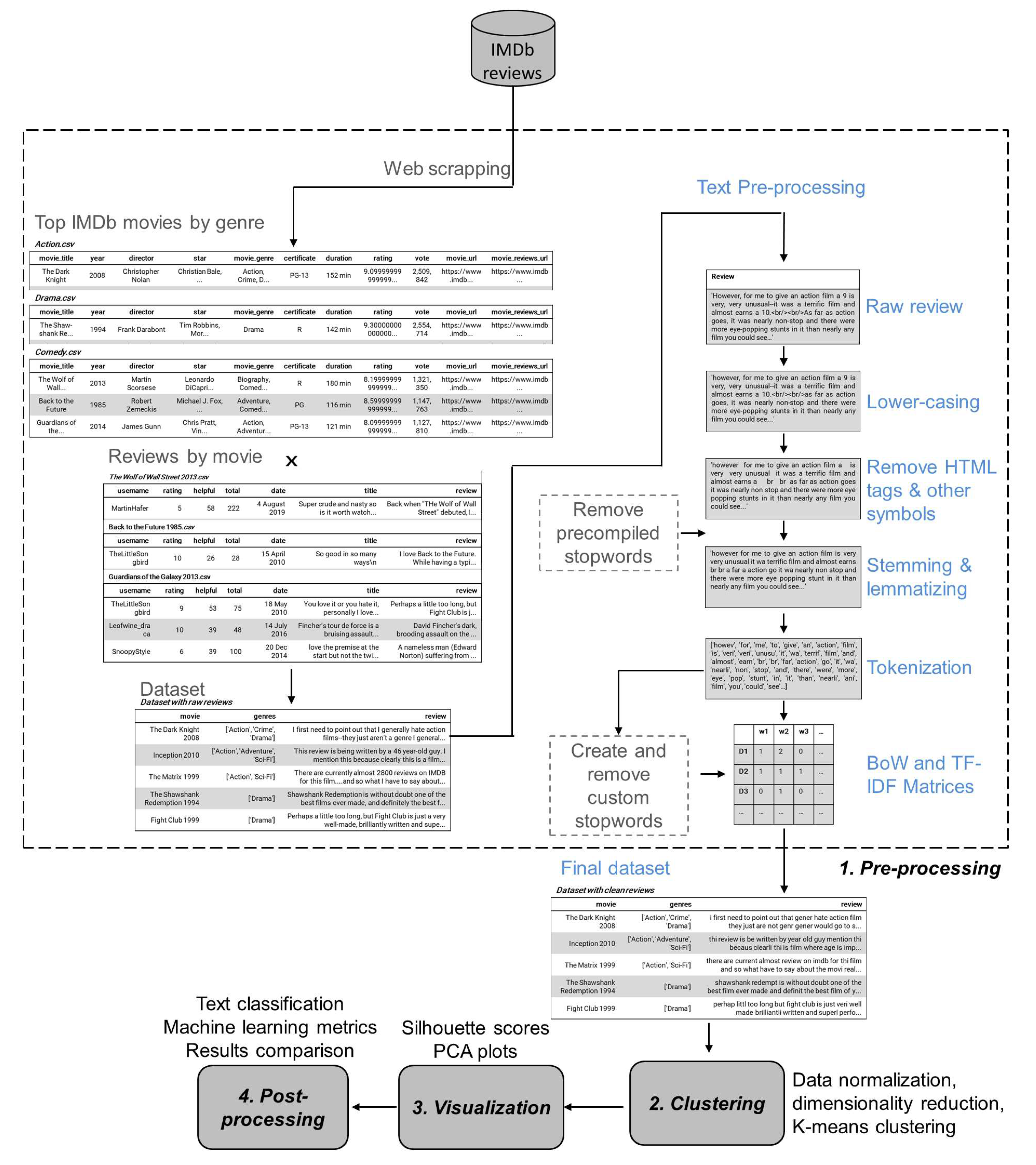
This work aims to create a model for genre prediction using movie reviews from Internet Movie Database IMDb.
Figure 1 presents the proposed general framework and the stages involved in the analysis.
3.1. Data Collection
To create the dataset, we used Python scraping libraries to extract movie details from the list of top IMDb movies belonging to 18 movie genres – Action, Adventure, Animation, Biography, Comedy, Crime, Drama, Fantasy, History, Horror, Music, Mystery, Romance, Sci-Fi, Sport, Thriller, War and Western. We retrieved up to 3.5 million raw reviews from 3,688 unique movies using Python web scrapping libraries; movies with less than 20 reviews were ignored. Additionally, we removed reviews with less than 50 words or more than 500.
3.2. Text Preprocessing
Raw review files were cleaned with preprocessing tools for noise reduction. The cleaning included removing HTML tags, special characters, different short and long words, lemmatization and stem, and removing stop-words as depicted in
Figure 1. In addition, stop-words were retrieved from NLTK, ISO project, Genrec, or custom extracted by word frequency across the documents.
3.2.1. Removal Methods for Stop-Words
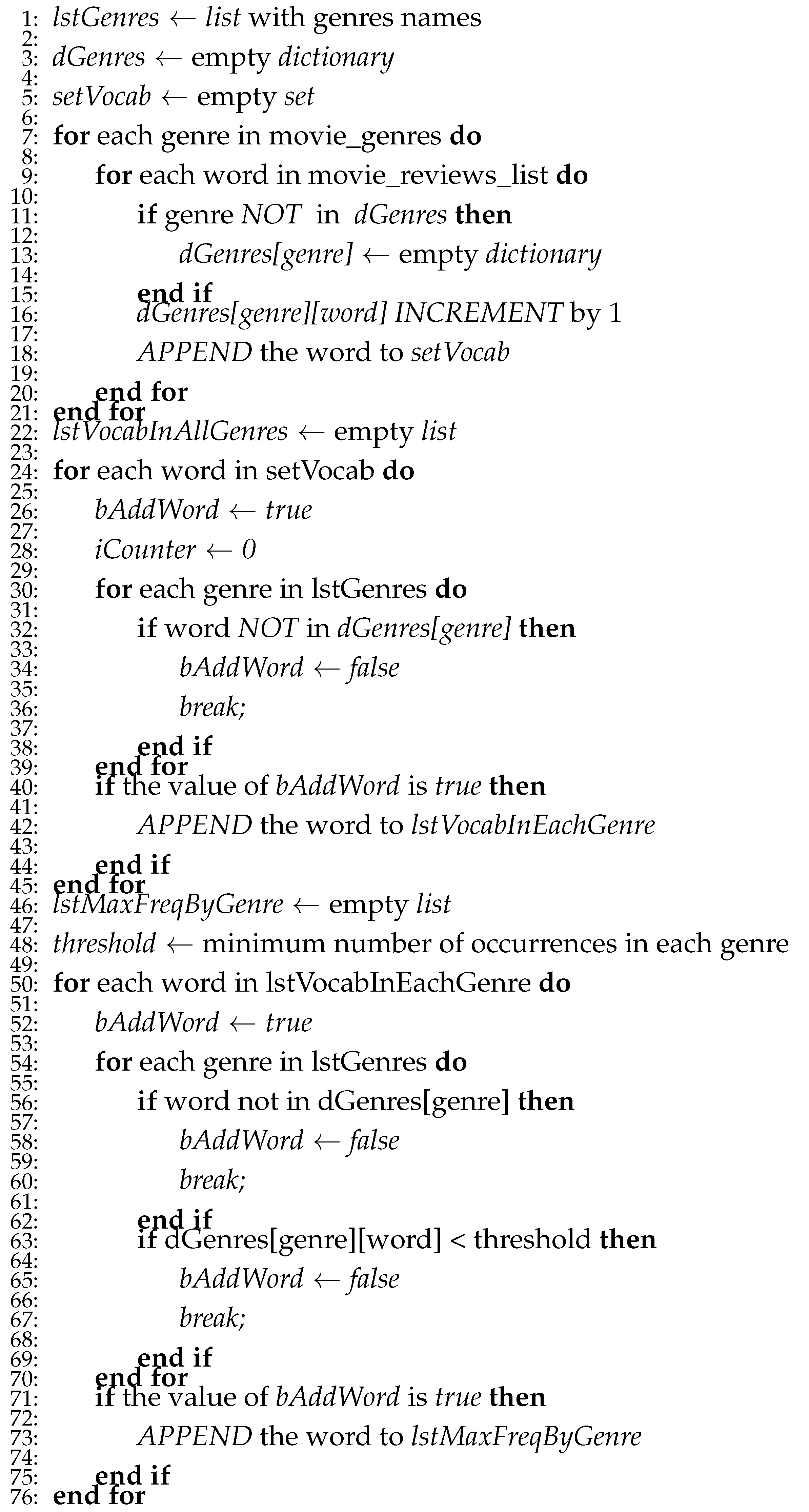
Table 1 summarizes the methods employed to remove stop-words. Our proposed method "Threshold" described in Algorithm 1 is divided into three main steps:
- (a)
Iterate the list of genres against the movie reviews to create a vocabulary without repeated words and the counter of each term for each genre.
- (b)
Iterate the vocabulary without repeated words against the list of genres, and if the word is in all the genres, then the word is added.
- (c)
Finally, a threshold is set (minimum times a word must appear in each genre to be added). Iterate the vocabulary list in each genre against the list of genres. If the word is in all the genres and the word occurrences are equal or greater than the threshold, then the word is added.
With these steps, a list of stop-words is generated to be removed from the dataset subsequently.
|
Algorithm 1 Threshold method. |
 |
3.2.2. TF-IDF method
Term frequency–inverse document frequency (TF-IDF) is a numerical statistic that reflects a word’s importance to a document in a collection or corpus [
31]. TF-IDF is the product of two statisctics,
term frecuency and
inverse document frecuency. Thus, term frequency,
is the relative frequency of the term
t within document
d.
Where is the raw count of a term in a document, i.e., the number of times that term t occurs in document d.
On the other hand, inverse document frequency measures how much information the word gives, whether it is a common word in all documents or a rare one. It is defined as the logarithmically scaled inverse fraction of the documents that contain the word:
Where:
Finally, combining the two formulas above, we have the term frequency-inverse document frequency:
3.2.3. Word2Vec Method
One problem with text classification is that the bag-of-word (BoW) feature and the conditional independence assumption need to be revised to capture the meaning of sentences in the text. Therefore, we employed rich, contextual representations for words learned by the word2vec framework [
32]. Each review is turned into a vector representation by taking the average of the embedding vectors of all words in each text. The assumption is that the average vector can be an excellent semantic summarization of the review.
3.3. Clustering Approaches
In early 1939, the first clustering algorithms were developed due to the need to classify data. Social and biological sciences began searching for an automatized and organized manner to divide information into more approachable groups or clusters with similar characteristics. The first two mentioned algorithms were based on partitions and hierarchies [
33].
Nowadays, clustering algorithms have emerged as a powerful tool to accurately analyze the great amount of data generated by modern applications in a large variety of fields, such as: biology [
34], medicine [
35], business and marketing [
36], world wide web [
37], social science [
38], and computer science [
39].
The natural language processing involves grouping similar documents or sentences based on their content. Therefore, organizing large amounts of unlabeled or mislabeled text data into meaningful clusters is possible. As summarized by [
40], clustering algorithms can be divided into partitioning-based, hierarchical-based, density-based, grid-based, and model-based (see
Table 2).
Many authors have tested different clustering algorithms to analyze text data. For example, [
18] concluded that between hierarchical clustering, DBSCAN clustering, and K-means, the latest provided the most precise results with the most distinct and relevant clusters and was selected as their main algorithm. The K-means algorithm has been widely used in the field of NLP mainly to analyze short texts like tweets [
27,
41], web-short snippets [
42], questions [
42], news [
21,
43], and biomedical texts [
42]. Thus, K-means clustering is an adequate and widely used tool for analyzing text data.
3.3.1. K-Means Clustering
K-means clustering lies in the partitioning clustering method most frequently used in data mining; the algorithm segregates N number of documents into K number of clusters, while the value of K is specified by users or determined by methods such as elbows. Thus, the true K will be used to partition our N documents in K different classes in which documents of the same cluster must be similar and dissimilar from the other clusters or classes using some similarity formulas like Euclidean or Cosine similarity.
This clustering algorithm aims to decrease the summation of square distance among data points and their respective cluster centers or
centroids. The computing steps required for the K-means clustering method were defined by [
44]. Thus, selecting the initial
K cluster centers as:
Now, to distribute the data
X in
K clusters at
iteration, we used the following relation:
For all
;
; where
represents the set of data points whose cluster centers is
. Calculate the new center
as the summation of the squared distances to the new cluster center from all points in
minimized. The part that works to reduce the distance is simply the mean of
. Thus, the new cluster center is computed as follows:
While the stands for the number of samples in , if for , then the algorithm become halt due to converged action, otherwise repeat second step (5).
In this process, it is clear that the final clustering results are always affected by the initial seed and actual value of K. Still, initial seeds and the true value of K present in the dataset required previous knowledge, which is mostly impractical.
3.3.2. Mini Batch K-means
Mini Batch K-Means algorithm was used as a variant of the standard K-Means clustering algorithm [
45]. Mini-batches are subsets of the input data, randomly sampled in each training iteration. These mini-batches drastically reduce the computation required to converge to a local solution. In contrast to other algorithms that reduce the convergence time of k-means, mini-batch k-means produce results that are generally only slightly worse than the standard algorithm. Therefore, it allows us to calculate common metrics to estimate the ideal number of clusters like inertia (Elbow) [
46], Silhouette [
47], or Calinski-Harabasz score [
48].
We decided to use the Silhouette score as it gives good results in practice [
49]. Silhouette score is a reliable metric to predict the adequate number of clusters. Thus, we decided to use it to evaluate our datasets. The Silhouette coefficient is computed as follows:
Where a corresponds to each sample’s mean intra-cluster distance (a) and the mean nearest-cluster distance (b), the best value is 1, and the worst value is -1. Values near 0 indicate overlapping clusters.
The MiniBatch K-means algorithm was employed for all datasets to predict the optimal cluster number. Once they were obtained, the standard K-mean algorithm was run with each dataset’s predicted number of clusters.
3.4. Visualization Stage
All plots were generated with matplotlib.pyplot from Python. Principal Component Analysis (PCA) was employed to represent dimensionally reduced data. Statistical analysis was performed and annotated with Python library statannotations. For all column analysis, t-test for independent samples was used to compare to groups.
3.5. Post-Processing Stage
In this stage, we made the text classification post-processing, considering machine learning techniques to optimize the classification task.
Thus, we employed two of the most efficient classifiers from Sklearn to use as base models. Data was divided into train and test datasets with a relation 8:2. The following subsections describe the methods that provided better results in the case study.
3.5.1. Logistic Regression Approach
It is a statistical model that uses a logistic function to model a binary dependent variable (see Equation (
8)).
If the -z exponent tends to be minus infinity, we have a minimum value close to 0. If the -z exponent tends to positive infinity, the value tends to be 1. Values between 0 and 1 give us the probability of the function [
50]. Given the asymptotic nature of the logistic function, it can lead to a loss close to 0 when the dimensions are enormous. Therefore, most logistic models use regularization strategies like L2 or reduce the number of cycles/epochs in training.
3.5.2. Support Vector Machine Approach
The support vector machines (SVM) are supervised algorithms employed for classification and regression tasks. Support vector machines classify the data by finding a hyperplane that maximizes the margin between the classes in training the data. In a two-dimensional example with two classes, we can think of the hyperplane as the line that separates the two classes [
51].
During the model performance, the separating hyperplane is one of the probable planes separating the two classes. SVM finds an optimal hyperplane by distinguishing the two classes, using Equation (
9), proposed by [
52].
Subject to the following constraints:
Where w is a coefficient vector, b is the offset of the hyperplane from the beginning, is the positive slack variable, and signifies the penalty parameters of the errors.
3.5.3. Evaluation Metrics
Machine learning classifiers summarize the performance of each text classifier on the test dataset and evaluate the results into the following metrics: micro-average precision, micro-average recall, and micro-average F-score. The definition of these metrics is as stated in [
12].
Where represents the true positive values, indicates the false negative values and describes the false positives after the processing.
Moreover, to compute the prediction score of each text classifier method, we employed Equation (
15).
Where is the number of clusters defined as a genre and C is the total number of clusters.
On the other hand, concerning the statistical analysis, data are the means plus standard deviation, calculated and annotated with statannotations package. A is marked as significant.
4. Experimental Results
With Python web-scrapping libraries, we retrieved up to 4 million reviews from IMDd, tagged with one to three genres each. The majority of reviews dropped between ’Drama’ and ’Comedy’. We sought to balance this dataset to have a similar number of reviews by genre (see
Table 3).
In addition, we produced 25 datasets cleaned with different stop-words lists and vectorized either with TF-IDF or embedded with Word2Vec before clustering (see
Table 4). For each dataset, the ideal quantity of clusters was estimated and assessed by Mini Batch K-Means and Silhouette scores. Each cluster’s top features were selected to evaluate whether they belonged to a specific movie genre.
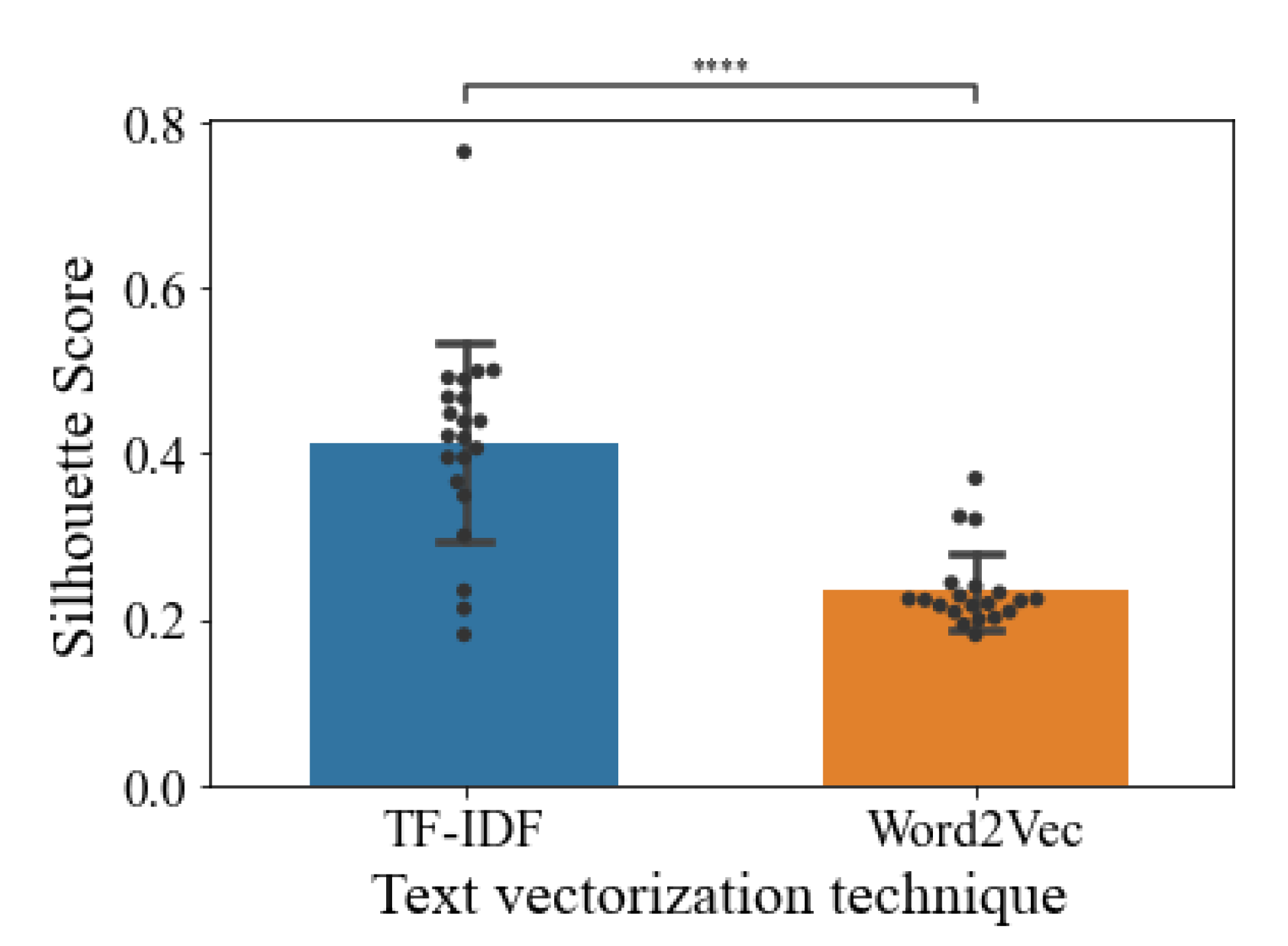
First, we compared the effect of tokenization on the clustering performance (see
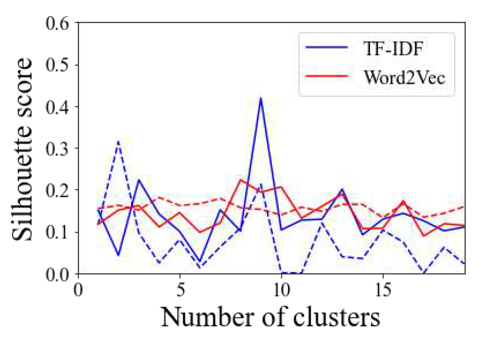
Figure 2). Generally, tokenization with TF-IDF (mean= 0.42 ± 0.11) resulted in higher Silhouette scores than Word2Vec (mean= 0.24 ± 0.06). Here, we show an example of the scores generated by the process (see
Figure 3).
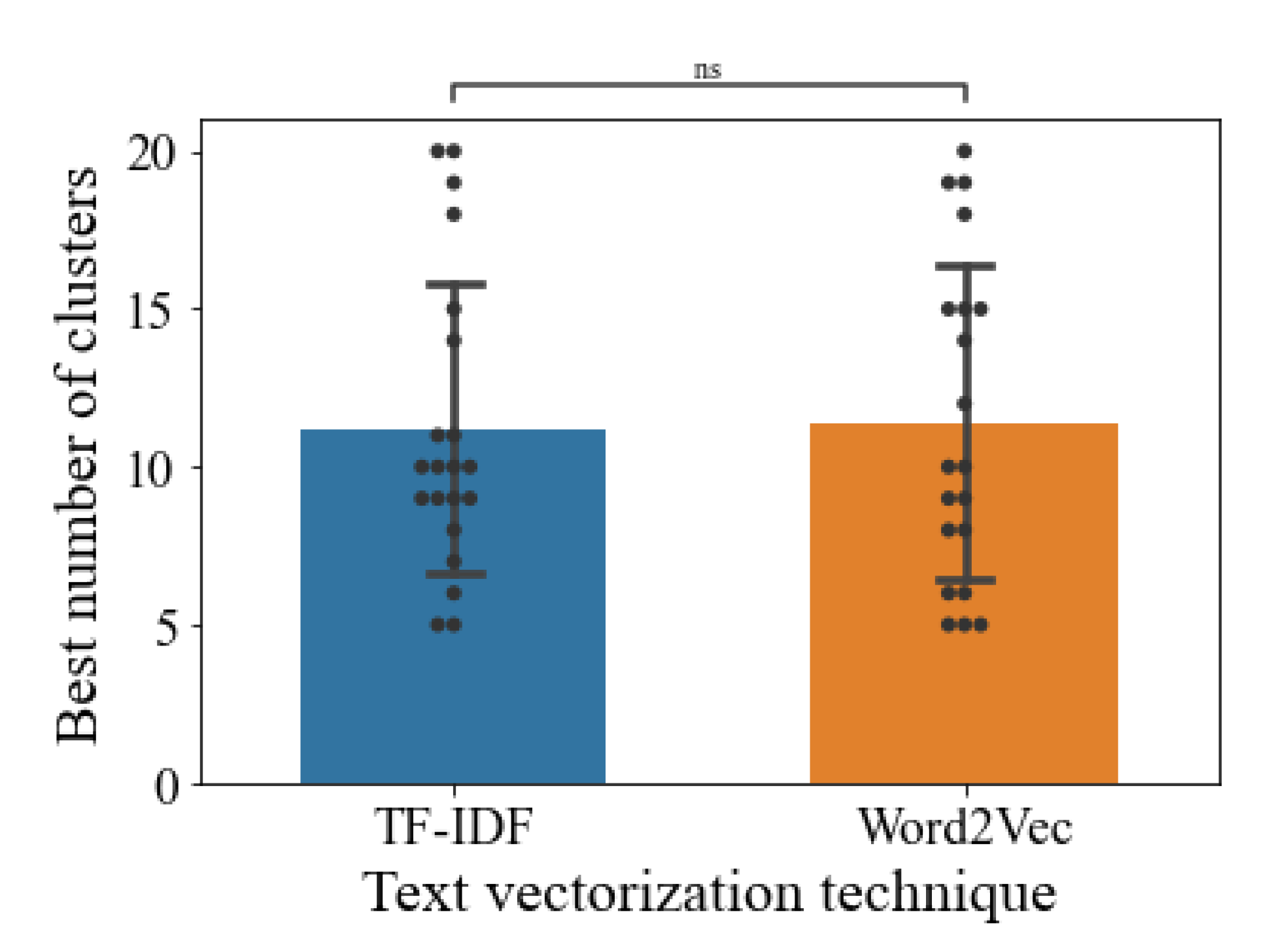
On the other hand, we analyzed the effect of the tokenization on the estimation of the number of clusters with TF-IDF (mean= 12.42 ± 5.16) or Word2Vec (mean= 11.71 ± 4.84) (see
Figure 4). Moreover,
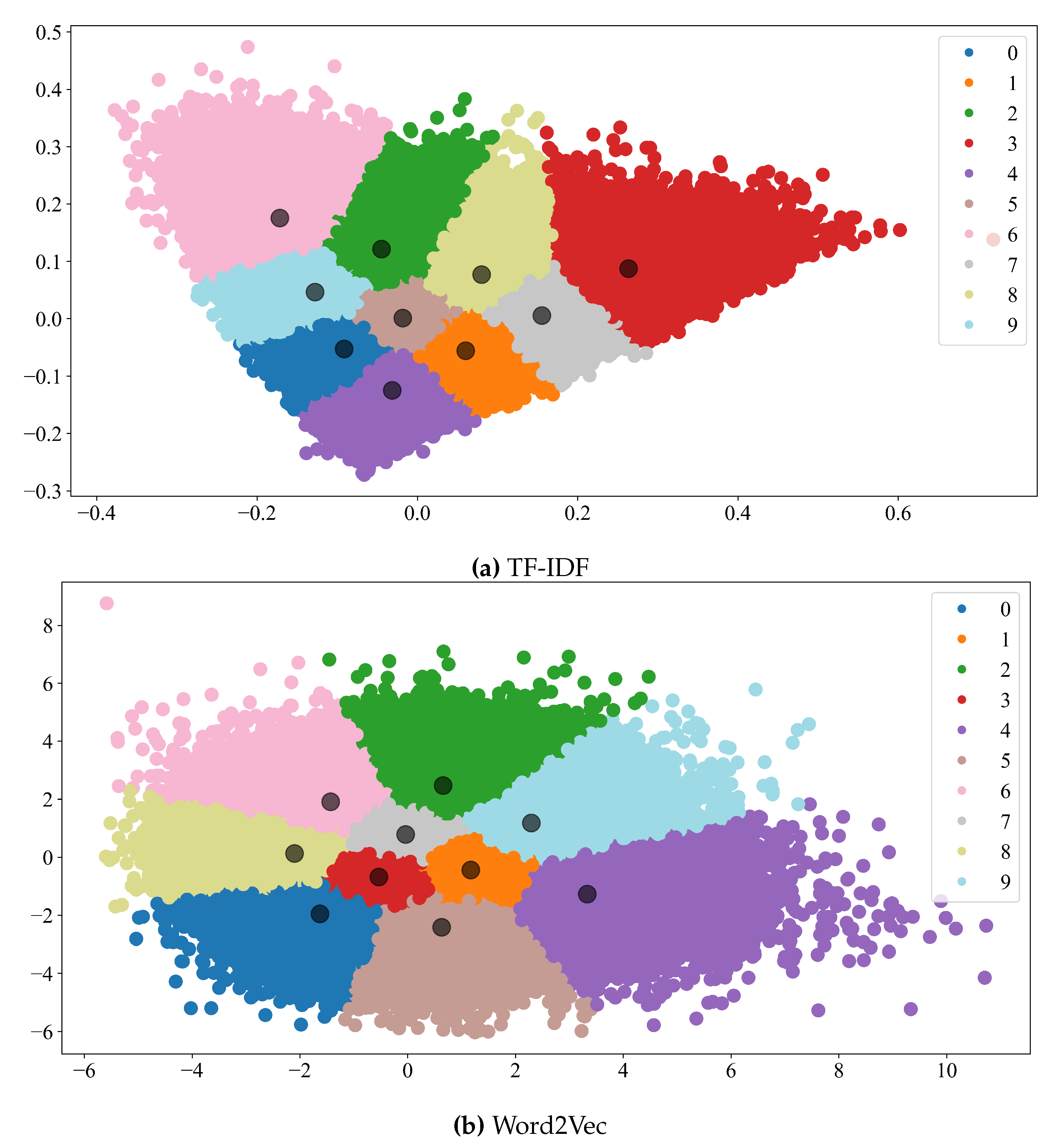
Figure 5 depicts an example of the clusters formed with TF-IDF or Word2Vec. Although clusters might look fine, we did not find a significant difference regarding the top features in each cluster comparing TF-IDF (see
Table 5) against Word2Vec (
Table 6). TF-IDF text vectorization granted features easily relatable to movie genres, whereas Word2Vec repeated similar words all over the different clusters.
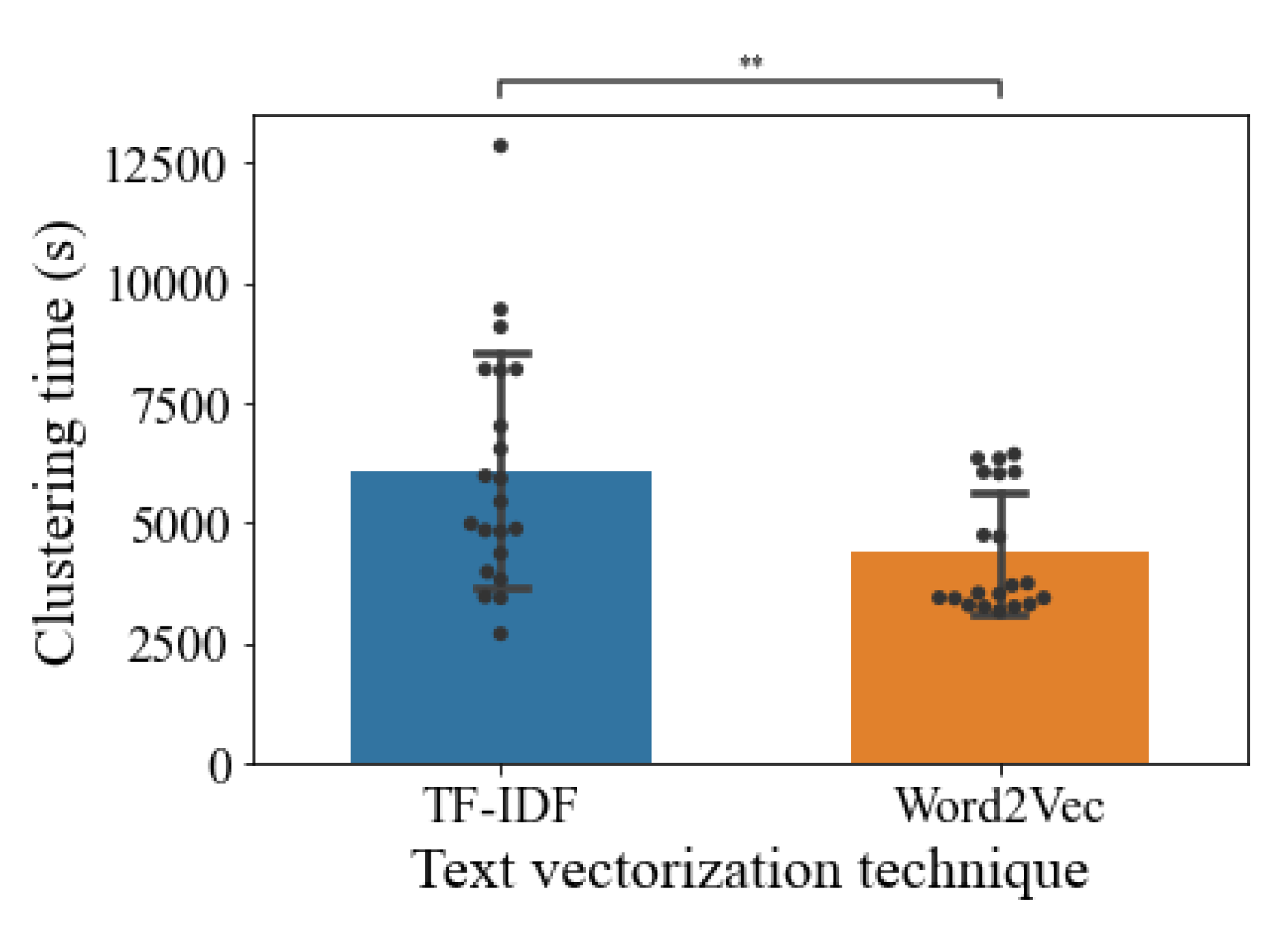
Thus, we resembled the effect of tokenization on the clustering time (see
Figure 6). Globally, the effect of the text vectorization method showed that TF-IDF (mean= 5,784.33s ± 2,524.19s) took more time than Word2Vec (mean= 4,268.04s ± 1,213.17s) in the clustering time took by Mini Batch K-Means.
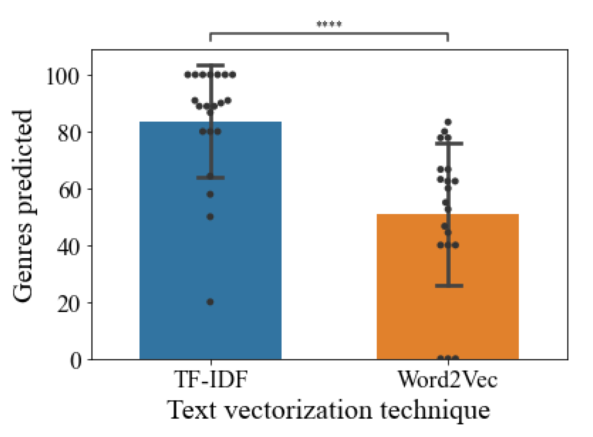
Furthermore, we were capable of predicting if a cluster could identify a specific movie genre by the top features in each cluster, similar to the previous results, using TF-IDF (mean= 81.34 ± 20.48) before running the K-means clustering resulted in more identifiable genres than when Word2Vec was used (mean= 53.51 ± 24.1) (see
Figure 7).
Concerning the balanced datasets, they improved results when training a machine learning model [
53]. We tested our different datasets using a Logistic regression model and a linear Support Vector Machine.
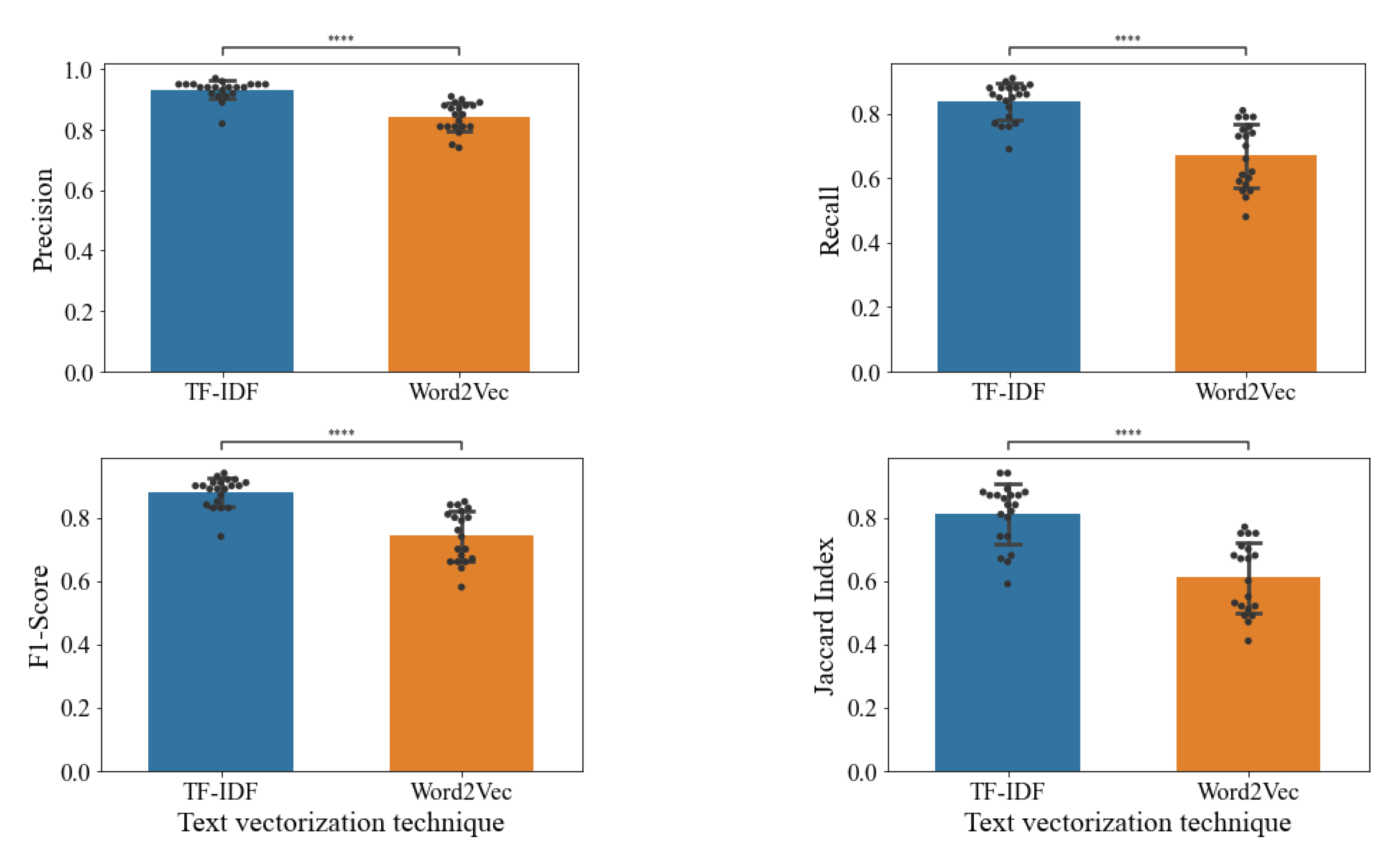
Firstly, we noticed that similarly to clustering, metrics such as Precision, Recall, F1-score, and Jaccard Index were higher while using TF-IDF prior clustering algorithms with the Logistic regression classifier (see
Figure 8). Due to our data distribution, we preferred the F1-score instead of Accuracy. The F1-score is especially suitable for our data because it is composed of uneven class distribution. Accuracy works better if the classes are well-balanced; that is not true for our datasets. Most popular genres contain most of the data, like ’Comedy’ or ’Drama’, whereas others, like ’Sci-Fi’ or ’Fantasy’, have fewer reviews to account for people. Additionally, the Jaccard-Index performs better for multiclass classification and is linearly related to F1-Score.
The Precision score with TF-IDF was 0.93 ± 0.03 against Word2Vec with an average of 0.85 ± 0.05. The sensitivity or Recall with TF-IDF was 0.83 ± 0.06 against Word2Vec with an average of 0.67 ± 0.09. The Dice similarity coefficient or F1-score yielded 0.87 ± 0.05 with TF-IDF, whereas with Word2Vec was 0.75 ± 0.08. In this case, the classifier was built to support multiclass prediction. Therefore we use Jaccard Index to asses its performance, TF-IDF reached an average of 0.81 ± 0.09 while the Word2Vec score fell to 0.61 ± 0.11.
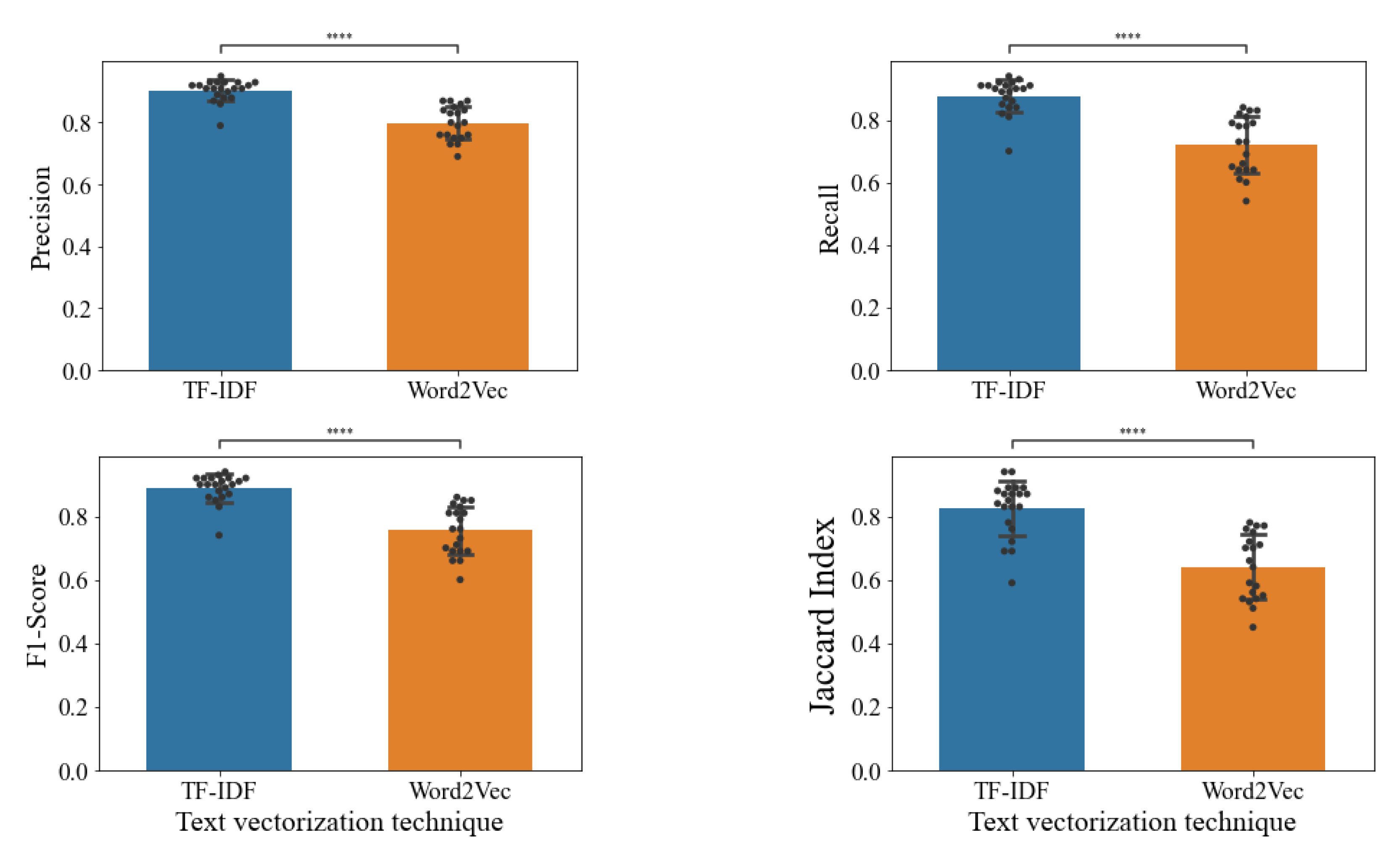
Later, using an SVM classifier, we had similar results in all metrics using the Logistic regression classifier (see
Figure 9). The Precision score yielded 0.9 ± 0.03 with TF-IDF, whereas Word2Vec had an average of 0.8 ± 0.05. The recall score with TF-IDF was 0.88 ± 0.05 against Word2Vec with an average of 0.73 ± 0.09. SVM F1-score reached 0.89 ± 0.04 with TF-IDF, whereas Word2Vec was 0.76 ± 0.07. Lastly, the Jaccard Index with TF-IDF reached an average of 0.82 ± 0.08, Word2Vec average score of 0.65 ± 0.1.
We only focused on results obtained with TF-IDF before clustering for further analysis. Next, we explored the impact of different stop lists over clustering and whether these clusters can be matched with a single movie genre.
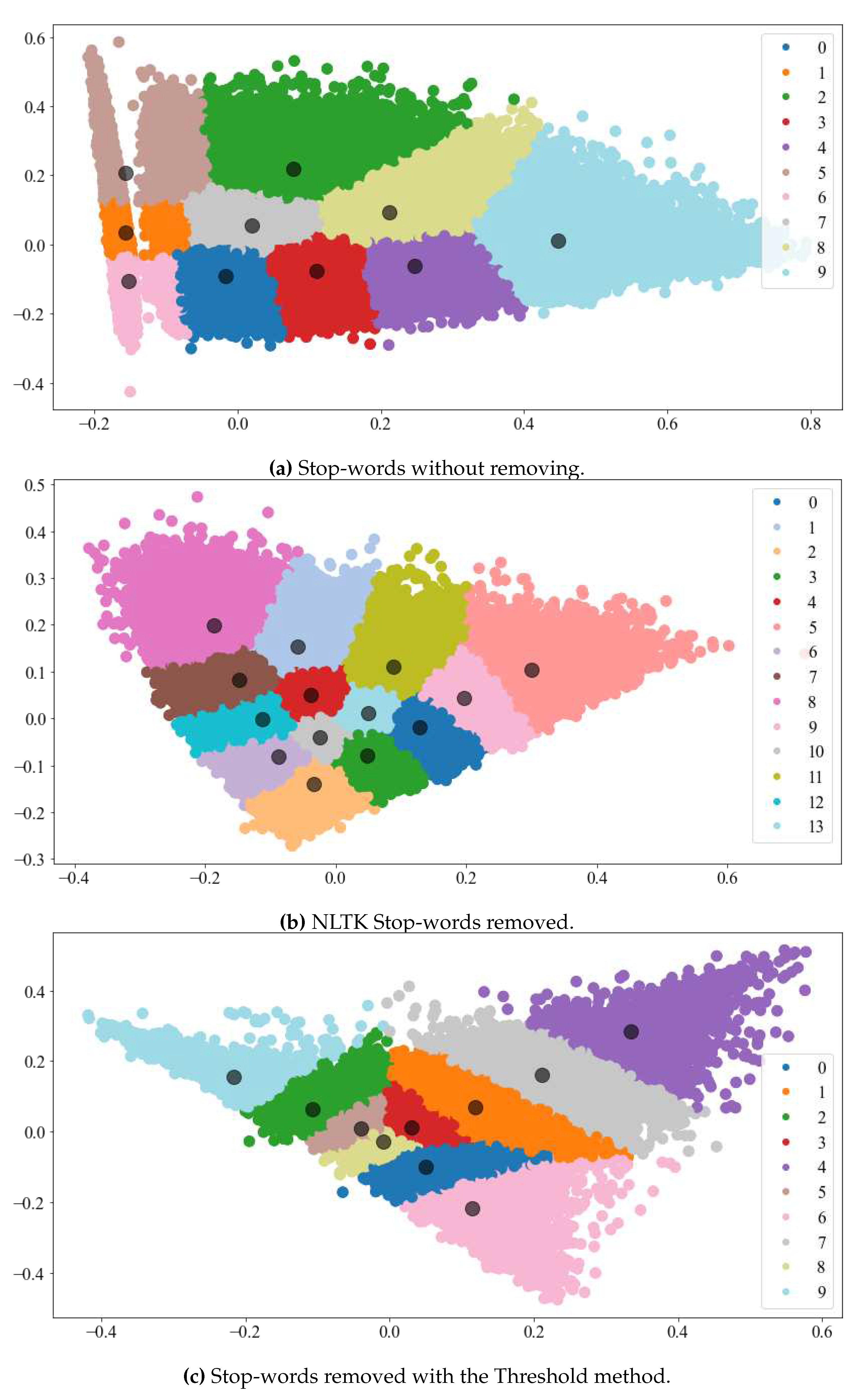
A secondary data preprocessing generated clusters with high ambiguity and poor separation between centroids. Whereas solely employing customized stop-lists resulted in better clustering visualization and featured similar to common movie genres (
Figure 10). The Top 10 features for each cluster in
Figure 10 are showed in
Table 7,
Table 8 and
Table 9.
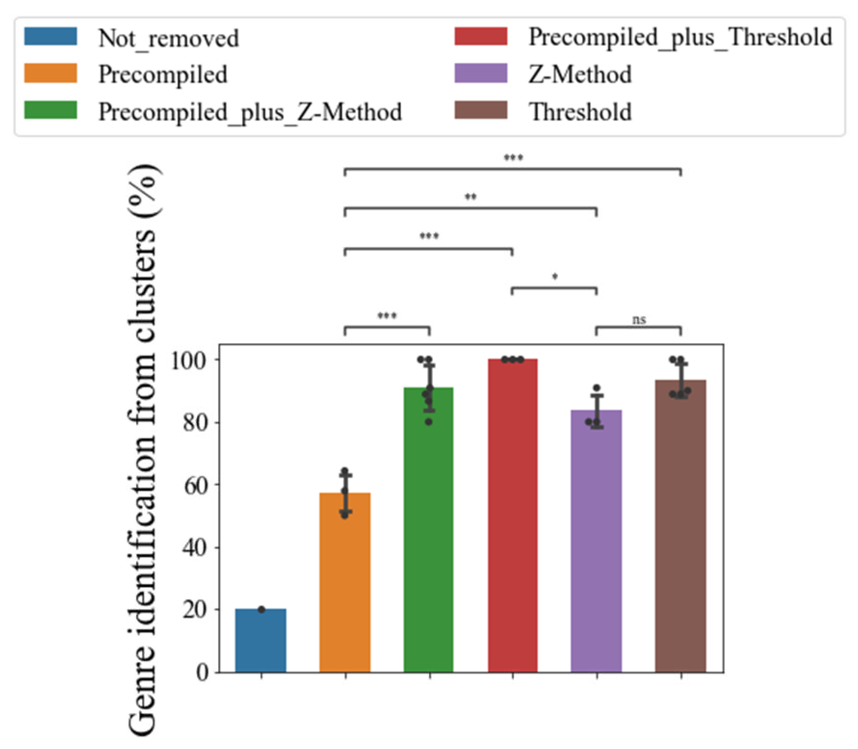
Furthermore, customized stop-word lists performed better than pre-compiled lists in generating clusters identifiable as movie genres (see
Figure 11). Overall, pre-compiled lists had an average of 57.39% ± 7.16 of genre prediction from clusters. Adding custom-generated stop-words with Z-Method yielded a 96.67% ± 8.16, and using the Threshold method, 94.74% ± 9.12. Finally, using only custom-generated stop-lists like Z-Method had an average of 86.67% ±11.55, whereas the Threshold method scored 79.46% ±13.26.
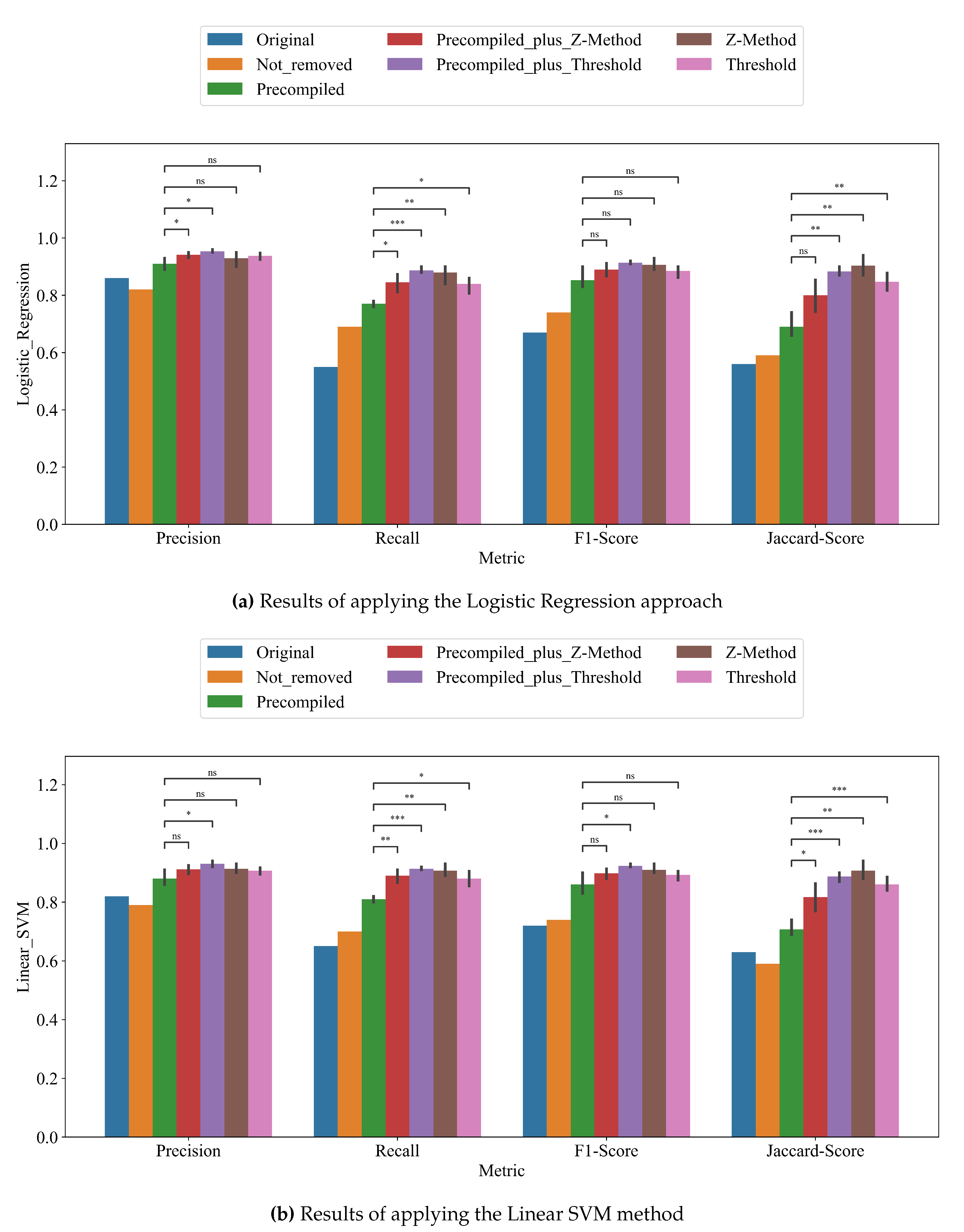
Finally, we tested the impact of the usage of different stop-word methods in the machine learning performance with the Logistic Regression approach (see
Figure 12a) and the Linear SVM method (see
Figure 12b). Globally, the sole use of custom stop-lists increased the precision metric and the Jaccard score index.
Notably, by looking at the classification reports, we observe significant differences between the various datasets (see
Table 10,
Table 11 and
Table 12). Not removing stop-words resulted in high heterogeneous scores between clusters regarding all metrics with numbers as low as 0.35 (see
Table 10, Cluster 5). By using pre-compiled lists such as NLTK, this effect improved, but it kept showing scores as low as 0.47 (see
Table 11, Cluster 10) and as high as 0.99 (see
Table 11, Cluster 9). Interestingly, using a method to create a customized stop-word list resulted in homogeneous scores; all cluster metrics drop between 0.72 (see
Table 12, Cluster 4) and 0.99 (see
Table 12, Cluster 2) even with classes with less support or data.
5. Discussion
The primary objective of this work was to test the effect of stop-words removal by different methods on unsupervised text classification using K-means clustering. Thus, the principal outcome was the clustered text that predicted the review genre. In this way, it allowed us to reclassify the reviews according to their content. The dataset was initially generated with web scrapping libraries from IMDb reviews by users. The reviews obtained the genre annotation from the movie without considering that as data generated by humans; thus, reviews are sparse and might only partially reflect the genres of the movie.
We have shown our data statements on the importance of text data pre-processing prior to unsupervised machine learning algorithms and how the clusters were grouped more precisely. Moreover, comparing different datasets generated by K-means clustering after using different stopword lists shows that, in most cases, it is statistically significant.
First, we tested the differences using two-word vector representations TF-IDF and Word2Vec. Both approaches were clustered and plotted with PCA in two dimensions using K-Means and the TF-IDF vector representation similarly to [
54]. Hence, TF-IDF showed a good cluster formation (see
Figure 5).
On the other hand, we experimented with the differences in Silhouette scores, number of clusters, clustering time, and the possibility of mapping a cluster with a specific movie genre. We found that using TF-IDF gave higher Silhouette scores, partially explaining why the clusters are well-defined. There was no difference in the average clusters or clustering time between vector representations. Regarding mapping a single cluster to a movie genre, TF-IDF proved more efficient for this task.
Finally, we sought to see the effect of the resulting relabeled datasets after clustering with well-known supervised machine learning algorithms such as Logistic Regression and SVM. Interestingly, the impact of using Word2Vec for word vector representation before clustering decreased performance compared to TF-IDF. For this specific task, using TF-IDF for vector representation results in better clustering formation, thus generating a balanced dataset for training and testing.
Moreover, we pushed the impact of using different methods to select and remove stop-words. We recommend removing the stop-words because it helps reduce data size and may improve the accuracy of models [
55]. Although it is empirically believed to affect sentiment analysis, in some cases, it is proven to have no effect at all [
56].
Generating custom stop lists is essential to avoid inherent biases and poor data cleaning; online tools are used to generate those lists [
57]. Here, we compared three pre-compiled stop-lists: NLTK from the Python toolkit project, that have 127 stop-words; ISO-en from a GitHub repository with 1,298 stop-words; and Genrec, which is a stop-list related to the movie domain with 720 stop-words. Using any of these pre-compiled lists resulted in poorly defined clusters that could not be assigned to a movie genre. Adding extra stop-words by Z-Method or our proposed method improved cluster definition and increased the genre prediction rate. Similarly, creating custom stop lists from scratch resulted in better genre prediction.
In addition, the effect on the machine learning performance demonstrated that using custom stop-lists instead of pre-compiled ones can improve the average precision and Jaccard index. Therefore, the classification report showed a better class balance without needing an enlargement data algorithm in classes with fewer data or reduction techniques in categories with more data than the others. In summary, a customized stop-word extraction before clustering improves the overall classification report regardless of the amount of data by class.
6. Conclusions
Reviewing the datasets we are working with before using them for later classifier training is highly recommended. The overwhelming data availability might offer a wide range of options to use as a corpus. Most of them are not curated, and labels might not be related to the text data shown. A solution is reclassifying this data using a clustering algorithm such as K-Means and its lighter version, Mini Batch K-Means.
We proposed an algorithm to identify stop-words (called the Threshold method). Datasets cleaned with our method or a hybrid version mixing pre-compiled stop lists such as NLTK showed better scores when using a machine learning classifier than a dataset without removing stop-words or using pre-compiled lists. Although we did not notice statistical differences between the Threshold method and the Z-method on classification metrics, The Threshold method performed better on the genre identification of clusters by its main features (see
Figure 11).
Interestingly, regarding the vectorization step before clustering with K-Means, TF-IDF worked better than Word2Vec for this task. It allowed us to detect the principal features by cluster; these words helped to detect the primary genre of the designated cluster, and then we could annotate it.
Thus, datasets can be reclassified using a similar protocol, avoiding curating them by hand or relying on sparse data with wrong labels. This protocol could be used to extract the main features of text data such as product reviews, tweets, or news and predict the labels, then be able to classify them.
Author Contributions
Conceptualization, F.G. and M.T.-R.; methodology, M.T.-R. and R.Q.; software, F.G. and G.R.-T.; validation, M.T.-R. and F.G.; formal analysis, F.G. and R.Q.; investigation, L.C. and G.R.-T.; resources, F.G. and G.R.-T.; data curation, M.T.-R. and R.Q.; writing—original draft preparation, F.G.; writing—review and editing, M.T.-R.; visualization, G.R.-T.; supervision, M.T.-R.; project administration, R.Q.; funding acquisition, L.C. All authors have read and agreed to the published version of the manuscript.
Funding
Work partially sponsored by Instituto Politécnico Nacional under grants 20230655 and 20230454. It also is sponsored by Consejo Nacional de Humanidades, Ciencias y Tecnologías (CONAHCYT), and Secretaría de Educación, Ciencia, Tecnología e Innovación (SECTEI).
Institutional Review Board Statement
Not applicable.
Informed Consent Statement
Not applicable.
Data Availability Statement
Not applicable
Acknowledgments
We are thankful to the reviewers for their invaluable and constructive feedback that helped improve the quality of this paper.
Conflicts of Interest
The authors declare no conflict of interest.
References
- Verma, P.; Gupta, P.; Singh, V. A Smart Movie Recommendation System Using Machine Learning Predictive Analysis. Proceedings of Data Analytics and Management: ICDAM 2022; 2023; pp. 45–56. [Google Scholar] [CrossRef]
- Lou, Y. Deep learning-based sentiment analysis of movie reviews. Third International Conference on Machine Learning and Computer Application (ICMLCA 2022). SPIE 2023, 12636, 177–184. [Google Scholar] [CrossRef]
- IMDb. IMDb datasets, 2022.
- Maas, A.L.; Daly, R.E.; Pham, P.T.; Huang, D.; Ng, A.Y.; Potts, C. Learning Word Vectors for Sentiment Analysis. Proceedings of the 49th Annual Meeting of the Association for Computational Linguistics: Human Language Technologies; Association for Computational Linguistics: Portland, Oregon, USA, 2011; pp. 142–150. [Google Scholar]
- Banik, R. The Movies Dataset, 2017.
- Lakshmi, P. IMDb Dataset of 50K Movie Reviews, 2019.
- Adinarayana, S.; Ilavarasan, E. A Hybrid Imbalanced Data Learning Framework to Tackle Opinion Imbalance in Movie Reviews. Communication Software and Networks; Satapathy, S.C., Bhateja, V., Ramakrishna Murty, M., Gia Nhu, N., Kotti, J., Eds.; Springer Singapore: Singapore, 2021; pp. 453–462. [Google Scholar] [CrossRef]
- Unal, F.Z.; Guzel, M.S.; Bostanci, E.; Acici, K.; Asuroglu, T. Multilabel Genre Prediction Using Deep-Learning Frameworks. Applied Sciences 2023, 13, 8665. [Google Scholar] [CrossRef]
- Battu, V.; Batchu, V.; Gangula, R.R.R.; Dakannagari, M.M.K.R.; Mamidi, R. Predicting the Genre and Rating of a Movie Based on its Synopsis. Proceedings of the 32nd Pacific Asia Conference on Language, Information and Computation; Association for Computational Linguistics: Hong Kong, 2018. [Google Scholar]
- wing Ho, K. Movies’ Genres Classification by Synopsis. Movies’ Genres Classification by Synopsis, 2011.
- Hoang, Q. Predicting Movie Genres Based on Plot Summaries, 2018. [CrossRef]
- Pal, A.; Barigidad, A.; Mustafi, A. Identifying movie genre compositions using neural networks and introducing GenRec-a recommender system based on audience genre perception. 2020 5th International Conference on Computing, Communication and Security (ICCCS), 2020; pp. 1–7. [Google Scholar] [CrossRef]
- Wissler, L.; Almashraee, M.; Monett, D.; Paschke, A. The Gold Standard in Corpus Annotation. 5th IEEE Germany Student Conference, 2014. [CrossRef]
- Zhang, X.; Zhao, J.; LeCun, Y. Character-level Convolutional Networks for Text Classification, 2015. [CrossRef]
- Lehmann, J.; Isele, R.; Jakob, M.; Jentzsch, A.; Kontokostas, D.; Mendes, P.; Hellmann, S.; Morsey, M.; Van Kleef, P.; Auer, S.; Bizer, C. DBpedia - A Large-scale, Multilingual Knowledge Base Extracted from Wikipedia. Semantic Web Journal 2014, 6. [Google Scholar] [CrossRef]
- Han, J.; Pei, J.; Tong, H. Data Mining: Concepts and Techniques; Elsevier Science, 2012. [Google Scholar]
- Arora, P.; Deepali; Varshney, S. Analysis of K-Means and K-Medoids Algorithm For Big Data. Procedia Computer Science 2016, 78, 507–512, 1st International Conference on Information Security & Privacy 2015. [Google Scholar] [CrossRef]
- Rose, R.L.; Puranik, T.G.; Mavris, D.N. Natural Language Processing Based Method for Clustering and Analysis of Aviation Safety Narratives. Aerospace 2020, 7. [Google Scholar] [CrossRef]
- Weißer, T.; Saßmannshausen, T.; Ohrndorf, D.; Burggräf, P.; Wagner, J. A clustering approach for topic filtering within systematic literature reviews. MethodsX 2020, 7, 100831. [Google Scholar] [CrossRef]
- Adinugroho, S.; Wihandika, R.C.; Adikara, P.P. Newsgroup topic extraction using term-cluster weighting and Pillar K-Means clustering. International Journal of Computers and Applications 2022, 44, 357–364. [Google Scholar] [CrossRef]
- Kumari, A.; Shashi, M. Vectorization of Text Documents for Identifying Unifiable News Articles. International Journal of Advanced Computer Science and Applications 2019, 10, 305. [Google Scholar] [CrossRef]
- Soni, R.; Mathai, K.J. Improved Twitter Sentiment Prediction through Cluster-then-Predict Model, 2015. [CrossRef]
- Zhao, Y. R and Data Mining: Examples and Case Studies; Elsevier, 2012. [Google Scholar]
- Kaur, N. A Combinatorial Tweet Clustering Methodology Utilizing Inter and Intra Cosine Similarity. PhD thesis, Faculty Of Graduate Studies And Research, University Of Regina, 2015. [Google Scholar]
- Miyamoto, S.; Suzuki, S.; Takumi, S. Clustering in tweets using a fuzzy neighborhood model. 2012 IEEE International Conference on Fuzzy Systems, 2012; pp. 1–6. [Google Scholar] [CrossRef]
- Kadhim, A.I.; Cheah, Y.N.; Ahamed, N.H. Text Document Preprocessing and Dimension Reduction Techniques for Text Document Clustering. 2014 4th International Conference on Artificial Intelligence with Applications in Engineering and Technology, 2014; pp. 69–73. [Google Scholar] [CrossRef]
- Fodeh, S.J.; Al-Garadi, M.; Elsankary, O.; Perrone, J.; Becker, W.; Sarker, A. Utilizing a multi-class classification approach to detect therapeutic and recreational misuse of opioids on Twitter. Computers in Biology and Medicine 2021, 129, 104132. [Google Scholar] [CrossRef]
- Bird, S.; Loper, E. NLTK: The Natural Language Toolkit. Proceedings of the ACL Interactive Poster and Demonstration Sessions; Association for Computational Linguistics: Barcelona, Spain, 2004; pp. 214–217. [Google Scholar] [CrossRef]
- Gene, D.; Suriyawongkul, A. stopwords-iso. Github, 2020.
- Piantadosi, S.T. Zipf’s word frequency law in natural language: A critical review and future directions. Psychonomic Bulletin & Review 2014, 21, 1112–1130. [Google Scholar] [CrossRef]
- Rajaraman, A.; Ullman, J.D. Data Mining. In Mining of Massive Datasets; Cambridge University Press, 2011; pp. 1–17. [Google Scholar] [CrossRef]
- Mikolov, T.; Chen, K.; Corrado, G.; Dean, J. Efficient Estimation of Word Representations in Vector Space, 2013. [CrossRef]
- Blashfield, R.K.; Aldenderfer, M.S. The Literature On Cluster Analysis. Multivariate Behavioral Research 1978, 13, 271–295. [Google Scholar] [CrossRef] [PubMed]
- Wei, D.; Jiang, Q.; Wei, Y.; Wang, S. A novel hierarchical clustering algorithm for gene sequences. BMC Bioinformatics 2012, 13, 174. [Google Scholar] [CrossRef] [PubMed]
- Filipovych, R.; Resnick, S.M.; Davatzikos, C. Semi-supervised cluster analysis of imaging data. NeuroImage 2011, 54, 2185–2197. [Google Scholar] [CrossRef] [PubMed]
- Punj, G.; Stewart, D.W. Cluster Analysis in Marketing Research: Review and Suggestions for Application. Journal of Marketing Research 1983, 20, 134–148. [Google Scholar] [CrossRef]
- Cooley, R.; Mobasher, B.; Srivastava, J. Data Preparation for Mining World Wide Web Browsing Patterns. Knowledge and Information Systems 1999, 1, 5–32. [Google Scholar] [CrossRef]
- Fonseca, J.R. Clustering in the field of social sciences: That is your choice. International Journal of Social Research Methodology 2013, 16, 403–428. [Google Scholar] [CrossRef]
- Dhanachandra, N.; Manglem, K.; Chanu, Y.J. Image Segmentation Using K -means Clustering Algorithm and Subtractive Clustering Algorithm. Procedia Computer Science 2015, 54, 764–771. [Google Scholar] [CrossRef]
- Fahad, A.; Alshatri, N.; Tari, Z.; Alamri, A.; Khalil, I.; Zomaya, A.Y.; Foufou, S.; Bouras, A. A Survey of Clustering Algorithms for Big Data: Taxonomy and Empirical Analysis. IEEE Transactions on Emerging Topics in Computing 2014, 2, 267–279. [Google Scholar] [CrossRef]
- Gallardo Garcia, R.; Beltran, B.; Vilariño, D.; Zepeda, C.; Martínez, R. Comparison of Clustering Algorithms in Text Clustering Tasks. Computacion y Sistemas 2020, 24. [Google Scholar] [CrossRef]
- Hadifar, A.; Sterckx, L.; Demeester, T.; Develder, C. A Self-Training Approach for Short Text Clustering". Proceedings of the 4th Workshop on Representation Learning for NLP (RepL4NLP-2019); Association for Computational Linguistics: Florence, Italy, 2019; pp. 194–199. [Google Scholar] [CrossRef]
- Naeem, S.; Wumaier, A. Study and Implementing K-mean Clustering Algorithm on English Text and Techniques to Find the Optimal Value of K. International Journal of Computer Applications 2018, 182, 7–14. [Google Scholar] [CrossRef]
- Tou, J.; Gonzalez, R.C. Pattern recognition principles; Addison-Wesley Publishing Company, 1974. [Google Scholar]
- Sculley, D. Web-Scale k-Means Clustering. Proceedings of the 19th International Conference on World Wide Web; Association for Computing Machinery: New York, NY, USA, 2010. [Google Scholar] [CrossRef]
- Thorndike, R.L. Who belongs in the family? Psychometrika 1953, 18, 267–276. [Google Scholar] [CrossRef]
- Rousseeuw, P.J. Silhouettes: A graphical aid to the interpretation and validation of cluster analysis. Journal of Computational and Applied Mathematics 1987, 20, 53–65. [Google Scholar] [CrossRef]
- Caliński, T.; Harabasz, J. A dendrite method for cluster analysis. Communications in Statistics 1974, 3, 1–27. [Google Scholar] [CrossRef]
- Shahapure, K.R.; Nicholas, C. Cluster Quality Analysis Using Silhouette Score. 2020 IEEE 7th International Conference on Data Science and Advanced Analytics (DSAA), 2020; pp. 747–748. [Google Scholar] [CrossRef]
- Tixier, A.J.P. Notes on deep learning for nlp. arXiv 2018. [Google Scholar]
- Franc, V.; Zien, A.; Schölkopf, B. Support vector machines as probabilistic models. ICML, 2011.
- N., V.V. Adaptive and Learning Systems for Signal Processing Communications, and control. Statistical Learning Theory 1998.
- Wei, Q.; Dunbrack, R.L., Jr. The Role of Balanced Training and Testing Data Sets for Binary Classifiers in Bioinformatics. PLOS ONE 2013, 8, 1–12. [Google Scholar] [CrossRef]
- Rostom, E. Unsupervised Clustering and Multi-Label Classification of Ticket Data. Master’s thesis, Freie Universitat Berlin, 2018. [Google Scholar]
- Saif, H.; Fernandez, M.; He, Y.; Alani, H. On Stopwords, Filtering and Data Sparsity for Sentiment Analysis of Twitter. Proceedings of the Ninth International Conference on Language Resources and Evaluation (LREC’14); European Language Resources Association (ELRA): Reykjavik, Iceland, 2014; pp. 810–817. [Google Scholar]
- Ghag, K.V.; Shah, K. Comparative analysis of effect of stopwords removal on sentiment classification. 2015 International Conference on Computer, Communication and Control (IC4), 2015; pp. 1–6. [Google Scholar] [CrossRef]
- Blanchard, A. Understanding and customizing stopword lists for enhanced patent mapping. World Patent Information 2007, 29, 308–316. [Google Scholar] [CrossRef]
Figure 1.
Methodology for classification and visualization of movie user reviews. User reviews from top movies browsed by genre retrieved through web scrapping from IMDb.com.
Figure 1.
Methodology for classification and visualization of movie user reviews. User reviews from top movies browsed by genre retrieved through web scrapping from IMDb.com.
Figure 2.
Silhouette Score. Data showed is the mean ± standard deviation. Statistical analysis is a t-test for independent samples. p-val<0.001:***
Figure 2.
Silhouette Score. Data showed is the mean ± standard deviation. Statistical analysis is a t-test for independent samples. p-val<0.001:***
Figure 3.
Silhouette scores after cleaning with the Threshold method. Dotted lines represent the dataset without removed stop-words (Not_removed), and solid lines show scores of the dataset without stop-words (Threshold method), both later tokenized with TF-IDF (blue) or embedded with Word2vec (red) prior clustering.
Figure 4.
The best number of clusters. Data showed is the mean ± standard deviation. Statistical analysis is a t-test for independent samples. p-val<0.01:**
Figure 4.
The best number of clusters. Data showed is the mean ± standard deviation. Statistical analysis is a t-test for independent samples. p-val<0.01:**
Figure 5.
The PCA plotting of dimensionally reduced data comparing TF-IDF vs. Word2Vec. In this example, we can notice the clustering representation of the datasets cleaned with NLTK stopword lists and vectorized with TF-IDF (a) or Word2Vec (b)
Figure 5.
The PCA plotting of dimensionally reduced data comparing TF-IDF vs. Word2Vec. In this example, we can notice the clustering representation of the datasets cleaned with NLTK stopword lists and vectorized with TF-IDF (a) or Word2Vec (b)
Figure 6.
Clustering time. Data showed is the mean ± standard deviation. Statistical analysis is a t-test for independent samples. p-val>0.05: ns.
Figure 6.
Clustering time. Data showed is the mean ± standard deviation. Statistical analysis is a t-test for independent samples. p-val>0.05: ns.
Figure 7.
Clusters corresponding to a movie genre. Data showed is the mean ± standard deviation. Statistical analysis is a t-test for independent samples. p-val<0.0001: ****
Figure 7.
Clusters corresponding to a movie genre. Data showed is the mean ± standard deviation. Statistical analysis is a t-test for independent samples. p-val<0.0001: ****
Figure 8.
Logistic Regression results comparing TF-DF vs. Word2Vec. All different datasets were cleaned as showed before, tokenized with TF-IDF, or embedded with Word2Vec prior clustering algorithm. Generated datasets were trained and tested with the Linear SVM. Data showed is the mean ± standard deviation. Statistical analysis is a t-test for independent samples. p-val<0.0001:****
Figure 9.
Linear SVM results comparing TF-DF vs. Word2Vec. All different datasets were cleaned as showed before, tokenized with TF-IDF, or embedded with Word2Vec prior clustering algorithm. Generated datasets were trained and tested with the Linear SVM. Data showed is the mean ± standard deviation. Statistical analysis is a t-test for independent samples. p-val<0.0001:****
Figure 10.
Cluster distribution with two dimension PCA.
Figure 10.
Cluster distribution with two dimension PCA.
Figure 11.
Clusters corresponding to a movie genre improved with custom stop-words lists. Clusters with word collections related to a genre were marked with the most similar genre, whereas clusters with gibberish were identified as undefined. Data showed is the mean ± standard deviation. Statistical analysis is a t-test for independent samples. p-val<0.05: *, p-val<0.01: **, p-val<0.001: ***
Figure 12.
Comparison of different datasets generated by K-Means clustering after using different stopword lists. Data is the mean ± SEM, statistical test corresponds to t-test independent samples, p-val<0.05: *, p-val<0.01: **.
Figure 12.
Comparison of different datasets generated by K-Means clustering after using different stopword lists. Data is the mean ± SEM, statistical test corresponds to t-test independent samples, p-val<0.05: *, p-val<0.01: **.
Table 1.
Removal methods for stop-words
Table 1.
Removal methods for stop-words
| Method |
Description |
| Baseline |
The baseline method of this study is the non-removal of stop-words. We preprocessed the original dataset as described before, but non-stopwords were removed. |
| Classic method: Pre-compiled stop-words lists |
In this study, we employed three different stop-words lists: NLTK [28], ISO-en [29], and the list generated by [12] referred to as Genrec. |
| Method based on Zipf’s law: Z-Method |
There are many different methods to compute custom stoplists for various languages. The most common ones are based on Zipf’s law [30]. In this method, the frequency of each distinct word in the text is calculated, and then the words are sorted in decreasing order of their frequencies. Then, the top k most frequent words are added to a stopword list and removed from the text. |
| Proposed method: Threshold |
The proposed method verifies if a proposed stop-word is present in each review across all genres; if this condition is met, then checks if the frequency of the word is at least a designated threshold (see Algorithm 1 below). |
| Combined stop-words list |
Datasets were cleaned with the list of stop-words mentioned above, and then either with the Z-Method or Threshold method or custom stop-words were detected and removed. |
Table 2.
Types of clustering algorithms
Table 2.
Types of clustering algorithms
| Clustering Algorithm Type |
Description |
Examples |
| Partitioning-Based |
The number of groups is determined in the beginning. Then, the partitioning algorithms divide data objects into many partitions, each representing a cluster. |
K-means, K-mediods, K-modes, PAM, CLARA, CLARANS and FCM. |
| Hierarchical-Based |
Data are organized hierarchically depending on the medium of proximity. The intermediate nodes obtain proximities. A dendrogram represents the datasets, where leaf nodes present individual data. |
BIRCH, CURE, ROCK and Chameleon |
| Density-Based |
Data objects are separated based on density, connectivity, and boundary regions. They are closely related to point-nearest neighbors. A cluster, defined as a connected dense component, grows in any direction that density leads. |
DBSCAN, OPTICS, DBCLASD and DENCLUE |
| Grid-Based |
Grid-based clustering algorithms partition the data space into a finite number of cells to form a grid structure and then form clusters from the cells in the grid structure. |
Wave-Cluster and STING |
| Model-Based |
Such a method optimizes the fit between the given data and some (predefined) mathematical models. It is based on the assumption that a mixture of underlying probability distributions generates the data. Also, it automatically determines the number of clusters based on standard statistics, taking noise (outliers) into account and thus yielding a robust clustering method. |
MCLUST and COBWEB |
Table 3.
Original dataset
Table 3.
Original dataset
| Genre |
Reviews |
| Biography |
33,295 |
| History |
24,397 |
| Action |
28,723 |
| Drama |
36,565 |
| Horror |
20,477 |
| Comedy |
31,181 |
| Romance |
24,671 |
| Adventure |
25,048 |
| Crime |
24,557 |
| Mystery |
16,033 |
| Sci-Fi |
13,985 |
| Thriller |
23,646 |
| Fantasy |
13,982 |
| War |
19,111 |
| Music |
20,814 |
| Western |
19,293 |
| Sport |
18,129 |
| Animation |
24,530 |
| Total |
418,437 |
Table 4.
Characteristics of the datasets
Table 4.
Characteristics of the datasets
| Datasets |
Number |
Pre-Compiled List |
Custom List |
Total Stopwords |
| Original |
1 |
NA |
NA |
0 |
| Not_removed |
1 |
NA |
NA |
0 |
| NLTK |
1 |
127 |
0 |
127 |
| NTLK + Z-Method |
2 |
127 |
50-98 |
177-225 |
| ISO |
1 |
1,298 |
0 |
1,298 |
| ISO + Z-Method |
2 |
1,298 |
47-89 |
1,345-1,387 |
| ISO + Threshold |
3 |
1,298 |
167-412 |
1,465-1,710 |
| Genrec |
1 |
720 |
0 |
720 |
| Genrec + Z-Method |
2 |
720 |
48-91 |
768-811 |
| Z-Method |
3 |
NA |
288-985 |
288-985 |
| Threshold |
8 |
NA |
160-1,346 |
160-1,346 |
| Total |
25 |
|
|
|
Table 5.
TF-IDF - Top 10 features by cluster.
Table 5.
TF-IDF - Top 10 features by cluster.
| Cluster |
Top 10 Features |
Genre |
| 0 |
horror, film, movi, horror film, horror movi, like, scare, scari, origin,good |
Horror |
| 1 |
comedi, funni, movi, laugh, film, joke, like, good, time, make, |
Comedy |
| 2 |
film, like, charact, stori, time, good, make, watch, realli, scene, |
Undefined |
| 3 |
music, danc, song, movi, film, sing, love, like, stori, great |
Music |
| 4 |
anim, disney, film, movi, voic, charact, stori, like, kid, good |
Animation |
| 5 |
film, life, movi, stori, play, man, time, make, love, famili |
Undefined |
| 6 |
western, film, eastwood, movi, west, good, town, charact, great, time, |
Western |
| 7 |
war, film, movi, soldier, german, battl, stori, scene, american, like, |
War |
| 8 |
wayn, john, western, ford, film, movi, charact, play, great, indian |
Western |
| 9 |
rocki, fight, movi, film, box, train, like, good, son, seri |
Sport |
| 10 |
movi, like, realli, film, good, charact, stori, time, thing, make |
Undefined |
| 11 |
movi, watch, like, good, realli, great, stori, time, charact, make |
Undefined |
| 12 |
film, perform, best, stori, role, movi, oscar, actor, great, play |
Undefined |
| 13 |
action, film, movi, good, scene, charact, like, time, plot, sequenc, |
Action |
Table 6.
Word2vec - Top 10 features by cluster.
Table 6.
Word2vec - Top 10 features by cluster.
| Cluster |
Top 10 Features |
Genre |
| 0 |
movi, realli, film, think, definit, great, good, sure, honestli, certainli |
Undefined |
| 1 |
go, happen, want, know, get, find, decid, peopl, thing, actual |
Undefined |
| 2 |
movi, realli, think, sure, actual, honestli, lot, good, enjoy, said |
Undefined |
| 3 |
film, movi, howev, realli, think, feel, simpli, actual, stori, mani |
Undefined |
| 4 |
peopl, movi, film, actual, think, howev, fact, one, understand, therefor |
Undefined |
| 5 |
film, movi, realli, think, one, sure, actual, certainli, howev, great |
Undefined |
| 6 |
think, realli, movi, actual, sure, know, anyway, honestli, guess, kind |
Undefined |
| 7 |
movi, think, realli, actual, sure, know, thing, one, said, anyway |
Undefined |
| 8 |
movi, realli, film, think, actual, sure, much, howev, lot, overal |
Undefined |
| 9 |
think, movi, realli, way, actual, understand, know, howev, peopl, one |
Undefined |
| 10 |
movi, realli, film, think, sure, still, actual, enjoy, one, definit |
Undefined |
| 11 |
movi, think, realli, film, actual, sure, one, said, howev, know |
Undefined |
| 12 |
movi, realli, actual, think, film, sure, howev, one, thing, much |
Undefined |
| 13 |
movi, think, realli, sure, actual, film, watch, honestli, said, definit |
Undefined |
Table 7.
Stop-words without removing
Table 7.
Stop-words without removing
| Cluster |
Top 10 Features |
Genre |
| 0 |
hi, br, thi, film, ha, life, movi, br br, wa, play |
Undefined |
| 1 |
br, movi, br br, thi, wa, thi movi, like, good, watch, just |
Undefined |
| 2 |
movi, thi, thi movi, wa, watch, like, good, just, great, realli |
Undefined |
| 3 |
war, br, film, movi, thi, soldier, wa, br br, german, hi |
War |
| 4 |
film, thi, thi film, br, wa, veri, like, br br, good, watch |
Undefined |
| 5 |
br, br br, film, thi, hi, wa, stori, ha, movi, like |
Undefined |
| 6 |
wa, movi, thi, did, br, film, like, good, just, veri |
Undefined |
| 7 |
anim, br, disney, film, thi, movi, voic, br br, wa, stori |
Animation |
| 8 |
br, br br, thi, wa, film, movi, hi, like, good, stori |
Undefined |
| 9 |
thi, film, movi, stori, good, ha, like, wa, time, charact |
Undefined |
Table 8.
NLTK Stop-words removed
Table 8.
NLTK Stop-words removed
| Cluster |
Top 10 features |
Genre |
| Cluster 0 |
horror, film, movi, horror film, horror movi, like, scare, scari |
Horror |
| Cluster 1 |
comedi, funni, movi, laugh, film, joke, like, good, time, make |
Comedy |
| Cluster 2 |
film, like, charact, stori, time, good, make, watch, realli, scene |
Undefined |
| Cluster 3 |
music, danc, song, movi, film, sing, love, like, stori, great |
Musical |
| Cluster 4 |
anim, disney, film, movi, voic, charact, stori, like, kid, good |
Animation |
| Cluster 5 |
film, life, movi, stori, play, man, time, make, love, famili |
Undefined |
| Cluster 6 |
western, film, eastwood, movi, west, good, town, charact, great, time |
Western |
| Cluster 7 |
war, film, movi, soldier, german, battl, stori, scene, american, like |
War |
| Cluster 8 |
wayn, john, western, ford, film, movi, charact, play, great, indian |
Western |
| Cluster 9 |
rocki, fight, movi, film, box, train, like, good, son, seri |
Sport |
| Cluster 10 |
movi, like, realli, film, good, charact, stori, time, thing, make, |
Undefined |
| Cluster 11 |
movi, watch, like, good, realli, great, stori, time, charact, make |
Undefined |
| Cluster 12 |
film, perform, best, stori, role, movi, oscar, actor, great, play |
Undefined |
| Cluster 13 |
action, film, movi, good, scene, charact, like, time, plot, sequenc |
Action |
Table 9.
Stop-words removed with the Threshold method.
Table 9.
Stop-words removed with the Threshold method.
| Cluster |
Top 10 Features |
Genre |
| 0 |
horror, scari, scare, gore, genr, dead, creepi, hous, zombi, remak |
Horror |
| 1 |
war, soldier, german, battl, american, men, fight, action, histori, privat |
War |
| 2 |
rocki, fight, box, train, seri, son, franchis, sequel, ring, match |
Sport |
| 3 |
western, wayn, eastwood, west, clint, town, ford, genr, stewart, indian |
Western |
| 4 |
kid, adult, child, famili, fun, anim, parent, funni, school, voic |
Family |
| 5 |
famili, book, base, power, girl, human, portray, drama, american, oscar |
Drama |
| 6 |
anim, disney, voic, song, child, famili, fun, music, featur, kid |
Animation |
| 7 |
funni, comedi, laugh, joke, hilari, humor, fun, sandler, romant, stupid |
Comedy |
| 8 |
music, danc, song, sing, rock, band, singer, soundtrack, number, girl |
Music |
| 9 |
action, sequenc, fight, fun, action sequenc, seri, sequel, special, kill, hero |
Action |
Table 10.
Classification report without removing stop-words
Table 10.
Classification report without removing stop-words
| |
Precision |
Recall |
F1-score |
Support |
| Cluster 0 |
0.86 |
0.72 |
0.78 |
4,548 |
| Cluster 1 |
0.65 |
0.37 |
0.47 |
6,137 |
| Cluster 2 |
0.87 |
0.77 |
0.82 |
6,028 |
| Cluster 3 |
0.91 |
0.78 |
0.84 |
1,762 |
| Cluster 4 |
0.86 |
0.74 |
0.79 |
5,576 |
| Cluster 5 |
0.58 |
0.35 |
0.44 |
10,823 |
| Cluster 6 |
0.85 |
0.69 |
0.76 |
4,819 |
| Cluster 7 |
0.9 |
0.81 |
0.86 |
2,130 |
| Cluster 8 |
0.92 |
0.84 |
0.88 |
5,105 |
| Cluster 9 |
0.83 |
0.78 |
0.8 |
12,541 |
| micro avg |
0.81 |
0.65 |
0.72 |
59,469 |
| macro avg |
0.82 |
0.69 |
0.74 |
59,469 |
| weighted avg |
0.79 |
0.65 |
0.71 |
59,469 |
| samples avg |
0.59 |
0.65 |
0.61 |
59,469 |
Table 11.
Classification report removing NLTK stop-words
Table 11.
Classification report removing NLTK stop-words
| |
Precision |
Recall |
F1-score |
Support |
| Cluster 0 |
0.93 |
0.84 |
0.88 |
2,463 |
| Cluster 1 |
0.89 |
0.78 |
0.83 |
3,681 |
| Cluster 2 |
0.88 |
0.77 |
0.82 |
8,735 |
| Cluster 3 |
0.92 |
0.79 |
0.85 |
2,346 |
| Cluster 4 |
0.95 |
0.89 |
0.92 |
3,061 |
| Cluster 5 |
0.82 |
0.74 |
0.77 |
12,140 |
| Cluster 6 |
0.93 |
0.82 |
0.87 |
1,625 |
| Cluster 7 |
0.94 |
0.85 |
0.9 |
2,660 |
| Cluster 8 |
0.97 |
0.83 |
0.9 |
501 |
| Cluster 9 |
0.99 |
0.91 |
0.95 |
396 |
| Cluster 10 |
0.72 |
0.47 |
0.57 |
9,496 |
| Cluster 11 |
0.9 |
0.82 |
0.86 |
7,444 |
| Cluster 12 |
0.81 |
0.59 |
0.68 |
5,798 |
| Cluster 13 |
0.87 |
0.69 |
0.77 |
3,640 |
| micro avg |
0.86 |
0.72 |
0.78 |
63,986 |
| macro avg |
0.89 |
0.77 |
0.83 |
63,986 |
| weighted avg |
0.85 |
0.72 |
0.78 |
63,986 |
| samples avg |
0.67 |
0.72 |
0.69 |
63,986 |
Table 12.
Classification report with the Threshold method
Table 12.
Classification report with the Threshold method
| |
Precision |
Recall |
F1-score |
Support |
| Cluster 0 |
0.96 |
0.88 |
0.92 |
2,695 |
| Cluster 1 |
0.96 |
0.88 |
0.92 |
3,122 |
| Cluster 2 |
0.99 |
0.9 |
0.94 |
368 |
| Cluster 3 |
0.96 |
0.89 |
0.92 |
2,045 |
| Cluster 4 |
0.92 |
0.72 |
0.81 |
2,382 |
| Cluster 5 |
0.92 |
0.94 |
0.93 |
32,226 |
| Cluster 6 |
0.95 |
0.9 |
0.92 |
3,076 |
| Cluster 7 |
0.95 |
0.86 |
0.9 |
5,045 |
| Cluster 8 |
0.95 |
0.83 |
0.89 |
3,752 |
| Cluster 9 |
0.92 |
0.83 |
0.88 |
4,757 |
| micro avg |
0.93 |
0.9 |
0.92 |
59,468 |
| macro avg |
0.95 |
0.85 |
0.9 |
59,468 |
| weighted avg |
0.93 |
0.9 |
0.92 |
59,468 |
| samples avg |
0.88 |
0.9 |
0.89 |
59,468 |
|
Disclaimer/Publisher’s Note: The statements, opinions and data contained in all publications are solely those of the individual author(s) and contributor(s) and not of MDPI and/or the editor(s). MDPI and/or the editor(s) disclaim responsibility for any injury to people or property resulting from any ideas, methods, instructions or products referred to in the content. |
© 2023 by the authors. Licensee MDPI, Basel, Switzerland. This article is an open access article distributed under the terms and conditions of the Creative Commons Attribution (CC BY) license (http://creativecommons.org/licenses/by/4.0/).
