1. Introduction
Any neighbour tissue impairment due to uncontrolled cell growth and its invasion is called as Cancer. Oral cancer is ranked sixth most prevailing cancer globally and it falls under the broad category of head and neck cancer. Oral cancer results in malignant cancer cell growth in lips and various parts of oral cavity. Worldwide, it is ranked as the fifteenth most common reason for death among various types of cancer. Out of one lakh people, minimum four people are affected by this disease across the globe [
1,
2]. Approximately, seventy-seven new cases and fifty-two thousand deaths are registered every year in India and one-fourth of the global oral cancer occurs in India [
3].
Most common types of oral cancer include Oral Squamous Cell Carcinoma (OSCC), Verrucous carcinoma, Minor salivary gland carcinomas, Lymphoma, and Mucosal melanoma. Among them, OSCC is a predominant type of oral cancer which contributes around 84% – 97% of oral cancer [
4]. The major risk factors that lead to development of OSCC includes tobacco usage, frequent chewing of betel quid, alcohol intake, oral infection, and genetic disorders [
5]. Detection of OSCC at early stage is very crucial to avoid deaths since the five-year survival rate of humans with early-stage OSCC is around 85% while it is only around 40% with advanced stage [
6,
7]. Hence early detection is the key to reduce the mortality rate and so there is a huge demand for diagnostic tools that identifies the OSCC at earlier stages of malignancy.
Apart from physical examination, major diagnostic tools used for identification of oral cancer includes techniques such as endoscope biopsy, liquid biopsy, vital staining technique, ultrasound imaging, Magnetic Resonance Imaging (MRI), Computed Tomography (CT) imaging, Raman spectroscopy, Gene/DNA array-based biomarker detection, enzyme assays-based biomarker detection, and histopathological examination [
4]. Among these techniques, histopathologic examination is mainly preferred since it can be used to detect both malignant and benign tumours by identifying the changes in histopathological and molecular levels. Histological assays can be used to reveal the gradual growth of malignant cells in oral cavity beginning from elementary dysplasia to tumours with high invasive nature. It is helpful in analysing the cells proliferation, growth of abnormalities, cytoplasmic-level and cellular-level atypia, changes at the surface of epithelium, and deep tissue-level cytoarchitecture [
8]. Usually, abnormalities in microscopic and clinical levels arise only after the abnormalities in molecular and genetic levels. Histopathological examination is good in capturing these molecular level changes and so preferred for early detection [
9].
Analysis of histopathological images through visual inspection is usually subjective in nature and prone to errors sometimes. Computerized diagnostic tools will be very helpful to assist the clinician in the decision-making process to reduce such errors. Various Machine Learning (ML) techniques are used nowadays in variety of fields. Particularly in healthcare field, the implementation of ML algorithms is increasing day by day. Accuracy and robustness are the key concerns in such healthcare related decision-making tools. Fortunately, nowadays Deep Learning (DL) models are available for solving these issues. Deep learning is a sub-field in machine learning where the Artificial Neural Network (ANN) models with many numbers hidden layers are trained with large set of training images and labels; labels of new unseen images will be predicted using the trained model. The main advantage of deep learning is the non-requirement of hand-crafted feature engineering compared to traditional supervised classifiers such as Support Vector Machine (SVM), K-Nearest Neighbour (KNN), Decision Trees (DT), etc where domain experts are required to identify the appropriate features and Region of Interest (RoI) [
10,
11].
Convolutional Neural Network (CNN) is a popular deep learning technique where convolution operation is involved in multiple ANN layers. Various CNN architectures are developed, and they are very efficient in different image classification tasks [
12,
13]. Popular CNN architectures include ResNet, EffiecientNet, InceptionNet, MobileNet, etc. The main advantage of these architectures is their ability to work well on a classification task even if most of their weights are pre-trained on another classification task. This concept is known as transfer learning and works very well for two similar and unique classification tasks. Two main advantages of transfer learning are reduction in training time and competence to work well on small datasets [
14,
15].
To improve the accuracy of such deep learning models, various techniques are used such as fine-tuning, feature selection, regularization, optimal parameter selection, optimization, etc. On the other hand, various population-based Swarm Intelligence (SI) optimization algorithms are widely used for optimal parameter identification, weights updating and feature selection in deep learning models for enhancing the accuracy. SI algorithms are meta-heuristic iterative algorithm that are usually inspired by the characteristic and nature of Swarm of animals. These algorithms are preferred in many applications mainly due to their minimalism, derivation free design and ability to avoid local optima [
16]. Some of the popular SI algorithms include Particle Swarm Optimization (PSO), Ant Colony Optimization, Grey Wolf Optimizer, Dragonfly Optimization, Elephant Herding Optimization, Gorilla Troops Optimizer (GTO), etc.
This work primarily focuses on classifying the histopathological images into two categories: Normal and OSCC. Histopathological image features are extracted using pre-trained weights of transfer learning based popular CNN models namely InceptionV2, MobileNetV3, and EfficientNetB3. Then Modified Gorilla Troops Optimizer (MGTO) is used as an intermediate layer in between feature extraction and classification layers. Two fully connected ANN layers along with batch normalization and dropout are used as classification layers.
The key contributions of this research work are listed below:
Proposal of novel deep learning framework that includes a swarm intelligence-based optimization algorithm as an intermediate layer in deep learning model.
Development of MGTO through appropriate modifications that enhances the classification accuracy.
Comparative analysis of popular deep learning models with and without the proposed intermediate layer in terms of various classification metrics and training time.
The remaining paper is organized as follows:
Section 2 deals with the related works and section 3 is related to background of various transfer learning models used and original GTO. Fourth section deals with the methodology used in this research work and fifth section presents the implementation procedure for proposed MGTO as an intermediate layer. Results are presented and discussed in the sixth section. Last section summarizes the conclusion and future work.
2. Related work
Various techniques based on machine learning and deep learning are proposed in the literature to diagnose oral cancer by analysing the medical images. Early publication related to oral cancer diagnosis mainly revolves around feature extraction and traditional supervised classifiers [17-20]. For example, [
21] considered features based on texture discrimination using higher order spectra, laws texture energy, and local binary pattern and fed these features to supervised classifiers such as DT, Gaussian Mixture Mode, KNN, Sugeno Fuzzy Classifier, and Radial Basis Probabilistic Neural Network. Similarly, [
22] proposed textural changes detection using features extracted from digital images of oral lesions through grey level cooccurrence matrix and grey level run length matrix. They used back propagation-based ANN for classification. Particularly for OSCC diagnosis, [
23,
24] proposed texture, shape and colour feature extraction from histopathological images and classification through DT, SVM, and Logistic Regression.
Usage of deep learning models in medical image analysis is increasing rapidly particularly from the last decade onwards. Various deep learning models are developed and tested for oral cancer diagnosis that involves both binary and multi-class classification. [
25] investigated customized AlexNet to detect OSCC from histopathological images. [
26] investigated DenseNet121 model on oral biopsy images to detect OSCC and found that it performs better than Regions with CNN (R-CNN) model. Other transfer learning models such as Inception-ResNet-V2 [
27], Xception [
28], ResNet101 [
29] are also investigated for diagnosing oral cancer from medical images. Apart from the above-mentioned works where popular CNN architectures are investigated, some works are reported which proposes their own CNN model for detecting oral cancer. For example, [
30] proposed HRNet model for diagnosing malignant lesions in oral cavities and compared it with popular ResNet50 and DenseNet169 models. [
31] developed a modified CNN model which performs well when compared to transfer learning-based models such as
Resnet-50, VGG-16, VGG-19, and Alexnet. Similarly, [
29] proposed their own ten-layer CNN model that outperforms the pretrained CNN models in diagnosis of OSCC from histopathological images. Other than CNN and its variants, capsule networks are also implemented in some works to identify oral malignancy. [
32] tested the performance capsule networks to identify OSCC from histopathological images.
To increase the classification accuracy and robustness of deep learning models, various optimization algorithms are investigated in many applications and some of them are summarized as follows: [
33] designed a hybrid optimization algorithm that mixes PSO and Al-Biruni Earth Radius Optimization for optimizing the design parameters of CNN and Deep Belief Network in malignant oral lesion identification. [
34]
presented segmenting psoriasis skin images using Adaptive Golden Eagle Optimization for finding the ideal weight and bias parameters of CNN. [
35]
considered Artificial Bee Colony optimization algorithm for finding the optimal hyper-parameters of CNN that works as classifier for identifying the species of plant. [
36]
proposed optimal guidance-whale optimization algorithm to select features extracted from AlexNet–ResNet50 model and supplied the selected features to Bi-directional long short-term memory for Land Use Land Cover classification. [
37] suggested Modified Lion Optimization for selecting the optimal features for transfer learning-based CNN classification model to build a multimodal biometric system. In this manner, numerous optimization algorithms are incorporated for finding optimal hyper-parameters, training the model, and feature selection in deep learning. Comparatively only few works are reported regarding the usage of optimization algorithm as a transformation technique. For example, crow search optimization algorithm is used as transformation technique for improving the classification performance of weighted KNN in severity classification of breast cancer [
38].
From the above related works, the following points can be summarized. Compared to hand crafted feature extraction and traditional supervised classifiers, deep learning models perform well in diagnosis of OSCC. But still, they are lagging in classification accuracy and robustness. To solve those two concerns, optimization algorithms are widely used in various applications for improvisation of deep learning models in different ways. Hence this work attempts to use MGTO optimization algorithm as an intermediate layer between feature extraction and classification layers for enhancing the accuracy of OSCC diagnosis.
4. Materials and Methods
Three publicly available datasets totally comprising 2784 normal and 3632 oral squamous cell carcinoma subjects are considered in this work. First dataset is obtained from Kaggle [
45], and it contain oral histopathological images in both 100x and 400x zoom levels. First dataset contains totally 5192 images and out of them 2494 images belong to Normal class and 2698 belongs to OSCC class. Second and third datasets are obtained from the online repository built by Tabassum Yesmin Rahman et al. [
46]. Oral histopathological images with zoom levels of 100x and 400x are present in second and third datasets respectively. 89 normal images and 439 OSCC images are available in the second dataset while 201 normal images and 495 OSCC images are available in the third dataset. Some of the sample oral histopathological images belonging to normal and OSCC classes are shown in
Figure 1 &
Figure 2 respectively.
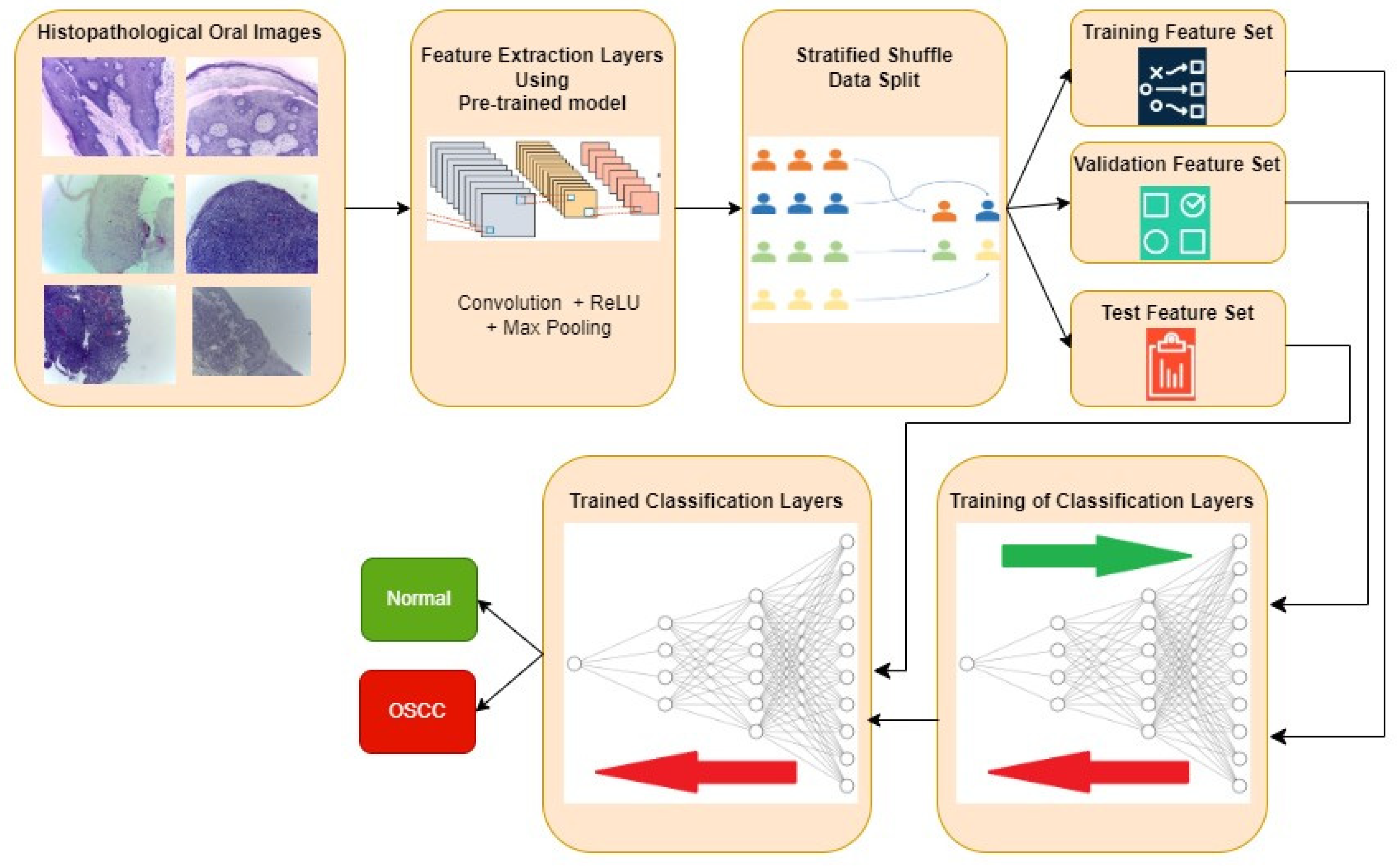
The typical procedure for implementing the oral cancer detection using transfer learning-based feature extraction is shown in
Figure 3. Histopathological oral images from the three datasets are fed to the feature extraction layers discretely and resultant classification performance metrics are also computed individually. Features are extracted using the transfer learning approach where the weights are pre-trained for another similar dataset. Three popular CNN architectures namely InceptionV2, MobileNetV3, and EfficientNetB3 are investigated in this work for feature extraction. Weights that are pre-trained for popular ImageNet dataset is considered in all the three architectures. The extracted features are then divided into training, validation, and test feature sets using stratified shuffle split approach in the 70:15:15 ratio respectively. Stratified shuffle split is considered since it randomly selects the samples according to the class ratio in the original dataset. In other words, stratified shuffle split ensures the ratio of each class in all the three resultant sets as same as shown in
Table 1. This approach of data splitting is very crucial in imbalanced datasets. Then the classification layers are trained using training and validation feature sets where the ideal weights of neural networks for classifying the oral histopathological images are found.
Two fully connected Neural Network layers along with batch normalization and dropout are used as classification layers as shown in
Figure 4. Finally, the trained classification layers with ideal weights are used to classify the test feature set as Normal or OSCC class. In
Figure 4, the functional layer depicts the transfer learning based pre-trained model while the remaining layers are used for classification. The specifications of classification layer considered in this research work is presented in
Table 2. For comparison purposes, the classification layer is unaltered for all the datasets and different feature extraction layers. Specifications related to number of epochs and batch size during training, optimizer, early stopping and reduction of learning rate on plateau are also mentioned in
Table 2. Based on the transfer model used for feature extraction layer, the number of trainable parameters of complete deep learning model will vary as shown in
Table 3. The number of features extracted per input image by the three different feature extraction layers are also shown in
Table 3.
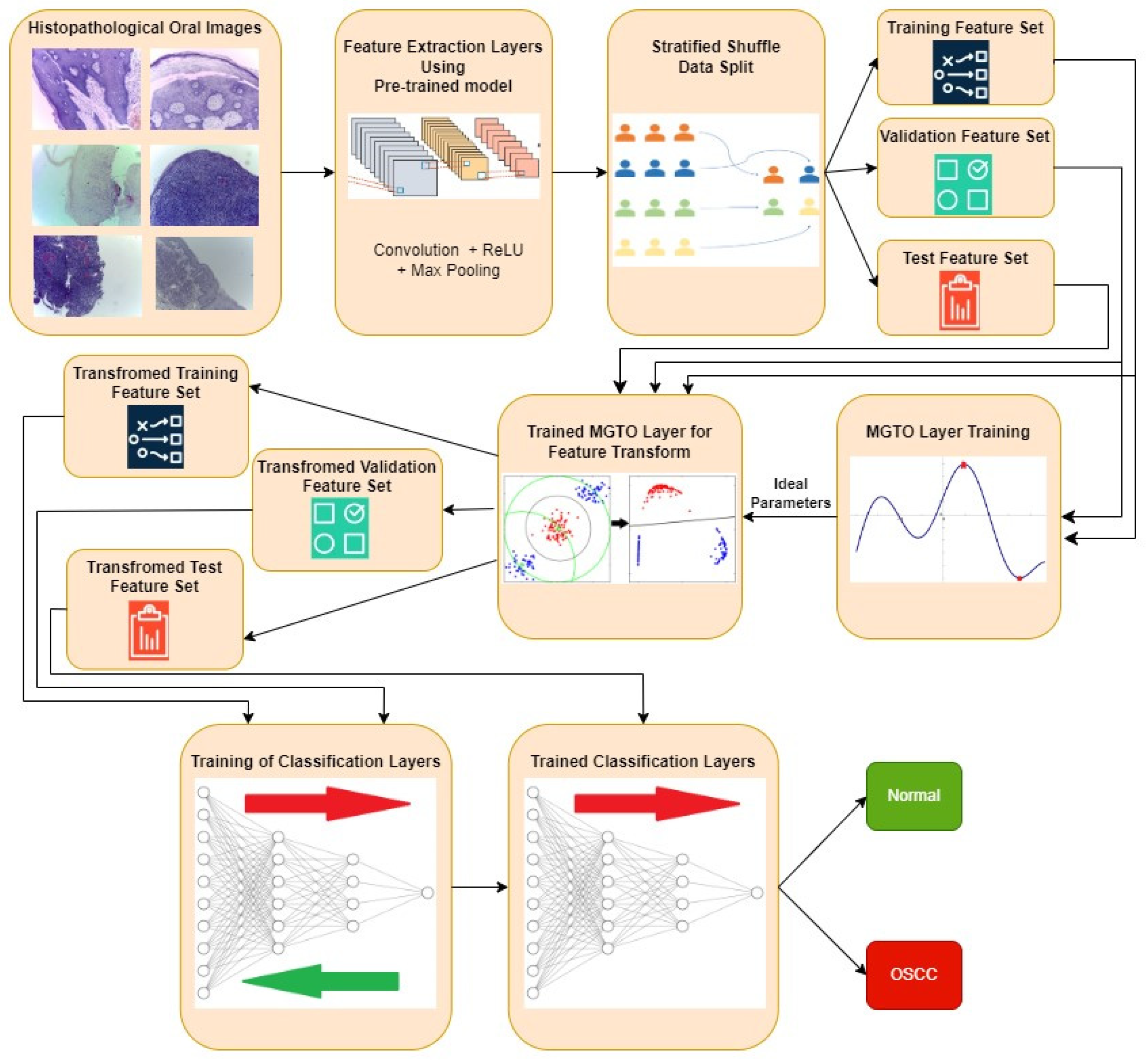
The proposed approach for OSCC detection is presented in
Figure 5 and
Figure 6. An intermediate layer based on MGTO is included in the proposed method when compared to
Figure 3 and
Figure 4. Like classification layer, the newly introduced intermediate layer also needs to be trained where it will learn the ideal values for its parameters related to the MGTO algorithm. Hence it will be trained with original training and validation feature sets. Then all the three original feature sets will be supplied as input to the trained MGTO layer where the features sets are transformed to produce another three transformed sets namely training, testing, and validation. The size of the input and output feature sets remains same. Then the transformed sets are considered for classification layers for detecting the class of oral histopathological image. This research work is carried out in a system with following configurations: i9 processor with 32GB RAM and NVIDIA RTX A2000 12GB GPU.
5. Implementation of Proposed MGTO
The equations to update the Gorilla’s position are modified based on Sine Cosine Algorithm [
48] to increase the exploitation and exploration capabilities of GTO. In MGTO, three equations that update the position of Gorillas are modified. Equations (1), (6), and (9) of GTO are modified as represented in equations (21), (22), and (23) respectively in MGTO. All other equations of GTO remain intact in MGTO.
in the above equations is computed using equation (24).
in equation (24) is a constant and it is considered as three as suggested in [
48];
represents the current iteration number while
represents the maximum number of iterations.
original GTO, the Gorilla’s population is initialized randomly. But to use MGTO as intermediate layer in deep learning models, the Gorilla’s population is initialized with the features extracted from the previous layer. Number of Gorillas will be equal to the number of features extracted. Then the Gorilla’s position will be updated in each iteration using MGTO equations. Fitness function is very crucial in optimization algorithms, and it will be selected based on the problem to be solved. To use MGTO for transforming the features, the fitness function based on variance metric is considered. Fitness of each Gorilla,
will depend on its own position and four nearest-neighbour Gorillas as shown in equation (25).
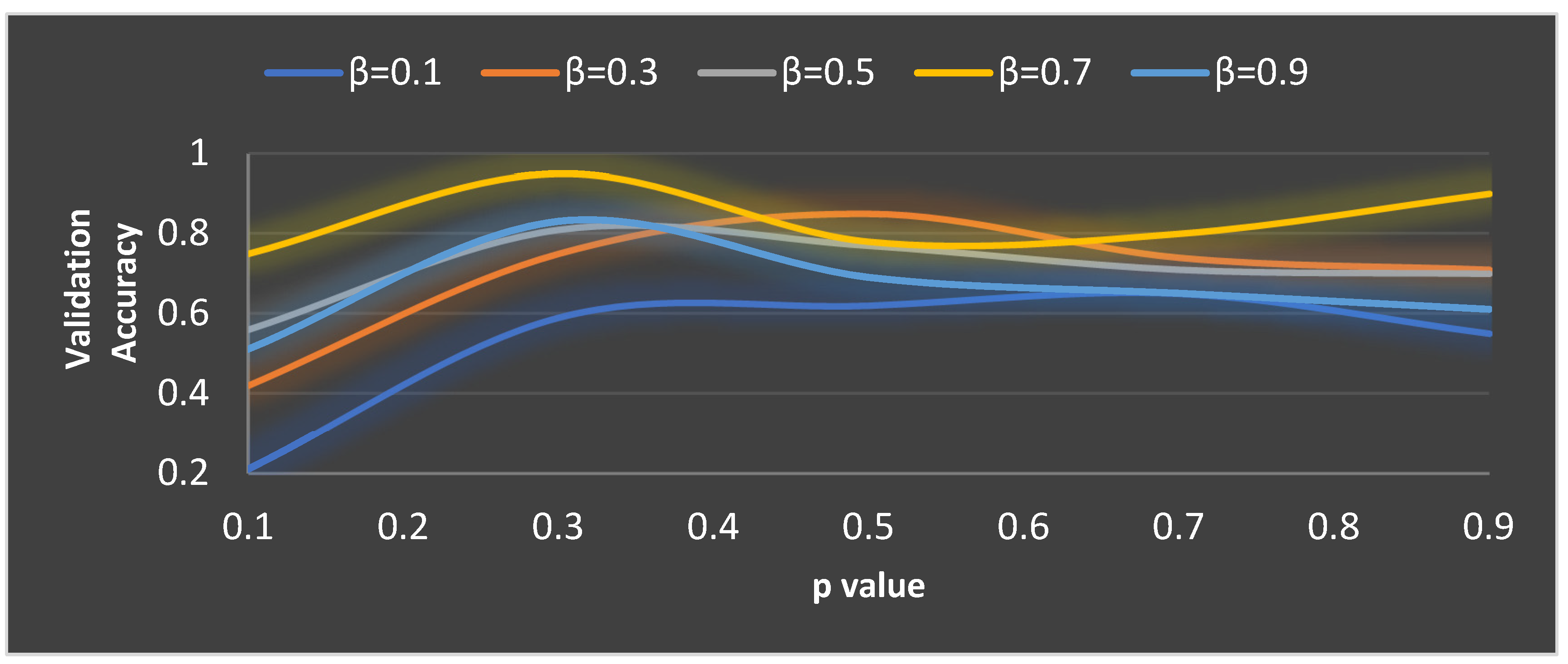
In MGTO,
and
are the parameters which mainly decides the performance along with
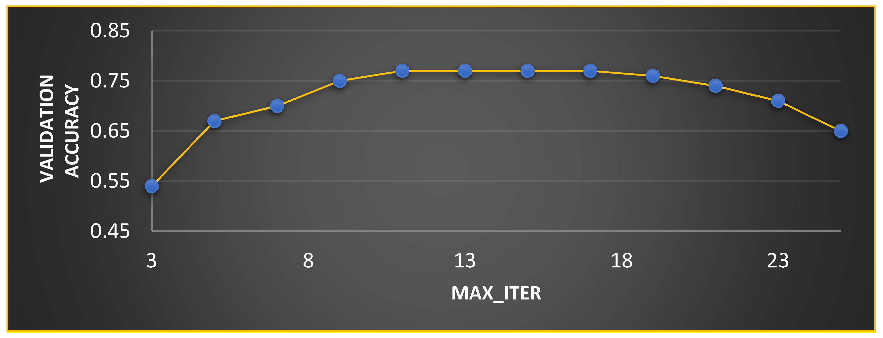
. The ideal values of these parameters are found based on the accuracy attained during training and validation. Validation accuracy for various values of
is plotted in
Figure 7 and
Figure 11 is found as ideal value where the validation accuracy of 0.77 is reached. While finding the optimal value for
, other two parameters namely
and
are kept as 0.5 (median of range [0,1]). To find the optimal values for
and
parameters,
is kept at its ideal value 11.
Figure 8 depicts the validation accuracy for various values of
and
parameters. Highest validation accuracy of 0.95 is attained when
= 0.3 and
= 0.7. Finding the ideal values for the parameters of MGTO is termed as training and for this purpose, training and validation feature sets are used. After training, MGTO transform will be implemented for all the three feature sets namely training, validation, and test sets with the ideal parameters value of
= 0.3, and
= 0.7. Notably these are the ideal parameters of MGTO on first dataset when MobileNetV3 is employed as feature extraction layer. The ideal parametric values may change depending upon the input data given to MGTO layer. The ideal values for other input data will be presented in the next section. Procedure for implementing the MGTO as intermediate feature transform layer for test feature set is summarized in Algorithm 1.
Algorithm 1: Algorithm to implement the proposed MGTO as intermediate layer in deep learning models for feature transformation of test feature set.
-------------------------------------------------------------------------------------------------------------
Step 1: Extract features using pre-trained transfer learning models for each oral histopathological image.
Step 2: Consider number of features as size of population in MGTO. Initialize the position of Gorillas with extracted features.
Step 3: Initialize parameters of MGTO: , , = 0.3, and = 0.7
Step 4: Compute the fitness value of each Gorilla using equation (25)
Step 5: Update the position of each Gorilla using equation (21)
Step 6: Identify the Silverback Gorilla i.e., the Gorilla with highest fitness.
Step 7: Update the position of each Gorilla using equation (22) if . Otherwise use equation (23)
Step 8: Repeat steps 4 to 7 until maximum number of iterations is reached. If the maximum number of iterations are completed, then go to step 9.
Step 9: Consider the final position of Gorillas as the output of Feature Transform and give them as input to the classification layer.
------------------------------------------------------------------------------------------------------------------
and parameters.
6. Results and Discussion
Initially the experiment is conducted without any intermediate layer in the deep learning model. Three different transfer learning-based models namely InceptionV2, MobileNetV3, and EfficientNetB3 are tested as feature extraction layers. As mentioned in
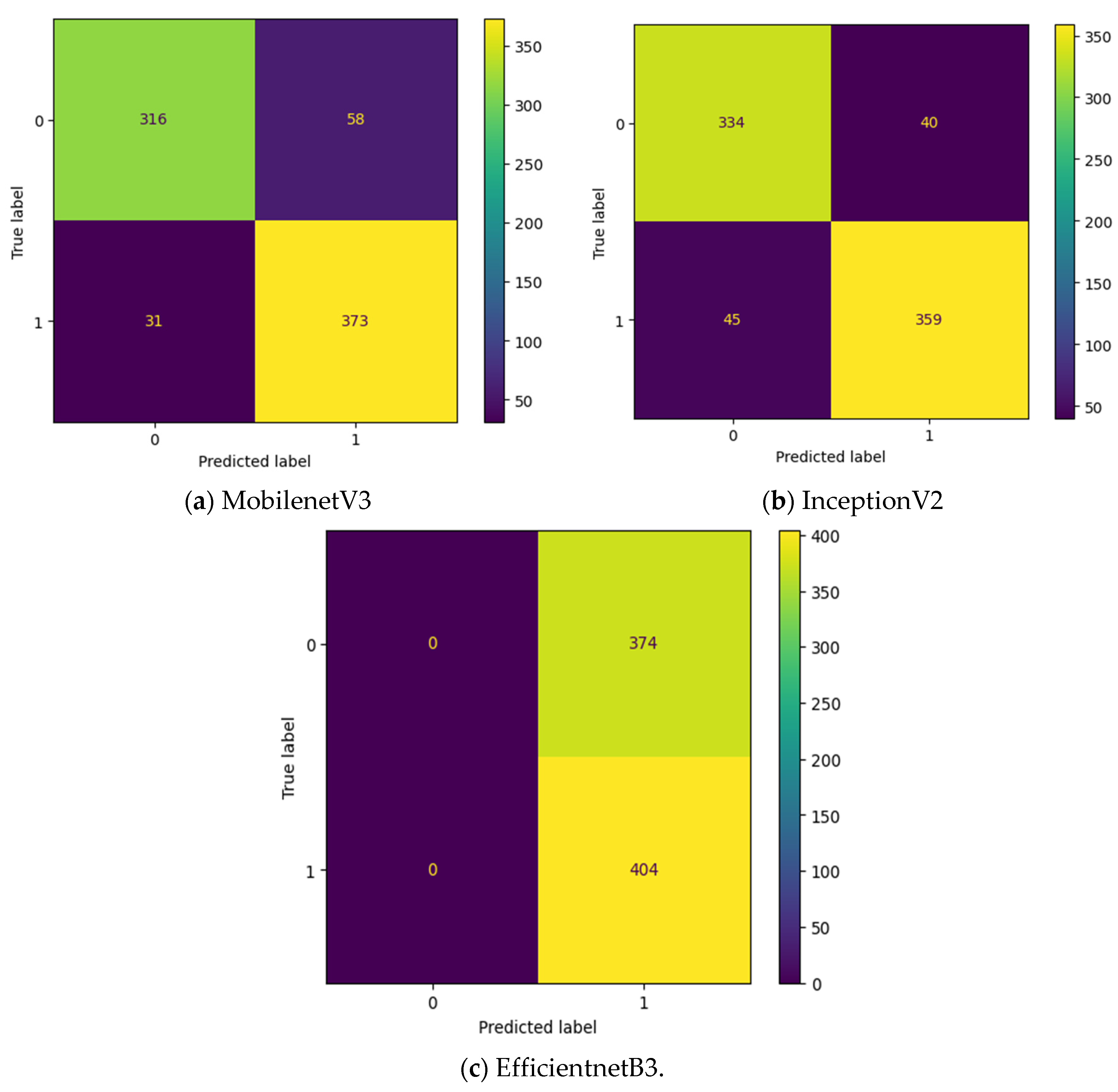
Table 2, the specifications of classification layer remain the same for all the three different feature extraction layers. The confusion matrix attained for these three deep learning models without intermediate layer on first dataset in OSCC detection is shown in
Figure 9. The label 0 represents the class Normal and label 1 represents the class OSCC in
Figure 9. EfficientNetB3 classify all the input images as OSCC and so its True Negative (TN) = 0. This clearly indicates the poor performance of the EfficientNetB3 based deep learning model without intermediate layer. To detect OSCC, high TP is required while to detect normal class properly, high TN is required. Among the remaining two models without intermediate layer, highest True Positive (TP) is attained by MobileNetV3 while the highest TN is attained by InceptionV2.
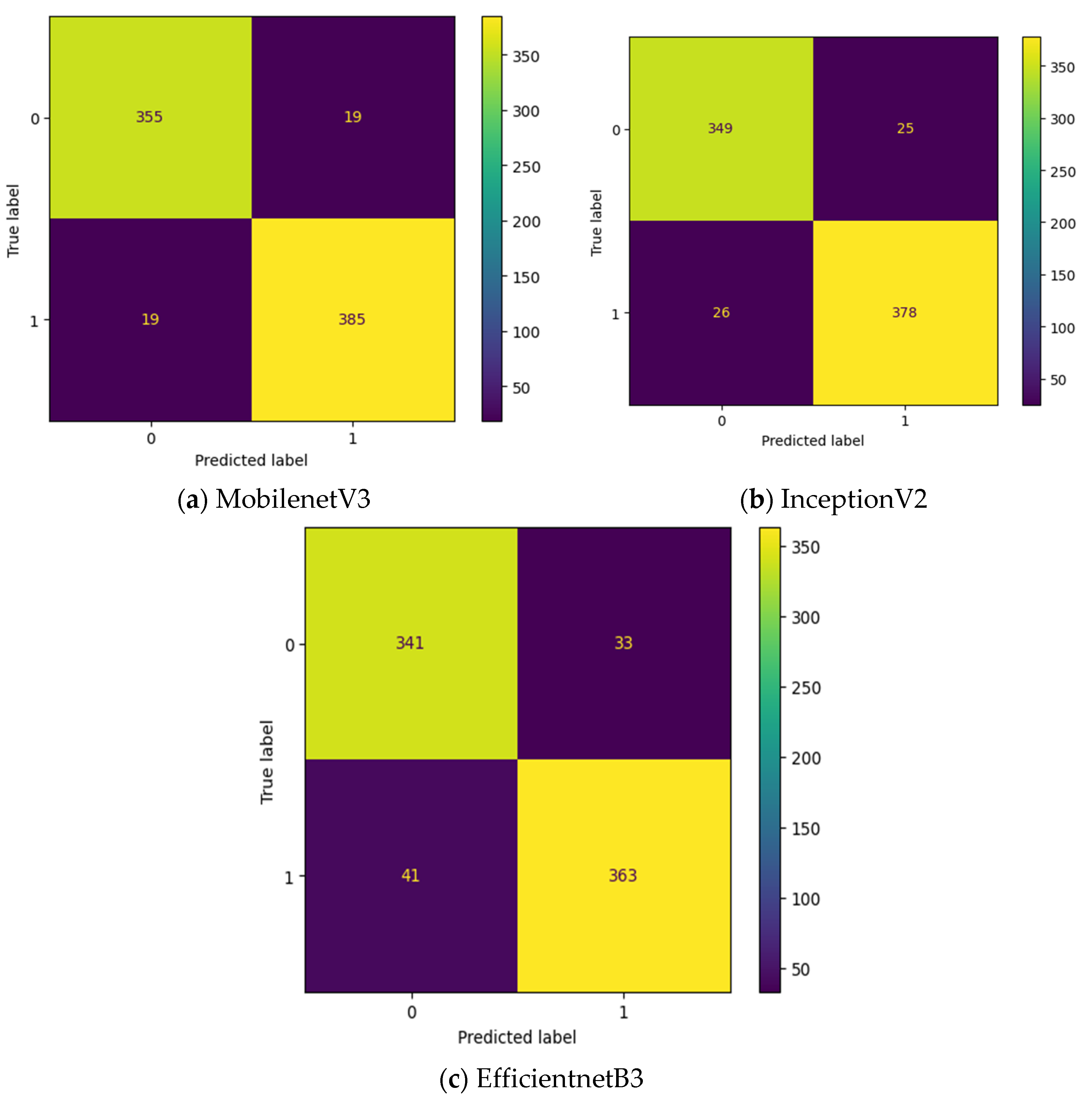
To improve the number of TN and TP, MGTO based intermediate layer is proposed in this work.
Figure 10. shows the confusion matrix of three different feature extraction-based deep learning models with MGTO as intermediate layer in OSCC detection. When MGTO is not used as intermediate layer in EfficientNetB3 based deep learning model, then all the oral images are classified as OSCC while better TN and TP values are attained with the proposed layer. Highest TN and TP values are attained for the proposed MobileNetV3 based feature extraction with MGTO as intermediate layer.
Based on the confusion matrix, four popular performance metrics namely Accuracy, Precision, Recall, and F1-score are used in this research work to analyse the performance of deep learning models. Apart from deep learning models with and without MGTO based intermediate layer, three other swarm intelligence-based optimization algorithms namely PSO, EHO, and GTO are also tested as intermediate layer and their results are also presented in
Table 4. Implementation procedure for PSO, EHO, and GTO as intermediate layer will also follow the Algorithm 1 presented in previous section. Only the parameters and the way of updating the position of Swarm will vary based on the optimization algorithm used. The final ideal parameters of all the four tested intermediate layer after training is listed in
Table 5.
The main objective of this work is to detect OSCC and so precision, recall, and F1-score in
Table 4 are related to truthful identification of OSCC class while the accuracy metric is related to truthful identification of both normal and OSCC classes. As seen in
Table 4, deep learning models without any intermediate layer provides less accuracy than the proposed deep learning models with MGTO as intermediate layer.
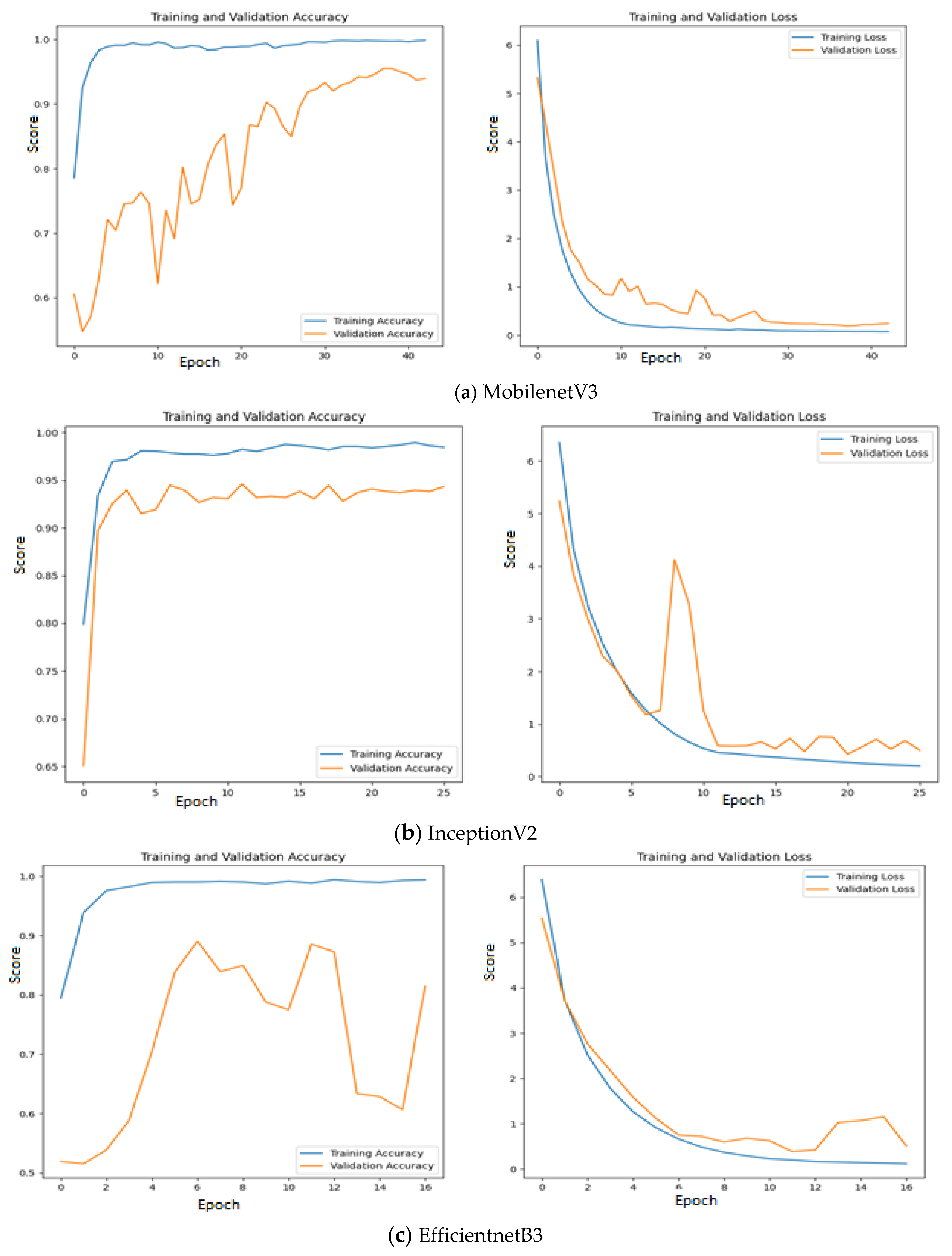
Figure 11.
Training & validation accuracy and loss of Deep learning models without intermediate layer on first dataset.
Figure 11.
Training & validation accuracy and loss of Deep learning models without intermediate layer on first dataset.
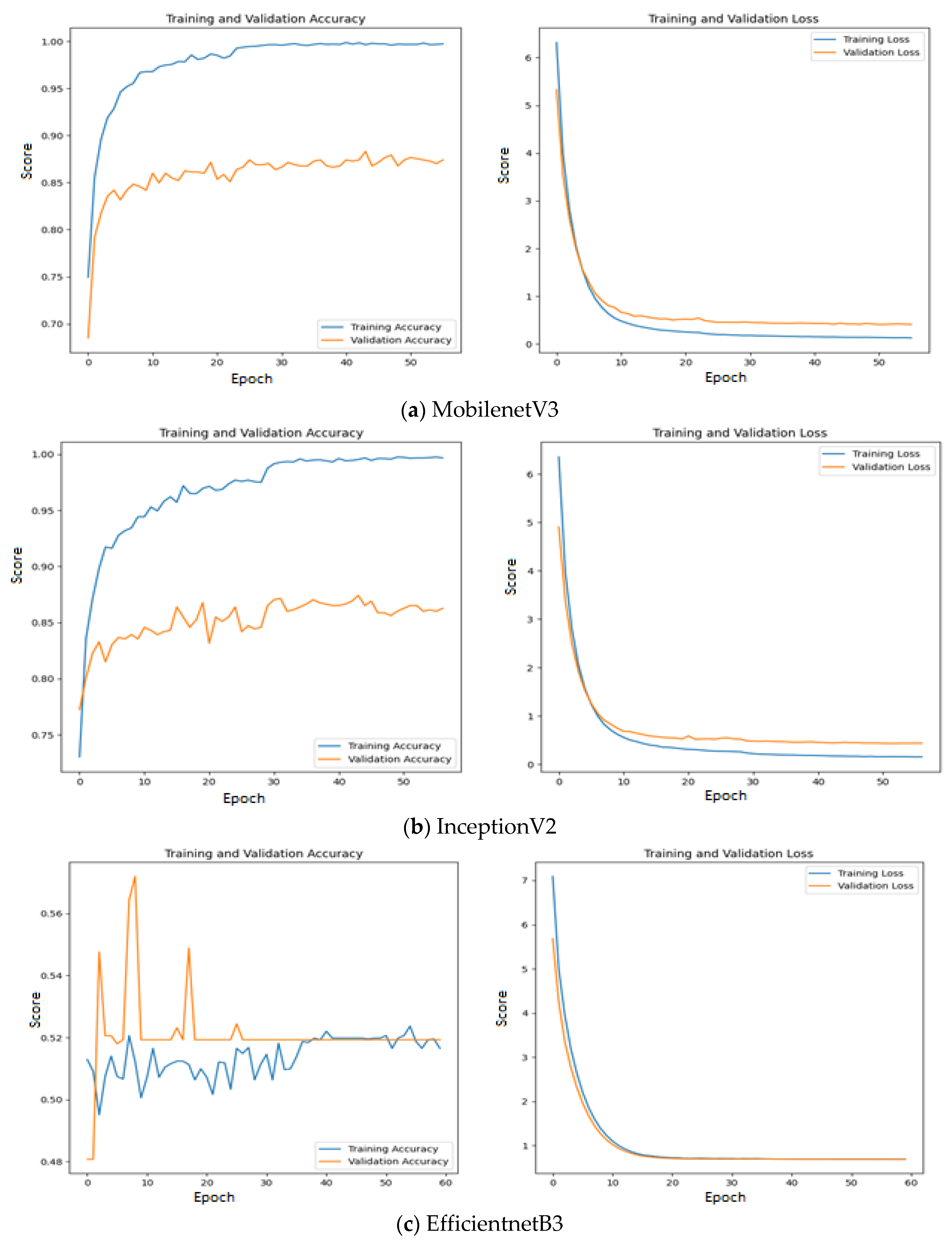
Among the models without intermediate layer, MobileNetV3 offers highest accuracy of 0.89 which is followed by InceptionV2 with accuracy of 0.88 and EfficientNetB3 with accuracy of 0.52. The reason for such poor performance of EfficientNetB3 is explained as follows: All the three feature extraction models are pre-trained on ImageNet dataset and features are extracted based on the weights appropriate for ImageNet dataset. The weights and architecture of EfficientNetB3 fails to capture the significant features from input oral images while vital features are properly extracted by the remaining two feature extraction models. This statement is further supported by
Figure 11 where the training and validation accuracy & loss are presented for all the three investigated deep learning models without intermediate layer on the first dataset.
Since quality features are extracted by MobileNetV3 and InceptionV2, both training & validation accuracy are increasing gradually during training. In addition, both training & validation loss are also decreasing in exponential manner. But deep learning model that uses EfficientNetB3 fails to grow both training and validation accuracy due to poor features extracted from the histopathological oral images.
Figure 12 presents the training & validation accuracy and loss when MGTO is used as intermediate layer on the first dataset. It clearly shows the improved accuracy during both training and validation because of transformed appropriate features produced by MGTO. To support the findings based on first dataset, other two smaller OSCC datasets are tested. The second and third dataset are highly imbalanced since the number of OSCC class samples is much higher than the number of normal class samples. The performance metrics attained on those two datasets are presented in
Table 6 and
Table 7.
From the
Table 4,
Table 6, and
Table 7, it is very clear that MGTO works very well as intermediate layer when compared to other tested intermediate layers in all the three datasets. The significance of MGTO as intermediate layer can be clearly witnessed in
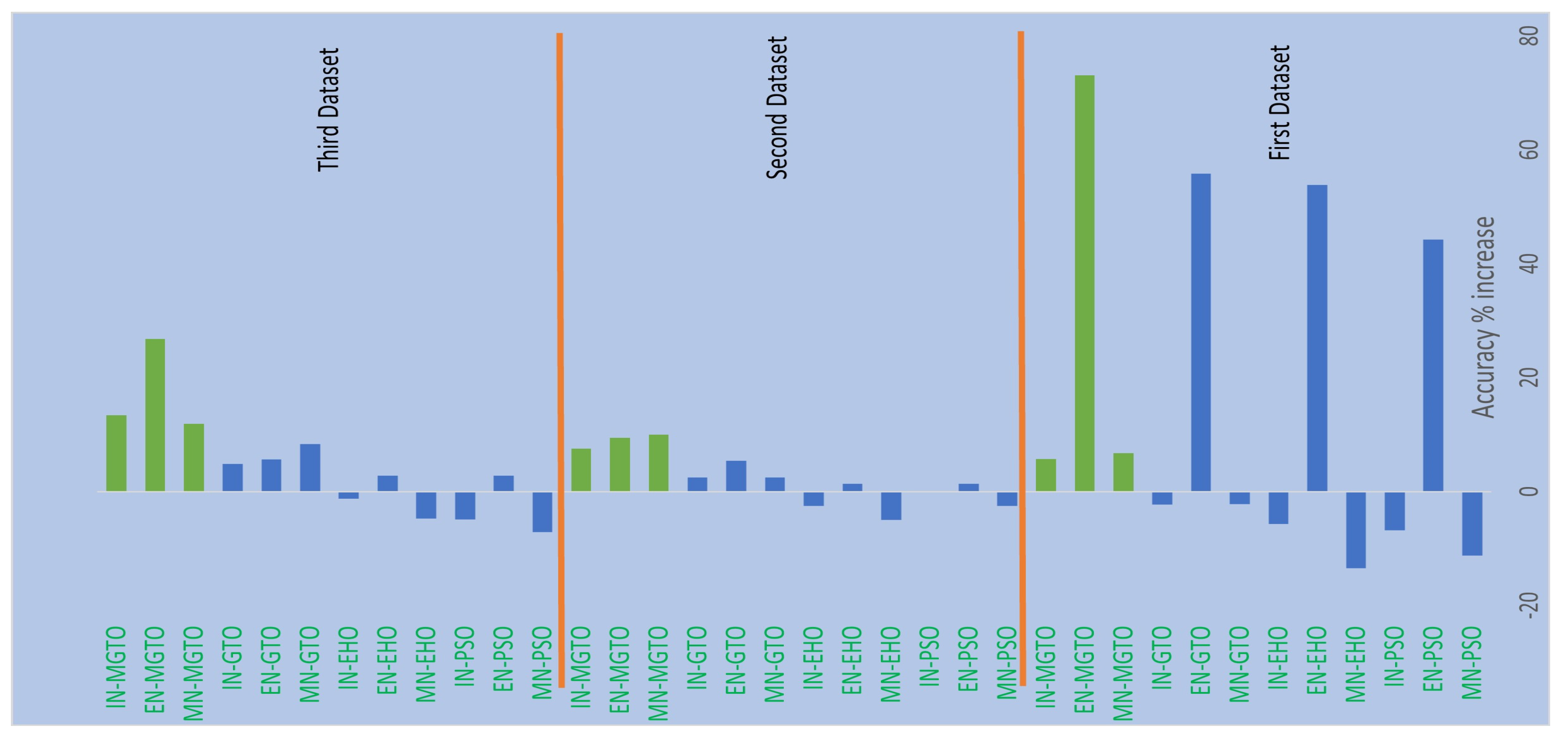
Figure 13 where percentage of accuracy increase attained by the usage of various intermediate layers when compared to deep learning model without intermediate layer is depicted.
On all the three datasets, the percentage of accuracy increase is very less or even negative when PSO, EHO, & GTO are used as intermediate layer on the features extracted from MobileNetV3 and InceptionNetV2. Notably, already these two feature extraction models without intermediate layer produces accuracy of more than 0.8 in all the three datasets. Implicitly, these intermediate layers fails to significantly improve the accuracy since they are not able to produce more appropriate transformed features for classification. Only on the features extracted by EfficientNetB3 of first dataset, these intermediate layers are able to provide significant accuracy increase since the original features extracted by EfficientNetB3 is very poor on the first dataset which yield accuracy of only 0.52. Out of these three intermediate layers, GTO comparatively performs well on all the three datasets. Hence intuition for improving GTO further with suitable modifications raised. MGTO is formulated with the modifications stated in the previous section and it worked well on all the three datasets.
In the first dataset, 73% of increase in accuracy is witnessed on the EfficientNetB3 based DL model due to the usage of MGTO as intermediate layer. Nearly 6% accuracy is increased due to MGTO on MobileNetV3 and InceptionV2 based DL models. Notably the highest accuracy 0.95 is produced on the first dataset by MobileNetV3-MGTO based DL model. Even on the imbalanced second and third datasets, MGTO is capable of producing significant accuracy increase. The reason for this better performance is threefold. Firstly, the modification of GTO with Sine and Cosine algorithm increases its exploration and exploitation capability well. Exploitation is responsible for local search i.e., fine-tuning and exploration is responsible for global search. Secondly, the selection of appropriate fitness function. Local variance based fitness function worked well to transform the features of different classes in different way. Thirdly, the usage of ideal parameters in MGTO resulted in better accuracy. As shown in
Figure 7 &
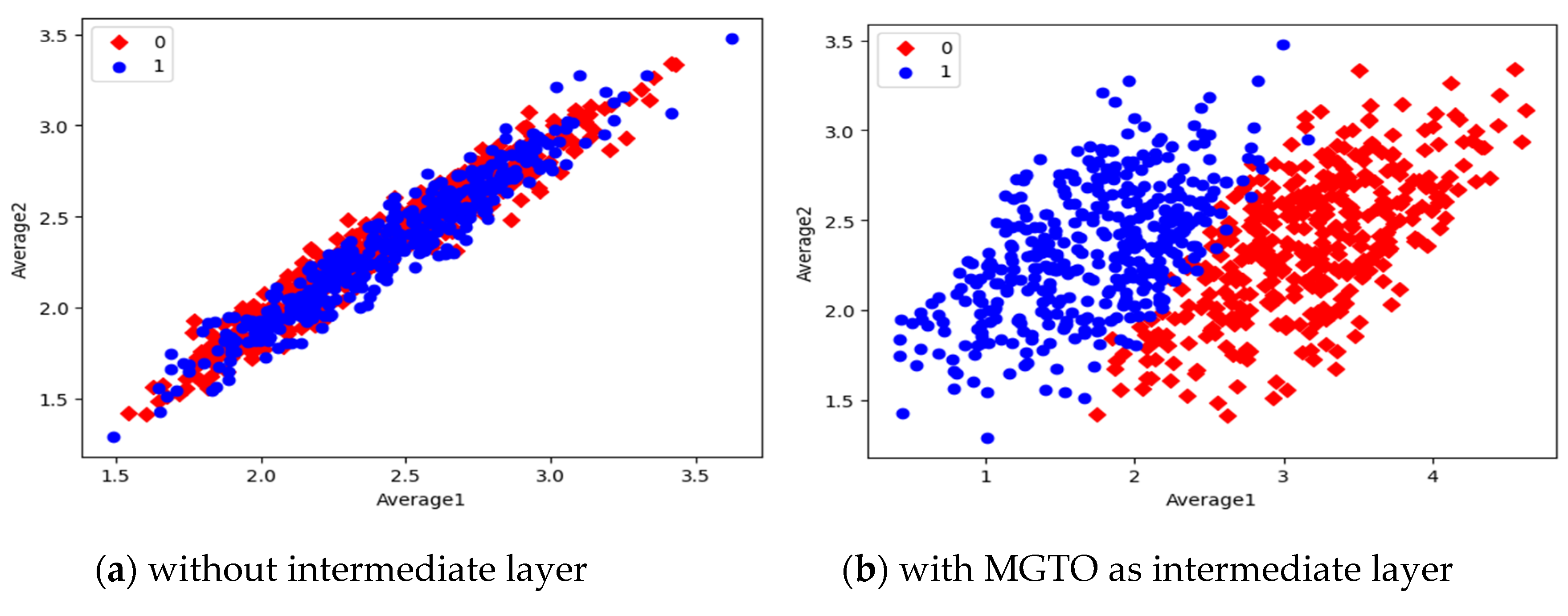
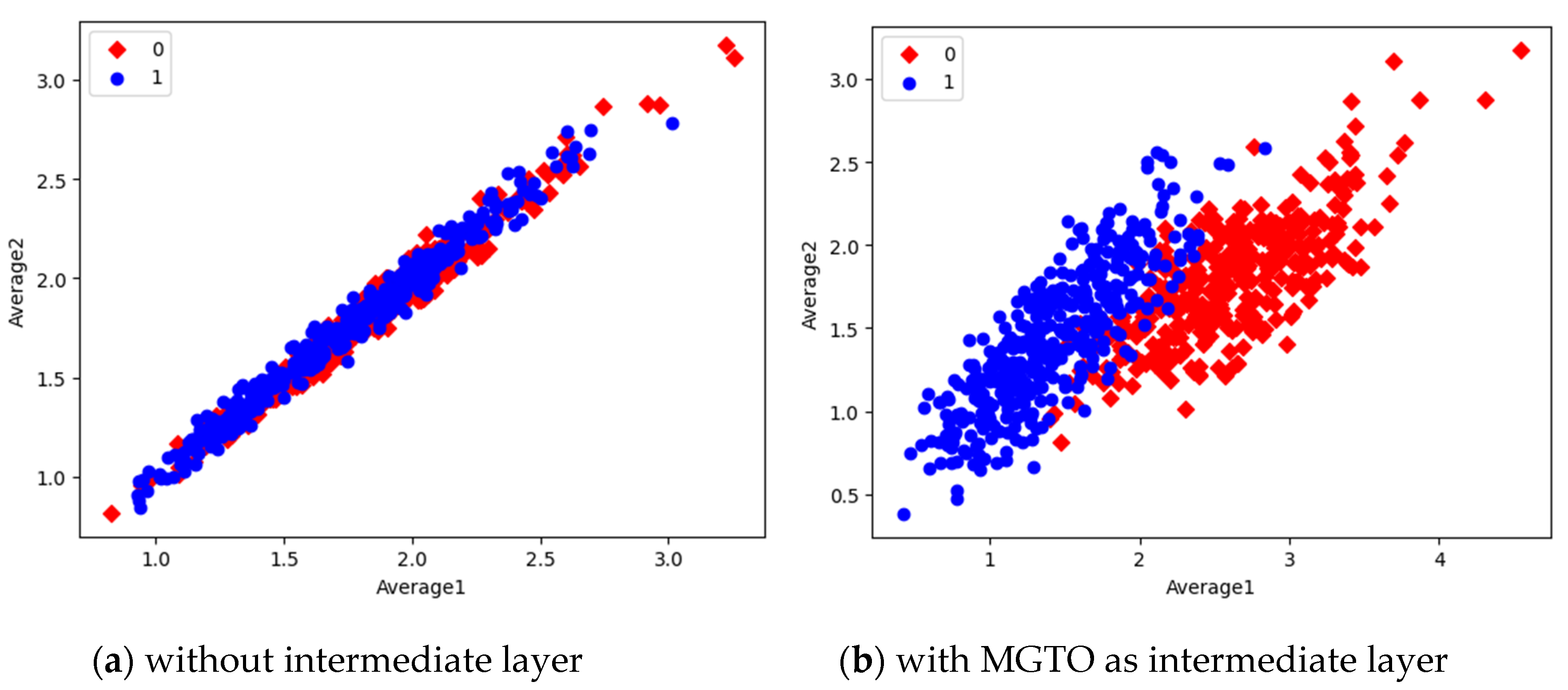
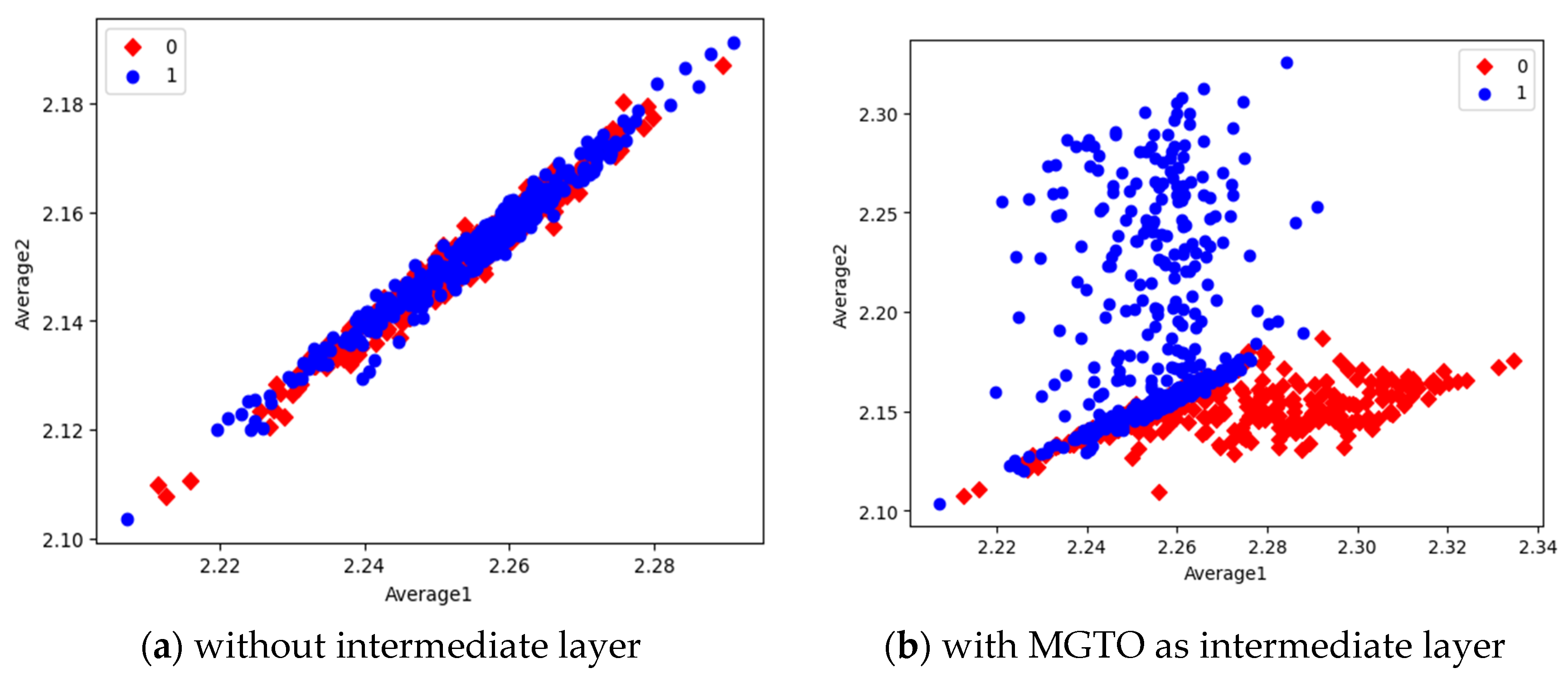
Figure 8, values of MGTO parameters will have huge impact on accuracy. Due to the above mentioned reasons, MGTO works soundly as intermediate layer that transforms the input features into more-appropriate features for classification. In other words, the introduction of proposed intermediate layer helps the classifier to distinguish the features of two different classes. This statement is backed by the scatter plots shown in
Figure 14,
Figure 15, and
Figure 16. In scatter plots, the label 0 represents the class Normal and label 1 represents the class OSCC. To represent the features of first dataset in scatter plot, two averages are computed. Average1 is the mean of first half features and Average2 is the mean of remaining half features. For example, 1280 features are extracted by MobileNetV3; mean of first 640 features are considered as Average1 and remaining 640 features are considered as Average2.
Comparison of three scatter plots without intermediate layer, gives the reasons for better performance of MobileNetV3 and poor performance of EfficientNetB3. MobileNetV3 features of two classes are slightly scatter and overlapped while EfficientNetB3 features are heavily overlapped. On comparison of scatter plots with and without intermediate layers of all the three feature extraction models, clearly suggests the significance of MGTO. The proposed layer transforms the features in a manner that is more suitable for classification by spreading the two different class features apart to some extent. When these transformed features are used for training and validation, then the classification layer gets trained well. Finally better performance is achieved when transformed test dataset is categorized by the trained classification layer.
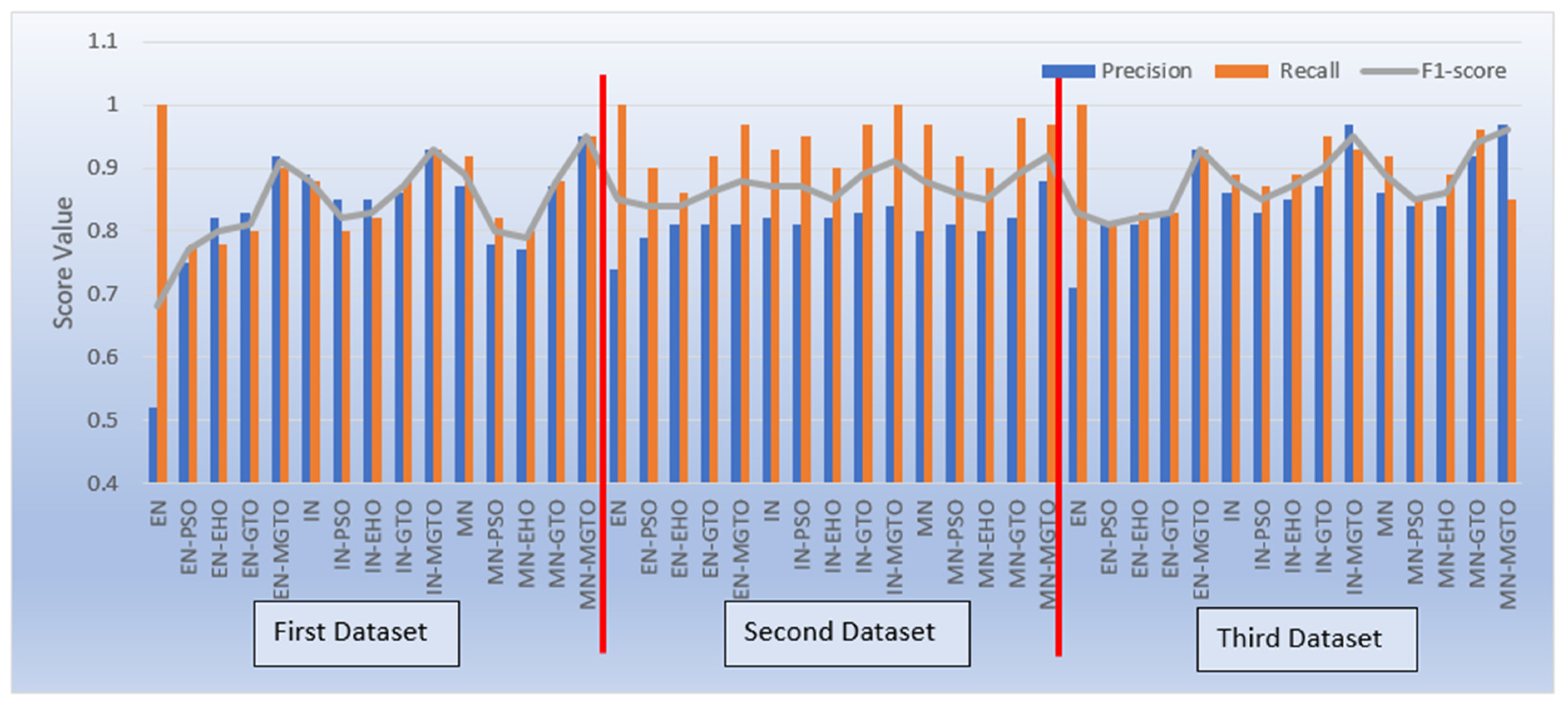
Apart from accuracy, other performance metrics are also relevantly important. Precision gives the percentage of correct OSCC predictions among total number of OSCC predicted. Recall is related to percentage of actual OSCC which was identified correctly as OSCC. F1 score is the harmonic mean of precision and recall score. These metrics are depicted for all the three datasets in
Figure 17. Considering these three metrics, DL models with MGTO as intermediate layer outperforms all other investigated intermediate layers. In the first dataset, highest performance is offered by the proposed MobileNetV3-MGTO based DL model through which precision = 0.95, recall = 0.95, and F1-score = 0.95 is achieved. Even on the second and third datasets, highest F1 score is archived by the proposed DL model. Though highest F1 score and accuracy is attained by the proposed DL model on all the three datasets, it fails to attain balanced precision and recall in imbalanced datasets. For example, recall is very much higher than precision for the proposed DL model in second dataset while precision is very much higher than recall for the proposed DL model in third dataset. But it attains almost equal precision and recall in first dataset which is a balanced dataset. Hence wherever higher values of both precision and recall is required on imbalanced dataset, the proposed DL model underperforms there. This could be considered as first limitation of proposed model.
Training time of all the investigated DL models on the first dataset is presented in
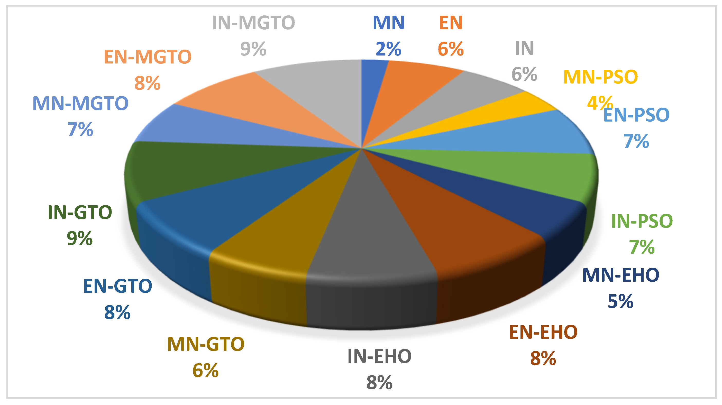
Table 8. DL models without intermediate layer will get trained comparatively quickly while the presence of intermediate layer may take more training time. MobileNetV3 have less training time since the number of features extracted is 1280 while the number of features extracted by EfficientNetB3 and InceptionNetV2 is 1536. A pie chart is presented in
Figure 18 which depicts the percentage of time taken by a DL model when compared to the total training time taken by all the DL models. PSO and EHO takes relatively less training time than other intermediate layers due to their simple structure. When compared to GTO, the proposed MGTO intermediate layer will take more training time due to the inclusion of sine and cosine argument calculations. Only 2% of total training time is taken by MobileNetV3 DL model without any intermediate layer while 7% of total training time is taken by the proposed DL model. This could be considered as second limitation.
The accuracy comparison of some related works for oral cancer detection is presented in
Table 9. Supervised classifiers such as K-Nearest Neighbour, Support Vector machine attains comparatively lesser accuracy than the deep learning models. The proposed deep learning model with MGTO as intermediate layer offers the highest accuracy of 95% and shows the importance of proposed DL model.
Figure 1.
Sample oral histopathological images belonging to Normal class.
Figure 1.
Sample oral histopathological images belonging to Normal class.
Figure 2.
Sample oral histopathological images belonging to OSCC class.
Figure 2.
Sample oral histopathological images belonging to OSCC class.
Figure 3.
Typical approach for OSCC detection using Transfer learning-based feature extraction.
Figure 3.
Typical approach for OSCC detection using Transfer learning-based feature extraction.
Figure 4.
Typical deep learning architecture with functional layer depicting the transfer learning model for feature extraction and remaining layers depicting the classification layers.
Figure 4.
Typical deep learning architecture with functional layer depicting the transfer learning model for feature extraction and remaining layers depicting the classification layers.
Figure 5.
Overview of Proposed Approach for OSCC Detection.
Figure 5.
Overview of Proposed Approach for OSCC Detection.
Figure 6.
Proposed deep learning architecture where MGTO is used as intermediate layer between feature extraction (functional) layer and classification layer. .
Figure 6.
Proposed deep learning architecture where MGTO is used as intermediate layer between feature extraction (functional) layer and classification layer. .
Figure 7.
Ideal value computation for
Figure 7.
Ideal value computation for
Figure 8.
Ideal value computation of
Figure 8.
Ideal value computation of
Figure 9.
Confusion Matrix of Deep learning models without intermediate layer.
Figure 9.
Confusion Matrix of Deep learning models without intermediate layer.
Figure 10.
Confusion Matrix of Deep learning models with MGTO as intermediate layer.
Figure 10.
Confusion Matrix of Deep learning models with MGTO as intermediate layer.
Figure 12.
Training & validation accuracy and loss of Deep learning models with MGTO as intermediate layer on first dataset.
Figure 12.
Training & validation accuracy and loss of Deep learning models with MGTO as intermediate layer on first dataset.
Figure 13.
Percentage accuracy increase due to the usage of intermediate layers in DL models when compared to the accuracy offered by DL models without intermediate layer.
Figure 13.
Percentage accuracy increase due to the usage of intermediate layers in DL models when compared to the accuracy offered by DL models without intermediate layer.
Figure 14.
Scatter Plot of features extracted by MobileNetV3.
Figure 14.
Scatter Plot of features extracted by MobileNetV3.
Figure 15.
Scatter Plot of features extracted by InceptioNetV2.
Figure 15.
Scatter Plot of features extracted by InceptioNetV2.
Figure 16.
Scatter Plot of features extracted by EfficientNetB3.
Figure 16.
Scatter Plot of features extracted by EfficientNetB3.
Figure 17.
Precision, Recall, and F1 score of various OSCC classification models.
Figure 17.
Precision, Recall, and F1 score of various OSCC classification models.
Figure 18.
Pie-chart representing the percentage of training time taken by each DL model with respect to total training time taken by all DL models.
Figure 18.
Pie-chart representing the percentage of training time taken by each DL model with respect to total training time taken by all DL models.
Table 1.
Stratified shuffle data split on three datasets.
Table 1.
Stratified shuffle data split on three datasets.
| Dataset |
Class |
Total number of samples |
Number of training samples |
Number of validation samples |
Number of test samples |
| First |
Normal |
2494 |
1746 |
374 |
374 |
| OSCC |
2698 |
1890 |
404 |
404 |
| Second |
Normal |
89 |
63 |
13 |
13 |
| OSCC |
439 |
307 |
66 |
66 |
| Third |
Normal |
201 |
141 |
30 |
30 |
| OSCC |
495 |
347 |
74 |
74 |
Table 2.
Specifications of classification layer and techniques used.
Table 2.
Specifications of classification layer and techniques used.
| Classification layers & techniques used |
Specifications |
| Batch Normalization |
momentum= 0.99, epsilon= 0.001 |
| Dense |
units = 256, kernel regularizer = L2 regularizer with coefficient l = 0.016, activity regularizer = L1 regularizer with coefficient l = 0.006, bias regularizer = L1 regularizer with coefficient l = 0.006, activation= ReLu |
| Dropout |
drop rate= 0.45 |
| Dense |
units = 2, activation= SoftMax |
| Training |
epochs = 100, batch size = 128, stratified shuffle split: training - 70%, testing - 15%, validation -15% |
| Optimizer |
Adamax with learning rate= 0.001, loss= sparse categorical cross-entropy, metrics=accuracy |
| Early stopping |
patience = 5, minimum delta = 0, monitor = validation loss, restore best weights = True, mode = minimum |
| Reduce learning rate on Plateau |
monitor = validation loss, factor = 0.2, patience = 4, mode = minimum |
Table 3.
Specifications of Feature extraction layer.
Table 3.
Specifications of Feature extraction layer.
| Feature extraction Layers |
Total number of parameters |
Number of Trainable parameters |
Number of features extracted |
| Mobilenet V3 |
25,91,554 |
3,31,010 |
1280 |
| Efficientnet B3 |
1,11,83,665 |
3,97,058 |
1536 |
| InceptionV2 |
5,47,36,866 |
3,97,058 |
1536 |
Table 4.
Performance metrics computed on test set of first dataset.
Table 4.
Performance metrics computed on test set of first dataset.
| Transfer learning model |
Intermediate layer |
Accuracy |
Precision |
Recall |
F1-score |
| MobilenetV3 |
NO |
0.89 |
0.87 |
0.92 |
0.89 |
| EfficientnetB3 |
NO |
0.52 |
0.52 |
1 |
0.68 |
| InceptionV2 |
NO |
0.88 |
0.89 |
0.88 |
0.88 |
| MobilenetV3 |
PSO |
0.79 |
0.78 |
0.82 |
0.8 |
| EfficientnetB3 |
PSO |
0.75 |
0.75 |
0.78 |
0.77 |
| InceptionV2 |
PSO |
0.82 |
0.85 |
0.8 |
0.82 |
| MobilenetV3 |
EHO |
0.77 |
0.77 |
0.8 |
0.79 |
| EfficientnetB3 |
EHO |
0.8 |
0.82 |
0.78 |
0.8 |
| InceptionV2 |
EHO |
0.83 |
0.85 |
0.82 |
0.83 |
| MobilenetV3 |
GTO |
0.87 |
0.87 |
0.88 |
0.88 |
| EfficientnetB3 |
GTO |
0.81 |
0.83 |
0.8 |
0.81 |
| InceptionV2 |
GTO |
0.86 |
0.86 |
0.88 |
0.87 |
| MobilenetV3 |
MGTO |
0.95 |
0.95 |
0.95 |
0.95 |
| EfficientnetB3 |
MGTO |
0.9 |
0.92 |
0.9 |
0.91 |
| InceptionV2 |
MGTO |
0.93 |
0.93 |
0.93 |
0.93 |
Table 5.
Ideal parameters of various intermediate layers.
Table 5.
Ideal parameters of various intermediate layers.
| Feature extraction |
Intermediate layer |
Ideal Parameter values |
| MobilenetV3 |
PSO |
Max_Iter = 10, w=0.6, c1=0.7, and c2=0.9 |
| EHO |
Max_Iter = 12, = 0.9, and =0.8 |
| GTO |
= 0.2, and = 0.7 |
| MGTO |
= 0.3, and = 0.7 |
| EfficientnetB3 |
PSO |
Max_Iter = 12, w=0.4, c1=0.7, and c2=0.9 |
| EHO |
Max_Iter = 12, = 0.7, and =0.8 |
| GTO |
= 0.5, and = 0.7 |
| MGTO |
= 0.3, and = 0.8 |
| InceptionV2 |
PSO |
Max_Iter = 12, w=0.6, c1=0.8, and c2=0.8 |
| EHO |
Max_Iter = 11, = 0.8, and =0.6 |
| GTO |
= 0.4, and = 0.7 |
| MGTO |
= 0.4, and = 0.6 |
Table 6.
Performance metrics computed on test set of second dataset.
Table 6.
Performance metrics computed on test set of second dataset.
| Transfer learning model |
Intermediate layer |
Accuracy |
Precision |
Recall |
F1-score |
| MobilenetV3 |
NO |
0.8 |
0.8 |
0.97 |
0.88 |
| EfficientnetB3 |
NO |
0.74 |
0.74 |
1 |
0.85 |
| InceptionV2 |
NO |
0.8 |
0.82 |
0.93 |
0.87 |
| MobilenetV3 |
PSO |
0.78 |
0.81 |
0.92 |
0.86 |
| EfficientnetB3 |
PSO |
0.75 |
0.79 |
0.9 |
0.84 |
| InceptionV2 |
PSO |
0.8 |
0.81 |
0.95 |
0.87 |
| MobilenetV3 |
EHO |
0.76 |
0.8 |
0.9 |
0.85 |
| EfficientnetB3 |
EHO |
0.75 |
0.81 |
0.86 |
0.84 |
| InceptionV2 |
EHO |
0.78 |
0.82 |
0.9 |
0.85 |
| MobilenetV3 |
GTO |
0.82 |
0.82 |
0.98 |
0.89 |
| EfficientnetB3 |
GTO |
0.78 |
0.81 |
0.92 |
0.86 |
| InceptionV2 |
GTO |
0.82 |
0.83 |
0.97 |
0.89 |
| MobilenetV3 |
MGTO |
0.88 |
0.88 |
0.97 |
0.92 |
| EfficientnetB3 |
MGTO |
0.81 |
0.81 |
0.97 |
0.88 |
| InceptionV2 |
MGTO |
0.86 |
0.84 |
1 |
0.91 |
Table 7.
Performance metrics computed on test set of third dataset.
Table 7.
Performance metrics computed on test set of third dataset.
| Transfer learning model |
Intermediate layer |
Accuracy |
Precision |
Recall |
F1-score |
| MobilenetV3 |
NO |
0.84 |
0.86 |
0.92 |
0.89 |
| EfficientnetB3 |
NO |
0.71 |
0.71 |
1 |
0.83 |
| InceptionV2 |
NO |
0.82 |
0.86 |
0.89 |
0.88 |
| MobilenetV3 |
PSO |
0.78 |
0.84 |
0.85 |
0.85 |
| EfficientnetB3 |
PSO |
0.73 |
0.81 |
0.81 |
0.81 |
| InceptionV2 |
PSO |
0.78 |
0.83 |
0.87 |
0.85 |
| MobilenetV3 |
EHO |
0.8 |
0.84 |
0.89 |
0.86 |
| EfficientnetB3 |
EHO |
0.73 |
0.81 |
0.83 |
0.82 |
| InceptionV2 |
EHO |
0.81 |
0.85 |
0.89 |
0.87 |
| MobilenetV3 |
GTO |
0.91 |
0.92 |
0.96 |
0.94 |
| EfficientnetB3 |
GTO |
0.75 |
0.83 |
0.83 |
0.83 |
| InceptionV2 |
GTO |
0.86 |
0.87 |
0.95 |
0.9 |
| MobilenetV3 |
MGTO |
0.94 |
0.97 |
0.85 |
0.96 |
| EfficientnetB3 |
MGTO |
0.9 |
0.93 |
0.93 |
0.93 |
| InceptionV2 |
MGTO |
0.93 |
0.97 |
0.93 |
0.95 |
Table 8.
Time taken for training various DL models.
Table 8.
Time taken for training various DL models.
| DL Model |
Training Time
(hh:mm:ss)
|
DL Model |
Training Time (hh:mm:ss) |
| MN |
00:05:33 |
IN-EHO |
00:18:22 |
| EN |
00:15:42 |
MN-GTO |
00:15:15 |
| IN |
00:14:37 |
EN-GTO |
00:19:17 |
| MN-PSO |
00:09:23 |
IN-GTO |
00:21:39 |
| EN-PSO |
00:17:52 |
MN-MGTO |
00:15:52 |
| IN-PSO |
00:17:01 |
EN-MGTO |
00:20:12 |
| MN-EHO |
00:12:47 |
IN-MGTO |
00:22:21 |
| EN-EHO |
00:18:46 |
|
|
Table 9.
Comparison of accuracy attained in related works.
Table 9.
Comparison of accuracy attained in related works.
| Related Works |
Year |
Classification Framework |
Accuracy (%) attained |
| A. U. Rahman et al. [25] |
2022 |
AlexNet |
90.06% |
| M. Aberville [48] |
2017 |
Convolutional Neural Network |
88.3% |
| H. Alkhadar [49] |
2021 |
KNN, Logistic Regression, Decision Tree, Random Forest |
76% |
| A.Alhazmi [50] |
2021 |
Artificial Neural Network |
78.95% |
| C.S. Chu [51] |
2020 |
SVM, KNN |
70.59% |
| R.A.Welikala [52] |
2020 |
ResNet101 |
78.30% |
| Shavlokhova, V [53] |
2021 |
CNN |
77.89% |
| Proposed |
2023 |
Pre-trained MobileNetV3 for feature extraction and MGTO as intermediate layer |
95% |
