Online Machine Learning and Surrogate Model-Based Optimization for Improved Production Processes Using a Cognitive Architecture

Preprint

Article

Online Machine Learning and Surrogate Model-Based Optimization for Improved Production Processes Using a Cognitive Architecture

Altmetrics

Downloads

Views

Comments

A peer-reviewed article of this preprint also exists.

Submitted:

04 October 2023

Posted:

07 October 2023

You are already at the latest version

Alerts

Abstract

Cyber-Physical Systems (CPS) play an essential role in today’s production processes, leveraging Artificial Intelligence (AI) to enhance operations such as optimization, anomaly detection, and predictive maintenance. This article reviews a cognitive architecture for artificial intelligence, which has been developed to establish a standard framework for integrating AI solutions into existing production processes. Given that machines in these processes continuously generate large streams of data, Online Machine Learning (OML) was identified as a crucial extension to the existing architecture. To substantiate this claim, real-world experiments using a slitting machine were conducted to compare the performance of OML with traditional Batch Machine Learning. The evaluations clearly indicate that OML adds significant value to CPS and is strongly recommeded as an extension of related architectures such as the cognitive architecture for AI discussed in this article. Additionally, surrogate model-based optimization is employed to determine the optimal hyperparameter settings for the corresponding OML algorithms, aiming to achieve peak performance in their respective tasks.

Keywords:

Subject: Computer Science and Mathematics - Artificial Intelligence and Machine Learning

1. Introduction

As the integration of hardware and software continues to evolve, production systems are becoming increasingly intricate, now often referred to as Cyber-Physical Production Systems (CPPS). Particularly, Artificial Intelligence (AI) can be instrumental in improving processes such as anomaly detection, optimization, or predictive maintenance. However, at the moment, incorporating AI algorithms into these systems is far from straightforward; it demands substantial time, financial resources, and expertise. Adopting a standardized architecture could facilitate the integration of AI technologies, especially for small and medium-sized enterprises, empowering them to remain competitive.

For modern production processes, AI methods are used for various purposes. These include optimization, predictive maintenance, anomaly detection, and condition monitoring. The Cognitive Architecture for Artificial Intelligence (CAAI) was developed, because the existing architectures from the domain of automation, i.e., the Reference Architecture Model Industrie 4.0 (RAMI4.0) [1], the Industrial Internet Reference Architecture (IIRA) [2], or the 5C architecture [3], are too abstract. They do not define implementation details such as interfaces. Other cognitive architectures based on cognitive psychology, such as Soar [4] or ACT-R [5], lack generalizability. The KOARCH project endeavored to address the gap of crafting an architecture characterized by a low level of abstraction while maintaining the highest possible degree of generalizability simultaneously.

The CAAI was introduced in [6] as a novel cognitive architecture for AI in CPPS. The goal of the architecture is to reduce the implementation effort for the usage of AI algorithms. The core of the CAAI is a cognitive module that processes the user’s declarative goals, selects suitable models and algorithms, and creates a configuration for the execution of a processing pipeline on a Big Data Platform (BDP). Constant observation and evaluation against performance criteria assess the performance of pipelines for many different use cases. Based on these evaluations, the pipelines are automatically adapted if necessary. The modular design with well-defined interfaces enables the reusability and extensibility of pipeline components. A BDP implements this modular design supported by technologies such as Docker, Kubernetes, and Kafka for virtualization and orchestration of the individual components and their communication. The implementation of the architecture is evaluated using a real-world use case. The prototypic implementation is accessible on GitHub and contains a demonstration 1.

During the retrospective evaluation of the CAAI, it became apparent that the architecture in the use case for CPPS provides a suitable environment for the implementation of Online Machine Learning (OML) algorithms. This is caused by the continuous data streams produced by the system’s machines. In an OML set up, these enormous amounts of data would not need to be stored. Furthermore, the algorithms could be continuously up-dated and thus react better to structural changes within the data. For this reason, this article focuses on evaluating whether OML algorithms are a significant enhancement to the existing architecture. Furthermore, the possibilities of surrogate model based hyperparameter tuning in the context of OML algorithms will be explored.

This article is structured as follows: Section 2 begins with a summary and a brief retrospective evaluation of the CAAI. In addition, this section introduces the concept of OML and establishes a framework for performing experiments that compare Batch Machine Learning (BML) and OML. Following this, we detail the concept of Surrogate Model-Based Optimization (SMBO), which we use to determine the best hyperparameters for the respective OML algorithms. Section 3 showcases the results of real-world application experiments conducted to evaluate the benefits of implementing OML in the CAAI. Subsequently, the outcomes of the hyperparameter tuning (HPT) are further described. A discussion and conclusion of the article is provided in Section 4.

2. Materials and Methods

2.1. The Cognitive Architecture CAAI

The CAAI was developed in the research project “Kognitive Architektur für Cyber-physische Produktionssysteme und Industrie 4.0” (KOARCH)(https://www.koarch.de). KOARCH was established due to the lack of standardized architectures for AI applications in the industry. As a result, specialists often develop and implement their own architectures for various problems, which can be complex and costly. The KOARCH project aims to develop a reference architecture for production systems that can track a given use case (optimization, predictive maintenance, etc.) using an AI-based cognitive module. The architecture should meet general requirements such as reliability, flexibility, generalizability, and adaptability. Furthermore, 12 specific requirements were defined at the beginning of the project [7]. These requirements are listed in Table 1.

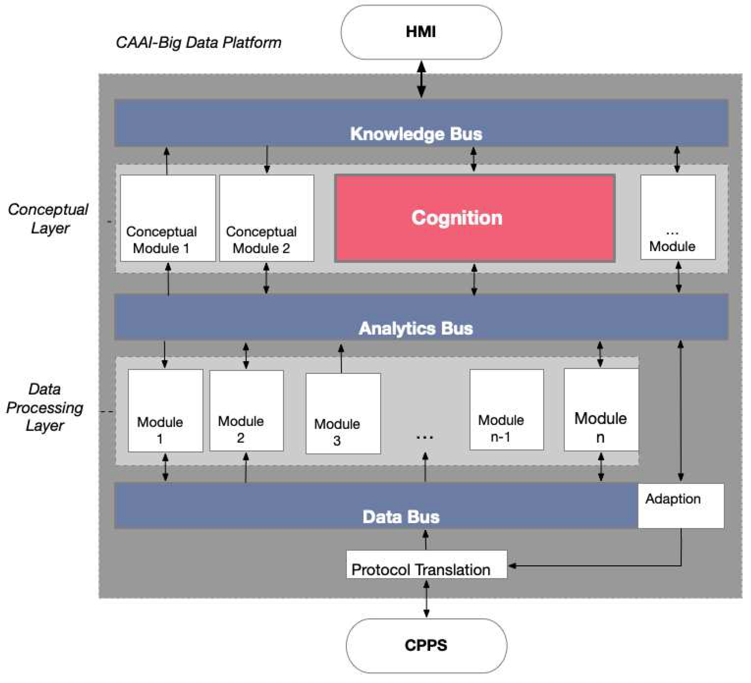
The idea of the KOARCH project was to develop an architecture that meets these requirements, based on a BDP. This BDP is mapped in Figure 1. By looking at the structure of the architecture, it can be seen that the different components are realized via different modules. This modularization of the CAAI allows for flexible adaptation or extension. A virtualized container is used for every module or component of the BDP. Kubernetes is used as a framework to orchestrate the different micro-services. The BDP is divided into two main layers: the conceptual layer and the data processing layer. The modules of these layers communicate via three different buses. Raw data from the CPPS, demonstrators, or external simulation modules enter the BDP via the data bus. Cleaned and preprocessed data are transported back to the data bus by the preprocessing module to be forwarded to other modules of the data processing layer. The analytics bus ensures connection between modules of the data processing layer and the conceptual layer. Results transmitted here have significantly higher information density than those from the data bus. The most influential component is the cognition module, located in the conceptual layer. It compiles pipelines for suitable algorithms based on overall goals and boundary conditions. The knowledge bus is responsible for communication between the Human-Machine Interface (HMI) and the conceptual layer, transmitting user commands and goals as well as reports of the process and results to the user.

The idea is that the users can define one or more higher-level goals such as optimization, anomaly detection, predictive maintenance, etc. Additionally, they can establish constraints for the process. These constraints include the definition of signals that the algorithm utilizes as features for the respective algorithm, as well as limits for the associated values. Moreover, target-dependent settings can be configured. For instance, in an optimization application, the objective function and the optimization goal (minimization or maximization) can be specified.

During the subsequent step, the cognitive module forms processing pipelines based on the selected objective. It selects appropriate preprocessing steps and algorithms. For decision making, the cognitive module relies on simulation data and experience from similar, previously developed applications. Moreover, SMBO has been implemented to achieve maximum performance of the algorithms.

The evaluation of the architecture was performed using a versatile production system (VPS). This VPS is located in a laboratory of the Ostwestfalen-Lippe University of Applied Sciences (TH OWL). The VPS is a modular production system that processes corn to produce popcorn and package it. During the retrospective evaluation of the architecture, it became apparent that the CAAI performs well for fixed tasks. However, an individual implementation effort is still required for each use case. These findings will be detailed in a forthcoming paper.

During the detailed analysis of the architecture, it was observed that a critical category of algorithms, namely OML algorithms, had not been incorporated in the implementation. The configuration of the CPPS creates an ideal environment for the deployment of OML algorithms. The production system machinery generates continuous streams of data. Implementing OML strategies would mean these vast quantities of data would not need to be stored, alleviating storage demands. Furthermore, the system could flexibly and swiftly adapt to concept drifts. Therefore, the primary focus of this article is to evaluate the potential and effectiveness of integrating OML algorithms within the CPPS context and to demonstrate the importance of integrating OML-capabilities into the CAAI-framework.

2.2. The Need for Online Machine Learning

The volume of data generated from various sources has increased enormously in recent years ("Big Data"). Technological advances have enabled the continuous collection of data. Sensor data, web data, social media data, share prices, search queries, clickstream data, operational monitoring data, online advertising, mobile data and the Internet of Things data are referred to as streaming data. Streaming data, or streams of data, is an infinite and continuous flow of data from a source, often arriving at very high speeds. Therefore, streaming data is a subset of Big Data. In addition to the increased frequency, streaming data and static data also differ in that the former have less structure. Streaming data is loosely structured, volatile (only available once) and always "flowing" data. It requires real-time or near real-time analysis. Since the data stream is constantly being produced and never ends, it is not possible to store this enormous amount of data and only then carry out analyzes on it (as with batch data).

The classical BML approach, which boils down to the following [8]:

Loading and pre-processing the train data;
Fitting a model to the data;
Calculating the performance of the model on the test data;

has certain disadvantages. Batch learning models are not suitable for handling streaming data, since multiple passes over the data are not possible. The batch models may soon become outdated due to concept drifts (i.e. data distribution changes over time). Furthermore, BML has problems regarding storage requirements, unknown data, and accessibility of data, which will be discussed next.

For example, in the case of energy consumption forecast, the previously known consumption values are only one element that is required for the modelling. In practice, future demand is driven by a range of non-stationary forces—such as climate variability, population growth, or disruptive clean energy technologies—that may require both gradual and sudden domain adjustment. Therefore, prediction, classification, regression, or anomaly detection approaches should be able to detect and respond to conceptual deviations in a timely manner so that the model can be updated as quickly as possible. Although BML models can be retrained regularly, this is infeasible in many situations because the training is too expensive.

Another problem for BML is that it cannot incorporate new data containing unknown attributes. When new data is made available, the model has to be learned from scratch with a new dataset composed of the old data and the new data. This is particularly difficult in a situation where new data and attributes come in every day, every hour, every minute or even with every measurement like it is the case for production processes.

The enormous amount of data can lead to another problem when the dataset size exceeds the available amount of RAM. Possible solutions include the optimization of data types (sparse representations), the usage of a partial data set ("out-of-core learning"), i.e., the data is divided into blocks or mini-batches, or the application of highly simplified models.

Last but not least, data accessibility is a problem for BML: each time the BML model is trained, features must be extracted. The problem is that some features are no longer available after some time, e.g. because they were overwritten or simply deleted. This means that features that were still available last week, may no longer be available at the current time. In general, it is not always possible to provide all data at the same time and in the same place. In addition to these issues, BML and especially deep learning algorithms can cause high energy costs.

The challenges of streaming data led to the development of a class of methods known as incremental or online learning methods. The introduction of different methods of online learning/incremental learning has been quite slow over the years, but the situation is changing at the moment [9] [10] [11]. The point of incremental learning is to fit an ML model to a data stream. In other words, the data are not available in their entirety, but the observations are provided one at a time. This way, the models can be updated incrementally before the data is discarded. The axioms for stream learning, which form the foundation of OML, can be derived from the following requirements [10]:

Each instance can only be used once;
The processing time is severely limited;
The memory is limited ("sublinear in the length of the stream");
The algorithm must be able to deliver a result at any time ("anytime property");
Data streams are assumed to change over time, i.e. the data sources are not stationary;

2.2.1. OML Methods

There are many ML models that can be adapted to OML implementations. For example, online linear regression is a popular method in OML. Stochastic gradient descent (SGD) is used to update the coefficients in the implementation of an online linear regression model, as not all data is available at once. SGD is commonly used to train neural networks.

Tree-based algorithms are also popular in OML. Trees have nodes for testing attributes, usually by comparison, and branches for storing the test results and making predictions (of a class in classification or a value in regression). One challenge with streaming data is the high storage requirements, as it is impossible to save all data. Trees allow for compact representation, making them popular methods in OML. A BML tree reuses instances to calculate the best splitting attributes (“splits”). Therefore, using BML decision tree methods like Classification And Regression Tree (CART) is not effective in a streaming data context. Instead, Hoeffding trees are used in OML. They do not reuse instances but wait for new instances to arrive [12]. As an incremental decision tree learner, a Hoeffding tree is better suited to a streaming data context. It is based on the idea that a small sample is often sufficient to select an optimal splitting attribute, supported by the statistical result known as the Hoeffding bound. The Hoeffding tree converges to a tree generated by a BML algorithm with sufficiently large data [10]. However, streaming data can be very noisy, affecting performance (in terms of prediction accuracy) and potentially generating very large trees. Several extensions of the basic Hoeffding tree exist, such as Hoeffding Anytime Trees that work similarly but use a modified splitting procedure.

The Hoeffding Adaptive Tree (HAT) [13] is an extension of the Hoeffding Tree, incorporating a mechanism for identifying concept drift. It employs an instance of the ADWIN [14] concept-drift detector at each decision node to monitor potential shifts in data distribution.

2.2.2. The Evaluation Frame: How to Compare the Methods

To compare OML with classical approaches and to evaluate the strengths and weaknesses of various forecasting methods, different approaches were employed in our experiments. Three distinct methods were used to generate the training dataset for batch procedures. In order to provide a detailed explanation of these methods, it is important to first describe the experimental procedure. The objective of each method was to produce point forecasts with maximum accuracy for a predetermined horizon of 150 data points in the future. However, the development of models differed among the methods. For batch procedures, a classical train-test split was used, referred to as "batch" hereafter, along with a train-test split using a landmark approach and a train-test split with a shifting window. Additionally, the OML approach was utilized for model development. The evaluation functions eval_bml, eval_bml_landmark, eval_bml_window, and eval_oml_horizon accept two data frames as arguments:

train, denoted as $D_{train}$ , with size $s_{train}$ , is used to fit the model.
test, denoted as $D_{test}$ , with size $s_{test}$ , is used to evaluate the model on new (unseen) data.

First, the method eval_bml implements the "classical" BML approach. The algorithm is trained once on the training data set, resulting in a model, denoted as

M_{bml}

, that is not modified. The model

M_{bml}

is evaluated on the test data, where the horizon, denoted as

h \in [1, s_{test}]

, specifies the size of the partitions that

D_{test}

is split into. If

h = s_{test}

, then the basic ML train-test setting is implemented. If

h = 1

, an OML setting is simulated.

Second, the method eval_bml_landmark implements a landmark approach. The first step is similar to that of the BML approach, resulting in an initial model

M_{bml}^{(1)}

. However, subsequent steps differ: after making a prediction with

M_{bml}^{(1)}

for the batch of data instances from the interval

[s_{train}, s_{train} + h]

, the algorithm is retrained on the interval

[1, s_{train} + h]

to produce an updated model

M_{bml}^{(2)}

. During the third step of the landmark BML approach,

M_{bml}^{(2)}

makes predictions for

[s_{train} + h, train + 2 \times h]

and a new algorithm

M_{bml}^{(2)}

is trained on

[1, train + 2 \times h]

Third, the method eval_bml_window implements a window approach. Again, the first step is similar to that of the BML approach, resulting in an initial model

M_{bml}^{(1)}

. Subsequent steps are similar to those of the landmark approach with one important exception: instead of being trained on the complete set of seen data, the algorithm is trained on a moving window of size

s_{train}

Finally, the method eval_oml_horizon implements an OML approach. This approach differs fundamentally from BML approaches because every single instance is used for both prediction and training. If

h = 1

, a "pure" OML algorithm is implemented. If

h > 1

, OML computations are performed h times.

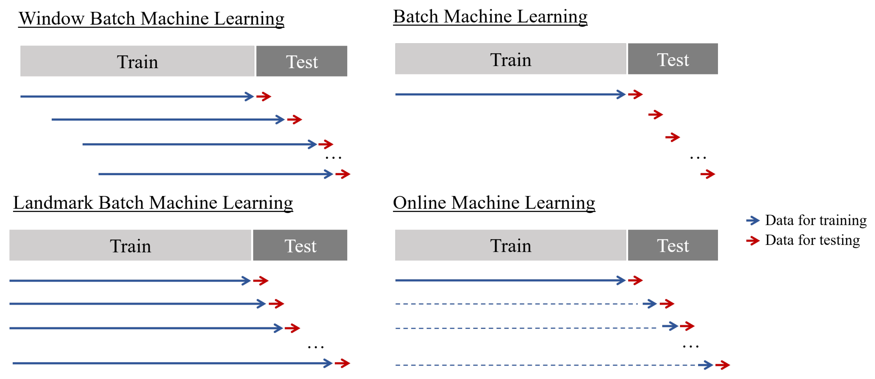
A summary of the training and test set generation process, related to the corresponding evaluation procedure, can be found in Table 5 in the appendix. Additionally, Figure 2 visualizes the differences between the evaluation techniques introduced. Several criteria are used to evaluate the different approaches, including Mean Absolute Error (MAE), computation time, and memory consumption. The selection of these metrics is based on the different requirements that an end user might have for the system. While the model with the lowest error is preferred, computation time can be a crucial factor in high-frequency data, and memory consumption should not be ignored, as more complex models can take up several gigabytes. By memory consumption, we do not mean an exact calculation of the size of the model, but measurements of peak memory consumption during the model’s training and testing processes. This approach allows us to conveniently compare the memory consumption of ML algorithms from different Python packages (Sklearn and River). All evaluation methods described in this section are available in the open-source spotRiver package on GitHub2

2.2.3. Real World Application: Slitting Machines

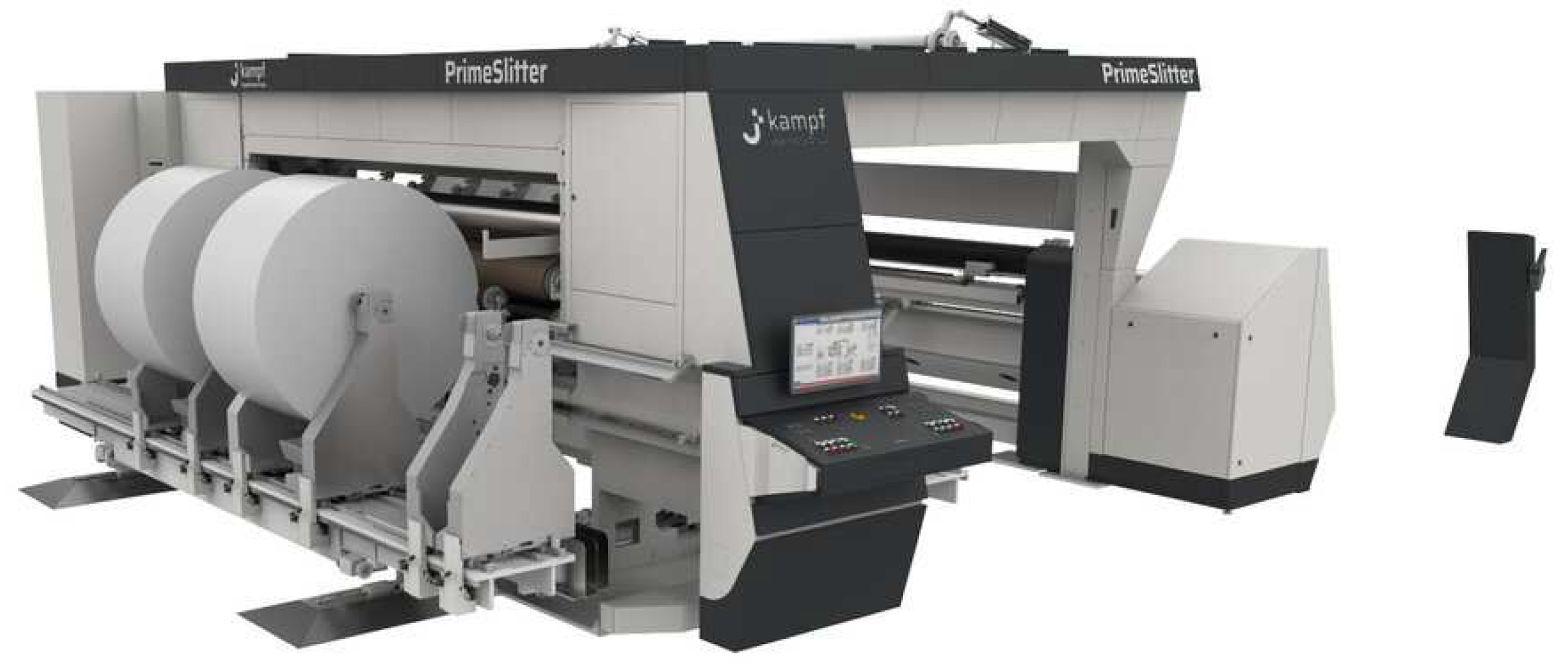
In the experiments discussed in this work, data were collected using a test setup for winding stations from "Kampf Schneid- und Wickeltechnik GmbH & Co. KG", a company that specializes in building machines for slitting and winding web-shaped materials such as paper, plastic films, or aluminum foil, as depicted in Figure 3. A paper core is secured between two winding stations to wind the web into a roll, achieving a diameter of up to 1500 mm and weights of up to 6 tons. The necessary web tension for different materials is maintained by a drive, which adjusts to compensate for the increasing diameter.

The test setup facilitated the evaluation of new concepts for winding stations and helped in determining the lifespan of various components including bearings and belts. Additional sensors were installed to monitor temperatures and vibration levels at different points, enabling a more comprehensive analysis of their behavior. In one of the trials, a machine run to wind up a representative material was simulated under defined conditions including parameters such as material thickness, material density, material width, induced tension, machine speed, and acceleration and deceleration times, in addition to core and finished diameters.

The collected time-series data encapsulates information regarding motor temperature, revolutions, and torques, as well as data from external sensors monitoring temperature and vibration levels. For the experiments outlined in this article, only specific data were utilized: motor revolution [

\frac{1}{\min}

], motor torque [Nm], and the vibration data at a particular point. The vibration data is measured in analog values between 0 and 27,648 related to a range between 0 - 25 [

\frac{m m}{s^{2}}

]. Motor revolution and torque are used as input features while the vibration level is the prediction target. Data was logged every one hundredth of a second, with each timestamp recording the respective feature values. To simulate external influences such as roll handling or other factory operations, further vibrations were introduced intermittently by gently hitting and shaking the winding stations.

In our experiments, the data provided by Kampf Schneid- und Wickeltechnik GmbH & Co. KG was utilized to predict the vibration of level station 1 using motor revolution and torque. A forecast horizon of t = 150 was defined. This horizon refers to the time when the models will be updated again. For instance, in this experiment, the models were updated after collecting 150 data points although each approach employed a distinct strategy. The classic batch method did not update the model and only utilized training data. The batch approach with a landmark strategy included newly collected data in the training data and created a new model on the enlarged dataset. On the other hand, the batch model with a shifting window approach excluded the first 150 data points of the training set and appended each new 150 data points to the end of the training data. A new model was then produced based on this new dataset ensuring that the length of the training data set remained constant. Finally, in the OML approach, 150 data points were collected and sequentially passed to the model.

In the batch approaches, a Decision Tree Regressor from the sklearn package [15] was utilized while Hoeffding Tree Regressor (HTR) from the river package [16] was used in the OML approach. Before passing data to regressor it was standardized. For the initial training of the models 1,462,555 samples are used. The subsequent evaluation horizon consists of 30,196 data points. This test set includes four potential future evolutions of the vibration level. Figure 4 displays the temporal evolution of vibration observed in one test scenario, revealing distinct local peaks followed by sharp drops and subsequent slow recovery before the emergence of new peaks.

2.3. Hyperparameter Tuning

The goal of HPT is to optimize the hyperparameters in a way that improves the performance of a ML model. This is an important but usually difficult and computationally intensive task. The simplest approach, but also the most computationally expensive, is manual search (or trial-and-error) [17].

Common approaches include simple random search (RS), where hyperparameters are randomly and repeatedly selected for evaluation, and grid search. Directed search methods and other model-free algorithms, such as evolution strategies [18] or pattern search [19], also play an important role. Hyperband, a multi-armed bandit strategy that dynamically allocates resources to a set of random configurations and uses successive bisections to stop configurations with poor performance [20], is also commonly used in the HPT domain. The most sophisticated and efficient approaches are Bayesian Optimization (BO) and SMBO methods, which are based on the optimization of cost functions obtained through simulations or experiments.

In this article, we consider an HPT approach based on the Sequential Parameter Optimization Toolbox (SPOT) [21], which is suitable for situations where only limited resources are available. This may be due to limited availability or cost of hardware. Another reason might be that confidential data may only be processed locally due to legal requirements. Furthermore, our approach emphasizes the importance of understanding algorithms as a key tool for transparency and explainability. This can be enabled by quantifying the contribution of ML and Deep Learning components (nodes, layers, split decisions, activation functions, etc.) and understanding the meaning of hyperparameters and their interactions. SPOT provides statistical tools for understanding hyperparameters and their interactions. Additionally, the SPOT software code is available in the open-source spotPython and spotRiver packages on GitHub3, allowing for replicability of results. SPOT is an established open-source software that has been maintained for over 15 years [21] [22]. It includes SMBO methods for tuning based on classical regression and analysis of variance techniques, tree-based models such as CART and RF, BO (Gaussian Process Models, also known as Kriging), and combinations of different meta-modeling approaches. Any ML model in scikit-learn (sklearn) can be used as a meta-model.Details on SPOT and its application in practice are given by [23].

The loop of the model based tuning process with SPOT can be devided into the following steps [24]:

Setup: Different combinations of hyperparameter values are evaluated in order to build an initial design.
Evaluation: The new or initial hyperparamters are evaluated.
Termination: The loop checks weather a termination criterion like maximum number of iteration or maximum tuning time has been reached.
Selection: This step selects samples for building the surrogate model.
Building Surrogate: The surrogate is build.
Surrogate Search: The algorithm searches for the best hyperparameter settings based on the surrogate model.
Optimal Computing Budget Allocation (OCBA): This step is used to determine the number of repeated evaluation.

2.3.1. SMBO Tuning Setup

In order to find the optimal parameters for the HRT algorithm, we employ Gaussian Process Regression (GPR) [25] as a surrogate model in the context of SMBO. GPR, also known as Kriging model, is the default surrogate choice for SMBO within the SPOT framework. To drive this optimization process, we have chosen the Differential Evolution (DE) [26] algorithm as our optimization method.

The optimization bounds, along with the default values assigned to the tuned hyperparameters, are outlined in Table 2. Notably, the optimization process is time limited, with a maximum duration of 100 minutes. It is important to emphasize that this countdown starts only after the initialization of the initial surrogate model design, which in our specific case consists of 50 data points. Due to the fact that our dataset is very large (almost 1.5 million samples) we use only 2% of trainings and test set for HPT. The remaining data is subsequently used for the actual training and evaluation of the tuned and default model. The goal of the optimization is to minimize a combined value of MAE, computation time, and memory usage. These values are weighted differently (MAE: 1, memory consumption: 1e-3, calculation time: 1e-3).

3. Results

3.1. Real World Application Results

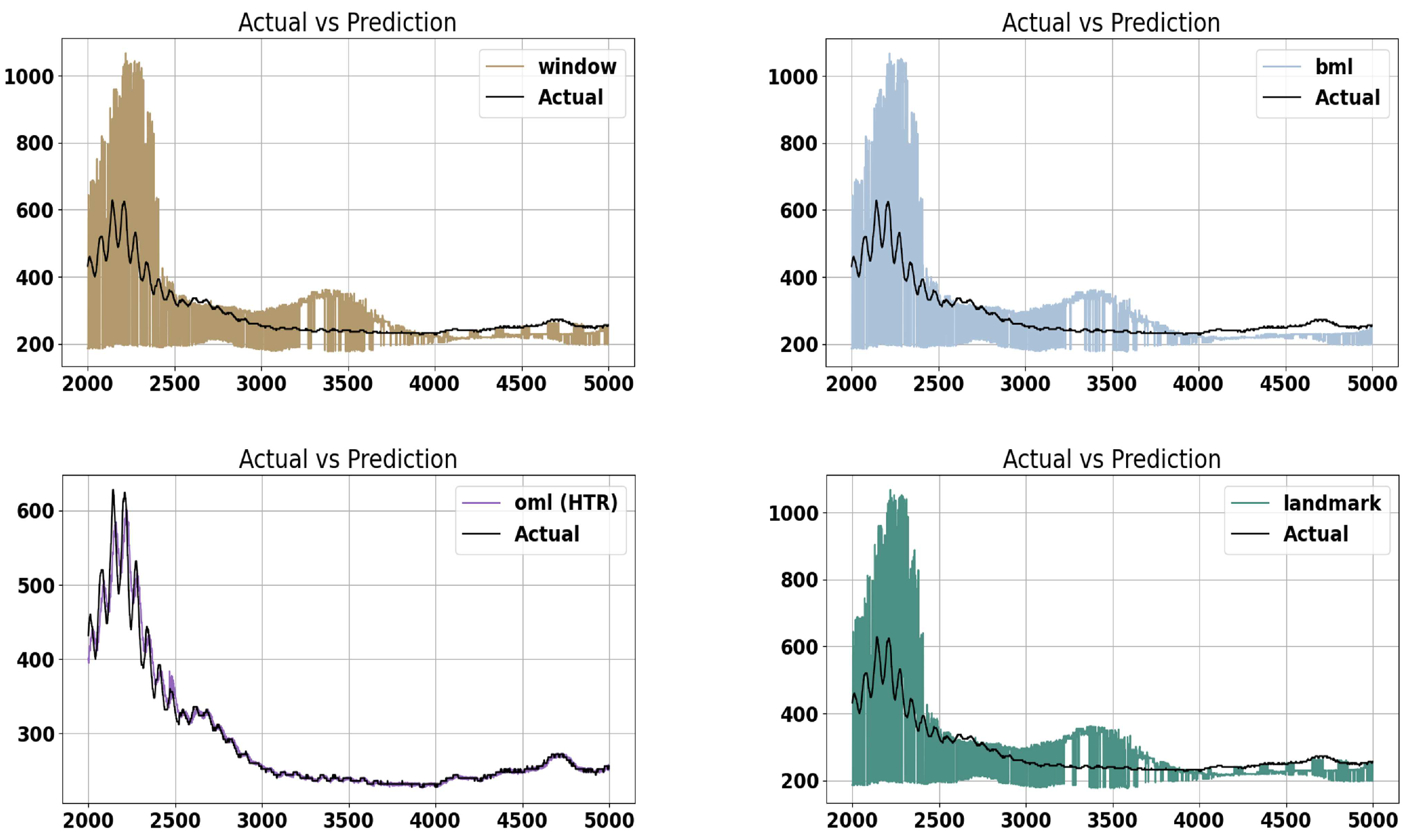
This chapter presents the results of the different evaluation procedures, which were presented in Section 2.2.2. In Figure 5, we see a comparison between model predictions and actual values. To look at the behavior of the methods in more detail, the graph refers only to a window of 3,000 data points. All three BML methods consistently overshoot actual values, while the OML algorithm generally provide accurate predictions. The first 500 predictions show clear oscillations of the actual values. Especially with these data points, batch learning evaluation methods have difficulty making usable predictions. It is clear to see how the OML algorithm responds flexibly to the fluctuations and delivers accurate predictions.

3.1.1. Evaluation Metric

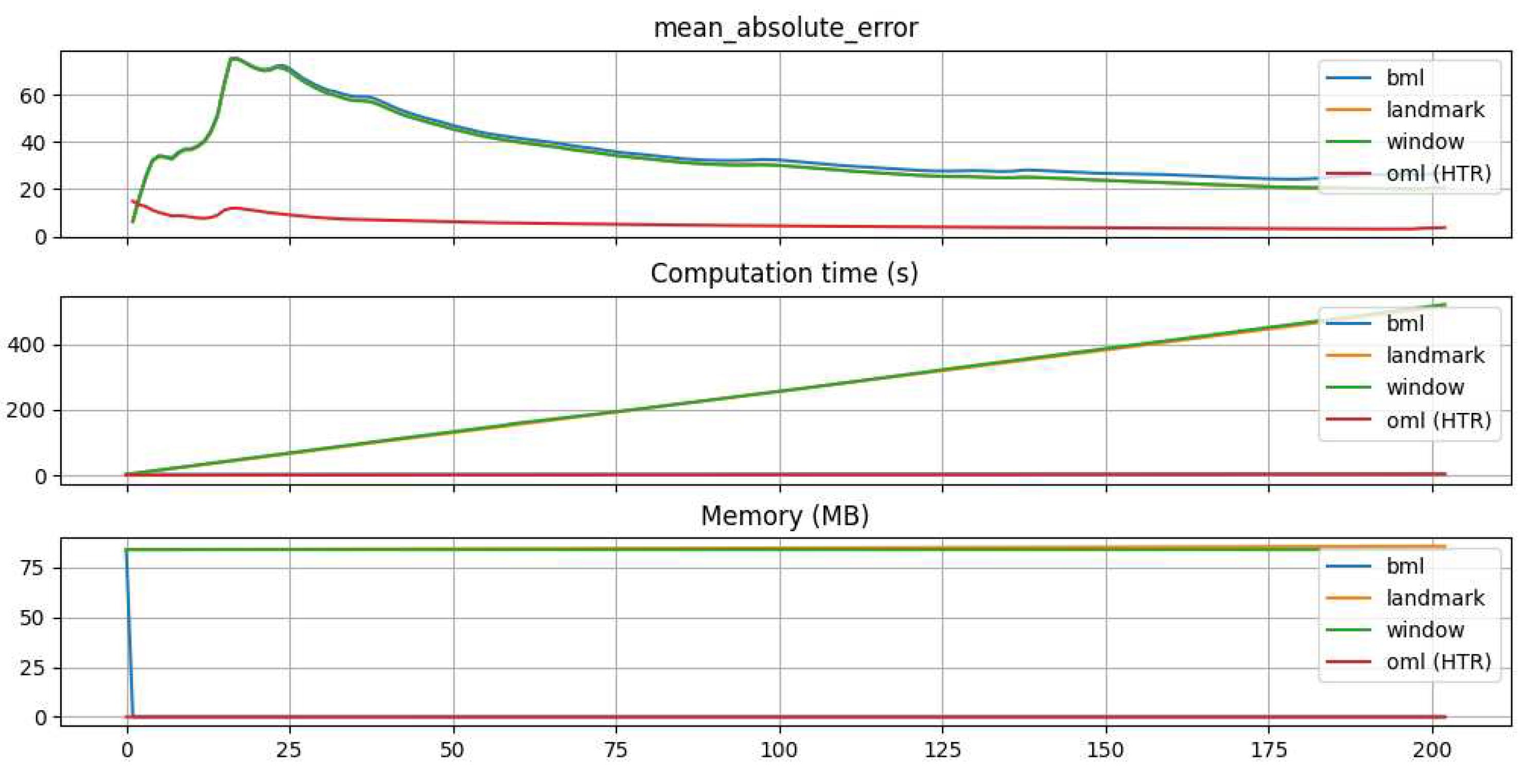
The performance of the different approaches is visualized in the top graph of Figure 6. It shows how the MAE evolves over the evaluation horizon. All batch learning evaluation methods produce comparable results. Initially, performance degrades slightly and then improves continuously. The OML approach comparatively achieves constant results and outperforms the batch evaluations over the entire horizon.

3.1.2. Computation Time

The second diagram in Figure 6 shows a comparison of the computation times of the different methods. As assumed, the landmark and shifting-window methods show a continuous increase in computation time due to the models need to be retrained at each evaluation iteration. In contrast, the conventional batch learning approach exhibits a much lower processing time because of its singular model training phase. On the other hand, the OML algorithm achieves time efficient results as well. This is because OML updates models incrementally, rather than training from scratch with each evaluation.

3.1.3. Memory Consumption

The lowest graph of Figure 6 shows the memory consumption. Here, the OML approach also delivers comparable results to the basic batch approach. However, it should be emphasized again that the batch approach’s memory consumption only takes place during the training step, and the remaining consumption is negligible. This fact is also visualized by the graph. In the first evaluation step, the memory consumption for the classic batch method drops towards zero. The shifting window and the landmark approach perform comparably poorly. This is mainly due to the generated model, which must be built again in each iteration.

3.1.4. Statistical Evaluation

Given that graphical evaluations alone may not be sufficient, a statistical evaluation was conducted to determine whether there was a significant difference in the mean deviation of the differences between the prediction and true values of two time series. This approach aimed to ascertain whether one of the time series provided a better approximation of the true time series by examining if the mean difference of one time series was significantly smaller than the other. To perform the statistical analysis, the procedure of [27] was used.

Our process involved selecting two time series for comparison, where time series one was always the OML approach and time series two was one of the remaining methods. Next, the number of samples required to make an informed decision was calculated under the following assumptions:

$α = 0.05$ - Probability of a Type I error, known as a false positive.
$β = 0.2$ - Probability of a Type II error, known as a false negative; $1 - β$ is known as the power of the test.
$σ =$ Standard deviation of the difference of the absolute differences between model 1 and model 2.
$Δ =$ Twice the mean value of the absolute deviation between the actual values and the output of the OML approach.

Instead of considering each sample value individually, we consider the overall mean of the absolute deviation between the prediction and the true value from each time series. It was determined that between 518 and 527 samples were needed, depending on the time series. Since the analyzed time series comprised around 30,000 samples, obtaining the required sample size was not problematic.

In the third step, a one-sided t-test was conducted, using the difference of the absolute values between the two time series. We formulated the following hypothesis, where j denotes the index of either the batch, landmark, or shifting window approach:

\begin{matrix} H_{0} : μ_{O M L} - μ_{j} & \geq 0 \\ H_{1} : μ_{O M L} - μ_{j} & < 0 \end{matrix}

Based on the analysis, it was concluded that the null hypothesis could be rejected in all cases, indicating that the mean deviation of the differences of the OML approach was significantly smaller than that of all other approaches.

3.2. Hyperparameter Tuning Results

This section highlights the results of the HPT process. Figure 7 shows the progress of the tuning process. The initial design phase is represented by the 50 black data points on the left side of the graph. Each point represents the result of the evaluation at different stages of our initial design phase. The more data points that are evaluated for the initial design, the more accurate our surrogate model will be at the start of the optimization process. The continuous red line that follows the initial points traces the trajectory of the best hyperparameter setup found so far within the tuning progresses. It can be seen that the value of the objective function could be reduced after initialization through optimization.

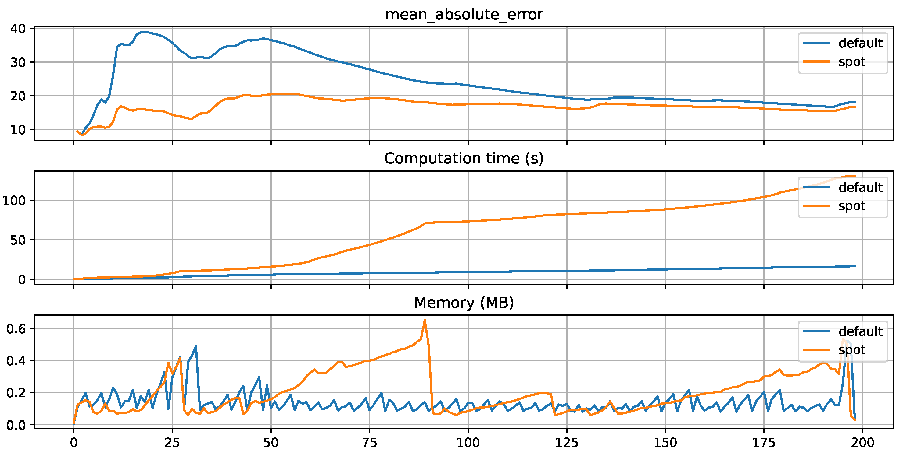
Figure 8 illustrates the comparison of results over the entire evaluation horizon in terms of MAE, computation time, and memory consumption between the tuned model and the model with default parameters. It is evident that the tuned model consistently outperforms the default algorithm in terms of MAE throughout the evaluation period. However, it is noteworthy that the tuned model consumes more computation time and memory resources than the default model. This can be explained by the fact that, as explained in 2.3.1, the weighting of the MAE in this particular tuning run is significantly higher than the weighting of the time and memory consumption.

To statistically prove the improvement in performance with respect to the metric, a one-one-sided t-test, like explained in Section 3.1.4, is performed again with the following hypothesis:

\begin{matrix} H_{0} : μ_{H T R_{t u n e d}} - μ_{H T R_{d e f a u l t}} \geq 0 \\ H_{1} : μ_{H T R_{t u n e d}} - μ_{H T R_{d e f a u l t}} < 0 \end{matrix}

The result of the t-test states that the zero hypthosis is rejected. This means that the average deviations of the predictions of the tuned model are significantly lower than those of the default model.

The increase in computation time and memory consumption can be attributed to the values of the tuned parameters. Table 3 presents a comparison between the tuned and default values for each hyperparameter, along with their respective importance as determined during spot optimization. It is evident that the Leaf Model and the Prediction function of the leaves exert the most significant influence on the evaluation outcomes. Upon contrasting the tuned and default values, the reasons behind the higher memory consumption and computation time in the tuned model become apparent. Specifically, the grace period, set at a value of 12, notably deviates from the default model’s value of 200. Consequently, a considerably greater number of splits occur in the tuned model.

3.2.1. Hyperparameter Tuning for Improving Time and Memory Consumption

In production processes, certain conditions may necessitate the optimization of algorithms with respect to time and memory consumption. These conditions may include a requirement for near real-time capability, limited RAM capacities, or the need to conserve energy. Consequently, we conducted an overhead experiment to demonstrate that the HTR can be optimized for these two criteria using SPOT. We adjusted the weightings as described in Section 2.3.1 to prioritize optimization (MAE:1, memory consumption:10, calculation time: 10).

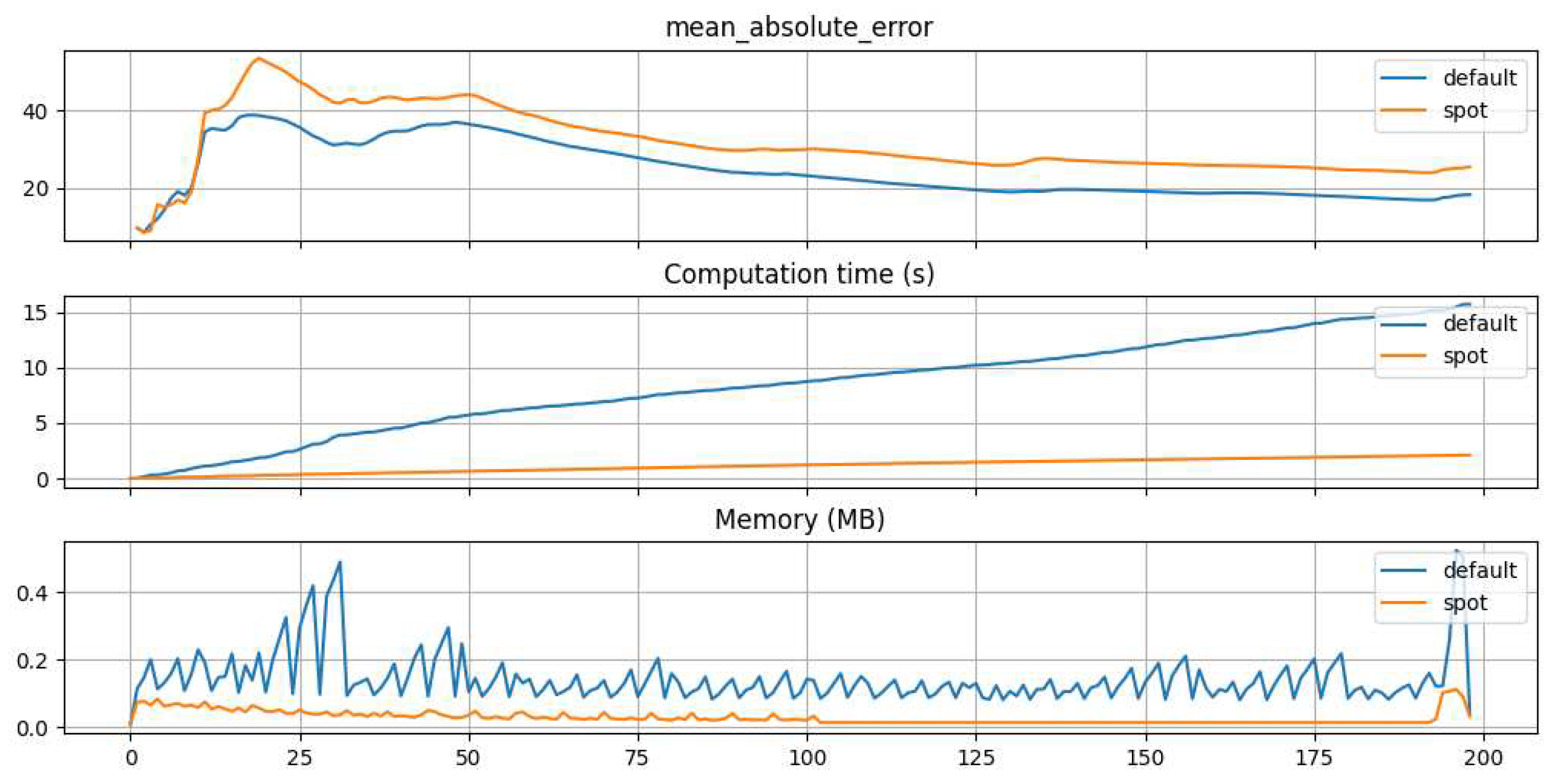
Figure 9 illustrates that, over the entire evaluation horizon, the computation time and memory consumption of the tuned model are significantly lower than those of the default model. However, it is also evident that the tuned model exhibits a higher deviation in the predictions of vibration development due to the altered optimization priority.

This behavior can be elucidated by examining Table 4. It is apparent that the grace period is nearing the upper boundary established in the tuning process. Consequently, the splitting process of the leafs is not executed as frequently as for the untuned model, thereby conserving computational resources. Moreover, the maximum depth of the tree at a value of four is markedly lesser than the default setting of the algorithm, which stands at 20. This further contributes to the reduction in computational effort and memory usage.

4. Discussion

In this study, we revisited the CAAI developed in the KOARCH project. During the revision of this architecture, we briefly noted the existing limitations in automating the algorithm pipeline development process for all environments and use cases. This is mainly due to rapidly changing software interfaces and transfer complexities. While this highlights the need for some human intervention, our focus quickly shifted to exploring the potential of OML in the context of production processes. Our attention centered on the notable absence of OML technology in the current CAAI-framework, especially given the continuous data streams in CPPS. To illustrate the benefits of OML in industrial setups, we conducted experiments using a slitting machine setup. During testing, we compared the OML approach against three BML based methods. The OML approach significantly outperformed the BML strategies, primarily due to its ability to update models iteratively, allowing for a swift response to concept drift in data. This feature is especially useful in machinery and predictive maintenance applications, presenting a more efficient alternative. Furthermore, the OML approach demonstrated computational benefits, showing not only time efficiency but also conservative memory usage. The performance was notably better than that of the other two methods, where the models were retrained following the initial training, namely the shifting window and landmark strategies. In order to optimize the OML algorithm’s performance, we introduced SMBO to identify the best hyperparameter sets. Using SPOT for hyperparameter tuning significantly improved algorithm performance. Additionally, adjusting the priorities during the optimization phase successfully optimized computation time and memory consumption. In conclusion, this study underscores the potential of integrating OML technology and the effectiveness of hyperparameter tuning in enhancing CPPS. This research paves the way for the development of more agile and efficient cyber-physical production systems, ready to tackle the dynamic demands of industrial operations with refined precision and adaptability.

Author Contributions

This paper was supervised by Alexander Hinterleitner, Richard Schulz and Thomas Bartz-Beielstein. These three authors contributed equally to all the tasks. They were assisted in the following subtasks by the following authors: Validation of the approach was performed by Lukas Hans, Phillip Priss and Christoph Geng. Software was developed by Noah Pütz, Nils Barthel, Aleksandr Subbotin and Lukas Hans. Data Curation was performed by Aleksandr Subbotin and Nils Barthel. Writing was supported by Lukas Hans and Martin Rosellen. All authors have read and agreed to the published version of the manuscript.

Funding

This research work is funded by the German Federal Ministry for Economic Affairs and Climate Action as part of the project “IMProvT_II -– Intelligente Messverfahren zur energetischen Prozessoptimierung von Trinkwasserbereitstellung und -verteilung II”, funding code 03EN2086A.

Institutional Review Board Statement

Not applicable

Informed Consent Statement

Not applicable.

Data Availability Statement

The data presented in this study are available on request from the corresponding author. The data are not publicly available due to confidentiality restrictions.

Conflicts of Interest

The authors declare no conflict of interest.

Abbreviations

The following abbreviations are used in this manuscript:

BDP	Big Data Platform
BML	Batch Machine Learning
BO	Bayesian Optimization
CAAI	Cognitive Architecture for Artificial Intelligence
CART	Classification and Regression Tree
CPPS	Cyber Physical Production System
DE	Differential Evolution
EFDT	Extremely Fast Decision Trees
GPR	Gaussian Process Regression
HAT	Hoeffding Adaptive Tree
HMI	Human Machine Interface
HPT	Hyperparameter Tuning
HTR	Hoeffding Tree Regressor
OML	Online Machine Learning
RF	Random Forest
SGD	Stochastic Gradient Descent
SMBO	Surrogate Model Based Optimization
SPOT	Sequential Parameter Optimization Toolbox
VPS	Versatile Production System

5. Appendix

Table 5. Evaluation methods. Batches are denoted as intervals, e.g.,

[a, b]

. The OML approach passes every instance from the interval to the online algorithm separately for prediction and update (training).

Table 5. Evaluation methods. Batches are denoted as intervals, e.g.,

[a, b]

. The OML approach passes every instance from the interval to the online algorithm separately for prediction and update (training).

Name	Step	Training interval / instances	Training batch size	Model	Prediction interval
BML ("Classical")	1	$[1, s_{train}]$	$s_{train}$	$M^{(1)}$	$[s_{train} + 1, s_{train} + h]$
	n	$[1, s_{train}]$	0	$M^{(1)}$	$[s_{train} + (n - 1) \times h + 1, s_{train} + n \times h]$
Landmark BML	1	$[1, s_{train}]$	$s_{train}$	$M^{(1)}$	$[s_{train} + 1, s_{train} + h]$
	n	$[1, s_{train} + (n - 1) \times h]$	$s_{train} + (n - 1) \times h$	$M^{(n)}$	$[s_{train} + (n - 1) \times h + 1, s_{train} + n \times h]$
Window BML	1	$[1, s_{train}]$	$s_{train}$	$M^{(1)}$	$[s_{train} + 1, s_{train} + h]$
	n	$[1 + (n - 1) \times h, s_{train} + (n - 1) \times h]$	$s_{train}$	$M^{(n)}$	$[s_{train} + (n - 1) \times h + 1, s_{train} + n \times h]$
OML	1	$[1, s_{train}]$	1	$M^{(1)}$	$[s_{train} + 1, s_{train} + h]$
	n	$[1, s_{train} + (n - 1) \times h]$	1	$M^{(n)}$	$[s_{train} + (n - 1) \times h + 1, s_{train} + n \times h]$

References

Adolphs, P.; others. Reference Architecture Model Industrie 4.0 (RAMI4.0). Tech. rep., VDI, 2015.
Lin, S.W.; others. The Industrial Internet of Things Volume G1: Reference Architecture v1.80. Technical report, Industrial Internet Consortium, 2017.
Lee, J.; Jin, C.; Bagheri, B. Cyber physical systems for predictive production systems. Production Engineering 2017, 11, 155–165. [CrossRef]
Laird, J.E.; Newell, A.; Rosenbloom, P.S. SOAR: An Architecture for General Intelligence. Artif. Intell. 1987, 33, 1–64. [CrossRef]
Anderson, J.R. A Simple Theory of Complex Cognition. American Psychologist 1996. [CrossRef]
Fischbach, A.; Strohschein, J.; Bunte, A.; Stork, J.; Faeskorn-Woyke, H.; Moriz, N.; Bartz-Beielstein, T. CAAI—a cognitive architecture to introduce artificial intelligence in cyber-physical production systems. The International Journal of Advanced Manufacturing Technology 2020, 111, 609–626. [CrossRef]
Bunte, A.; Fischbach, A.; Strohschein, J.; Bartz-Beielstein, T.; Faeskorn-Woyke, H.; Niggemann, O. Evaluation of Cognitive Architectures for Cyber-Physical Production Systems. 24th IEEE International Conference on Emerging Technologies and Factory Automation, ETFA 2019, Zaragoza, Spain, September 10-13, 2019, 2019, pp. 729–736. [CrossRef]
Bartz-Beielstein, T.; Zaefferer, M.; Mersmann, O. Tuning: Methodology. In Hyperparameter Tuning for Machine and Deep Learning with R - A Practical Guide; Bartz, E.; Bartz-Beielstein, T.; Zaefferer, M.; Mersmann, O., Eds.; Springer, 2022; chapter 2, pp. 7–26. in print.
Montiel, J.; Halford, M.; Mastelini, S.M.; Bolmier, G.; Sourty, R.; Vaysse, R.; Zouitine, A.; Gomes, H.M.; Read, J.; Abdessalem, T.; others. River: machine learning for streaming data in Python 2021.
Bifet, A.; Gavalda, R.; Holmes, G.; Pfahringer, B. Machine Learning for Data Streams with Practical Examples in MOA; MIT Press, 2018. https://moa.cms.waikato.ac.nz/book.
Losing, V.; Hammer, B.; Wersing, H. Incremental on-line learning: A review and comparison of state of the art algorithms. Neurocomputing 2018, 275, 1261–1274. [CrossRef]
Domingos, P.M.; Hulten, G. Mining high-speed data streams. Proceedings of the sixth ACM SIGKDD international conference on Knowledge discovery and data mining, Boston, MA, USA, August 20-23, 2000; Ramakrishnan, R.; Stolfo, S.J.; Bayardo, R.J.; Parsa, I., Eds. ACM, 2000, pp. 71–80. [CrossRef]
Bifet, A.; Gavalda, R. Adaptive learning from evolving data streams. Advances in Intelligent Data Analysis VIII: 8th International Symposium on Intelligent Data Analysis, IDA 2009, Lyon, France, August 31-September 2, 2009. Proceedings 8. Springer, 2009, pp. 249–260.
Bifet, A.; Gavalda, R. Learning from time-changing data with adaptive windowing. Proceedings of the 2007 SIAM international conference on data mining. SIAM, 2007, pp. 443–448.
Pedregosa, F.; Varoquaux, G.; Gramfort, A.; Michel, V.; Thirion, B.; Grisel, O.; Blondel, M.; Prettenhofer, P.; Weiss, R.; Dubourg, V.; Vanderplas, J.; Passos, A.; Cournapeau, D.; Brucher, M.; Perrot, M.; Duchesnay, E. Scikit-learn: Machine Learning in Python. Journal of Machine Learning Research 2011, 12, 2825–2830.
Montiel, J.; Halford, M.; Mastelini, S.M.; Bolmier, G.; Sourty, R.; Vaysse, R.; Zouitine, A.; Gomes, H.M.; Read, J.; Abdessalem, T.; others. River: machine learning for streaming data in python. The Journal of Machine Learning Research 2021, 22, 4945–4952.
Meignan, D.; Knust, S.; Frayet, J.M.; Pesant, G.; Gaud, N. A Review and Taxonomy of Interactive Optimization Methods in Operations Research. ACM Transactions on Interactive Intelligent Systems 2015. [CrossRef]
Bartz-Beielstein, T.; Branke, J.; Mehnen, J.; Mersmann, O. Evolutionary Algorithms. Wiley Interdisciplinary Reviews: Data Mining and Knowledge Discovery 2014, 4, 178–195. [CrossRef]
Lewis, R.M.; Torczon, V.; Trosset, M.W. Direct search methods: Then and now. Journal of Computational and Applied Mathematics 2000, 124, 191–207. [CrossRef]
Li, L.; Jamieson, K.; DeSalvo, G.; Rostamizadeh, A.; Talwalkar, A. Hyperband: A Novel Bandit-Based Approach to Hyperparameter Optimization. arXiv e-prints 2016, p. arXiv:1603.06560, [arXiv:cs.LG/1603.06560].
Bartz-Beielstein, T.; Lasarczyk, C.; Preuss, M. Sequential Parameter Optimization. Proceedings 2005 Congress on Evolutionary Computation (CEC’05), Edinburgh, Scotland; McKay, B.; others., Eds.; IEEE Press: Piscataway NJ, 2005; pp. 773–780. [CrossRef]
Bartz, E.; Bartz-Beielstein, T.; Zaefferer, M.; Mersmann, O., Eds. Hyperparameter Tuning for Machine and Deep Learning with R - A Practical Guide; Springer, 2022. in print.
Bartz-Beielstein, T.; Zaefferer, M.; Rehbach, F. In a Nutshell – The Sequential Parameter Optimization Toolbox. arXiv e-prints 2021, p. arXiv:1712.04076, [arXiv:cs.MS/1712.04076].
Bartz, E.; Bartz-Beielstein, T.; Zaefferer, M.; Mersmann, O. Hyperparameter Tuning for Machine and Deep Learning with R: A Practical Guide; Springer Nature, 2023.
Gramacy, R.B. Surrogates: Gaussian process modeling, design, and optimization for the applied sciences; CRC press, 2020.
Storn, R.; Price, K. Differential Evolution — A Simple and Efficient Heuristic for global Optimization over Continuous Spaces. Journal of Global Optimization 1997, 11, 341–359. [CrossRef]
Senn, S., Determining the Sample Size. In Statistical Issues in Drug Development; John Wiley and Sons, Ltd, 2021; chapter 13, pp. 241–264, [https://onlinelibrary.wiley.com/doi/pdf/10.1002/9781119238614.ch13]. [CrossRef]

1	https://github.com/janstrohschein/KOARCH
2	https://github.com/sequential-parameter-optimization
3	https://github.com/sequential-parameter-optimization

Figure 1. Structure of the BDP. Details can be found in Fischbach et al. [6]

Figure 2. Construction of the different training datasets, depending on the modeling approach chosen

Figure 3. Visualization of a slitting machine that is used to generate the data for the experiments

Figure 4. Recorded vibration for each data sample in the test set. The x-axis represents the number of the current sample in the test set, whereas the Y-axis is related to the vibration.

Figure 5. The comparison between predicted and real values for a subset of the evaluation horizon. Each subplot is related to the predictions of one of the evaluation strategies. The Y-axis shows the vibration values, whereas the X-axis shows the evaluation steps. Please consider the different scales of the Y-axes.

Figure 6. The MAE, computation time, and memory consumption of different approaches for each evaluation step. The MAE plot shows an overlap of the graphs of all bml methods. In the plots for computation time and memory consumption, the curves of landmark and shifting window, as well as the OML and the classical batch method overlap.

Figure 7. Visualization of the hyperparameter tuning progress. The Y-axis represents the values of the objective function, whereas the X-axis relates to the tuning steps. The solutions from the initial design are black, and the subsequent solutions from the optimization process are red.

Figure 8. Evaluation results of tuned and untuned HTR models for mean absolute error, computation time and memory consumption. The X-axes are related to the evaluation steps.The tuning is performed with a focus on improving the performance (MAE).

Figure 9. Evaluation results of tuned and untuned HTR models for MAE, computation time and memory consumption. The X-axes are related to the evaluation steps. The tuning is performed with a focus on reducing time. and memory consumption.

Table 1. Requirements as specified by Bunte et al. [7]

Requirement	Description
R.1	The specified interfaces are well defined
R.2	Strategies to select a suitable algorithm
R.3	The system learns from experiences
R.4	The software provides a thorough knowledge representation
R.5	The system can acquire data from distributed systems
R.6	The architecture stores and manages acquired process data and models
R.7	The platform performs data preprocessing
R.8	The system learns a model from data (might be time and resource-limited)
R.9	The platform performs a model analysis which might have a limited response time
R.10	The user is able to interact with the software
R.11	The user is able to make decisions
R.12	The user can apply actions on the control logic

Table 2. A list of the hyperparameters considered for the tuning of the Hoeffding Tree Regressor. The default values, along with their respective lower and upper bounds, are provided, accompanied by a short description of each hyperparameter

Parameter	Default	Lower bound	Upper bound	Description
grace_period	200	10	1000	Number of samples a leaf observes between the splits
max_depth	20	2	20	Maximum depth of the tree
delta	1e-07	1e-10	1e-06	The significance level for the Hoeffding bounds is calculated by $1 - δ$
tau	0.05	0.01	0.1	Threshold below which a split will be forced to break ties
leaf_prediction	0	0	2	The prediction mechanism at the leaves (0 - mean, 1 - model, 2 - adaptive)
leaf_model	0	0	2	The Regression model that is used (0 - Linear Regression, 1 - PA-Regressor, 2 - Perceptron)
model_selector_decay	0.95	0.9	0.99	The exponential decaying factor applied to the learning models’ squared errors, if the leaf prediction mechanism is ’adaptive’
splitter	0	0	2	The splitter for defining thresholds and performing splits (0 - EBSTS, 1 - TEBSTS, 2 - QO)
min_samples_split	5	2	10	Minimum number of samples a branch must have resulting from a split
binary_split	0	0	1	If True, only binary splits are allowed
max_size	500	100	1000	Maximum size of the tree in MB
memory_estimate_period	1e+6	1e+5	1e+6	Number of instances between memory checks
stop_mem_management	0	0	1	If true, stop growing the tree if maximum size (max_size) is reached
remove_poor_attrs	0	0	1	If true, disable poor attributes
merrit_preprune	0	0	1	If true, enable merit-based pre-pruning

Table 3. Comparison of default and tuned hyperparameter for improved performance of the HTR. The column on the far right illustrates the determined importance of the individual parameters during the tuning process.

Parameter	Default	Tuned	Importance
grace_period	200	12	0
max_depth	20	20	0.00
delta	1e-07	1e-06	0.00
tau	0.05	0.01	0.00
leaf_prediction	mean	adaptive	88.66
leaf_model	Linear Regression	Linear Regression	100.00
model_selector_decay	0.95	0.99	0.00
splitter	EBSTS-Splitter	EBSTS-Splitter	0.17
min_samples_split	5	8	0.00
binary_split	0	1	0.00
max_size	500	987.96	0.00
memory_estimate_period	1e+6	2.6e+5	0.00
stop_mem_management	0	0	0.00
remove_poor_attrs	0	0	0.00
merrit_preprune	0	0	0.00

Table 4. Comparison of default and tuned hyperparameter of the HTR for improved calculation time and memory consumption. The column on the far right illustrates the determined importance of the individual parameters during the tuning process.

Parameter	Default	Tuned	Importance
grace_period	200	937	0
max_depth	20	4	0.00
delta	1e-07	1e-06	0.00
tau	0.05	0.1	0.00
leaf_prediction	mean	adaptive	88.66
leaf_model	Linear Regression	Linear Regression	100.00
model_selector_decay	0.95	0.9	0.00
splitter	EBSTS-Splitter	EBSTS-Splitter	0.17
min_samples_split	5	2	0.00
binary_split	0	1	0.00
max_size	500	854.73	0.00
memory_estimate_period	1e+6	1.3e+6	0.00
stop_mem_management	0	0	0.00
remove_poor_attrs	0	0	0.00
merrit_preprune	0	0	0.00

Disclaimer/Publisher’s Note: The statements, opinions and data contained in all publications are solely those of the individual author(s) and contributor(s) and not of MDPI and/or the editor(s). MDPI and/or the editor(s) disclaim responsibility for any injury to people or property resulting from any ideas, methods, instructions or products referred to in the content.

© 2023 by the authors. Licensee MDPI, Basel, Switzerland. This article is an open access article distributed under the terms and conditions of the Creative Commons Attribution (CC BY) license (http://creativecommons.org/licenses/by/4.0/).

Copyright: This open access article is published under a Creative Commons CC BY 4.0 license, which permit the free download, distribution, and reuse, provided that the author and preprint are cited in any reuse.

MDPI Initiatives

Important Links

Choose an area of interest and we will send you notifications of new preprints at your preferred frequency.

Disclaimer

Online Machine Learning and Surrogate Model-Based Optimization for Improved Production Processes Using a Cognitive Architecture

Abstract

1. Introduction

2. Materials and Methods

2.1. The Cognitive Architecture CAAI

2.2. The Need for Online Machine Learning

2.2.1. OML Methods

2.2.2. The Evaluation Frame: How to Compare the Methods

2.2.3. Real World Application: Slitting Machines

2.3. Hyperparameter Tuning

2.3.1. SMBO Tuning Setup

3. Results

3.1. Real World Application Results

3.1.1. Evaluation Metric

3.1.2. Computation Time

3.1.3. Memory Consumption

3.1.4. Statistical Evaluation

3.2. Hyperparameter Tuning Results

3.2.1. Hyperparameter Tuning for Improving Time and Memory Consumption

4. Discussion

Author Contributions

Funding

Institutional Review Board Statement

Informed Consent Statement

Data Availability Statement

Conflicts of Interest

Abbreviations

5. Appendix

References

MDPI Initiatives

Important Links

Subscribe