A Fitted Numerical Scheme with Algorithm for Singularly Perturbed Parabolic Partial Differential Equations with Large Negative Shift

Preprint

Article

A Fitted Numerical Scheme with Algorithm for Singularly Perturbed Parabolic Partial Differential Equations with Large Negative Shift

Altmetrics

Downloads

148

Views

Comments

Ababi H. Ejere^*

Gemechis File Duressa

Ababi H. Ejere^*

Gemechis File Duressa

This version is not peer-reviewed

Submitted:

07 October 2023

Posted:

07 October 2023

You are already at the latest version

Alerts

Abstract

This research work deals with the formulation of numerical scheme with algorithm to compute singularly perturbed partial differential equations(SP-PDEs) involving a significant negative shift. The problem involves small parameter which causes a rapidly changing boundary layers in the vicinity of a body, and the negative shift term causes interior layer. Such appearance of an abruptly varying layers causes difficulties to find the exact solution and it is not adequate to employ classical numerical methods. The technique presented in this research work simplifies these challenges and yields accurate numerical solution.The stability and convergence analyses of the methods are examined and proven. To test the developed technique, numerical experiments are carried out and confirmed with theoretical analysis.

Keywords:

Subject: Computer Science and Mathematics - Computational Mathematics

MSC: 65M06; 65M12; 65M15; 65M22

1. Introduction

A class of differential equations, which involve a perturbation parameter

ε

as a coefficient of the term with highest order derivative and and involves one or more shift arguments are known as singularly perturbed delay differential equations. Such equations have found applications in various areas of sciences and engineering where time scales and delays play a crucial role. For instance, singularly perturbed differential equations with delay are used to study the stability and transient behavior of fluid flows [1]. In biofluid dynamics, singularly perturbed differential equations with delay are employed to model physiological or pathological processes that involve delays in fluid dynamics [2]. In bistable devices, these problems are used to model the dynamics of the circuits, accounting for the time delays in feedback or input signal propagation [3]. They are also employed to model chemical reaction-diffusion systems in fluid mechanics which involve delayed reactions where the reaction rates depend on the concentrations of reactants at previous time points [4]. Singularly perturbed differential equations with delay play an important role in the analysis and design of control systems for fluid dynamics [5]. These problems are utilized in modeling neuronal networks, control systems and signal processing applications. The models are account for the delays in signal transmission, feedback loops or information processing in biological or artificial systems aiding in understanding system behaviors and designing control strategies [6].

The solution involves boundary layers because of the influence of

ε

and inner layer due the negative shift term. The behavior of layers causes difficulties to find analytical solution. On the other hand, the standard numerical techniques do not yield adequate solution as they do not consider the behavior of layers. As a result, such problems require parameter independent numerical techniques.

To overcome such computational difficulties, various numerical schemes are developed for different forms of SP-PDEs. For instance, Kumar and Kumari [7] treated singular perturbation problems with time-lag by constructing a numerical scheme using the extended cubic B-spline basis functions involving a free parameter

λ

on a fitted mesh. In [8], an exponentially fitted scheme is formulated for a singularly perturbed partial differential equations involving small delay on the space variable. In the articles [9,10,11], various numerical schemes are developed for singularly perturbed partial differential equations consisting of delay in the spatial direction, and obtained that the methods are parameter-uniformly convergent. Sharma and Kaushik [12] solved singular perturbation problems with a large shift and integral boundary condition by developing a higher-order numerical scheme on a specially designed non-uniform grids. In [13], a nonstandard difference scheme is formulated for singularly perturbed partial differential equations involving shift, and found that the scheme is convergent regardless of

ε

and it is of order two both in time and space variables.

In this article, we presented an exponentially fitted tension spline method with computational algorithms for a SP-PDE involving large shift. The scheme is constructed applying implicit Euler finite difference technique in the temporal variable and an exponentially fitted tension spline function is fitted in the space variable on equally spaced grids. A computational algorithm for the developed scheme is also included in this work. The convergence analysis of the method is examined and proved that the scheme is uniformly convergent of first order in time and second order in space. The developed scheme and technique are confirmed with various forms of numerical experiments.

The remaining sections of the article are outlined below: Section 2 presents the preliminaries and a priori estimates of the continuous problem. Numerical formulation and computational algorithm of the study are presented in Section 3. To test the developed scheme, numerical experiments and discussions are provided in Section 4. The finding of this study is concluded in Section 5.

Notation: In this work, we represented C as a generic constant independent of

ε

and the mesh numbers. And we used the norm

∥ . ∥

to be

∥ . ∥ = {max}_{\bar{Ξ}} | . |

for any function in

\bar{Ξ}

2. Preliminaries and a priori estimates

Consider a SP-PDE on

Ξ = [0, 2] \times [0, T]

given by

\begin{matrix} L_{ε} ℑ (n, t) & = ℑ_{t} (n, t) - ε ℑ_{n n} (n, t) + μ (n) ℑ (n, t) + ν (n) ℑ (n - 1, t) = γ (n, t), \end{matrix}

(2.1)

\begin{matrix} \{\begin{matrix} ℑ (n, 0) = ℑ (n), n \in [0, 2], \\ ℑ (n, t) = ω (n, t), (n, t) \in Ξ^{-}, \\ ℑ (2, t) = λ (t), (2, t) \in Ξ^{+}, \end{matrix} \end{matrix}

(2.2)

where

L_{ε}

is a differential operator,

Ξ^{-} = {(n, t) : (n, t) \in [- 1, 0] \times [0, T]}

Ξ^{+} = {(2, t), t \in [0, T]}

0 < ε ≪ 1

and T is a fixed finite time. The functions

μ (n)

ν (n)

γ (n, t)

ω (n, t)

and

λ (t)

are considered to be continuous. Moreover, to obtain non-oscillatory solution, we assume that the coefficient functions satisfy

μ (n) + ν (n) \geq β > 0 and ν (n) < 0 for n \in [0, 2] .

(2.3)

To obtain a unique solution of (2.1)-(2.2), we assume the Holder continuity of the given data and impose compatibility conditions given as

ℑ_{0} (0, 0) = ω (0, 0), ℑ_{0} (2, 0) = λ (2, 0)

(2.4)

and

\{\begin{matrix} ω_{t} (0, 0) - ε {(ω_{0})}_{n n} (0) + μ (0) ℑ_{0} (0) + ν (0) ϕ (- 1, 0) = γ (0, 0), \\ λ_{t} (2, 0) - ε {(ℑ_{0})}_{n n} (2) + μ (2) ℑ_{0} (2) + ν (2) ℑ_{0} (1, 0) = γ (2, 0) . \end{matrix}

(2.5)

Considering the above basic assumptions, the following estimates hold true for the solutions of the continuous problem.

Lemma 2.1.

Let

ℑ \in C^{2, 1} (\bar{Ξ})

satisfying

ℑ (n, t) \geq 0, (n, t) \in \partial Ξ

and

L_{ε} ℑ (n, t) \geq 0, (n, t) \in Ξ

. Then

ℑ (n, t) \geq 0, (n, t) \in \bar{Ξ}

Proof.

Suppose that

(n^{*}, t^{*}) \in \bar{Ξ}

such that

ℑ (n^{*}, t^{*}) = {min}_{\bar{Ξ}} ℑ (n, t) < 0

. Then,

Case 1: If

n \in (0, 1]

, then we get

\begin{matrix} L_{ε, 1} ℑ (n^{*}, t^{*}) = & ℑ_{t} (n^{*}, t^{*}) - ε ℑ_{n n} (n^{*}, t^{*}) + μ (n^{*}) ℑ (n^{*}, t^{*}) \\ - ε ℑ_{n n} (n^{*}, t^{*}) + μ (n^{*}) ℑ (n^{*}, t^{*}) \leq 0 . \end{matrix}

Case 2: If

n \in (1, 2)

, then we obtain

\begin{matrix} L_{ε, 2} ℑ (n^{*}, t^{*}) = & ℑ_{t} (n^{*}, t^{*}) - ε ℑ_{n n} (n^{*}, t^{*}) + μ (n^{*}) ℑ (n^{*}, t^{*}) + ν (n^{*}) ℑ (n^{*} - 1, t^{*}) \\ \leq 0 \end{matrix}

A contradiction is occurred from the two cases. Thus,

ℑ (n^{*}, t^{*}) \geq 0

and consequently

ℑ (n, t) \geq 0, (n, t) \in \bar{Ξ}

. □

Lemma 2.2.

The stability estimate of the solution

ℑ (n, t)

of (2.1) is given as

| ℑ (n, t) | \leq β^{- 1} ∥ L_{ε} ℑ ∥ + max \{| ℑ_{0} (n) |, | ω (0, t) |, | ℑ (2, t) |}\} .

Proof.

Introduce

ϖ^{\pm} (n, t) = β^{- 1} ∥ L_{ε} ℑ ∥ + max {| ℑ_{0} (n) |, | ω (0, t) |, | ℑ (2, t) |} \pm ℑ (n, t)

. Then, obviously we find that

ϖ^{\pm} (0, t) \geq 0

and

ϖ^{\pm} (2, t) \geq 0

\begin{matrix} For 0 < n \leq 1, & L_{ε} ϖ^{\pm} (n, t) = ϖ_{t}^{\pm} - ε ϖ_{n n}^{\pm} + μ (n) ϖ^{\pm} (n, t) + ν (n) ω^{\pm} (n - 1, t) \\ \geq β max {| ℑ_{0} (n) |, | ω (0, t) |, | ℑ (2, t)} \pm γ (n, t) \geq 0 . \\ For 1 < n < 2, & L_{ε} ϖ^{\pm} (n, t) = ϖ_{t}^{\pm} - ε ϖ_{n n}^{\pm} + μ (n) ϖ^{\pm} (n, t) + ν (n) ϖ^{\pm} (n - 1, t) \\ \geq 2 β max {| ℑ_{0} (n) |, | ω (0, t) |, | ℑ (2, t)} \pm γ (n, t) \geq 0 . \end{matrix}

Applying Lemma 2.1 yields

ϖ^{\pm} (n, t) \geq 0

(n, t) \in \bar{Ξ}

, which implies the required estimate. □

Lemma 2.3.

Let k and l are non-negative integers satisfying

0 \leq k + 2 l \leq 4

. Then, the derivatives of

ℑ (n, t)

is bounded as

|\frac{\partial^{k + l} ℑ (n, t)}{\partial n^{k} \partial t^{l}}| \leq C ε^{- \frac{k}{2}} .

Proof.

Refer the proof of Lemma 4 of [14]. □

3. Numerical formulation and computational procedures

In this section, the fitted difference scheme of the continuous problem is derived and its convergence analysis is shown on a uniform meshes.

Step 1: Consider a uniform grids

{\bar{Ξ}}_{t}^{M} = {t_{j} = j τ, τ = \frac{T}{M}, j = 0 (1) M}

[0, T]

. Applying implicit Euler technique, (2.1) becomes

\frac{ℑ^{j + 1} (n) - ℑ^{j} (n)}{τ} - ε ℑ_{n n}^{j + 1} (n) + μ (n) ℑ^{j + 1} (n) + ν (n) ℑ^{j + 1} (n - 1) = γ^{j + 1} (n) .

On rearrangement and simplification, we obtain

\begin{matrix} L_{ε}^{M} ℑ^{j + 1} (n) = & - ζ_{ε} ℑ_{n n}^{j + 1} (n) + p (n) ℑ^{j + 1} (n) \\ = & \{\begin{matrix} - q (n) ω^{j + 1} (n - 1) + ϕ^{j + 1} (n) + ℑ^{j} (n), n \in (0, 1], \\ - q (n) ℑ^{j + 1} (n - 1) + ϕ^{j + 1} (n) + ℑ^{j} (n), n \in (1, 2), \end{matrix} \end{matrix}

(3.1)

subject to the considered conditions, where

ζ_{ε} = ε τ

p (n) = 1 + τ μ (n)

q (n) = τ ν (n)

and

ϕ^{j + 1} (n) = τ γ^{j + 1} (n)

. The stability estimate of the semi-discrete scheme (3.1) can be easily established following the procedures in Lemma 2.3 on a uniform time mesh, and its error estimate is determined as follow.

Lemma 3.1.

Assume that

|\frac{\partial^{l} ℑ (n, t)}{\partial t^{l}}| \leq C

(n, t) \in [0, 2] \times [0, T]

l = 0, 1, 2

. The local truncation is given by

∥ E_{L}^{j + 1} ∥ \leq C τ^{2}

, and the global truncation error is given by

∥ E_{G}^{j + 1} ∥ \leq C τ

Proof.

The estimate of the local truncation error is referred from Lemma 7 of [14]. Using the estimates of the point-wise error up to

{(j + 1)}^{t h}

level, we have

\begin{matrix} | | E_{G}^{j + 1} | | = ∥ \sum_{ς = 1}^{j} E_{L}^{ς} ∥ \leq ∥ e^{1} ∥ + . . . + ∥ e^{j} ∥ \leq C τ, j τ \leq T . \end{matrix}

Hence, the scheme (3.1) is first order convergent in temporal direction. □

Step 2: Set

ε = 0

to obtain the reduced solution with the appropriate interval conditions. Let

ℑ_{0}^{j + 1} (n)

be the solution of the reduced problem given as

p (n) ℑ_{0}^{j + 1} (n) = \{\begin{matrix} - q (n) ω_{0}^{j + 1} (n - 1) + ϕ^{j + 1} (n) + ℑ_{0}^{j} (n), n \in (0, 1], \\ - q (n) ℑ_{0}^{j + 1} (n - 1) + ϕ^{j + 1} (n) + ℑ_{0}^{j} (n), n \in (1, 2) \end{matrix}

(3.2)

with

ℑ_{0}^{j + 1} (n) = ω (n)

n \in [- 1, 0]

. Using (3.2), we approximate

ℑ^{j + 1} (1)

Step 3: Setup a uniform spatial mesh as

{\bar{Ξ}}_{n}^{N} = {n_{i} = i h

n_{0} = 0, n_{N} = 1, n_{2 N} = 2, i = 0, 1, . . ., n_{2 N}}

, where

h = \frac{1}{N}

. Then, define an exponential tension function as

E_{i} (n) = a_{i} e^{ℓ (n - n_{i})} + b_{i} e^{- ℓ (n - n_{i})} + c_{i} (n - n_{i}) + d_{i},

(3.3)

where

a_{i}

b_{i}

c_{i}

and

d_{i}

are constants and ℓ is a tension parameter, which handles the continuity of the function and enhances the accuracy of the method. After certain manipulations, we obtain

\begin{matrix} a_{i} = \frac{M_{i + 1} - M_{i} e^{- ℓ h}}{2 ℓ^{2} sinh (ℓ h)}, b_{i} = \frac{e^{M_{i} ℓ h} - M_{i} + 1}{2 ℓ^{2} sinh (ℓ h)}, \\ c_{i} = ℑ_{i}^{j + 1} - \frac{M_{i}}{ℓ^{2}} and d_{i} = \frac{ℑ_{i + 1}^{j + 1} - ℑ_{i}^{j + 1}}{h} - \frac{M_{i + 1} - M_{i}}{ℓ^{2} h} . \end{matrix}

From the continuity conditions of the first derivative of

E_{i} (n)

n = n_{i}

, we have

\frac{1}{h^{2}} [ℑ_{i + 1}^{j + 1} - 2 ℑ_{i}^{j + 1} + ℑ_{i - 1}^{j + 1}] = α M_{i + 1} + 2 β M_{i} + α M_{i - 1}, i = 0, 1, . . ., 2 N,

(3.4)

where

α = \frac{1}{{(τ h)}^{2}} - \frac{1}{τ h sinh (τ h)}

and

β = \frac{coth (τ h)}{τ h} - \frac{1}{{(τ h)}^{2}}

From (3.1), we have

\begin{matrix} ζ_{ε} M_{i} = \{\begin{matrix} p_{i} ℑ_{i}^{j + 1} + q_{i} ω_{i - N}^{j + 1} + ϕ_{i}^{j + 1} + ℑ_{i}^{j}, i = 0, 1, . . ., N, \\ p_{i} ℑ_{i}^{j + 1} + q_{i} ℑ_{i - N}^{j + 1} + ϕ_{i}^{j + 1} + ℑ_{i}^{j}, i = N + 1, . . ., 2 N, \end{matrix} \end{matrix}

(3.5)

\begin{matrix} ζ_{ε} M_{i \pm 1} = \{\begin{matrix} p_{i \pm 1} ℑ_{i \pm 1}^{j + 1} + q_{i \pm 1} ω_{i \pm 1 - N}^{j + 1} + ϕ_{i \pm 1}^{j + 1} + ℑ_{i \pm 1}^{j}, i = 0, 1, . . ., N, \\ p_{i \pm 1} ℑ_{i \pm 1}^{j + 1} + q_{i \pm 1} ℑ_{i \pm 1 - N}^{j + 1} + ϕ_{i \pm 1}^{j + 1} + ℑ_{i \pm 1}^{j}, i = N + 1, . . ., 2 N, \end{matrix} \end{matrix}

(3.6)

Substituting (3.5) and (3.6) into (3.4), introducing a fitting factor

σ

and taking the limit on both sides as

h \to 0

yields

\begin{matrix} σ_{0} = \frac{ρ^{2} p (0) (α + β)}{4 Δ t {sinh}^{2} (ρ \sqrt{\frac{p (0)}{4 Δ t}})} o n [0, 1] \\ a n d \end{matrix}

(3.7a)

\begin{matrix} σ_{2} = \frac{ρ^{2} p (2) (α + β)}{4 Δ t {sinh}^{2} (ρ \sqrt{\frac{p (2)}{4 Δ t}})} o n (1, 2] . \end{matrix}

(3.7b)

From (3.4)-(3.7), we obtain

\begin{matrix} L_{ε}^{N, M} ℑ_{i}^{j + 1} = & \frac{- ε Δ t σ}{h^{2}} [ℑ_{i}^{j + 1} - 2 ℑ_{i}^{j + 1} + ℑ_{i - 1}^{j + 1}] + p_{i + 1} ℑ_{i + 1}^{j + 1} + p_{i} ℑ_{i}^{j + 1} + p_{i - 1} ℑ_{i - 1}^{j + 1} \\ = & \{\begin{matrix} - q_{i + 1} ω_{i + 1 - N} - q_{i} ω_{i - N} - q_{i - 1} ω_{i - 1 - N} + ϕ_{i + 1}^{j + 1} + ϕ_{i}^{j + 1} + ϕ_{i - 1}^{j + 1} \\ + ℑ_{i + 1}^{j} + ℑ_{i}^{j} + ℑ_{i - 1}^{j}, i = 1, 2, . . ., N \\ - q_{i + 1} ℑ_{i + 1 - N}^{j + 1} - q_{i} ℑ_{i - N}^{j + 1} - q_{i - 1} ℑ_{i - 1 - N}^{j + 1} + ϕ_{i + 1}^{j + 1} + ϕ_{i}^{j + 1} + ϕ_{i - 1}^{j + 1} \\ + ℑ_{i + 1}^{j} + ℑ_{i}^{j} + ℑ_{i - 1}^{j}, i = N + 1, N + 2, . . ., 2 N . \end{matrix} \end{matrix}

(3.8)

From (3.8), we obtain system of equation as

℘_{1}^{+} ℑ_{i + 1}^{j + 1} + ℘_{1}^{0} ℑ_{i}^{j + 1} + ℘_{1}^{-} ℑ_{i - 1}^{j + 1} = D_{1} ℑ_{i + 1}^{j} + E_{1} ℑ_{i}^{j} + D_{1} ℑ_{i - 1}^{j} + F_{i}, i = 1, 2, . . ., N - 1,

(3.9)

with the boundary conditions

ℑ_{0}^{j + 1} = ω (0)

and

ℑ_{N}^{j + 1} = ℑ^{j + 1} (1)

, where

\begin{matrix} ℘_{1}^{+} = \frac{ε Δ t σ_{0}}{h^{2}} - α p_{i + 1}, ℘_{1}^{0} = \frac{- 2 ε Δ t σ_{0}}{h^{2}} - 2 β p_{i}, ℘_{1}^{-} = \frac{ε Δ t σ_{0}}{h^{2}} - α p_{i - 1}, \\ D_{1} = - α, E_{1} = - 2 β, \\ F_{i} = α q_{i + 1} ω_{i + 1 - N} + 2 β q_{i} ω_{i - N} + α q_{i - 1} ω_{i - 1 - N} - α ϕ_{i + 1}^{j + 1} - 2 β ϕ_{i}^{j + 1} - α ϕ_{i - 1}^{j + 1} . \end{matrix}

Similarly, we have

℘_{2}^{+} ℑ_{i + 1}^{j + 1} + ℘_{2}^{0} ℑ_{i}^{j + 1} + ℘_{2}^{-} ℑ_{i - 1}^{j + 1} = D_{2} ℑ_{i + 1}^{j} + E_{2} ℑ_{i}^{j} + D_{2} ℑ_{i - 1}^{j} + G_{i}, i = N + 1,, . . ., 2 N,

(3.10)

with the boundary conditions

ℑ_{N}^{j + 1} = ℑ^{j + 1} (1)

and

ℑ_{2 N}^{j + 1} = λ (2, t)

, where

\begin{matrix} ℘_{2}^{+} = \frac{ε Δ t σ_{2}}{h^{2}} - α p_{i + 1}, ℘_{1}^{0} = \frac{- 2 ε Δ t σ_{2}}{h^{2}} - 2 β p_{i}, ℘_{1}^{-} = \frac{ε Δ t σ_{2}}{h^{2}} - α p_{i - 1}, \\ D_{1} = - α, E_{1} = - 2 β, \\ G_{i} = α q_{i + 1} ℑ_{i + 1 - N}^{j + 1} + 2 β q_{i} ℑ * {j + 1}_{i - N} + α q_{i - 1} ℑ_{i - 1 - N}^{j + 1} - α ϕ_{i + 1}^{j + 1} - 2 β ϕ_{i}^{j + 1} - α ϕ_{i - 1}^{j + 1} . \end{matrix}

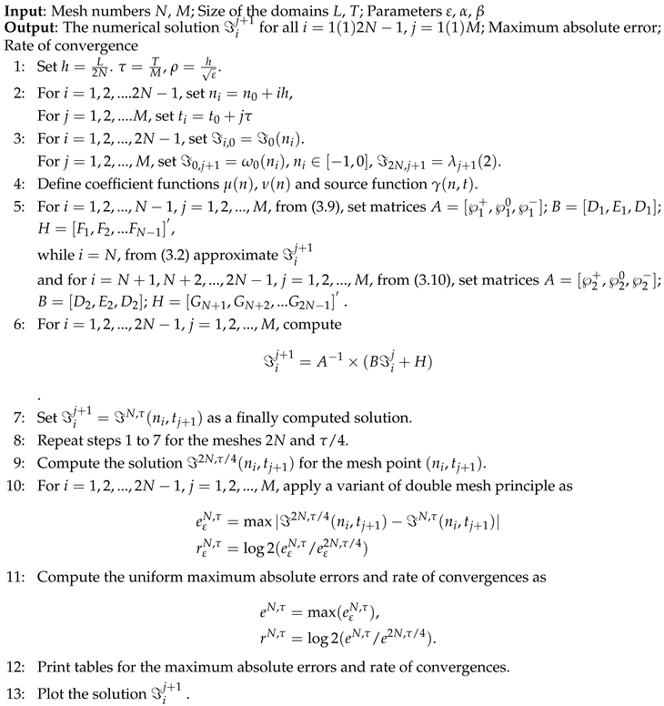
From (3.9) and (3.10), we have system of equations which can be solved using suitable solvers following the computational algorithm given below.

Algorithm 1:

Discrete stability and convergence analyses

Lemma 3.2.

Let

φ_{i}^{j + 1}

is a mesh function which satisfies

φ_{0}^{j + 1} \geq 0

φ_{2 N}^{j + 1} \geq 0

and

L_{ε}^{N . M} φ_{i}^{j + 1} \geq 0

i = 1 (1) 2 N - 1

. Then,

φ_{i}^{j + 1} \geq 0

i = 0 (1) 2 N

Proof.

We refer Lemma 3.6 of [15]. □

Lemma 3.3.

The stability of the solution

ℑ_{i}^{j + 1}

i = 0, 1, . . ., 2 N

of (3.8) is estimated as

| ℑ_{i}^{j + 1} | \leq β^{- 1} ∥ L_{ε}^{N, M} ℑ ∥ + max {| ω^{j + 1} (0) |, | λ^{j + 1} (2) |} .

Proof.

Consider barrier functions

ϖ_{i, \pm}^{j + 1}

given by

ϖ_{i, \pm}^{j + 1} = \frac{1}{β} ∥ L_{ε}^{N, M} ℑ ∥ + sup {| ω^{j + 1} (0) |, | λ^{j + 1} (2) |} \pm ℑ_{i}^{j + 1} .

For

i = 0

, we have

ϖ_{0, \pm}^{j + 1} \geq 0

and for

i = 2 N

, we have

ϖ_{2 N, \pm}^{j + 1} \geq 0

For

i = 1 (1) N

, by (3.8) we obtain

\begin{matrix} L_{ε, 1}^{j + 1} ϖ_{i, \pm}^{j + 1} = & \frac{- ε Δ t σ_{0}}{h^{2}} [ϖ_{i, \pm}^{j + 1} - 2 ϖ_{i, \pm}^{j + 1} + ϖ_{i, \pm}^{j + 1}] + p_{i + 1} ϖ_{i + 1, \pm}^{j + 1} + p_{i} ϖ_{i, \pm}^{j + 1} + p_{i} ϖ_{i - 1, \pm}^{j + 1} \\ + q_{i + 1} ω_{i + 1 - N} + q_{i} ω_{i - N} + q_{i - 1} ω_{i - 1 - N} \\ = & \pm L_{ε, 1}^{j + 1} ℑ_{i}^{j + 1} + p_{i + 1} [β^{- 1} ∥ L_{ε, 1}^{N, M} ℑ_{i + 1}^{j + 1} ∥ + sup {| ω^{j + 1} (0) |, | λ^{j + 1} (2) |}] \\ + p_{i} [β^{- 1} ∥ L_{ε, 1}^{N, M} ℑ_{i}^{j + 1} ∥ + sup {| ω^{j + 1} (0) |, | λ^{j + 1} (2) |}] \\ + p_{i - 1} [β^{- 1} ∥ L_{ε, 1}^{N, M} ℑ_{i - 1}^{j + 1} ∥ + sup {| ω^{j + 1} (0) |, | λ^{j + 1} (2) |}] \\ \geq & (P_{i + 1} + p_{i} + p_{i - 1}) sup {| ω^{j + 1} (0) |, | λ^{j + 1} (2) |} \geq 0 . \end{matrix}

Similarly, for

i = 1 (1) N

, one can obtain

\begin{matrix} L_{ε, 2}^{j + 1} ϖ_{i, \pm}^{j + 1} = & \frac{- ε Δ t σ_{2}}{h^{2}} [ϖ_{i, \pm}^{j + 1} - 2 ϖ_{i, \pm}^{j + 1} + ϖ_{i, \pm}^{j + 1}] + p_{i + 1} ϖ_{i + 1, \pm}^{j + 1} + p_{i} ϖ_{i, \pm}^{j + 1} + p_{i} ϖ_{i - 1, \pm}^{j + 1} \\ + q_{i + 1} ℑ_{i + 1 - N}^{j + 1} + q_{i} ℑ_{i - N}^{j + 1} + q_{i - 1} ℑ_{i - 1 - N}^{j + 1} \\ = & \pm L_{ε, 1}^{j + 1} ℑ_{i}^{j + 1} + p_{i + 1} [β^{- 1} ∥ L_{ε, 1}^{N, M} ℑ_{i + 1}^{j + 1} ∥ + sup {| ω^{j + 1} (0) |, | λ^{j + 1} (2) |}] \\ + p_{i} [β^{- 1} ∥ L_{ε, 1}^{N, M} ℑ_{i}^{j + 1} ∥ + sup {| ω^{j + 1} (0) |, | λ^{j + 1} (2) |}] \\ + p_{i - 1} [β^{- 1} ∥ L_{ε, 1}^{N, M} ℑ_{i - 1}^{j + 1} ∥ + sup {| ω^{j + 1} (0) |, | λ^{j + 1} (2) |}] \\ + q_{i + 1} [β^{- 1} ∥ L_{ε, 1}^{N, M} ℑ_{i + 1 - N}^{j + 1} ∥ + sup {| ω^{j + 1} (0) |, | λ^{j + 1} (2) |}] \\ + q_{i} [β^{- 1} ∥ L_{ε, 1}^{N, M} ℑ_{i - N}^{j + 1} ∥ + sup {| ω^{j + 1} (0) |, | λ^{j + 1} (2) |}] \\ + q_{i - 1} [β^{- 1} ∥ L_{ε, 1}^{N, M} ℑ_{i - 1 - N}^{j + 1} ∥ + sup {| ω^{j + 1} (0) |, | λ^{j + 1} (2) |}] \\ \geq & β sup {| ω^{j + 1} (0) |, | λ^{j + 1} (2) |} \geq 0 . \end{matrix}

Applying Lemma 3.1, the stability estimate holds true. □

Theorem 3.1.

Let

ℑ^{j + 1} (n_{i})

and

ℑ_{i}^{j + 1}

are the solutions of (3.1) and (3.8), respectively. Then, the point-wise error in the spatial direction is bounded as

| ℑ^{j + 1} (n_{i}) - ℑ_{i}^{j + 1} | \leq C N^{- 2}, i = 1, 2, . . ., 2 N .

for constant C independent of ε and N.

Proof.

By local truncation error of finite difference methods [16], we have

\begin{matrix} | L_{ε}^{N, M} (ℑ^{j + 1} (n_{i}) - ℑ_{i}^{j + 1}) | = & | L_{ε}^{M} ℑ^{j + 1} (n_{i}) - L_{ε}^{N, M} ℑ_{i}^{j + 1} | \\ = & | - c_{ε} ℑ_{n n}^{j + 1} (n_{i}) + \frac{c_{ε} σ}{h^{2}} [ℑ_{i + 1}^{j + 1} - 2 ℑ_{i}^{j + 1} + ℑ_{i - 1}^{j + 1}] | . \end{matrix}

(3.11)

Taylor’s series expansion on

ℑ_{i - 1}^{j + 1}

and

ℑ_{i + 1}^{j + 1}

gives

\begin{matrix} ℑ_{i + 1}^{j + 1} = ℑ_{i}^{j + 1} + h ℑ_{n}^{j + 1} + \frac{h^{2}}{2!} ℑ_{n n}^{j + 1} + \frac{h^{3}}{3!} ℑ_{n n n}^{j + 1} + O (h^{4}), \end{matrix}

(3.12)

\begin{matrix} a n d & ℑ_{i - 1}^{j + 1} = ℑ_{i}^{j + 1} - h ℑ_{n}^{j + 1} + \frac{h^{2}}{2!} ℑ_{n n}^{j + 1} - \frac{h^{3}}{3!} ℑ_{n n n}^{j + 1} + O (h^{4}) . \end{matrix}

(3.13)

Plugging (3.12) and (3.13) into (3.11), we obtain

\begin{matrix} | L_{ε}^{N, M} (ℑ^{j + 1} (n_{i}) - ℑ_{i}^{j + 1}) | = & | - ε Δ t ℑ_{n n}^{j + 1} + ε Δ t σ [ℑ_{n n}^{j = 1} + \frac{2 h^{2}}{4!} ℑ_{n n n n}^{j + 1} + O (h^{4})] \\ \leq & C | ε σ - ε | ∥ ℑ_{n n}^{j + 1} (ξ_{i}) ∥ + C ε σ h^{2} ∥ ℑ_{n n n n}^{j + 1} (ξ_{i}) ∥, ξ_{i} \in [n_{i - 1}, n_{i + 1}] . \end{matrix}

As estimated in [17], we have

| ε σ - ε | \leq C h^{2}

and hence for sufficiently small h, we get

| L_{ε}^{N, M} (ℑ^{j + 1} (n_{i}) - ℑ_{i}^{j + 1}) | \leq C N^{- 2} .

Hence, applying Lemma 3.1 gives the required estimate. □

Theorem 3.2.

Let

ℑ (n, t)

and

ℑ_{i}^{J + 1}

are the solutions of (2.1) and 3.8, respectively. Then, the uniform error estimation is given by

∥ ℑ (n_{i}, t_{j + 1}) - ℑ_{i}^{j + 1} ∥ \leq C (τ + N^{- 2}) .

Proof.

By the triangular inequality, we have

∥ ℑ (n_{i}, t_{j + 1}) - ℑ_{i}^{j + 1} ∥ \leq ∥ ℑ (n_{i}, t_{j + 1}) - ℑ_{i}^{j + 1} ∥ + ∥ ℑ^{j + 1} (n_{i}) - ℑ_{i}^{j + 1} ∥

(3.14)

Using Lemma 3.1 and Theorem 3.1 into (3.14), yields required the uniform error estimate. □

4. Numerical experiments and discussions

In this section, to validate the developed numerical numerical techniques, we solved model examples. As it is tedious to compute the exact solutions of the examples, we apply a variant of the double mesh principle [16,18] as given in Algorithm 1.

Example 4.1.

[9,10]. Consider a SP-PDE given by

ℑ_{t} (n, t) - ε ℑ_{n n} (n, t) + 3 ℑ (n, t) - ℑ (n - 1, t) = 1

ℑ (n, 0) = 0

n \in [0, 2]

ℑ (n, t) = 0

(n, t) \in {(n, t) : - 1 \leq n \leq 0, 0 \leq t \leq 2}

and

ℑ (2, t) = 0

(2, t) \in {(2, t) : t \in [0, 2]}

Example 4.2.

[10]. Consider a SP-PDE given by

ℑ_{t} (n, t) - ε ℑ_{n n} (n, t) + (n + 6) ℑ (n, t) - (n^{2} + 1) ℑ (n - 1, t) = 3

ℑ (n, 0) = 0

n \in [0, 2]

ℑ (n, t) = 0

(n, t) \in {(n, t) : - 1 \leq n \leq 0, 0 \leq t \leq 2}

and

ℑ (2, t) = 0

(2, t) \in {(2, t) : t \in [0, 2]}

Example 4.3.

[9]. Consider a SP-PDE given by

ℑ_{t} (n, t) - ε ℑ_{n n} (n, t) + 5 ℑ (n, t) - 2 ℑ (n - 1, t) = - 2

ℑ (n, 0) = sin (π n)

n \in [0, 2]

ℑ (n, t) = 0

(n, t) \in {(n, t) : - 1 \leq n \leq 0, 0 \leq t \leq 2}

and

ℑ (2, t) = 0

(2, t) \in {(2, t) : t \in [0, 2]}

The examples are treated applying the developed numerical algorithm on a Matlab software package. We computed the maximum absolute errors (MAEs) and convergences rates (CRs) to validate the method and the numerical solutions are simulated graphically for each example. In Table 1, Table 2 and Table 3, the MAEs and CRs are shown for each examples respectively. From the tables, one can see that reducing the number of meshes reduces the error and reducing

ε

yields stabled Maximum point-wise errors, which indicate that the technique is uniformly convergent. Table 4 shows comparisons of the present result with other published results.

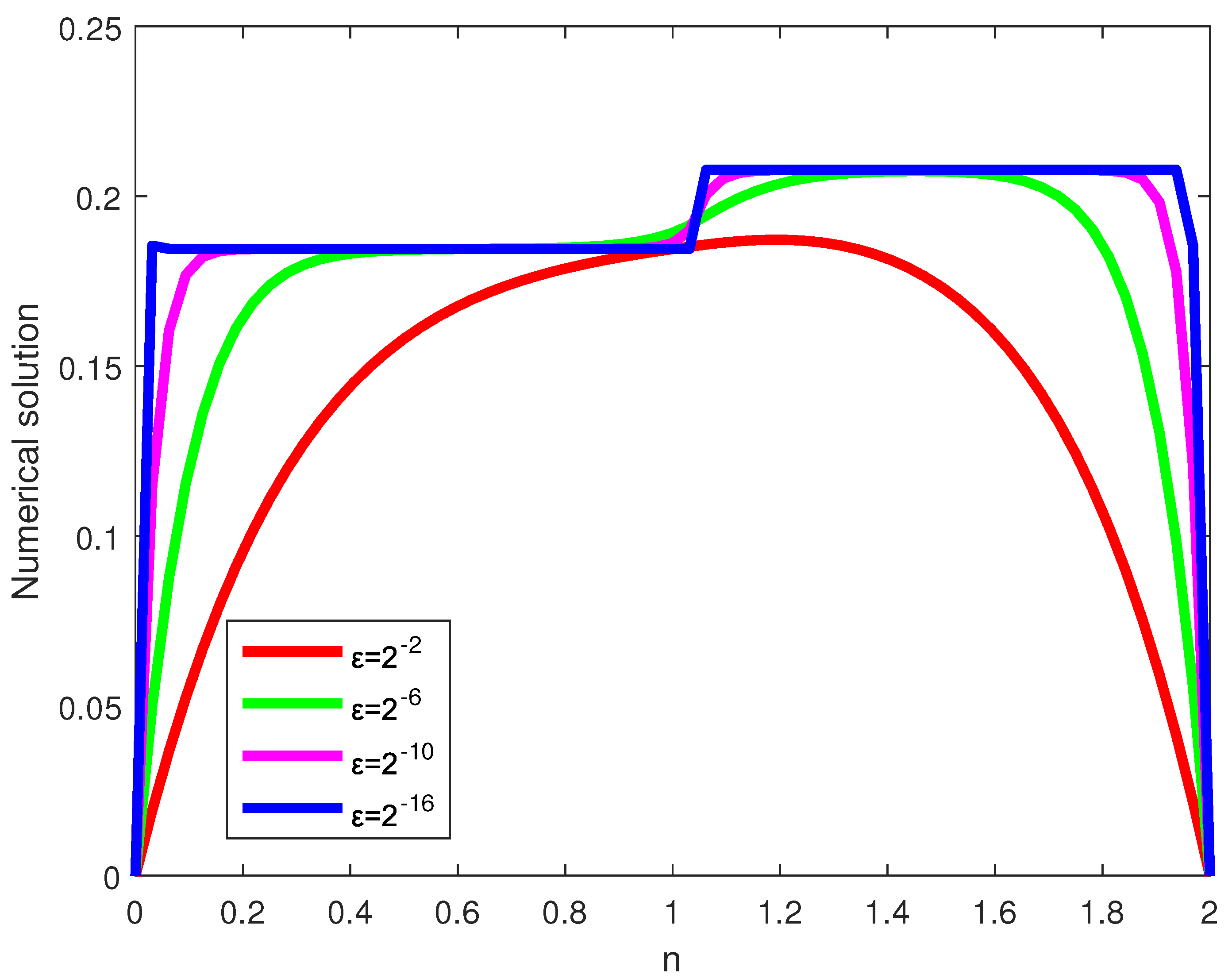
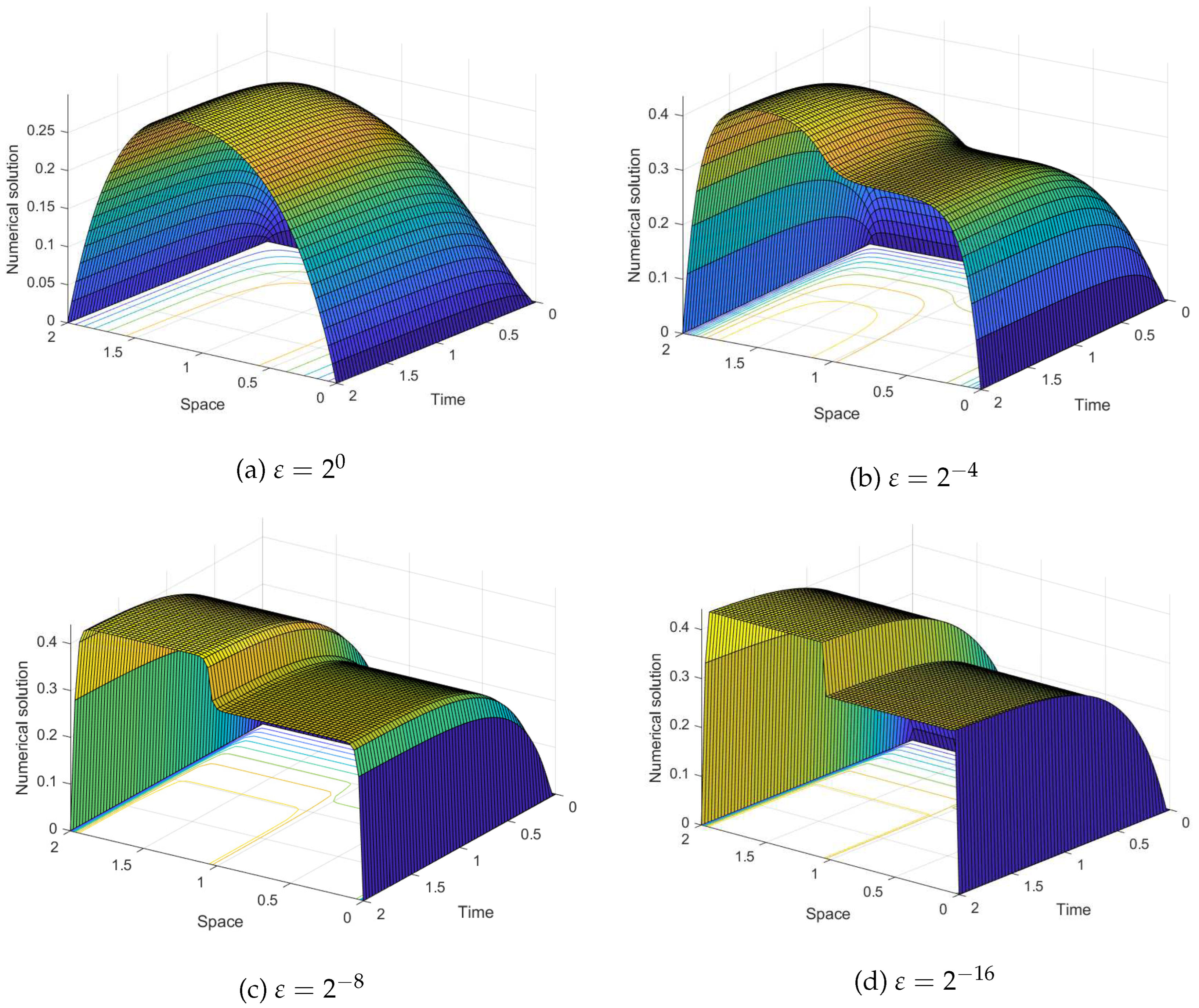
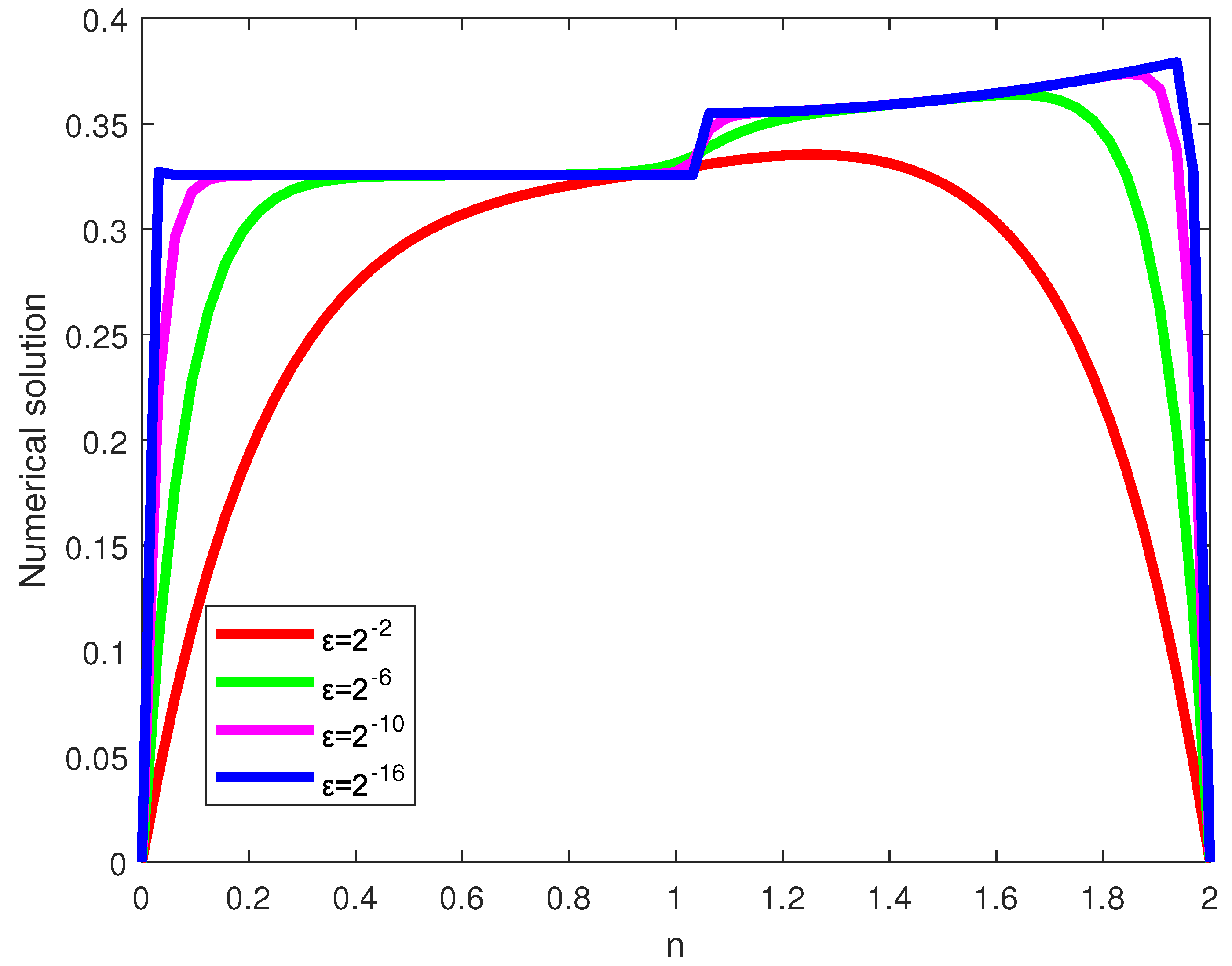
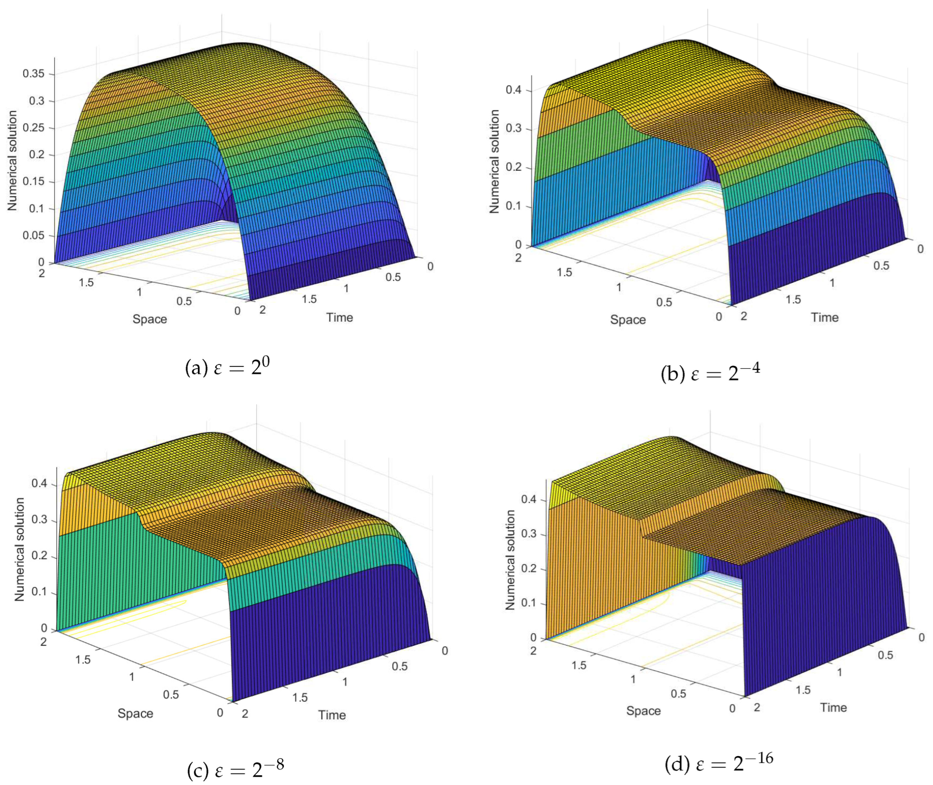
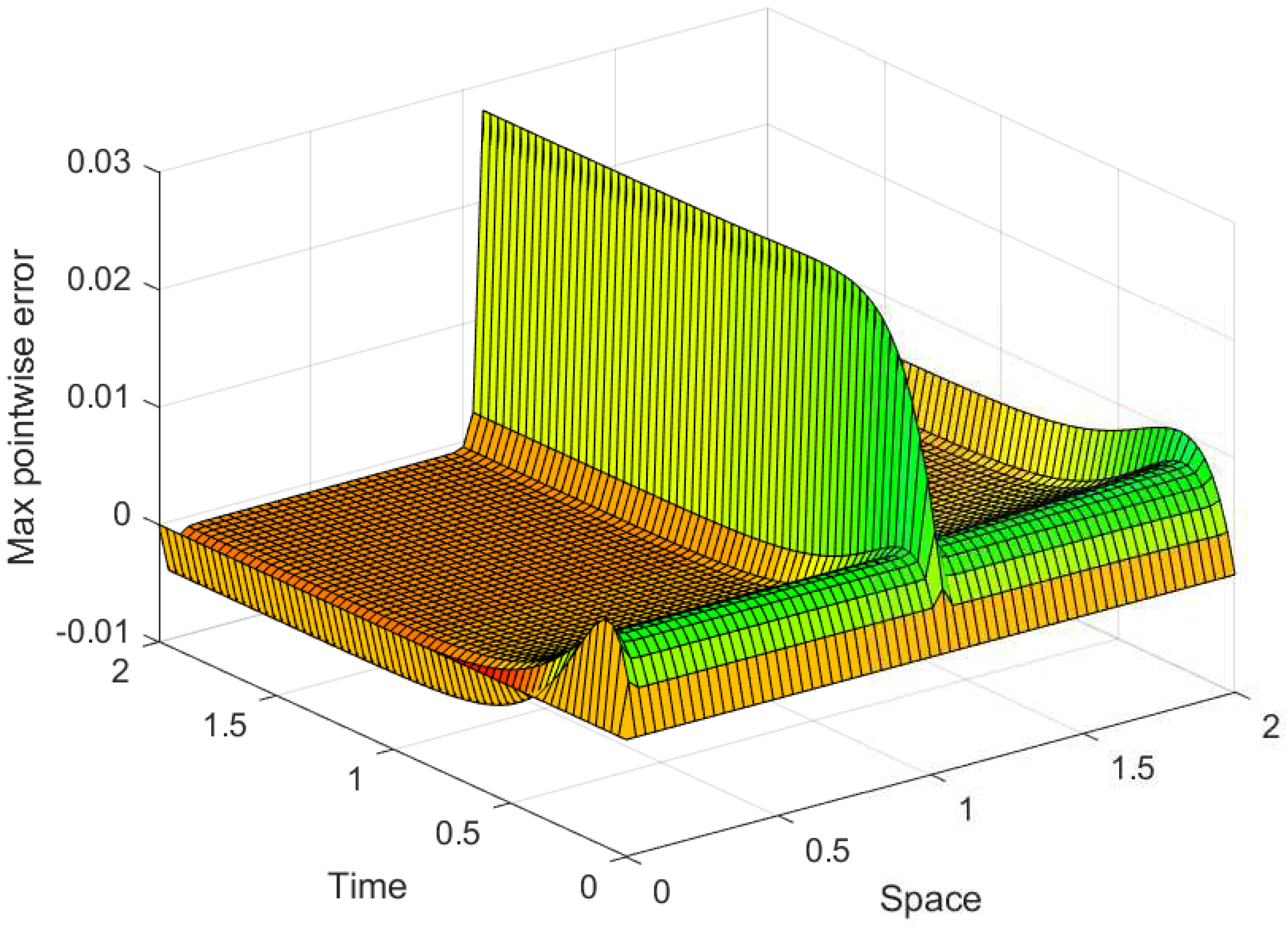
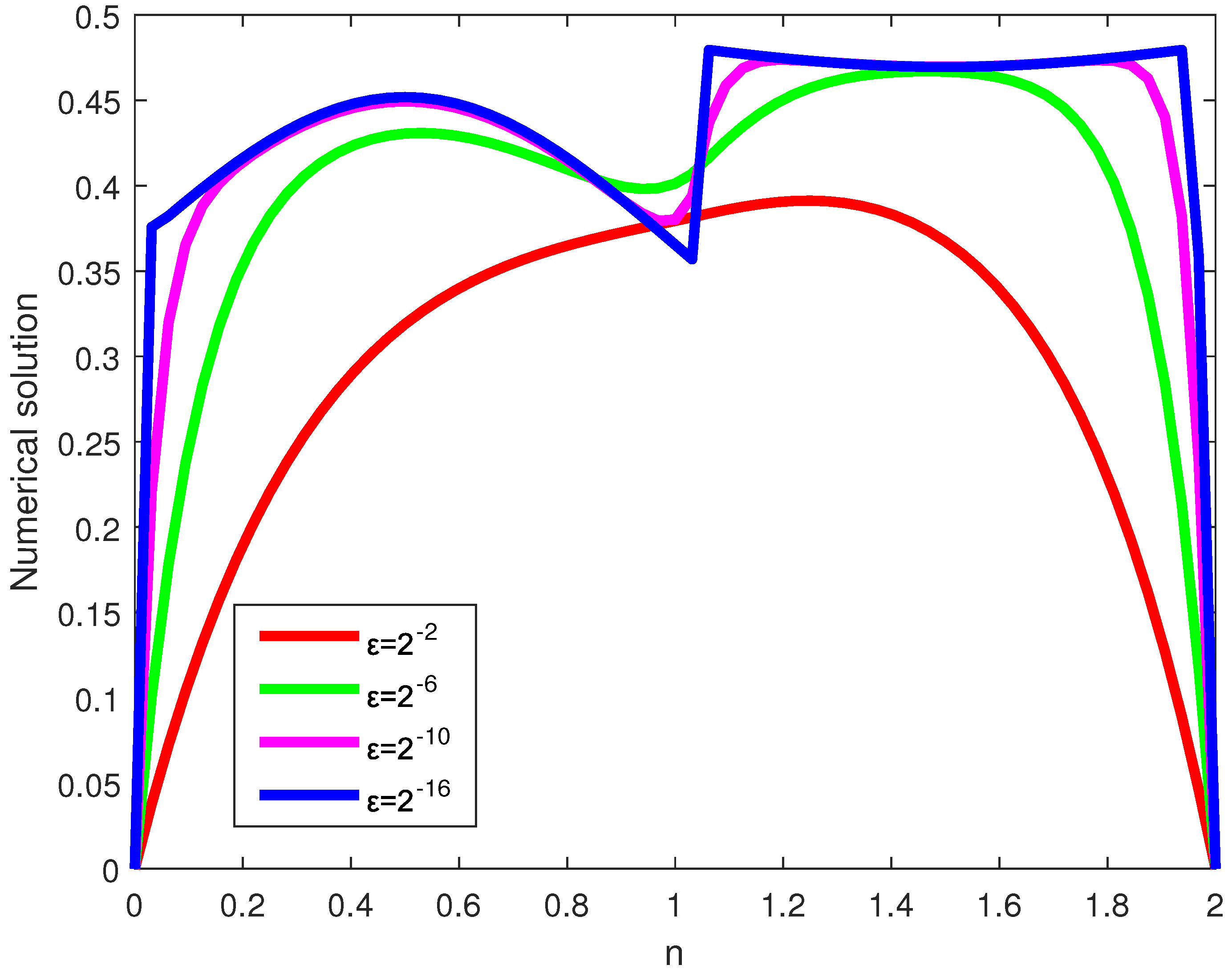
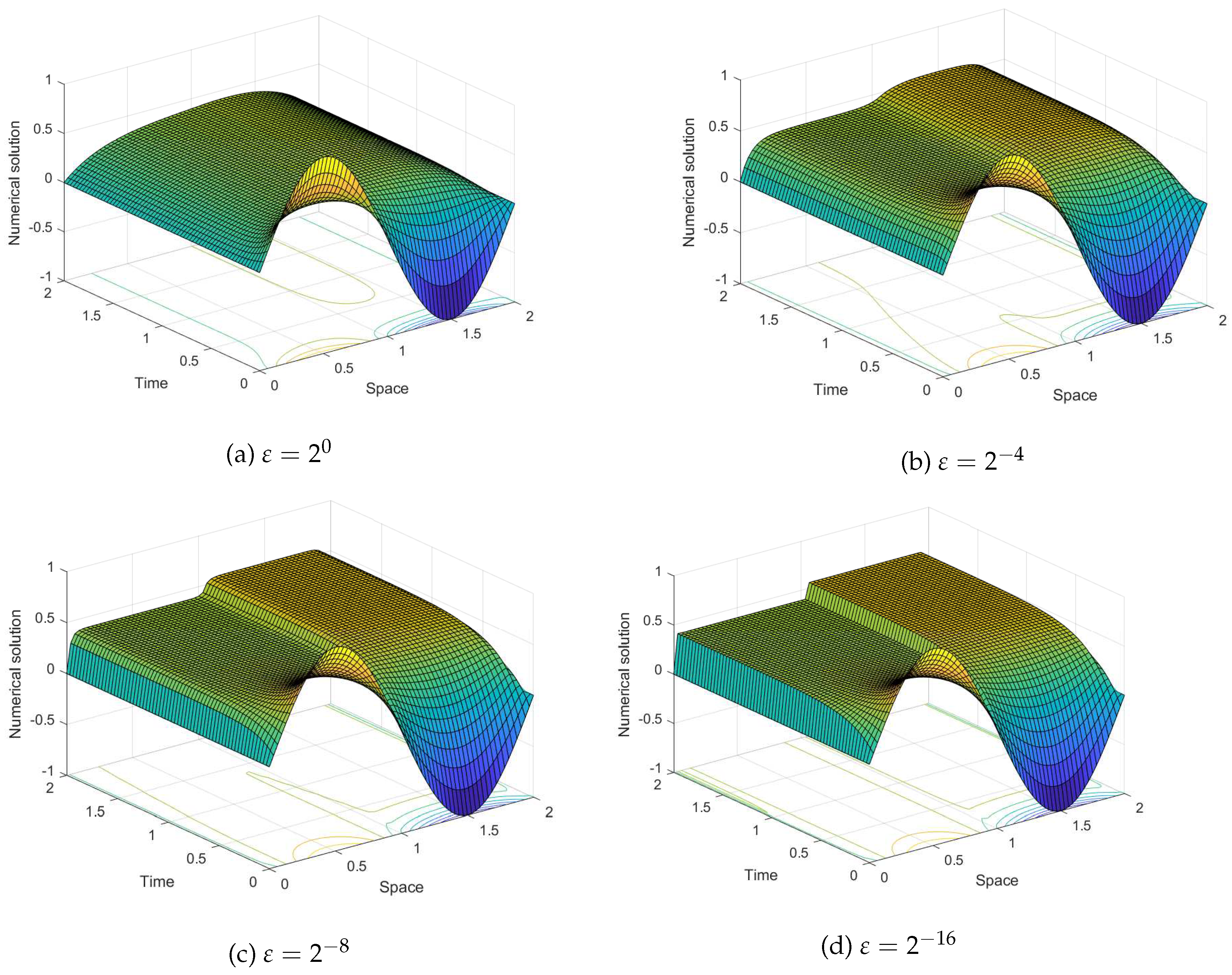
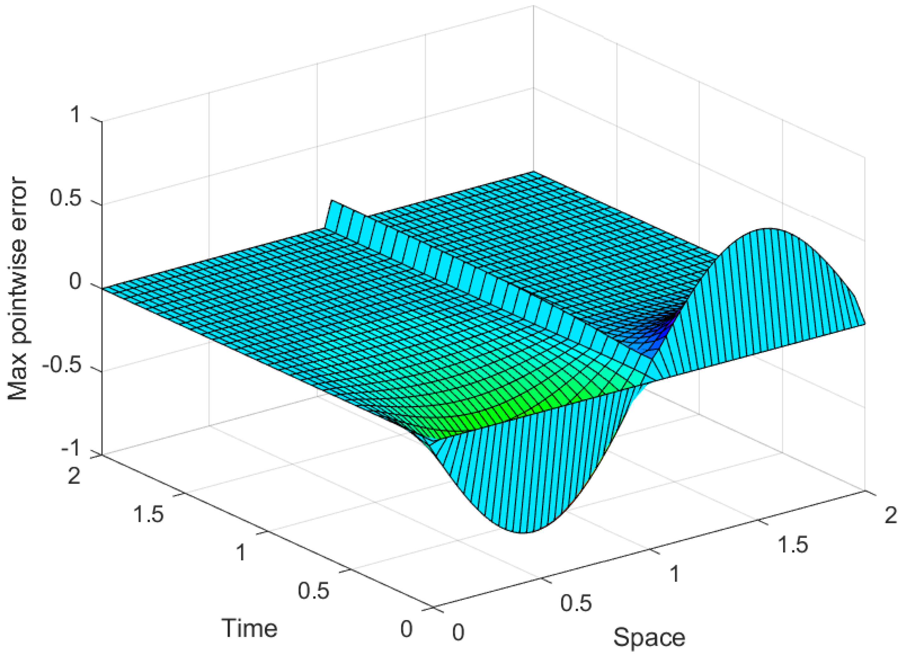
Simulations of the numerical solutions and error profiles are displayed graphically for each examples. In the line plots given in Figure 1, Figure 4 and Figure 7, the effect of

ε

on the solution profile are shown for Examples 4.1, 4.2 and 4.3, respectively. The influence of

ε

is also simulated in the surface plots given in Figure 2, Figure 5 and Figure 8 for each examples. From such figures, one can visualize that reducing the value of

ε

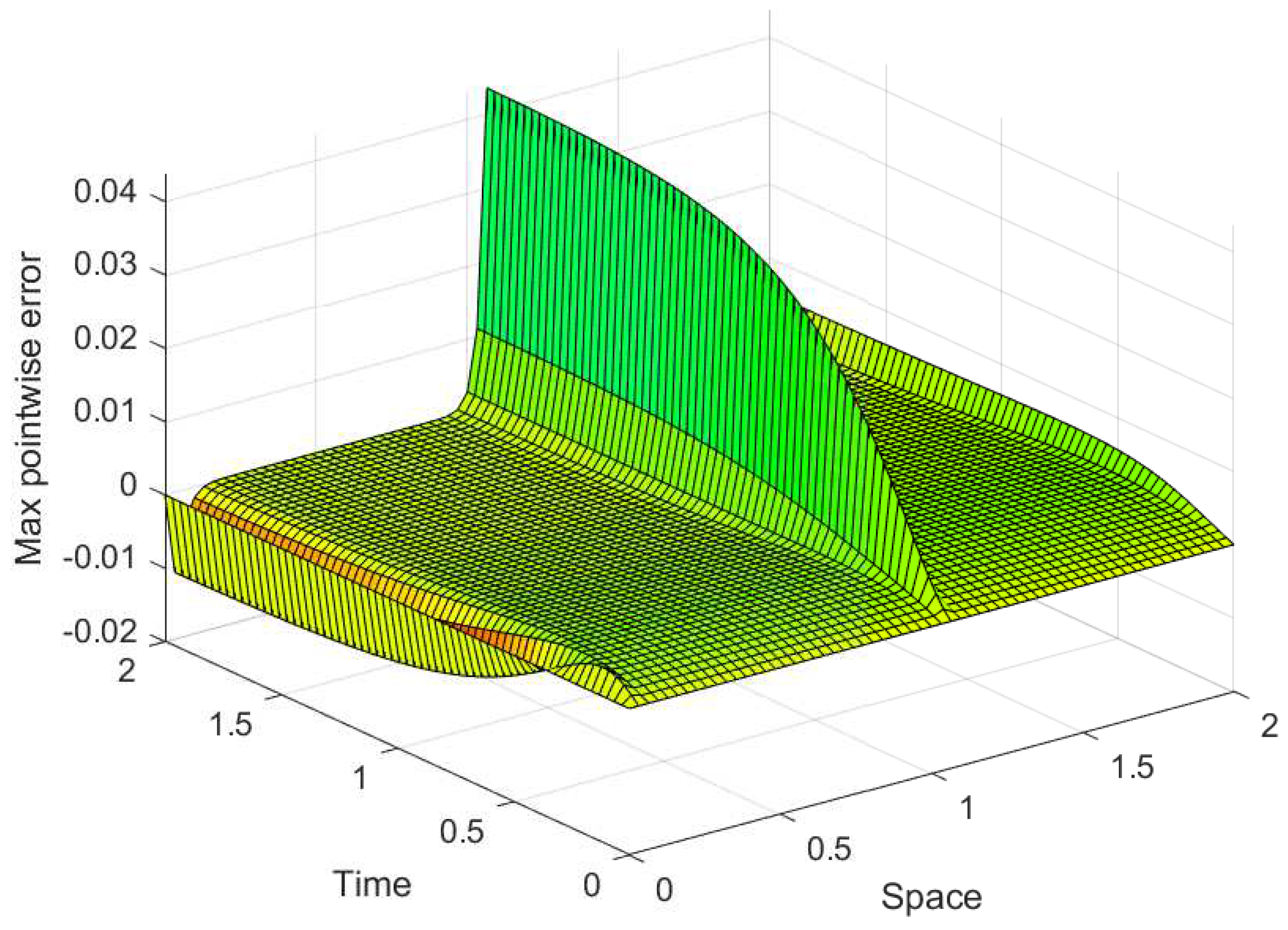
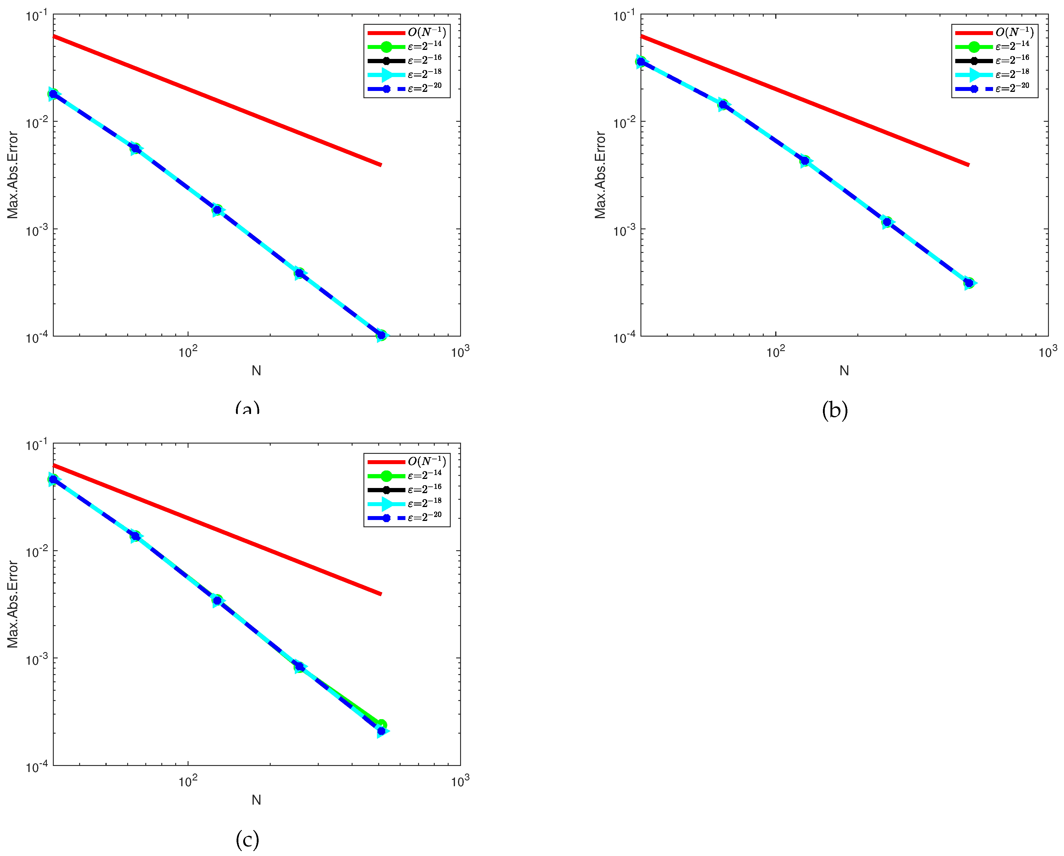
reduces the width of the layer regions yielding more steep gradients. From the maximum error profiles given in Figure 3, Figure 6 and Figure 9, one can observe that maximum error is committed in the interior layers raised due to the large negative shift. Figure 10 is log-log plots of the MAEs versus N for the examples, confirming the convergence of the scheme uniformly.

5. Conclusion

In this article, a numerical method is formulated and its computational algorithm is provided to solve singularly perturbed parabolic partial differential equations involving a negative shift. The influence of

ε

causes boundary layers and the negative shift term causes interior layer in the solutions. We treated the continuous problem by transformed it into a finite difference method applying implicit Euler technique in time variable and using an exponentially fitted tension spline function on a uniform grids in space variable. The stability and convergence analyses of the formulated method are investigated and proved. The step-wise computational algorithm is also provided, and to test the formulated technique, numerical experiments are carried out. For the considered examples, the numerical solutions and the effect of

ε

and the large negative shift on the solution profile are simulated graphically. MAEs and CRs of the numerical solutions are computed for each example. From the uniform convergence analysis and numerical experiments, we conclude that the formulated technique convergent uniformly with order one in time and second order in the spatial direction.

Author Contributions

Conceptualization, GF. D; methodology, AH. E; software, AH. E; validation, AH. E and GF. D; formal analysis, AH. E; investigation, AH. E and GF. D; writing-original draft preparation, AH. E; supervision, GF. D. Both authors have agreed on the submitted version of the manuscript.

Funding

This research received no external funding.

Informed Consent Statement

Not applicable.

Data Availability Statement

In this research work, there is no data used to support our findings.

Acknowledgments

The authors would like to express sincere gratitude to the editor in chief for his expertise handling of the submitted manuscript. We also grateful to the anonymous reviewers for their thoughtful and thorough review of the manuscript. We would like to extend our appreciation to our colleagues, mentors and friends who have provided valuable insights and encouragement throughout this research endeavor.

Conflicts of Interest

The authors declare no conflict of interest.

References

Gu, Keqin and Chen, Jie and Kharitonov, Vladimir L. Stability of time-delay systems. Springer Science & Business Media, 2003.
K. Apratim and O.S. Otugen. Modeling the arterial circulation: A review of recent developments and future directions. Journal of Biomechanical Engineering 2011, 133(9).
M. Di Bernardo, C. J. Budd, and A.R. Champneys. Bifurcation and stability of delayed systems, International Series of Numerical Mathematics, 2008; 152.
D.A. Hoyle and M.J. Chappell. Steady-state solutions for two-species reaction-diffusion delays systems: Applications to chemically reacting flow. Journal of Mathematical Chemistry 2005, 34(4).
S. Mondal. Stabilization of fluid flow with distributed time delays using a variable structure controller. Journal of Process Control 2017, 49.
Meyer-Bäse, Anke and Ohl, Frank and Scheich, Henning. Singular perturbation analysis of competitive neural networks with different time scales. Neural Computation 1996, 8(8), 1731–1742. [CrossRef]
Kumar, Devendra and Kumari, Parvin. A parameter-uniform scheme for singularly perturbed partial differential equations with a time lag. Numerical Methods for Partial Differential Equations 2020, 36(4), 868–886. [CrossRef]
Duressa, Gemechis File and Woldaregay, Mesfin Mekuria. Fitted numerical scheme for solving singularly perturbed parabolic delay partial differential equations. Tamkang Journal of Mathematics 2022, 52(4), 345–362. [CrossRef]
Bansal, Komal and Sharma, Kapil K. Parameter-robust numerical scheme for time-dependent singularly perturbed reaction–diffusion problem with large delay. Numerical Functional Analysis and Optimization 2018, 39, 127–154. 127–154. [CrossRef]
Kumar, Devendra and Kumari, Parvin. Parameter-uniform numerical treatment of singularly perturbed initial-boundary value problems with large delay. Applied Numerical Mathematics 2020, 153, 412–429. [CrossRef]
Swaminathan, Parthiban and Sigamani, Valarmathi and Victor, Franklin. Numerical Method for a Singularly Perturbed Boundary Value Problem for a Linear Parabolic Second Order Delay Differential Equation. Differential Equations and Numerical Analysis 2016, 117–133. [CrossRef]
Sharma, Nitika and Kaushik, Aditya. A uniformly convergent difference method for singularly perturbed parabolic partial differential equations with large delay and integral boundary condition. Journal of Applied Mathematics and Computing 2023, 89(1), 1071–1093. [CrossRef]
Andargie Tiruneh, Awoke and Adamu Derese, Getachew and Amsalu Ayele, Mulunesh. Singularly perturbed reaction diffusion problem with large spatial delay via non-standard fitted operator method. Research in Mathematics 2023, 10(1), pp. 2171698. [CrossRef]
Ejere, Ababi Hailu and Duressa, Gemechis File and Woldaregay, Mesfin Mekuria and Dinka, Tekle Gemechu. A Parameter-Uniform Numerical Scheme for Solving Singularly Perturbed Parabolic Reaction-Diffusion Problems with Delay in the Spatial Variable. International Journal of Mathematics and Mathematical Sciences 2023, 2023. [CrossRef]
Ejere, Ababi Hailu and Duressa, Gemechis File and Woldaregay, Mesfin Mekuria and Dinka, Tekle Gemechu. A tension spline fitted numerical scheme for singularly perturbed reaction-diffusion problem with negative shift. BMC Research Notes 2023, 16(1), 1–16. [CrossRef]
Munyakazi, Justin B and Patidar, Kailash C. A fitted numerical method for singularly perturbed parabolic reaction-diffusion problems. Computational and applied mathematics 2013, 13, 509–519. [CrossRef]
Doolan, Edward P and Miller, John JH and Schilders, Willy HA. Uniform numerical methods for problems with initial and boundary layers. Boole Press, 1980.
Wondimu, Getu Mekonnen and Woldaregay, Mesfin Mekuria and Dinka, Tekle Gemechu and Duressa, Gemechis File. Numerical treatment of singularly perturbed parabolic partial differential equations with nonlocal boundary condition. Frontiers in Applied Mathematics and Statistics 2022, 8, pp.=1005330. [CrossRef]

Short Biography of Authors

Ababi Hailu Ejere received his Ph.D in Mathematics from Adama Science and Technology University. Currently, he is working at Ethiopian Defence University as a lecturer and researcher. His research interest spans in the areas of Numerical analysis and computing, Singular perturbation problems and refinement of system of equations. He contributed research articles to various international reputable journals.

Gemechis File Duressa received his Ph.D in Mathematics from National Institute of Technology Warangal, India. Currently, he is a full Professor of Mathematics at Jimma University. His research interests span on the areas of numerical solutions of differential equations, mainly on singularly perturbed ordinary and partial differential equations. He made numerous contributions in serving as a lecturer, researcher, reviewer, assistant editor and editor for various national and international Journals.

Figure 1. Line plot simulations showing the effect of

ε

on the solutions of Example 4.1.

Figure 1. Line plot simulations showing the effect of

ε

on the solutions of Example 4.1.

Figure 2. Surface plot simulations of the numerical solution of Example 4.1 with

N = 2^{7}

τ = 4^{- 3}

and various value of

ε

Figure 2. Surface plot simulations of the numerical solution of Example 4.1 with

N = 2^{7}

τ = 4^{- 3}

and various value of

ε

Figure 3. Maximum point-wise error profile of Example 4.1 for

ε = 2^{- 8}

Figure 3. Maximum point-wise error profile of Example 4.1 for

ε = 2^{- 8}

Figure 4. Line plot simulations showing the effect of

ε

on the solutions of Example 4.2.

Figure 4. Line plot simulations showing the effect of

ε

on the solutions of Example 4.2.

Figure 5. Surface plot simulations of the numerical solution of Example 4.2 for

N = 2^{7}

τ = 4^{- 3}

and different value of

ε

Figure 5. Surface plot simulations of the numerical solution of Example 4.2 for

N = 2^{7}

τ = 4^{- 3}

and different value of

ε

Figure 6. Maximum point-wise error profile of Example 4.2 for

ε = 2^{- 8}

Figure 6. Maximum point-wise error profile of Example 4.2 for

ε = 2^{- 8}

Figure 7. Line plot simulations showing the effect of

ε

on the solutions of Example 4.3.

Figure 7. Line plot simulations showing the effect of

ε

on the solutions of Example 4.3.

Figure 8. Surface plot simulations of the numerical solution of Example 4.3 for

N = 2^{7}

τ = 4^{- 3}

and different values of

ε

Figure 8. Surface plot simulations of the numerical solution of Example 4.3 for

N = 2^{7}

τ = 4^{- 3}

and different values of

ε

Figure 9. Maximum point-wise error profile of Example 4.3.

Figure 10. Log-log plots of MAEs versus N for the solutions of Example 4.1 in (a), Example 4.2 in (b) and Example 4.3 in (c).

Table 1. MAEs and CRs of Example 4.1 for various

ε

and mesh numbers.

Table 1. MAEs and CRs of Example 4.1 for various

ε

and mesh numbers.

$ε$	$N :$ $2^{5}$	$2^{6}$	$2^{7}$	$2^{8}$	$2^{9}$
↓	$τ :$ $4^{- 1}$	$4^{- 2}$	$4^{- 3}$	$4^{- 4}$	$4^{- 5}$
$2^{- 2}$	1.1736e-02	2.4926e-03	5.5509e-04	1.3443e-04	3.3300e-05
$2^{- 4}$	1.9466e-02	5.1190e-03	1.1780e-03	1.9606e-04	4.7786e-05
$2^{- 6}$	2.3727e-02	5.1915e-03	1.1686e-03	3.6556e-04	7.3489e-05
$2^{- 8}$	2.0057e-02	5.0573e-03	1.6892e-03	3.8786e-04	1.0097e-04
$2^{- 10}$	1.8114e-02	6.6013e-03	1.5188e-03	3.7730e-04	1.0112e-04
$2^{- 12}$	1.7980e-02	5.6213e-03	1.5625e-03	3.4160e-04	1.0220e-04
$2^{- 14}$	1.7979e-02	5.6103e-03	1.5006e-03	3.8644e-04	1.0184e-04
$2^{- 16}$	1.7979e-02	5.6103e-03	1.5006e-03	3.8636e-04	1.0184e-04
$2^{- 18}$	1.7979e-02	5.6103e-03	1.5006e-03	3.8636e-04	1.0184e-04
$2^{- 20}$	1.7979e-02	5.6103e-03	1.5006e-03	3.8636e-04	1.0184e-04
$e^{N, τ}$	2.3727e-02	6.6013e-03	1.6892e-03	3.8644e-04	1.0220e-04
$r^{N, τ}$	1.8457	1.9664	2.1280	1.9188	-
CPU (s)	0.0613	0.2344	1.6094	41.0160	89.7541

Table 2. MAEs and CRs of Example 4.2 for various

ε

and mesh numbers.

Table 2. MAEs and CRs of Example 4.2 for various

ε

and mesh numbers.

$ε$	$N :$ $2^{5}$	$2^{6}$	$2^{7}$	$2^{8}$	$2^{9}$
↓	$τ :$ $4^{- 1}$	$4^{- 2}$	$4^{- 3}$	$4^{- 4}$	$4^{- 5}$
$2^{- 2}$	2.7596-02	8.2814e-03	17841e-03	4.1167e-04	1.0052e-04
$2^{- 4}$	3.8536e-02	1.3953e-02	3.0303e-03	6.1916e-04	1.4540e-04
$2^{- 6}$	3.9507e-02	1.3834e-02	3.2716e-03	8.2355e-04	2.1448e-04
$2^{- 8}$	3.6724e-02	1.3995e-02	3.9298e-03	1.2099e-03	2.5171e-04
$2^{- 10}$	3.6069e-02	1.4599e-02	3.4739e-03	1.4635e-03	2.9312e-04
$2^{- 12}$	3.6042e-02	1.4374e-02	4.3050e-03	1.2310e-03	3.0513e-04
$2^{- 14}$	3.6042e-02	1.4372e-02	4.2906e-03	1.1563e-03	3.1248e-04
$2^{- 16}$	3.6042e-02	1.4372e-02	4.2906e-03	1.1562e-03	3.1237e-04
$2^{- 18}$	3.6042e-02	1.4372e-02	4.2906e-03	1.1562e-03	3.1237e-04
$2^{- 20}$	3.6042e-02	1.4372e-02	4.2906e-03	1.1562e-03	3.1237e-04
$e^{N, τ}$	3.9507e-02	1.4599e-02	4.3050e-03	1.2311e-03	3.1248e-04
$r^{N, τ}$	1.4362	1.7618	1.8061	1.9781	-
CPU (s)	0.07813	0.3281	3.7813	58.0161	94.3152

Table 3. MAEs and CRs of Example 4.1 for various

ε

and mesh numbers.

Table 3. MAEs and CRs of Example 4.1 for various

ε

and mesh numbers.

$ε$	$N :$ $2^{5}$	$2^{6}$	$2^{7}$	$2^{8}$	$2^{9}$
↓	$τ :$ $4^{- 1}$	$4^{- 2}$	$4^{- 3}$	$4^{- 4}$	$4^{- 5}$
$2^{- 2}$	3.1077e-02	6.5142e-03	1.0213e-03	1.6546e-04	3.9589e-05
$2^{- 4}$	4.1719e-02	9.3243e-03	1.6287e-03	2.8643e-04	6.7554e-05
$2^{- 6}$	5.2176e-02	1.4938e-02	3.3470e-03	3.5643e-04	7.6210e-05
$2^{- 8}$	5.2354e-02	1.1457e-02	3.6393e-03	3.8061e-04	9.1247e-05
$2^{- 10}$	4.7519e-02	1.0446e-02	3.3255e-03	3.6856e-04	8.7615e-05
$2^{- 12}$	4.6085e-02	1.4401e-02	3.8045e-03	9.4499e-04	2.1712e-04
$2^{- 14}$	4.6012e-02	1.3660e-02	3.4654e-03	8.1789e-04	2.3763e-04
$2^{- 16}$	4.6011e-02	1.3654e-02	3.4162e-03	8.3367e-04	2.0961e-04
$2^{- 18}$	4.6011e-02	1.3654e-02	3.4162e-03	8.3359e-04	2.0956e-04
$2^{- 20}$	4.6011e-02	1.3654e-02	3.4162e-03	8.3359e-04	2.0956e-04
$e^{N, τ}$	5.2354e-02	1.4401e-02	3.8045e-03	9.4499e-04	2.3763e-04
$r^{N, τ}$	1.8662	1.9204	2.0093	1.9916	-
CPU (s)	0.0234	0.3281	4.6344	48.7970	97.5253

Table 4. Comparison of our method with other published works.

CRs for Example 4.1
	N:	$2^{6}$	$2^{7}$	$2^{8}$	$2^{9}$
	$τ$ :	$4^{- 2}$	$4^{- 3}$	$4^{- 4}$	$4^{- 5}$
present method
	$ε = 2^{- 20}$	1.6802	1.9026	1.9575	1.6722
Results in [9]
	$ε = 2^{- 20}$	1.3369	1.5402	1.6333	1.6261
MAEs and CRs of Example 4.1
	N:	18	36	72	144
	$τ$ :	36	72	144	288
present method
	$e^{N}$	2.6176e-03	1.3380e-03	6.7889e-04	3.4436e-04
	$r^{N}$	0.9682	0.9788	0.9793	0.9824
Results in [10]
	$e^{N, M}$	1.1200e-02	7.0100e-03	2.9700e-03	1.1400e-03
	$r^{N, M}$	0.6760	1.2390	1.3814	1.4895
MAEs and CRs of Example 4.2
Present method
	$e^{N, τ}$	7.3137e-03	3.9025e-03	2.0203e-03	1.0307e-03
	$r^{N, τ}$	0.9062	0.9479	0.9709	0.9727
Results in [10]
	$e^{N, τ}$	1.36e-02	1.09e-02	5.56e-03	2.2800e-03
	$r^{N, τ}$	0.3193	0.9712	1.2861	0.8787
MAEs and CRs for Example 4.3
	N:	$2^{6}$	$2^{7}$	$2^{8}$	$2^{9}$
	$τ$ :	$4^{- 2}$	$4^{- 3}$	$4^{- 4}$	$4^{- 5}$
present method
	$ε = 2^{- 20}$	1.7527	1.9989	2.0350	1.9920
Results in [9]
	$ε = 2^{- 20}$	1.7908	1.8354	1.5091	1.6257

Disclaimer/Publisher’s Note: The statements, opinions and data contained in all publications are solely those of the individual author(s) and contributor(s) and not of MDPI and/or the editor(s). MDPI and/or the editor(s) disclaim responsibility for any injury to people or property resulting from any ideas, methods, instructions or products referred to in the content.

© 2023 by the authors. Licensee MDPI, Basel, Switzerland. This article is an open access article distributed under the terms and conditions of the Creative Commons Attribution (CC BY) license (http://creativecommons.org/licenses/by/4.0/).

Copyright: This open access article is published under a Creative Commons CC BY 4.0 license, which permit the free download, distribution, and reuse, provided that the author and preprint are cited in any reuse.

MDPI Initiatives

Important Links

Choose an area of interest and we will send you notifications of new preprints at your preferred frequency.

Disclaimer

A Fitted Numerical Scheme with Algorithm for Singularly Perturbed Parabolic Partial Differential Equations with Large Negative Shift

Abstract

1. Introduction

2. Preliminaries and a priori estimates

3. Numerical formulation and computational procedures

Discrete stability and convergence analyses

4. Numerical experiments and discussions

5. Conclusion

Author Contributions

Funding

Informed Consent Statement

Data Availability Statement

Acknowledgments

Conflicts of Interest

References

Short Biography of Authors

MDPI Initiatives

Important Links

Subscribe