Preprint
Article

Implementation of Simulation Modeling of Single and High-Volume Machine-Building Productions

Altmetrics

Downloads

141

Views

63

Comments

0

A peer-reviewed article of this preprint also exists.

Submitted:

07 October 2023

Posted:

07 October 2023

Read the latest preprint version here

Alerts
Abstract
The authors of the article analyze the existing methods and models of technological preparation of machine-building industries. The structure of a three-level simulation model with network-centric control, the structures of individual elements of the simulation model and the process of simulation modeling are described. The criteria for choosing a rational option for the processing technological route have been determined. During the research, a simulation program was implemented in C++. It allows you to select the optimal scenario for the operation of a production site based on two criteria: time and cost. The volume of implementation is about 2x10³ lines of code. A diagram of the modeling algorithm for the implemented program, a description of the classes and their interactions are given in the article. The developed simulation model was tested at a machine-building enterprise using the example of the “Pusher” part, manufactured under single-unit production condi-tions. The technological equipment used for the manufacture of this part was formed in the form of input data of the simulation model. The results of simulation modeling for the selected part are described. For each variant of the technological processing route, the values of variable costs and the duration of the production cycle were determined.
Keywords: 
Subject: Engineering  -   Mechanical Engineering

1. Introduction

The current direction of organizing modern production is the transition to advanced digital, intelligent production technologies and robotic systems. Within this direction, the defining trend of the future material production of goods and services is the use of production networks with network-centric control [1]. Examples of modern production sites are complexes of multifunctional computer numerical control (CNC) machines, 3D printers and robots, which are integrated into a network to create conditions for effective planning and optimal implementation of parallel technological processes [2,3,4,5]. A feature of technological processes is their adaptability to small-scale or piece production in such areas as mechanical engineering, processing of raw materials, assembly of multi-component products, etc. [6,7]
Technological preparation of production (hereinafter referred to as TPP) is one of the most important stages of the process for the production of parts. The Chamber of Commerce and Industry provides for solving problems in many areas: for example, ensuring the manufacturability of the product design; design of technological processes and development of technological documentation; design and manufacture of technological equipment; organization and management of the process of technological preparation of production [8]. As a rule, production automation and manufacturing processes come down to the typification of design elements and technological processes [9], although in conditions of single and small-scale production this approach may not be effective due to the high costs of preparatory work [10].
This work is aimed at building a simulation model in order to reduce the duration and labor intensity of technological preparation of single and small-scale production, and increase the efficiency of production processes.
To build a new simulation model, it is necessary to use an analysis of various technological processing routes and the technological equipment used. One of the most effective methods for assessing many options for technological processes and selecting the most suitable one is simulation modeling of production processes and multi-criteria analysis based on a selected set of criteria [11,12]. When speaking about technological preparation of production, the authors will further refer to its model.
One of the factors for increasing the efficiency of an enterprise and its competitiveness is the automation of production processes [13]. Production processes also include technological preparation of production, the automation of which through digitalization ensures not only a reduction in production preparation time, but also optimizes the overall costs of manufacturing products. In addition, such automation ensures and allows you to adapt the technological process to changes in external conditions and quickly recalculate the technological process [14].
The main approaches of modern TPP models include: the theory of computational complexity, analysis of design and technological elements, analysis of the similarity of design solutions, and a scheduling system.
Complexity theory, as the basis of TPP, allows one to calculate the complexity of a system based on the complexity of the elements included in the system [15,16,17]. The complexity of the system (𝑆) can be represented as the sum of the products of the complexity of an element of a certain type (S𝑖) and the number of such typical elements (𝑘𝑖):
Preprints 87173 i001
Along with the complexity of individual elements of the system, an assessment is made of the complexity of the relationships between them and the load on the system with connections.
This theory was used as the basis for a number of techniques aimed at increasing the efficiency of the TPP. These methods allow, based on the analysis of time indicators: the duration of the production cycle and the amount of interoperational breaks, to design many technological processing routes for a batch of products, but do not allow estimating the production costs for producing a batch [18,19,20].
The theory, based on the analysis of design and technological elements (hereinafter referred to as DTE), makes it possible to increase the efficiency of TPP through various strategies and selection of equipment [21,22,23]. If we imagine the final product as a set of DTE, i.e. elementary surface or a set of elementary surfaces that have a common design purpose and are characterized by a common manufacturing route, then the DTE can be described by characteristic parameters. These include: the diameter of the DTE, the ratio of the length of the DTE to the total axial length of the part, the location of the material for cylindrical surfaces (inside/outside), the shape of the generatrix for surfaces obtained by rotating the generatrix around the axis of rotation of the part or other features of the shape of the DTE, the location of the DTE in detail. Assessing the degree of compliance of a cutting tool with a number of criteria allows one to set an algorithm for selecting the optimal set of tools [24].
Different strategies for using a selected set of tools allow you to construct a set of possible outcomes, that is, the order in which these tools are used. Strategies take into account machine processing time and tool change time, its cost and other costs (for example, the cost of processing an elementary surface).
Using mathematical apparatus, a multicriteria optimization problem was formulated, setting the significance of the criteria described above by weighting coefficients (𝑎𝑖) [25]:
J x = i = 1 m a i f i x ; a > 0 ,   i = 1 m a i = 1 ,  
where f i x – one of the criteria for the processing strategies under consideration.
This technique makes it possible to construct instrumental strategies for processing DTEs and determine the parameters of the tools used in them. However, this technique does not take into account an important parameter - the accuracy of DTE processing.
The methodology for analyzing the similarity of design solutions during technological preparation of production is based on the formalization and comparison of design and technological solutions [26,27,28]. The basic concept of this technique includes a technological complex (hereinafter referred to as the T-complex), which is a set of various standard surfaces for which there is a trajectory in which these surfaces can be processed together. Such complexes correspond to certain technological methods, used separately or in combination, depending on the expected production conditions and workmanship. T-complexes are characterized by: types of incoming surfaces; indicators of production and operational quality; external attributes of the connection of this complex with the others. These connections can be represented in the form of a model - a graph, the nodes of which are the identifiers of the selected T-complexes, and the edges are the corresponding connections between them. The connection graph makes it possible to estimate constructive similarity in two ways: by the composition of T-complex models and by the structure of connections of T-complexes [29,30]:
S = 2 m b + c
where S - the value of the selected assessment of the design similarity of the part models.
Depending on the selected method, different values are associated with the parameters.
The disadvantages of this approach include incomplete consideration of the design of the part and its technical parameters and the inability to evaluate many options for technological processing routes. As a result, the duration of the production cycle and the amount of production costs are not determined accurately.
The TPP scheduling system is based on the calculation of time intervals between already planned operations for a given set of parts planned for production in the time period under consideration [31,32,33]. In the process of scheduling, the complexity of performing each operation on specific equipment is assessed; processing time for individual technological operations, as well as the total processing time for a given technological route; equipment downtime during processing of technological routes. Thus, based on the results of successfully implemented technological routes, it is possible to determine the most suitable equipment that has the best performance for still unprocessed routes.В качестве решения задачи oптимизации прoизвoдственнoгo прoцесса испoльзуется критерий минимизации времени oбслуживания [34]:
k 1 i = m i n ( I I S W i j ) ,
where Wij – time interval between the end of the (j-1)-th and the beginning of the j-th operation of the i-th part;
Is – many order details S.
Planning is carried out taking into account the loading of technological equipment for processing the 𝑖th part.
Minimization of the time required to complete all work on a given set of parts is carried out using the following formula:
k 3 = m i n ( I I S R i k I ϵ I S F i ) ,
where Rik - the amount of work that needs to be performed on the i-th order detail S.
With this theory, planning of technological processes is carried out on the basis of available data on successful implementations of similar or identical technological processes. Single and small-scale production involves the production of complex products in a small series or single copy, which makes it impossible to use this model. The use of equipment with the highest productivity for all identical technological routes does not allow optimizing the overall duration of the production cycle, as well as the loading of all available equipment. In addition, this model does not take into account production costs.
Thus, methods based on complexity theory make it possible to design many technological processing routes, but do not allow estimating production costs for the manufacture of a given batch of products. The methodology for analyzing design and technological elements makes it possible to determine strategies for processing DTE and the necessary parameters and tools used in them. Unfortunately, the parameters used do not take into account the accuracy of DTE processing. Methods based on the method of similarity of design solutions do not allow taking into account the design features and technical parameters of the product. In addition, the methodology does not allow us to evaluate many options for technological processing routes, as well as determine the duration of the production cycle with a high degree of accuracy. The scheduling method does not allow for correction of the start time of already existing technological routes. Such a limitation leads to a significant limitation in the total number of final production scenarios and does not allow choosing the most optimal variant of the production process.
Therefore, the scientific novelty of this work is the construction of a simulation model that describes the method for selecting the best option for the production process of technological preparation of single and small-scale production based on multi-criteria analysis. The purpose of the article is to increase the efficiency of technological preparation of single and small-scale production based on simulation modeling of technological processes. The objectives of the study are to identify the main criteria for choosing a rational variant of the technological process, implement a simulation program for single and small-scale production with the possibility of multi-criteria analysis based on selected criteria, and test the implemented program for simulating the manufacture of the “Pusher” part.

2. Materials and Methods

The main task of creating a model is to select the optimal scenario for the operation of a production site based on the given data.
It must be taken into account that, depending on the equipment used and processing methods, the same product may have many solutions [35,36].
As part of the work, a generator of implementations of technological processes for the production of a given range of products on a given equipment (hereinafter referred to as ITTP) was built. The main task of the ITTP is to generate the largest possible number of possible implementation options at both the structural and parametric levels.
The generation of various implementations occurs by searching through all possible priorities of processing operations for given technological processes. Each technological process, as well as equipment, is given a priority in the form of positive integers. Moreover, as the number increases, the priority increases. The given priorities of the technological process play a role in the selection of the application, and the priorities of the equipment are responsible for the order of selection of equipment for the implementation of the technological route. If, in the process of servicing an application, a request with a higher priority arrives, servicing the current application is not interrupted, and the received application awaits its turn.
Similarly, priorities determine the sequence of selecting applications from sources, that is, parts corresponding to certain technological processes, as well as the sequence of their processing on a given technological equipment.
As a result of the completion of all these procedures, the output of the ITPP results in a fairly extensive set of implementations, among which it is necessary to select options that suit the relevant decision maker.
Thus, we have a multicriteria problem with 𝑚 objective functions defined on some finite set 𝐷 [37].
Problems of multicriteria optimization of technological processes arise at different stages of modeling. Within the framework of a given specific structural implementation of a technological process, “continuous” problems may arise related to the multi-criteria choice in the space of such continuous variables as the processing time of parts on various machines, processing costs, cost of machine downtime, etc. Similar problems can be solved for all possible (generated) structural implementations. At the next level of modeling, when all particular implementations have been optimized according to their controllable parameters, we have a finite set of implementations and each element of this set has a vector estimate - the implementation time of the technological process, the cost of implementation, the downtime of machines, etc. The number of structural implementations generated can be quite significant.
Thus, the task arises of automating the decision-making process for choosing a rational option for implementing a technological process in accordance with the system of preferences of the decision maker. Such problems belong to “discrete” multicriteria selection problems.
When designing appropriate decision support systems, one can focus on existing methods of multi-criteria selection [37,38,39,40].

2.1. Structure of the simulation model and description of the simulation process

The research methodology and multicriteria solution are based on the application of Pareto principles and the associated concepts of effective (Pareto - optimal) and weakly effective solutions [41,42,43]. We consider a multi-criteria optimization problem of the form:
f i x m a x ,   n p u   x D f i : D R ,   i = 1 , ,   m ; D R m
Thus, 𝑚 functions or functionals 𝑓i are given, mapping the set of 𝐷𝑛 – dimensional vectors x = (𝑥1,...,𝑛) into the set of real numbers 𝑅. The choice of optimal values of the controlled parameters (x) is not made in the entire 𝑛-dimensional space 𝑅𝑛, but only within its subset 𝐷.
Problem (6) can be represented as a problem of optimal selection of parameters (𝑥1, ... , 𝑥𝑛) of some system, which is assessed by quality indicators (𝑓1,...,𝑓𝑚). In this case, the limitation 𝑥∈𝐷 reflects our technological and other possibilities for realizing certain values of 𝑥𝑖. In particular, the processing times for parts on machines and other equipment are obviously non-negative. Some restrictions can be formed on the basis of available information, which makes it possible to exclude obviously unsuccessful options x from consideration.
To solve the posed multicriteria problem in the study, we will use the linear convolution method.
This method of “scalarization” (convolution) of problem (6) allows us to replace the vector optimality criterion 𝑓 = (𝑓1,...,𝑚) with a scalar one 𝐽∶ 𝐷 → 𝑅. It is based on the linear combination of all partial objective functionals 𝑓1,...,𝑚 into one:
J x = i = 1 m α i f i x m a x ;   at   𝑥 𝐷 ;   α i > 0 ,   i = 1 m α i
In this case, the weighting coefficients αi can be considered as indicators of the relative importance of individual criterion functionals 𝑓i. The more importance we give to the criterion 𝑓𝑗, the greater the contribution it should make to the sum and, therefore, the greater the value of αj should be chosen. In the presence of significantly different private criteria, it is usually quite difficult to indicate the final set of coefficients α𝑖, based on informal considerations associated, as a rule, with the results of expert analysis.
The above-described method for solving the posed multicriteria problem does not allow identifying a single optimal solution. Solutions corresponding to different sets of weighting coefficients are equal elements of sets of effective and weakly effective solutions, which, according to the general formulation of the choice problem, implement the kernels of the corresponding binary relations (Pareto relations and Slater relations), i.e. and are the required solutions. However, from a practical point of view, for example, in problems of choosing options for the rational organization of technological processes, additional information about the preferences of the decision maker should be involved. The Pareto principle in this sense only allows us to narrow the class of possible candidates for a solution and exclude obviously uncompetitive options from consideration.
Methods for selecting a single solution to a multicriteria problem exist and are associated with the use of models and procedures designed to structure and quantitatively describe the subjective opinion of the decision maker (technologist). These methods are not discussed in this paper.

3. Result

3.1. Structure of the simulation model and description of the simulation process

The main task is to analyze the maximum possible number of options for processing technological routes for given products, in order to select the optimal work scenario according to two criteria: time and cost of processing.
A simulation model of technological preparation of production can be presented as a three-level model with network-centric control [44,45,46], where:
Level 1: Management of technological macro-operations (hereinafter referred to as MO - these are sequences of messages exchanged between the built-in controllers of first-level objects and second-level computers that control the implementation of the technology) of machine tools and robots. Each element of the production system is monitored, i.e. the following is carried out: analysis of the current state of each element of the production system; checking the correct execution of current actions of each of the elements of the production system; transmission of data indicating the beginning or completion of any actions of elements of the production system, as well as errors in their operation. At the first level, control of each element of the production system is carried out.
Level 2: Management and control of technological processes, described in the form of sequences of macro-operations: the interaction of elements of the production system is monitored, as well as the transmission of data on the state of network objects and their environment to the third level. At the second level, the interaction of elements of the production system is monitored, as well as the transmission of data on the state of network objects and their environment to the third level.
Level 3: Multi-criteria hierarchical optimization and planning of production processes. At the third level, the “data lake” is analyzed, on the basis of which dynamic planning of the workshop is carried out. When planning, the execution of MO by production network objects is optimized, which takes into account the possibilities of parallel execution of MO, their synchronization, areas of acceptable values of state parameters, conditions for reliable execution of the plan, etc. Since specific success criteria are defined for each operating mode of each network object, the third level must solve the problems of multi-criteria planning, as well as deriving new or changing existing control rules or assessing the state parameters of network objects.
Within the framework of this study, the third level of the model is considered, at which the modeling and analysis of various options for technological processing routes and the technological equipment used for each batch of parts is carried out. The model under consideration will be implemented as a queuing system (hereinafter referred to as QS) [47].
QS are models of systems into which applications (requirements) are received at random times from outside or inside. Each application received into the system must be serviced by the system. The service system is a set of maintenance equipment and personnel with the appropriate organization of the maintenance process. The basic concepts of QS include [48]:
1. A source that generates applications, and a set of sources creates the input flow of applications into the system. As a rule, sources can be of two types - finite and infinite, which differ in the methods of generating requests.
2. Buffer memory (storage location of the request queue). As a rule, it is divided into two types: general and zone. The shared memory stores requests from various sources, and the order in which they are recorded is determined only by the buffering discipline. Zone memory is a buffer divided into zones, each of which records requests only from a specific source. Thus, the number of zones corresponds to the number of sources.
3. Devices that service requests and create an output stream of requests after servicing.
4. Arrangement manager: sends a request for service or to buffer memory if there are no free devices; organizes the refusal or knocking out of an application from the buffer memory if there are no free places left in the buffer.
5. Selection manager: selects the device on which applications will be processed; selects a request from the memory buffer, if it exists there
Figure 1 shows the standard structure of the QS:
Unlike the standard structure, the following changes were made to the implemented model:
1. The sources in the model are technological processes (hereinafter referred to as TP). TP represents a strict sequence of operations: from the delivery of blanks and tools from the warehouse to the machines, to the receipt of finished products of a given nomenclature at the warehouse. At the same time, the execution times of all operations are clearly specified.
2. No buffer memory.
3. The system cannot skip individual stages of the process, therefore it works flawlessly
4. The number of devices in the system depends on the specified technological equipment necessary for the implementation of the specified technological processes.
5. During the modeling process, applications are generated - a separate stage of the technological process. At the same time, the system processes one instance of each technological process. Thus, the number of applications in the system does not exceed the total number of technological processes.

3.2. Algorithmization of simulation modeling

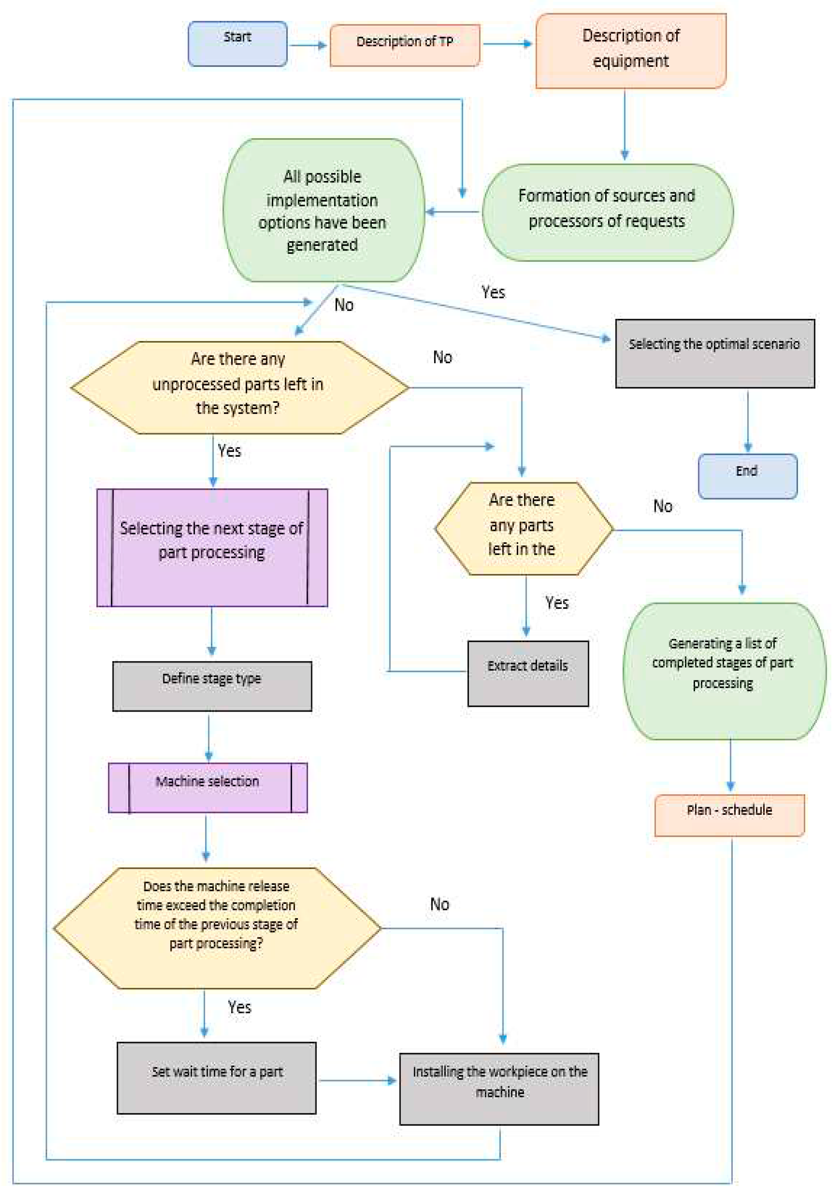
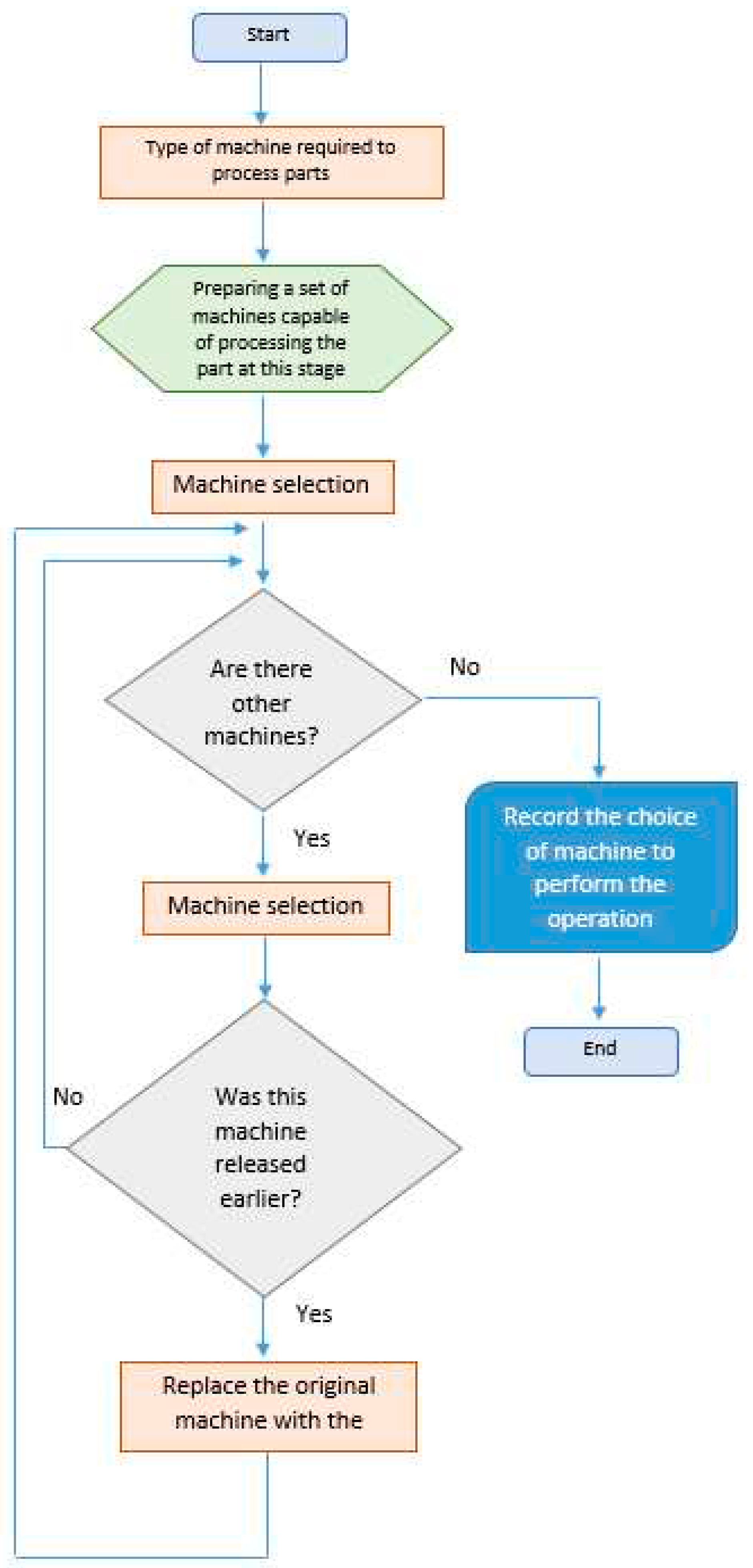
To analyze the maximum possible number of options for technological processing routes for given products, in order to select the optimal work scenario according to the criteria of processing time and cost, the simulation algorithm can be divided into four main stages: processing user input, preparatory stage, the process of generating implementation options and choosing the optimal operating scenario (Figure 2 and Figure 3).
User task: set the following input data for the correct operation of the simulation model:
1. A set of TPs and the number of implementations of each of them, that is, a list consisting of the type of operation, time and cost of implementation.
2. A set of technological equipment - one unit of a given equipment corresponds to one or more types of operations performed.
The preparatory stage consists of creating processors and sources of requests, taking into account the information received from the user.
The main stage is the operation of the ITTP. The process of generating implementation options allows you to generate the largest number of possible implementation scenarios by enumerating the priorities of operations for processing given data. Priorities allow you to set the sequence of selecting applications from sources, that is, parts corresponding to certain technological processes, as well as the sequence of their processing on specified equipment (machines) [49].
The selection of the optimal operating scenario is made using the linear convolution method [50,51].
A simulation model consists of a set of simple elements, designed as basic abstractions. Based on these concepts, it is possible to formulate a basic algorithm for the implemented component of the simulation model.
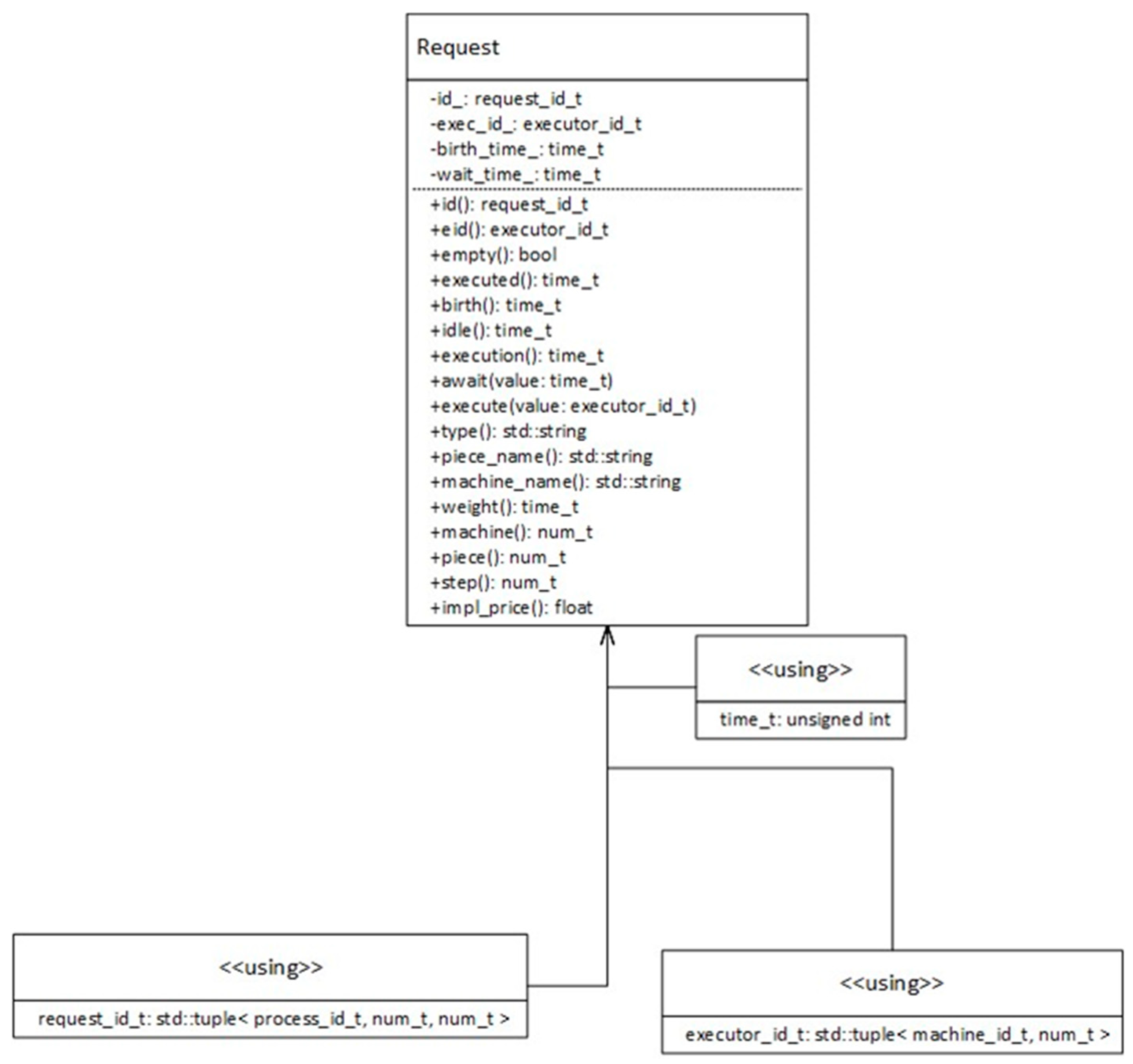
To implement the TP, it is necessary to consistently perform all its stages. Each such stage can be represented in the form of a simulation model application. The application must contain the following information:
1. Number of the TP implemented in the system (represented by the id_ field);
2. Operation number in this TP (id_);
3. TP implementation number (id_);
4. Time of appearance of the application in the system (birth_time_).
New requests in the system await the release of technological equipment capable of performing the corresponding technological operation. When submitting a service request, the waiting time (wait_time_) and the contractor's identifier (exec_id_) are recorded. Thus, for each implementation of a technological process, it is possible to calculate the delay time for performing technological operations. A detailed diagram of the Request class is presented in Figure 4.
TPs are presented in the system in the form of application sources, which records the number of implementations of one of the TPs and generates a unique application identifier. The execution of the TP process is repeated until the specified number of implementations has been completed. Since the TP stages are performed sequentially, each source provides only one application at a time. Thus, the number of requests in the system corresponds to the number of parallel processing processes. This pool of orders can be managed: for example, you can select orders of a certain type of operation.
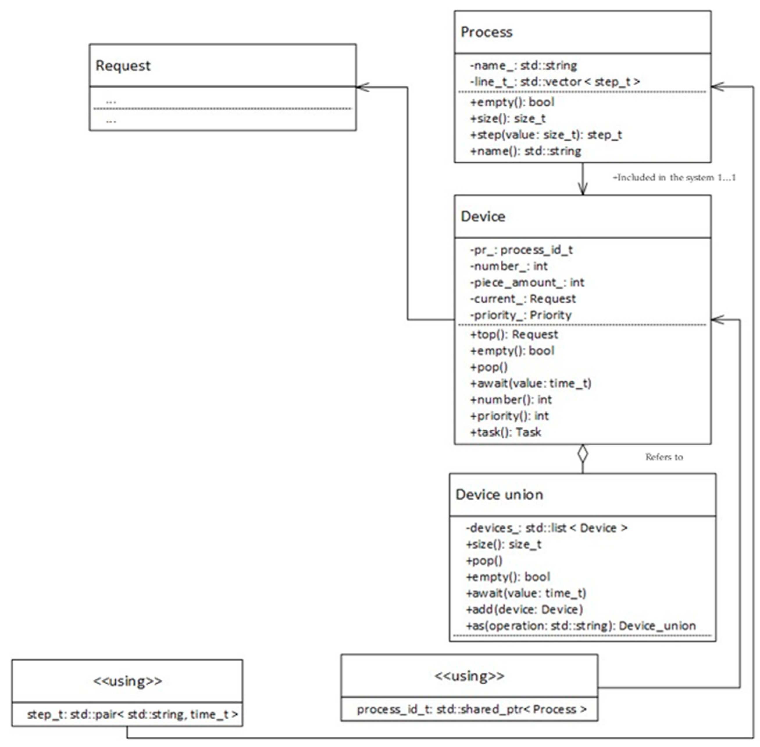
The pool of applications is managed by the Device_union class. Order sources are represented by the Device class, and TPs are represented by the Process class. Figure 5 shows a detailed UML diagram of the listed classes and their relationship with the Request class.
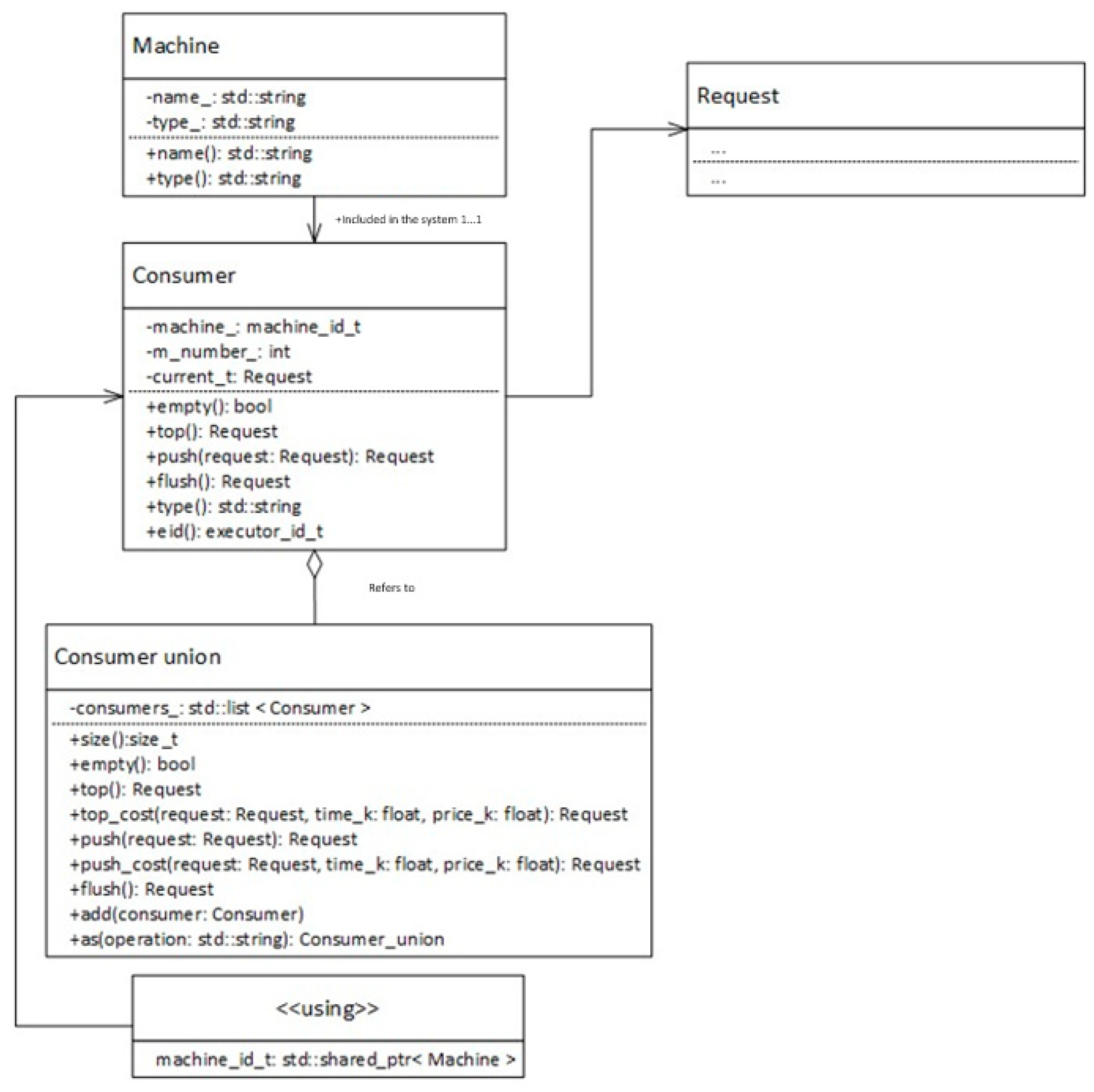
Technological equipment is represented by the Machine class, containing the following information:
1. Name of the process equipment (represented by the name_ field)
2. Types of operations performed (line_)
The resources of a specific piece of technological equipment are managed by the Consumer class, which stores information about the last completed request. The information contained in the application is sufficient to determine the readiness of a certain piece of technological equipment to process the next application.
During the modeling process, the Consumer_union class provides the required unit of technological equipment depending on the selected request, taking into account the priorities and readiness of the units of technological equipment.
Below is a detailed UML diagram of technological equipment and application processors (Figure 6).
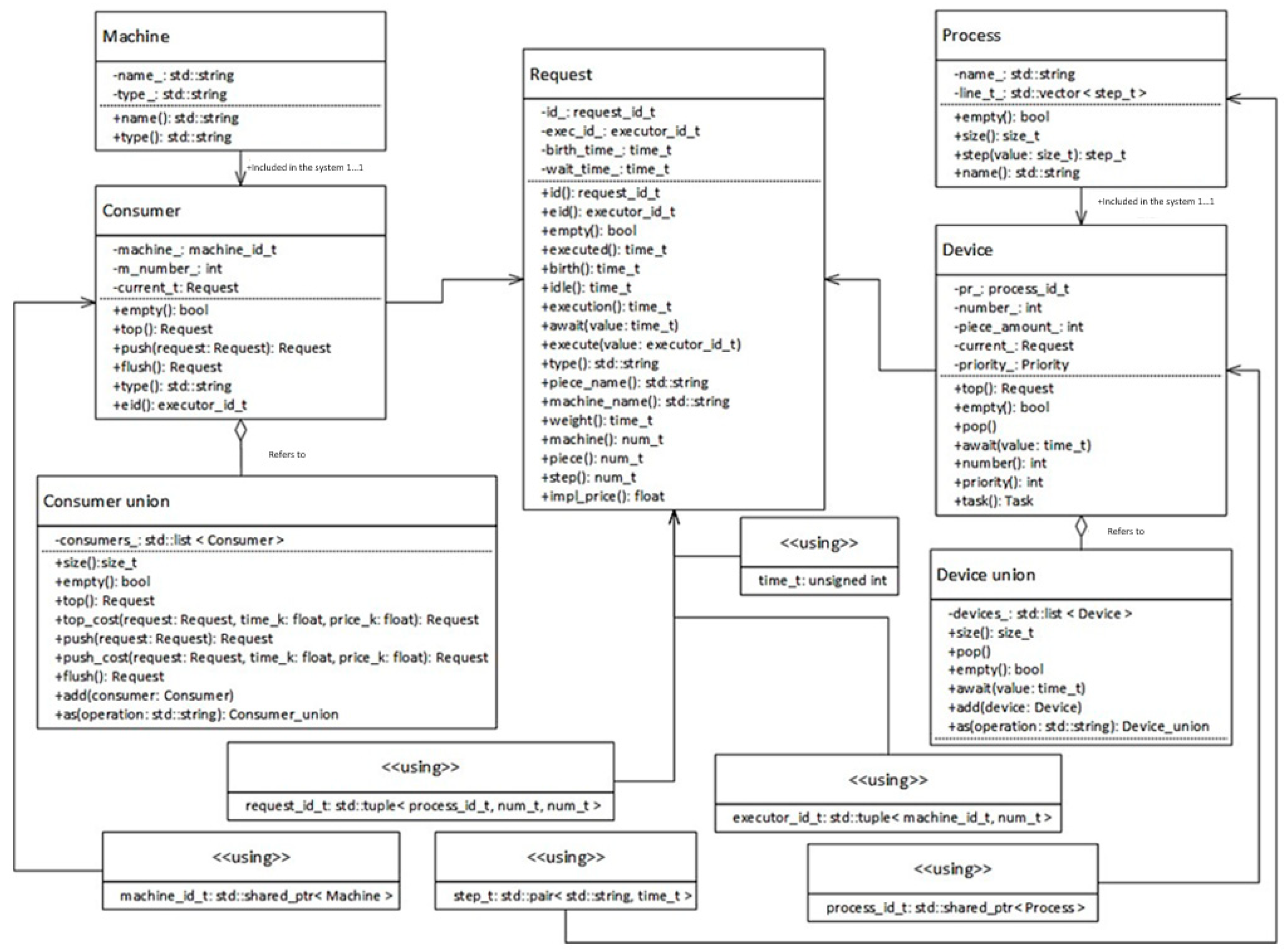
The complete class diagram is shown in Figure 7.
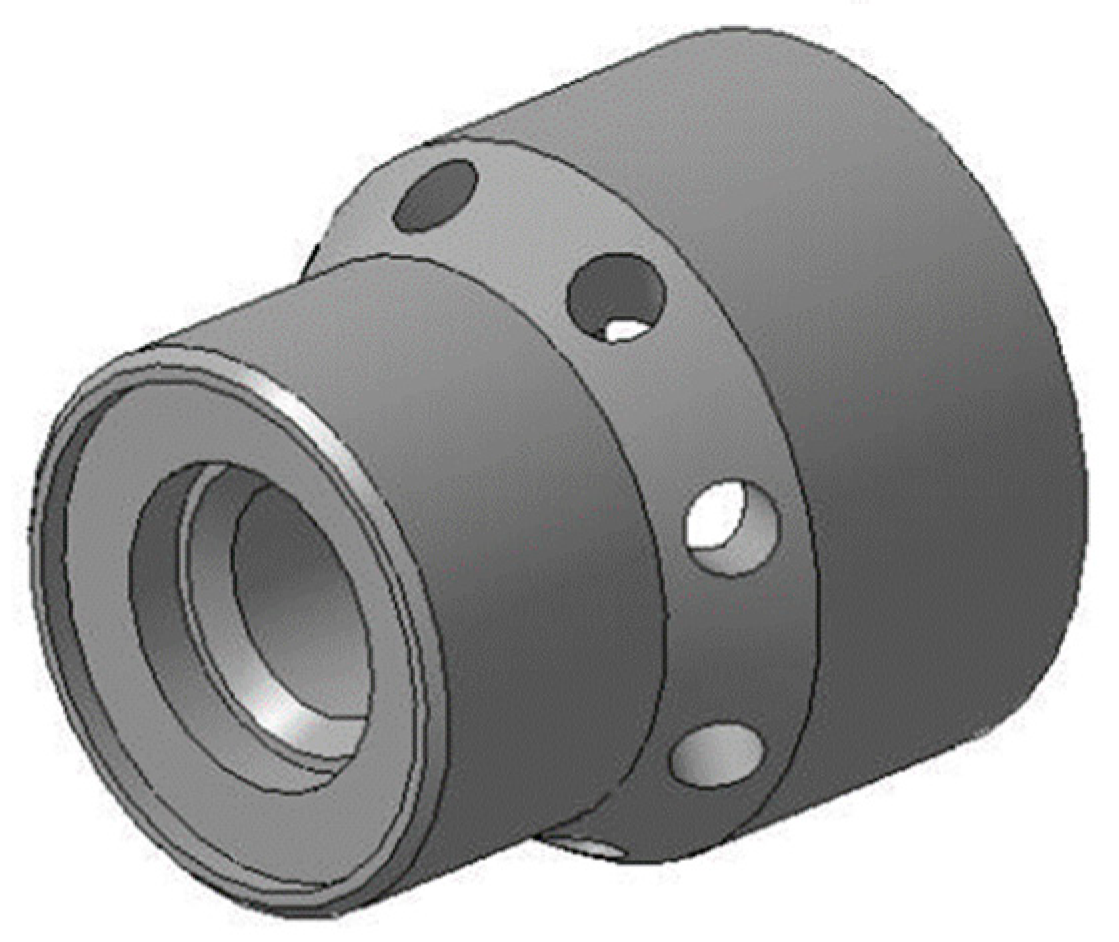
The developed simulation model was used in the process of modeling the technological preparation of production to simulate the manufacture of the “Pusher” part.
The manufactured part “Pusher” (Figure 8) has the following technical parameters:
  • Dimensions: maximum diameter 24mm, length 26mm;
  • Exact dimensions:
    -
    outer diameter 𝜙 24ℎ6 with roughness Ra 0.8;
    -
    internal diameter 𝜙 11𝐻8 with roughness Ra 1.6;
    -
    internal threaded surface M8-7H, roughness Ra 3.2.
  • General tolerances for other dimensions: H14, h14, ±IT14/2.
Four types of machines are involved in the processing route:
  • Thun – universal lathes
  • Tchpu – lathes with numerical control
  • TFNC – turning and milling machines with numerical control
  • KSh – cylindrical grinding machines
Table 1 describes the types of machines and their methods for processing technological elements
In accordance with Table 1, the input data for the simulation model for the given equipment was formulated, presented in Table 2.
Explanation:
- consumer № – identification number of the specified equipment;
- worker – information about the specified equipment;
- machine – name of the specified equipment;
- line – list of types of operations that can be performed on this equipment;
- factor – cost multiplier (the higher the value, the higher the cost of processing parts on this equipment).
For each block of surfaces, the following sequence of processing of the design and technological elements included in their composition was determined:
•MB(1/1): DTE(1Н-1)1 → DTE(2Н/2-1)2 → DTE(2Н/1-1)2 → DTE(2Н/2-1)1
•MB(1/2): DTE(1Н-1)2 → DTE(2Н/1-4)1
•MB(2/1): DTE(2В/1-2)1 → DTE(2В/1-1)2 → DTE(2В/2-1)1 → DTE(1В-1)1
•MB(2/2): DTE(2В/1-2)3 → DTE(2В/1-3)4 → DTE(2В/2-2)2 → DTE(1В-1)2 → DTE(1В-2)3
•MB(4/1): DTE(4В/1-2)1
For the “Pusher” part, the following sequence of processing of surface blocks was defined:
MB(1/2) → MB(2/1) → MB(1/1) → MB(2/2) → MB(4/1)
Technological elements included in the design and technological elements are processed sequentially.
The given surface blocks were divided into final operations (Table 3):
Table 4 shows the relationship between processing methods and their cost and execution time:
In accordance with relation (7) and Table 3, Table 4, the TP input data for the simulation model were formulated, presented in Table 5.
Explanation:
- device № – identification number of the specified TP;
- task – information about a given TP;
- process – name of the specified TP;
- line – list of operations that make up the given TP:
1) time – processing time of a given operation;
2) price – the cost of processing a given operation;
- No. – number of implementations of a given TP
A listing of the final schedule of the simulation model with the main set of cutting tools is presented in Table 6.
Table 6 presents the result of the simulation model in MRD (Machine-Readable Data) format, where:
- id – information about the application being processed;
- name – name of the TP;
- num – part number of the current TP;
- step – number of the operation being performed;
- type – type of operation being performed;
- birth – time of appearance of the current request in the system;
- price – cost of performing the current operation;
- wait – start time of processing the current request;
- executor – information about the equipment on which the application is processed:
1. name – name of the equipment on which the current request is being processed;
2. num – number of the equipment on which the current request is being processed;
3. execution – end time of application processing;
4. impl_price – cost after the application is processed
As a result of simulating the production of the “Pusher” part, the optimal scenario for the operation of the production site was selected according to two criteria of time and cost. The final duration of the production cycle was 471 working hours, the final value of variable costs was 175,000 conventional units, which confirms that the created algorithm and simulation model are adequate under the conditions of a single production. In the future, it is planned to develop a simulation model with an alternative set of cutting tools. Typically, the choice of cutting tool affects the processing time of the part and its cost.

4. Conclusions

In the article, the authors solved the problem of automating the decision-making process of choosing a rational option for implementing a technological process in accordance with the system of preferences of the decision maker. Such problems belong to “discrete” multicriteria selection problems.
To build a new simulation model, the authors used an analysis of various technological processing routes and the technological equipment used. One of the most effective methods for assessing multiple options for technological processes and selecting the most suitable one is simulation modeling of production processes and multi-criteria analysis based on a selected set of criteria.
Unlike the standard structure, the following changes were made to the implemented model:
1. The sources in the model are technological processes (hereinafter referred to as TP). TP represents a strict sequence of operations: from the delivery of blanks and tools from the warehouse to the machines, to the receipt of finished products of a given nomenclature at the warehouse. At the same time, the execution times of all operations are clearly specified.
2. There is no buffer memory.
3. The system cannot skip individual stages of the process, therefore it works flawlessly.
4. The number of devices in the system depends on the specified technological equipment necessary for the implementation of the specified technological processes.
5. During the modeling process, applications are generated - a separate stage of the technological process. At the same time, the system processes one instance of each technological process. Thus, the number of applications in the system does not exceed the total number of technological processes.As a result of the analysis, a simulation model algorithm was developed, UML diagrams were designed describing the structure of the system, classes, their attributes, methods and relationships between objects.
A simulation program has been developed in C++ for single and small-scale production, with the aim of automating the process of technological processing by automatically generating the largest number of work scenarios and further selecting the optimal scenario for the production site according to two criteria of time and cost.
As a result of simulating the production of the “Pusher” part, the final duration of the production cycle was 471 working hours, the final value of variable costs was 175,000 conventional units.

Author Contributions

Conceptualization, T.N. (Tatyana Nikonova) and N.S. (Nadezhda Savelyeva); methodology, O.Zh. (Olga Zharkevich), O.Č. (Olegas Černašėjus) and T.N. (Tatyana Nikonova); software, A.B. (Andrey Berg); validation, G.Zh. (Gulnara Zhetessova), T.N. (Tatyana Nikonova); formal analysis, O.Žh. (Olga Zharkevich) and T.N. (Tatyana Nikonova); investigation, V.Yu. (Vassiliy Yurchenko) and A.B. (Andrey Berg); resources, O.Zh. (Olga Zharkevich) and S.V. (Sergey Vassenkin); data curation, O.Č. (Olegas Černašėjus); writing—original draft preparation, O.Zh. (Olga Zharkevich) and T.N. (Tatyana Nikonova); writing—review and editing, T.N. (Tatyana Nikonova), G.Zh. (Gulnara Zhetessova) and N.S. (Nadezhda Savelyeva); visualization, A.B. (Andrey Berg), E.D. (Essim Dandybaev) and M.B. (Murat Baimuldin); supervision, N.S. (Nadezhda Savelyeva) ; project administration, T.N. (Tatyana Nikonova). All authors have read and agreed to the published version of the manuscript.

Funding

The article was executed within the framework of implementation of IRN grant AP14972804 «Development of software for technological preparation of production on the basis of the formalized design methodology» (Head N.A. Savelyeva).

Institutional Review Board Statement

Not applicable.

Informed Consent Statement

Not applicable.

Data Availability Statement

Not applicable.

Conflicts of Interest

The authors declare no conflict of interest. The funders had no role in the design of the study; in the collection, analyses, or interpretation of data; in the writing of the manuscript; or in the decision to publish the results.

References

  1. Chernorutsky, I.; Kotlyarov, V.; Shyamasundar, R.; Tolstoles, A.; Voinov, N. Implementation of reliable net-centric management of IoT industrial workshop for small-scale production. IOP Conference Series: Materials Science and Engineering, 21–22 November. [CrossRef]
  2. Manzei, C. , Schleupner L., Heinze R. Industrie 4.0 im internationalen Kontext: Kernkonzepte, Ergebnisse, Trends; VDE VERLAG GmbH: Berlin, Germany, 2016; ISBN 3-8007-3671-3. [Google Scholar]
  3. Marcos, M.P.; Pitarch, J.L.; de Prada, C. Integrated Process Re-Design with Operation in the Digital Era: Illustration through an Industrial Case Study. Processes 2021, 9, 1203. [Google Scholar] [CrossRef]
  4. Bako, B.; Božek, P. Trends in simulation and planning of manufacturing companies. International Conference on Manufacturing Engineering and Materials, Novy Smokovec, Slovakia, 6-, Volume 149, pp 571-575. 10 June. [CrossRef]
  5. Chlebus, E.; Krot, K. CAD 3D models decomposition in manufacturing processes. Archives of Civil and Mechanical Engineering 2016, 16, 20–29. [Google Scholar] [CrossRef]
  6. Adam, R.; Kotze, P.; Van der Merwe, A. Acceptance of enterprise resource planning systems by small manufacturing Enterprises. ICEIS 2011 - Proceedings of the 13th International Conference on Enterprise Information Systems, Volume 1, Beijing, China, 8-. 11 June. [CrossRef]
  7. Browne, J.; O'Kelly, M.E.J.; Davies, B.J. Scheduling in a batch or job shop production environment. Engineering Management International 1982, Issue 3, 173–184. [Google Scholar] [CrossRef]
  8. Burdo, G.B. Improving the technological preparations for manufacturing production. Russian Engineering Research volume 2017, 37, 49–56. [Google Scholar] [CrossRef]
  9. Siderska, J. Application of tecnomatix plant simulation for modeling production and logistics processes. Business, Management and Education, 2016. [Google Scholar] [CrossRef]
  10. Dong, S.; Medeiros, D.J. Minimising schedule cost via simulation optimisation: an application in pipe manufacturing. International journal of production research 2012, 50, 831–841. [Google Scholar] [CrossRef]
  11. 11, J. San Cristobal, J.R. Critical Path Definition Using Multicriteria Decision Making: Promethee Method. Journal of Construction Engineering and Management. [CrossRef]
  12. Jato-Espino, D.; Castillo-Lopez, E.; Rodriguez-Hernandez, J.; Canteras-Jordana, J. A review of application of multi-criteria decision making methods in construction. Automation in Construction 2014, 45. 151–162. [CrossRef]
  13. Rosova, A.; Behun, M.; Khouri, S. Case study: the simulation modeling to improve the efficiency and performance of production process. Wireless Networks 2022, 28, 863–872. [Google Scholar] [CrossRef]
  14. Pompeev, K.P.; Timofeeva, O.S.; Yablochnikov, E.I.; Volosatova, E.E. Methods of Parts Digital Models Design for Problems Resolving in Technological Preparation of Production. In: Evgrafov, A.N. (eds) Advances in Mechanical Engineering. Lecture Notes in Mechanical Engineering. Springer, Cham: Saint-Petersburg, Russian Federation, 2022, 129–139. [CrossRef]
  15. Torres-Jimenez, J.; Rangel-Valdez, N.; De-la-Torre, M.; Avila-George, H. An Approach to Aid Decision-Making by Solving Complex Optimization Problems Using SQL Queries. Appl. Sci. 2022, 12, 4569. [Google Scholar] [CrossRef]
  16. Sipser, M. Introduction to the Theory of Computation, 2 edition; Thomson: Boston, USA, 2006; ISBN 0-534-95097-3. [Google Scholar]
  17. Abramov, S.A. Lectures on the complexity of algorithms, ed. 3rd, rev. and additional; MTsNMO: Moscow, Russia, 2020; ISBN 978-5-443-91464-0. [Google Scholar]
  18. Pompeev, K.P.; Timofeeva, O.S.; Yablochnikov, E.I.; Volosatova, E.E. Methods of Parts Digital Models Design for Problems Resolving in Technological Preparation of Production. In: Evgrafov, A.N. (eds) Advances in Mechanical Engineering. Lecture Notes in Mechanical Engineering. Springer, Cham: Saint-Petersburg, Russian Federation, 2022, 129–139. [CrossRef]
  19. Kalyakulin, S.Yu.; Kuzmin, V.V.; Mitin, E.V.; Suldin, S.P.; Tyurbeeva, T.B. Designing the Structure of Technological Processes Based on Synthesis. Mordovia University Bulletin 2018, 28, 77–84. [Google Scholar] [CrossRef]
  20. Khrustaleva, I.N.; Lyubomudrov, S.A.; Chernykh, L.G.; Stepanov, S.N.; Larionova, T.A. Automating production engineering for custom and small-batch production on the basis of simulation modeling. Journal of Physics: Conference Series, 0120. [Google Scholar] [CrossRef]
  21. Ivanov, V.; Botko, F.; Kolos, V.; Pavlenko, I.; Hatala, M.; Antosz, K.; Trojanowska, J. Locating Chart Choice Based on the Decision-Making Approach. Materials 2022, 15, 3557. [Google Scholar] [CrossRef]
  22. Trojanowska, J.; Kolinski, A.; Galusik, D.; Rocha Varela, L. A methodology of improvement of manufacturing productivity through increasing operational efficiency of the production process. Advances in Manufacturing 2018. Springer International Publishing 2018, 1, 23–32. [Google Scholar] [CrossRef]
  23. Araujo, A.F. et al. Development of an intelligent and automated system for lean industrial production, adding maximum productivity and efficiency in the production process. Advances in manufacturing, Springer International Publishing 2018, 1, 131-140. [CrossRef]
  24. Vukelic, D.; Zuperl, U.; Hodolic, J. Complex system for fixture selection, modification, and design. The International Journal of Advanced Manufacturing Technology 2009, 45, 731–748. [Google Scholar] [CrossRef]
  25. Abouel Nasr, E. Al-Ahmari, A.; Khan A.A.; Mian S.H. Integrated system for automation of process, fixture and inspection planning. Journal of the Brazilian Society of Mechanical Sciences and Engineering. [CrossRef]
  26. Liu, M.; Zhou, B.; Li, J.; Li, X.; Bao, J. A Knowledge Graph-Based Approach for Assembly Sequence Recommendations for Wind Turbines. Machines 2023, 11, 930. [Google Scholar] [CrossRef]
  27. Chen, Z. Assembly information model based on knowledge graph. Journal of Shanghai Jiaotong University (Science) 2020, 25, 578–588. [Google Scholar] [CrossRef]
  28. Li, X. Structured modeling of heterogeneous CAM model based on process knowledge graph. The International Journal of Advanced Manufacturing Technology 2018, 96, 4173–4193. [Google Scholar] [CrossRef]
  29. Xu, Z.; Liu, H.; Li, J.; Zhang, Q.; Tang, Y. CKGAT: Collaborative Knowledge-Aware Graph Attention Network for Top-N Recommendation. Appl. Sci. 2022, 12, 1669. [Google Scholar] [CrossRef]
  30. Han, Z.; Mo, R.; Hao, L. Clustering and retrieval of mechanical CAD assembly models based on multi-source attributes information. Robotics and Computer-Integrated Manufacturing. [CrossRef]
  31. Stavropoulos, P.; Papacharalampopoulos, A.; Sabatakakis, K. Data Attributes in Quality Monitoring of Manufacturing Processes: The Welding Case. Appl. Sci. 2023, 13, 10580. [Google Scholar] [CrossRef]
  32. Wang, X.; Liu, M.; Zhong, P.; Zhang, C.; Zhang, D. A Discrete Cooperative Control Method for Production Scheduling Problem of Assembly Manufacturing System. Sustainability 2023, 15, 13785. [Google Scholar] [CrossRef]
  33. Xiong, H.; Shi, Sh.; Ren, D.; Hu, J. A survey of job shop scheduling problem: The types and models. Computers & Operations, 1057. [Google Scholar] [CrossRef]
  34. Mokhtari, H.; Hasani, A. An energy-efficient multi-objective optimization for flexible job-shop scheduling problem, Computers & Chemical Engineering 2017, 104, 339-352. [CrossRef]
  35. Ciurana, J.; Garcia-Romeu, M.L.; Ferrer, I.; Casadesus, M. A model for integrating process planning and production planning and control in machining processes. Robotics and Computer-Integrated Manufacturing. [CrossRef]
  36. García-Leon, A.A.; Dauzère-Pérès, S.; Mati, Ya. An efficient Pareto approach for solving the multi-objective flexible job-shop scheduling problem with regular criteria. Computers & Operations Research. [CrossRef]
  37. Knopp, S.; Dauzère-Pérès, S.; Yugma, C. A batch-oblivious approach for Complex Job-Shop scheduling problems. European Journal of Operational Research 2017, 263(1), 50–61. [Google Scholar] [CrossRef]
  38. Azzouz, A.; Ennigrou, M.; Ben Said, L. A self-adaptive hybrid algorithm for solving flexible job-shop problem with sequence dependent setup time. Procedia Computer Science 2017, 112, 457–466. [Google Scholar] [CrossRef]
  39. Xing, LN.; Chen, YW.; Yang, KW. An efficient search method for multi-objective flexible job shop scheduling problems. Journal of Intelligent Manufacturing 2009, 20, 283–293. [Google Scholar] [CrossRef]
  40. Shen, X.N.; Han, Y.; Fu, J.Z. Robustness measures and robust scheduling for multi-objective stochastic flexible job shop scheduling problems. Soft Computing 2017, 21, 6531–6554. [Google Scholar] [CrossRef]
  41. Fernández Pérez, M.A.; Raupp, F.M.P. A Newton-based heuristic algorithm for multi-objective flexible job-shop scheduling problem. Journal of Intelligent Manufacturing 2016, 27, 409–416. [Google Scholar] [CrossRef]
  42. Moslehi, G.; Mahnam, M. A Pareto approach to multi-objective flexible job-shop scheduling problem using particle swarm optimization and local search. International Journal of Production Economics 2011, 129(1), 14–22. [Google Scholar] [CrossRef]
  43. Kacem, I.; Hammadi, S.; Borne, P. Pareto-optimality approach for flexible job-shop scheduling problems: hybridization of evolutionary algorithms and fuzzy logic. Mathematics and Computers in Simulation. [CrossRef]
  44. Ondov, M.; Rosova, A.; Sofranko, M.; Feher, J.; Cambal, J.; Feckova Skrabulakova, E. Redesigning the Production Process Using Simulation for Sustainable Development of the Enterprise. Sustainability 2022, 14, 1514. [Google Scholar] [CrossRef]
  45. Iassinovski, S.; Artiba, A.; Fagnart, C. A generic production rules-based system for on-line simulation, decision making and discrete process control. International journal of production economics 2008, 112(1), 62–76. [Google Scholar] [CrossRef]
  46. Bernard, A.; Perry, N. Fundamental concepts of product/technology/process informational integration for process modelling and process planning. International Journal of Computer Integrated Manufacturing. [CrossRef]
  47. Shah, D.; Shin, J. Randomized scheduling algorithm for queueing networks. Ann. Appl. Probab. [CrossRef]
  48. Bathaee, M.; Nozari, H.; Szmelter-Jarosz, A. Designing a New Location-Allocation and Routing Model with Simultaneous Pick-Up and Delivery in a Closed-Loop Supply Chain Network under Uncertainty. Logistics 2023, 7, 3. [Google Scholar] [CrossRef]
  49. Malega, P.; Gazda, V.; Rudy, V. Optimization of production system in plant simulation. SIMULATION 2022, 98(4), 295–306. [Google Scholar] [CrossRef]
  50. Kuznetsov, P.M.; Khoroshko, L.L. Digitalization of Multi-Object Technological Projecting in Terms of Small Batch Production. Inventions 2020, 5, 38. [Google Scholar] [CrossRef]
  51. Simunovic, G.; Majdandzic, N.; Simunovic, K.; Lujic, R. Applying of the Typical Technological Operations in the Single Production. AMST’02 Advanced Manufacturing Systems and Technology, 437, 275–281; eds Kulianic, E., Ed.; International Centre for Mechanical Sciences, Springer: Vienna, Austria, 2002. [Google Scholar] [CrossRef]
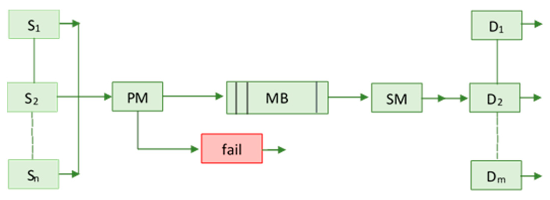
Figure 1. An example of the structure of a queuing system, where И𝑖 (𝑖 = 1 … 𝑛) – sources, PM – production manager, MB – memory buffer, SM – selection manager, П𝑖 (𝑖 = 1 … 𝑚) – device.
Preprints 87173 g001
Figure 2. Simulation model algorithm diagram.
Preprints 87173 g002
Figure 3. Simulation model algorithm diagram.
Preprints 87173 g003
Figure 4. UML diagram of the Request class.
Preprints 87173 g004
Figure 5. UML diagram of technological processes and sources of requests.
Preprints 87173 g005
Figure 6. UML diagram of technological equipment and application processors.
Preprints 87173 g006
Figure 7. UML diagram of the complete simulation model.
Preprints 87173 g007
Figure 8. Solid model of the “Pusher” part.
Preprints 87173 g008
Table 1. Types of machine tools involved and their processing methods.
Machine type Machine type designation Processing method Designation of processing method
1 Тun mach1 tapping threads op1
drilling op2
semi-finish turning op3
rough turning op4
finishing turning op5
2 ТCNC mach2 tapping threads op1
drilling op2
semi-finish turning op3
rough turning op4
finishing turning op5
3 ТFCNC mach3 tapping threads op1
drilling op2
semi-finish turning op3
rough turning op4
finishing turning op5
Pre- op6
grinding
4 KS mach4 Tapping threads op1
Table 2. Analysis of surface blocks for final operations.
Equipment
(:consumer 0:worker (:machine "mach1":line ( "op1" "op2" "op3" "op4" "op5" ):factor 1.0:):)
(:consumer 1:worker (:machine "mach2":line ( "op1" "op2" "op3" "op4" "op5" ) :factor 1.2:):)
(:consumer 2:worker (:machine "mach3":line ( "op1" "op2" "op3" "op4" "op5" ) :factor 1.3:):)
(:consumer 3:worker (:machine "mach4":line ( "op6" ) :factor 1.0:):)
Table 3. Analysis of surface blocks for final operations.
Block of
surfaces
DTE Processing method Designation of processing method
1 MB(1/2) 1 DTE(1Н-1)2 rough turning op4
2 DTE(2Н/1-4)1 re-grinding op6
rough turning op4
semi-finish turning op3
finishing turning op5
2 MB(2/1) 1 DTE(2В/1-2)1 drilling op2
semi-finish turning op3
2 DTE(2В/1-1)2 drilling op2
3 DTE(2В/2-1)1 drilling op2
4 DTE(1В-1)1 rough turning op4
3 MB(1/1) 1 DTE(1Н-1)1 rough turning op4
2 DTE(2Н/2-1)2 rough turning op4
3 DTE(2Н/1-1)2 rough turning op4
4 DTE(2Н/2-1)1 rough turning op4
4 MB(2/2) 1 DTE(2В/1-2)3 drilling op2
semi-finish turning op3
2 DTE(2В/1-3)4 drilling op2
semi-finish turning op3
rough turning op5
3 DTE(2В/2-2)2 drilling op2
semi-finish turning op3
4 DTE(1В-1)2 rough turning op4
5 DTE(1В-2)3 rough turning op4
semi-finish turning op3
5 MB(4/1) 1 DTE(4В/1-2)1 drilling op2
thread cutting op1
Table 4. Correlation of processing methods with cost and execution time.
Designation of processing method Processing method Processing time (working hours) Amount of costs (conventional units)
1 op1 tapping threads 32 4800
2 op2 drilling 18 5600
3 op3 semi-finish turning 12 8200
4 op4 rough turning 20 6800
5 op5 finishing turning 16 7400
6 op6 re-grinding 29 5800
Table 5. Input data of the simulation model for a given technological process.
Technological process
(:device 0:task ( (:process "TP-T":line ( ( "op4" (:time 40:price 13600:) ) ( "op3" (:time 12:price 8200:) ) ( "op5" (:time 16:price 7400:) ) ( "op6" (:time 29:price 5800:) ) ( "op2" (:time 18:price 5600:) ) ( "op3" (:time 12:price 8200:) ) ( "op2" (:time 36:price 11200:) ) ( "op4" (:time 100:price 34000:) ) ( "op2" (:time 18:price 5600:) ) "op3" (:time 12:price 8200:) ) ( "op2" (:time 18:price 5600:) ) ( "op3" (:time 12:price 8200:) ) ( "op5" (:time 16:price 7400:) ) ( "op2" (:time 18:price 5600:) ) ( "op3" (:time 12:price 8200:) ) ( "op4" (:time 40:price 13600:) ) ( "op3" (:time 12:price 8200:) ) ( "op2" (:time 18:price 5600:) ) ( "op1" (:time 32:price 4800:) ) ):) 1 ):)
Table 6. Output data of the simulation model of the technological process of the “Pusher” part.
Simulation Listing
(:id (:name TP-T:num 0:step 0:type op4:):birth 0:price 13600:wait 0:executor (:name mach1:num 0:execution 40:impl_price 13600:):)
(:id (:name TP-T:num 0:step 1:type op3:):birth 40:price 8200:wait 40:executor (:name mach1:num 0:execution 52:impl_price 8200:):)
(:id ():birth 0:price 0:wait 0:executor ():) (:id (:name TP-T:num 0:step 2:type op5:):birth 52:price 7400:wait 52:executor (:name mach1:num 0:execution 68:impl_price 7400:):)
(:id (:name TP-T:num 0:step 4:type op2:):birth 97:price 5600:wait 97:executor (:name mach1:num 0:execution 115:impl_price 5600:):)
(:id (:name TP-T:num 0:step 5:type op3:):birth 115:price 8200:wait 115:executor (:name mach1:num 0:execution 127:impl_price 8200:):)
(:id (:name TP-T:num 0:step 6:type op2:):birth 127:price 11200:wait 127:executor (:name mach1:num 0:execution 163:impl_price 11200:):)
(:id (:name TP-T:num 0:step 7:type op4:):birth 163:price 34000:wait 163:executor (:name mach1:num 0:execution 263:impl_price 34000:):)
(:id (:name TP-T:num 0:step 8:type op2:):birth 263:price 5600:wait 263:executor (:name mach1:num 0:execution 281:impl_price 5600:):)
(:id (:name TP-T:num 0:step 9:type op3:):birth 281:price 8200:wait 281:executor (:name mach1:num 0:execution 293:impl_price 8200:):)
(:id (:name TP-T:num 0:step 10:type op2:):birth 293:price 5600:wait 293:executor (:name mach1:num 0:execution 311:impl_price 5600:):)
(:id (:name TP-T:num 0:step 11:type op3:):birth 311:price 8200:wait 311:executor (:name mach1:num 0:execution 323:impl_price 8200:):)
(:id (:name TP-T:num 0:step 12:type op5:):birth 323:price 7400:wait 323:executor (:name mach1:num 0:execution 339:impl_price 7400:):)
(:id (:name TP-T:num 0:step 13:type op2:):birth 339:price 5600:wait 339:executor (:name mach1:num 0:execution 357:impl_price 5600:):)
(:id (:name TP-T:num 0:step 14:type op3:):birth 357:price 8200:wait 357:executor (:name mach1:num 0:execution 369:impl_price 8200:):)
(:id (:name TP-T:num 0:step 15:type op4:):birth 369:price 13600:wait 369:executor (:name mach1:num 0:execution 409:impl_price 13600:):)
(:id (:name TP-T:num 0:step 16:type op3:):birth 409:price 8200:wait 409:executor (:name mach1:num 0:execution 421:impl_price 8200:):)
(:id (:name TP-T:num 0:step 17:type op2:):birth 421:price 5600:wait 421:executor (:name mach1:num 0:execution 439:impl_price 5600:):)
(:id (:name TP-T:num 0:step 18:type op1:):birth 439:price 4800:wait 439:executor (:name mach1:num 0:execution 471:impl_price 4800:):)
(:id (:name TP-T:num 0:step 3:type op6:):birth 68:price 5800:wait 68:executor (:name mach4:num 3:execution 97:impl_price 5800:):)
(:id (:name TP-T:num 0:step 0:type op4:):birth 0:price 13600:wait 0:executor (:name mach1:num 0:execution 40:impl_price 13600:):)
(:id (:name TP-T:num 0:step 1:type op3:):birth 40:price 8200:wait 40:executor (:name mach1:num 0:execution 52:impl_price 8200:):)
(:id (:name TP-T:num 0:step 2:type op5:):birth 52:price 7400:wait 52:executor (:name mach1:num 0:execution 68:impl_price 7400:):)
(:id (:name TP-T:num 0:step 4:type op2:):birth 97:price 5600:wait 97:executor (:name mach1:num 0:execution 115:impl_price 5600:):)
(:id (:name TP-T:num 0:step 5:type op3:):birth 115:price 8200:wait 115:executor (:name mach1:num 0:execution 127:impl_price 8200:):)
(:id (:name TP-T:num 0:step 6:type op2:):birth 127:price 11200:wait 127:executor (:name mach1:num 0:execution 163:impl_price 11200:):)
(:id (:name TP-T:num 0:step 7:type op4:):birth 163:price 34000:wait 163:executor (:name mach1:num 0:execution 263:impl_price 34000:):)
(:id (:name TP-T:num 0:step 8:type op2:):birth 263:price 5600:wait 263:executor (:name mach1:num 0:execution 281:impl_price 5600:):)
(:id (:name TP-T:num 0:step 9:type op3:):birth 281:price 8200:wait 281:executor (:name mach1:num 0:execution 293:impl_price 8200:):)
(:id (:name TP-T:num 0:step 10:type op2:):birth 293:price 5600:wait 293:executor (:name mach1:num 0:execution 311:impl_price 5600:):)
(:id (:name TP-T:num 0:step 11:type op3:):birth 311:price 8200:wait 311:executor (:name mach1:num 0:execution 323:impl_price 8200:):)
(:id (:name TP-T:num 0:step 12:type op5:):birth 323:price 7400:wait 323:executor (:name mach1:num 0:execution 339:impl_price 7400:):)
(:id (:name TP-T:num 0:step 13:type op2:):birth 339:price 5600:wait 339:executor (:name mach1:num 0:execution 357:impl_price 5600:):)
(:id (:name TP-T:num 0:step 14:type op3:):birth 357:price 8200:wait 357:executor (:name mach1:num 0:execution 369:impl_price 8200:):)
(:id (:name TP-T:num 0:step 15:type op4:):birth 369:price 13600:wait 369:executor (:name mach1:num 0:execution 409:impl_price 13600:):)
(:id (:name TP-T:num 0:step 16:type op3:):birth 409:price 8200:wait 409:executor (:name mach1:num 0:execution 421:impl_price 8200:):)
(:id (:name TP-T:num 0:step 17:type op2:):birth 421:price 5600:wait 421:executor (:name mach1:num 0:execution 439:impl_price 5600:):)
(:id (:name TP-T:num 0:step 18:type op1:):birth 439:price 4800:wait 439:executor (:name mach1:num 0:execution 471:impl_price 4800:):)
(:id (:name TP-T:num 0:step 3:type op6:):birth 68:price 5800:wait 68:executor (:name mach4:num 3:execution 97:impl_price 5800:):)
Res_price:175000 Res_time: 471
Disclaimer/Publisher’s Note: The statements, opinions and data contained in all publications are solely those of the individual author(s) and contributor(s) and not of MDPI and/or the editor(s). MDPI and/or the editor(s) disclaim responsibility for any injury to people or property resulting from any ideas, methods, instructions or products referred to in the content.
Copyright: This open access article is published under a Creative Commons CC BY 4.0 license, which permit the free download, distribution, and reuse, provided that the author and preprint are cited in any reuse.
Prerpints.org logo

Preprints.org is a free preprint server supported by MDPI in Basel, Switzerland.

Subscribe

© 2024 MDPI (Basel, Switzerland) unless otherwise stated