New Solution to 3D Projection in Human-like Binocular Vision

Preprint

Article

New Solution to 3D Projection in Human-like Binocular Vision

Altmetrics

Downloads

169

Views

Comments

A peer-reviewed article of this preprint also exists.

This version is not peer-reviewed

Submitted:

08 October 2023

Posted:

08 October 2023

Read the latest preprint version here

Alerts

Abstract

A human eye has about 120 million rod cells and 6 million cone cells. This huge number of light sensing cells inside a human eye will continuously produce a huge quantity of visual signals which flow into a human brain for daily processing. However, the real-time processing of these visual signals does not cause any fatigue to a human brain. This fact tells us the truth which is to say that human-like vision processes do not rely on complicated formulas to compute depth, displacement, and colors, etc. On the other hand, a human eye is like a PTZ camera. Here, PTZ stands for pan, tilt and zoom. We all know that in computer vision, each set of PTZ parameters (i.e., coefficients of pan, tilt and zoom) requires a dedicated calibration to determine a camera’s projection matrix. Since there is an infinite number of PTZ parameters which could be produced by a human eye, it is unlikely that a human brain stores an infinite number of calibration matrices for each human eye. Therefore, it is an interesting question for us to answer, which is to say whether simpler formulas of computing depth and displacement exist or not. Moreover, these formulas must be calibration friendly (i.e., easy process on the fly or on the go). In this paper, we disclose an important discovery of a new solution to 3D projection in a human-like binocular vision system. The purpose of doing 3D projection in binocular vision is to undertake forward and inverse transformations (or mappings) between coordinates in 2D digital images and coordinates in a 3D analogue scene. The formulas underlying the new solution are accurate, easily computable, easily tunable (i.e., to be calibrated on the fly or on the go) and could be easily implemented by a neural system (i.e., a network of neurons). Experimental results have validated the discovered formulas.

Keywords:

Subject: Computer Science and Mathematics - Computer Vision and Graphics

1. Introduction

We are living inside an ocean of signals. Among all the signals, the most important ones should be the visual signals. Therefore, vision is extremely important to the intelligence of human beings [1]. Similarly, vision is also extremely important to the intelligence of autonomous robots [2]. In the past decades, there have been extensive research activities dedicated to computer vision research. The intensity of such research has been witnessed by the huge amount of conference paper submissions to ICCV (i.e., International Conference on Computer Vision) and CVPR (i.e., International Conference of Computer Vision and Pattern Recognition). However, despite the continuous efforts of research, today’s computer vision is far behind the performance of human vision. Hence, it is important for us to seriously analyze the gaps between computer vision and human vision.

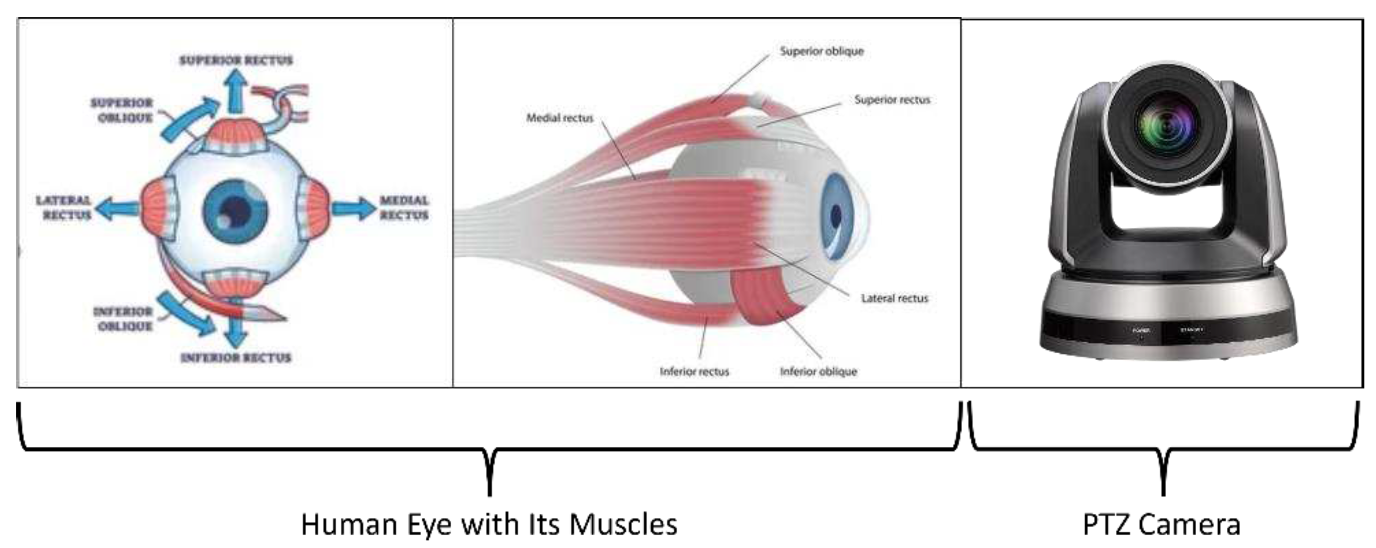
As shown in Figure 1, the motion aspects of a human eye are like a PTZ camera. Here, PTZ stands for pan, tilt and zoom. We know that a human eye can undertake continuous motion and zooming. This implies that a human eye has an infinite number of PTZ parameters (i.e., the coefficients of pan, tilt and zoom). However, our vision processes are not sensitive to the change of PTZ parameters [3,4,5].

On the other hand, a human eye has about 120 million rod cells and 6 million cone cells. These cells are responsible for converting lights into visual signals which will then be processed by a human’s brain. Our daily experience tells us that our brains do not experience any heating-effect and fatigue despite the huge quantity of visual signals under processing in real-time and continuously. This observation leads us to believe that the formulas of the visual processes running inside a human brain must be simple and be suitable for easy and quick implementation by human-brain-like neural systems [6,7].

In view of the above concise analysis, it is reasonable for us to believe that future research direction in computer vision (or robot vision) should be focused on the discovery and invention of the principles and algorithms which are like the formulas behind the visual processes running inside a human brain. Hopefully, the outcomes of this discovery and invention could be implemented in a brain-like digital computer [7].

In this paper, we prove and validate a new solution which will enable autonomous robots, such as car-like robots and humanoid robots, to undertake 3D projection in a human-like binocular vision. The 3D projection includes both forward and inverse projections among positions as well as displacements.

This paper is organized as follows: The technical problem under investigation will be described in Section 2. The background knowledge or related works will be presented in Section 3. The new solution to 3D projection in a human-like binocular vision and its proof will be shown in Section 4. Experimental results for validating the described new solution are included in Section 5. Finally, we conclude this paper in Section 6.

2. Problem Statement

We are living in a three-dimensional space or scene. Similarly, an autonomous robot also manifests its existence or activities in a three-dimensional space or scene. In general, a 3D scene consists of a set of entities which have both global poses (i.e., positions and orientations) and local shapes. If we follow the convention in robotics, each entity in a scene will be assigned a coordinate system (or frame in short) which is called a local coordinate system (or local frame in short). Within a global coordinate system (or global frame in short), an entity’s pose is represented by the position and orientation of its local coordinate system. Within the local coordinate system of an entity, the shape of the entity could be represented by a mesh of triangles or a cloud of points [8].

Therefore, the success of our daily behaviors or activities depends on our mental capabilities of perceiving a three-dimensional space or scene. Similarly, the success of an autonomous robot also depends on its mental capabilities of perceiving a three-dimensional space or scene. More specifically, the intelligence of a human being or an autonomous robot depends on the proper functioning of the outer loop which includes perception, planning and control as shown in Figure 2 [9,10].

It goes without saying that human vision is binocular in nature. Certainly, binocular vision has empowered a human’s mind to achieve impressive intelligent behaviors guided by the perception-planning-control loop. Hence, there is no doubt to us that it is an important research topic which aims at achieving human-like intelligent behaviors by autonomous robots under the guidance of human-like binocular vision [11].

With visual signals as input, two important tasks of binocular vision are to provide information and knowledge about the answers to these two general questions which are: a) what have been seen? and b) where are the entities seen? Figure 3 illustrates these two related questions faced by a binocular vision system. Please take note that a third popular question in binocular vision is: what are the shapes of the entities seen? However, the solution to the first question is also the solution to this third question. Hence, without loss of generality, it is not necessary to specifically highlight this third popular question.

As shown in Figure 3, the first question refers to the problem of entity detection (e.g., object detection), entity identification (e.g., object identification), or entity classification (e.g., object classification). The second question refers to the problem of 2D/3D localization or 2D/3D reconstruction. In this paper, the problem under investigation is to develop a better solution which provides the answer to the second question.

3. Related Works

The problem under investigation in this paper belongs to computer vision. which is a well-established discipline in science and engineering [12,13,14,15,16,17,18]. Since computer vision is a very important module or perception system inside autonomous robots, the problem under investigation is also related to robotics, in which an interesting concept is about forward and inverse kinematics. In this section, we summarize the background knowledge (or related works) in robotics and computer vision, which serve as the foundation of the new solution presented in this paper.

3.1. Concept of Kinematic Chain

In robotics [19,20,21,22], the study of kinematics starts with the assignment of a local coordinate system (or frame) to each rigid body (e.g., a link in a robot). In this way, a series of links in a robot arm manipulator become a kinematic chain. Hence, the topic of kinematics in robotics is about the study the motion relationships among the local coordinate systems assigned to the links of a robot arm manipulator.

In general, a vision system must involve the use of at least one camera which includes a lens (i.e. a rigid body), an imaging sensor array (i.e. a rigid body) and a digital image matrix (i.e. a virtual rigid body). Also, a camera must be mounted on a robot, a machine, or a supporting ground, each of which could be considered as a rigid body. Hence, a camera should be considered as a kinematic chain. In this way, we could talk about the kinematics of a camera, a monocular vision, or a binocular vision.

For example, in Figure 3, a binocular vision system could be considered as the sum of two monocular vision systems. Each monocular vision system consists of a single camera. If we look at the left camera, we could see its kinematic chain which includes the motion transformations such as: transformation from world frame to left-camera frame, transformation from left-camera frame to analogue-image frame, and transformation from analogue-image frame to digital-image frame.

3.2. Forward Projection Matrix of Camera

A single camera is the basis of a monocular vision. Before we could understand the 2D forward and inverse projections of monocular vision, it is necessary for us to know the details of a camera’s forward projection matrix.

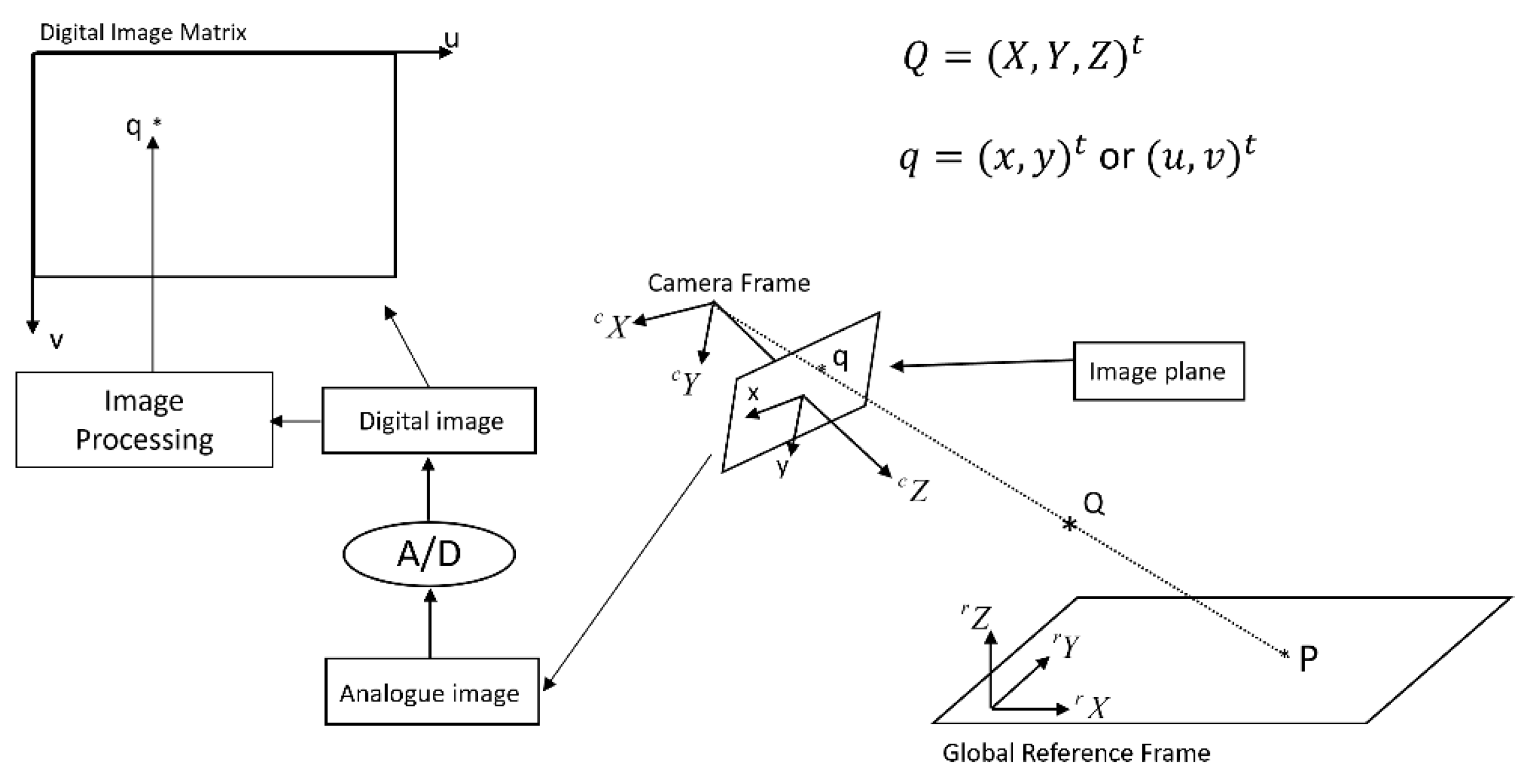
Refer to Figure 4. With the use of the terminology of kinematic chain, the derivation of camera matrix starts with the transformation from reference frame to camera frame. If the coordinates of point Q with respect to reference frame are

(X, Y, Z)

, the coordinates

(X_{c}, Y_{c}, Z_{c})

of the same point Q with respect to camera frame will be [12]:

[\begin{matrix} X_{c} \\ Y_{c} \\ \begin{matrix} Z_{c} \\ 1 \end{matrix} \end{matrix}] = [\begin{matrix} r_{11} & r_{12} & \begin{matrix} r_{13} & t_{x} \end{matrix} \\ r_{21} & r_{22} & \begin{matrix} r_{23} & t_{y} \end{matrix} \\ \begin{matrix} r_{31} \\ 0 \end{matrix} & \begin{matrix} r_{32} \\ 0 \end{matrix} & \begin{matrix} \begin{matrix} r_{33} \\ 0 \end{matrix} & \begin{matrix} t_{z} \\ 1 \end{matrix} \end{matrix} \end{matrix}] \cdot [\begin{matrix} X \\ Y \\ \begin{matrix} Z \\ 1 \end{matrix} \end{matrix}]

(1)

where rotation matrix

{r_{i j}, i \in [1,3], j \in [1,3]}

represents the orientation of reference frame with respect to camera frame, and translation vector

{(t_{x}, t_{y}, t_{z})}^{t}

represents the position of reference frame’s origin with respect to camera frame.

Inside the camera frame, the transformation from the coordinates

(X_{c}, Y_{c}, Z_{c})

of point Q to the analogue image coordinates

{(x, y)}^{t}

of point q will be:

[\begin{matrix} s \cdot x \\ s \cdot y \\ s \end{matrix}] = [\begin{matrix} f & 0 & \begin{matrix} 0 & 0 \end{matrix} \\ 0 & f & \begin{matrix} 0 & 0 \end{matrix} \\ 0 & 0 & \begin{matrix} 1 & 0 \end{matrix} \end{matrix}] \cdot [\begin{matrix} X_{c} \\ Y_{c} \\ \begin{matrix} Z_{c} \\ 1 \end{matrix} \end{matrix}]

(2)

where

f

is the focal length of the camera and

s

is a scaling factor.

By default, we are using digital cameras. Hence, an analogue image is converted into its corresponding digital image. Such process of digitization results in the further transformation from analogue image frame to digital image frame. This transformation is described by the following equation:

[\begin{matrix} s \cdot u \\ s \cdot v \\ s \end{matrix}] = [\begin{matrix} \frac{1}{∆ u} & 0 & u_{0} \\ 0 & \frac{1}{∆ v} & v_{0} \\ 0 & 0 & 1 \end{matrix}] \cdot [\begin{matrix} s \cdot x \\ s \cdot y \\ s \end{matrix}]

(3)

where

{(u, v)}^{t}

are the digital image coordinates of point q,

∆ u

is the width of a pixel (i.e., a digital image’s pixel density in horizontal direction),

∆ v

is the height of a pixel (i.e., a digital image’s pixel density in vertical direction), and

{(u_{0}, v_{0})}^{t}

are the digital image coordinates of the intersection point between the optical axis (i.e., camera frame’s Z axis) and the image plane (note: this point is also called a camera’s principal point).

Now, by substituting Equation 1 and Equation 2 into Equation 3, we will be able to obtain the following equation [16]:

[\begin{matrix} s \cdot u \\ s \cdot v \\ s \end{matrix}] = C_{f} \cdot [\begin{matrix} X \\ Y \\ \begin{matrix} Z \\ 1 \end{matrix} \end{matrix}]

(4)

with

C_{f} = [\begin{matrix} \frac{f}{∆ u} & 0 & \begin{matrix} u_{0} & 0 \end{matrix} \\ 0 & \frac{f}{∆ v} & \begin{matrix} v_{0} & 0 \end{matrix} \\ 0 & 0 & \begin{matrix} 1 & 0 \end{matrix} \end{matrix}] \cdot [\begin{matrix} r_{11} & r_{12} & \begin{matrix} r_{13} & t_{x} \end{matrix} \\ r_{21} & r_{22} & \begin{matrix} r_{23} & t_{y} \end{matrix} \\ \begin{matrix} r_{31} \\ 0 \end{matrix} & \begin{matrix} r_{32} \\ 0 \end{matrix} & \begin{matrix} \begin{matrix} r_{33} \\ 0 \end{matrix} & \begin{matrix} t_{z} \\ 1 \end{matrix} \end{matrix} \end{matrix}]

(5)

where matrix

C_{f}

is called a camera’s forward projection matrix which is a

3 \times 4

matrix.

3.3. 3D Forward Projection of Monocular Vision

A monocular vision system uses a single camera. Its kinematic chain is the same as the one shown in Figure 4. Most importantly, Equation 4 describes 3D forward projection of a monocular vision system, in which 3D coordinates

{(X, Y, Z)}^{t}

are projected into 2D digital image coordinates

{(u, v)}^{t}

3.4. 3D Inverse Projection of Monocular Vision

From the viewpoint of pure mathematics, Equation 4 could re-written into the following form:

[\begin{matrix} k \cdot X \\ k \cdot Y \\ \begin{matrix} k \cdot Z \\ k \end{matrix} \end{matrix}] = C_{i} \cdot [\begin{matrix} u \\ v \\ 1 \end{matrix}]

(6)

with

{C_{i} = (C_{f}^{t} \cdot C_{f})}^{- 1} \cdot C_{f}^{t}

(7)

and

k = 1 / s

In theory, Equation 6 describes 3D inverse projection of a monocular vision system. In practice, Equation 6 could be graphically represented by an artificial neural network which serves as predictor. The input layer consists of

{(u, v, 1)}^{t}

and the output layer consists of

{(X, Y, Z)}^{t}

. Matrix

C_{i}

contains the weighting coefficients. Hence, it is clear to us that different matrix

C_{i}

will enable the prediction of coordinates

{(X, Y, Z)}^{t}

on a different planar surface. Most importantly, matrix

C_{i}

could be obtained by a top-down process of calibration or a bottom-up process of tuning (i.e., optimization). Therefore, Equation 6 serves as a good example which helps us to understand the difference between machine learning and machine calibration (or tuning).

Although

C_{i}

is a

4 \times 3

matrix, it is not possible to use Equation 6 to generally compute 3D coordinates

{(X, Y, Z)}^{t}

in an analogue scene from 2D index coordinates

{(u, v)}^{t}

(i.e., u is column index while v is row index) in a digital image. However, the philosophy behind Equation 6 has inspired us to discover a similar, but very useful, 3D inverse projection of binocular vision which will be described in Section 4.

3.5. 2D Forward Projection of Monocular Vision

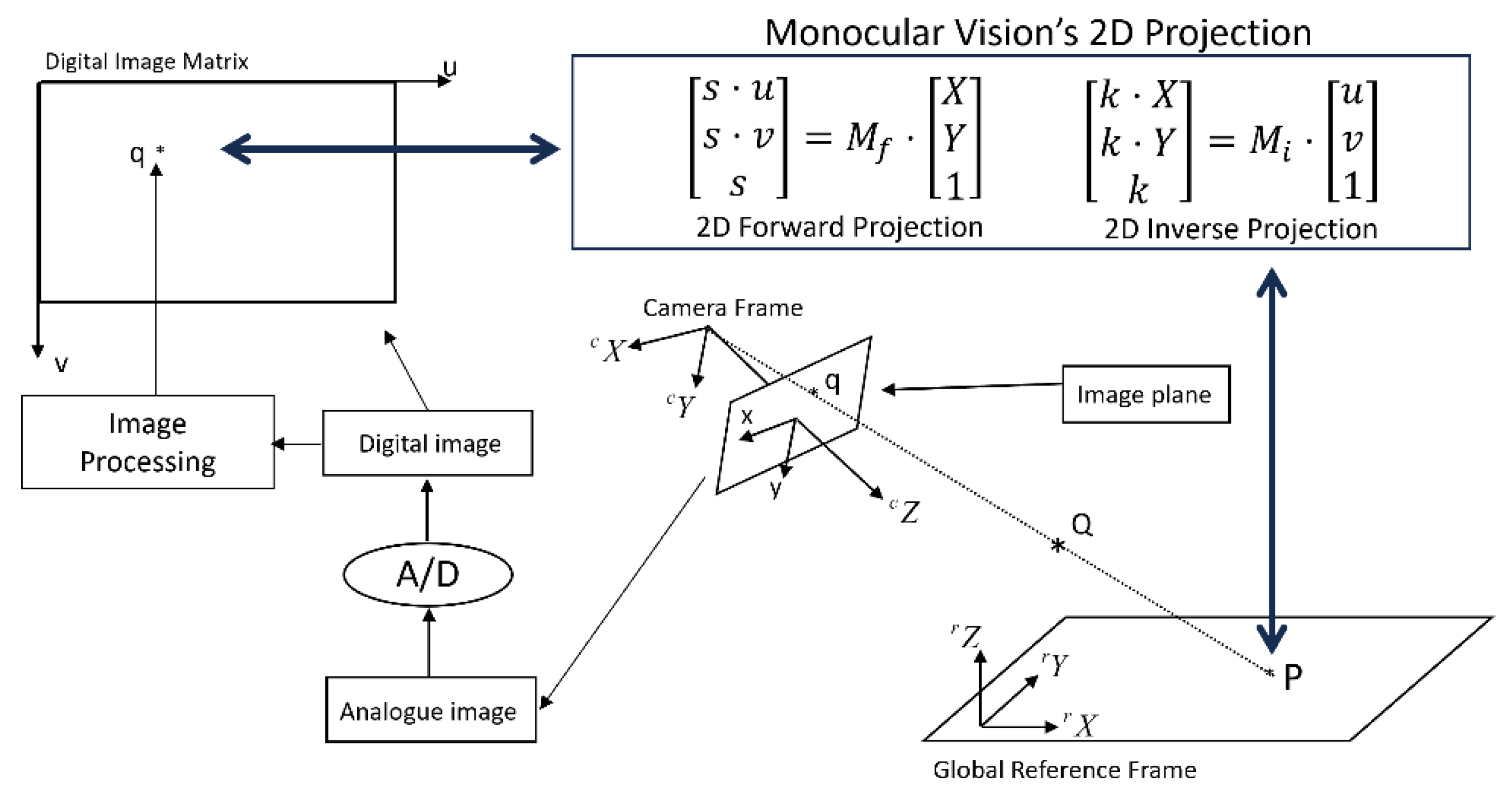
Refer to Figure 4. If we consider the points or locations on the OXY plane of reference frame, Z coordinate in Equation 4 becomes zero. Hence, Equation 4 could be re-written into the following form:

[\begin{matrix} s \cdot u \\ s \cdot v \\ s \end{matrix}] = M_{f} \cdot [\begin{matrix} X \\ Y \\ 1 \end{matrix}]

(8)

where matrix

M_{f}

is the version of matrix

C_{f}

after removing its third column because Z is equal to zero. Clearly, matrix

M_{f}

is a

2 \times 2

matrix and is invertible. As shown in Figure 8, Equation 8 actually describes the 2D forward projection from coordinates

{(X, Y)}^{t}

on a plane of reference frame into digital image coordinates

{(u, v)}^{t}

of monocular vision.

3.6. 2D Inverse Projection of Monocular Vision

Now, by inverting Equation 8, we could easily obtain the following result:

[\begin{matrix} k \cdot X \\ k \cdot Y \\ k \end{matrix}] = M_{i} \cdot [\begin{matrix} u \\ v \\ 1 \end{matrix}]

(9)

with

M_{i} = {(M_{f}^{t} \cdot M_{f})}^{- 1} \cdot M_{f}^{t}

(10)

where matrix

M_{i}

is also a

2 \times 2

matrix.

It goes without saying that Equation 8 and Equation 9 fully describe 2D forward and inverse projections of a monocular vision system as shown in Figure 5.

3.7. Textbook Solution of Computing 3D Coordinates from Binocular Vision

As we have mentioned above, in theory, it is not possible to generally compute 3D coordinates in an analogue scene from 2D index coordinates in a digital image. This fact is proven by Equation 4 and Equation 6 because there is a shortage of one constraint.

It is well-known in computer vision textbooks [12,13,14,15,16,17,18] that one additional constraint is needed if we want to fully determine 3D coordinates in a scene in general. The popular solution to add one extra constraint is to introduce a second camera. This solution results in what is called a binocular vision system as shown in Figure 3.

Now, by applying Equation 4 to Figure 3, we will have the following two relationships:

[\begin{matrix} s_{l} \cdot u_{l} \\ s_{l} \cdot v_{l} \\ s_{l} \end{matrix}] = C_{f}^{l} \cdot [\begin{matrix} X \\ Y \\ \begin{matrix} Z \\ 1 \end{matrix} \end{matrix}]

(11)

and

[\begin{matrix} s_{r} \cdot u_{r} \\ s_{r} \cdot v_{r} \\ s_{r} \end{matrix}] = C_{f}^{r} \cdot [\begin{matrix} X \\ Y \\ \begin{matrix} Z \\ 1 \end{matrix} \end{matrix}]

(12)

where

C_{f}^{l} = {c_{i j}^{l}, i \in [1,3], j \in [1,4]}

and

C_{f}^{r} = {c_{i j}^{r}, i \in [1,3], j \in [1,4]}

are respectively the forward projection matrices of left and right cameras,

{(u_{l}, v_{l})}^{t}

are index coordinates of point b which is the image of point Q inside left camera, and

{(u_{r}, v_{r})}^{t}

are index coordinates of point a which is the image of point Q inside right camera.

If define matrix U and vector V as follows:

U = [\begin{matrix} (c_{11}^{l} - c_{31}^{l} \cdot u_{l}) & (c_{12}^{l} - c_{32}^{l} \cdot u_{l}) & (c_{13}^{l} - c_{33}^{l} \cdot u_{l}) \\ (c_{21}^{l} - c_{31}^{l} \cdot v_{l}) & (c_{22}^{l} - c_{32}^{l} \cdot v_{l}) & (c_{23}^{l} - c_{33}^{l} \cdot v_{l}) \\ \begin{matrix} (c_{11}^{r} - c_{31}^{r} \cdot u_{r}) \\ (c_{21}^{r} - c_{31}^{r} \cdot v_{r}) \end{matrix} & \begin{matrix} (c_{12}^{r} - c_{32}^{r} \cdot u_{r}) \\ (c_{22}^{r} - c_{32}^{r} \cdot v_{r}) \end{matrix} & \begin{matrix} (c_{13}^{r} - c_{33}^{r} \cdot u_{r}) \\ (c_{23}^{r} - c_{33}^{r} \cdot v_{r}) \end{matrix} \end{matrix}]

(13)

and

V = [\begin{matrix} u_{l} - c_{14}^{l} \\ v_{l} - c_{24}^{l} \\ \begin{matrix} u_{r} - c_{14}^{r} \\ v_{r} - c_{24}^{r} \end{matrix} \end{matrix}]

(14)

the elimination of

s_{l}

and

s_{r}

in Equation 11 and Equation 12, followed by the summation of resulting equations, will yield the following result:

U \cdot [\begin{matrix} X \\ Y \\ Z \end{matrix}] = V

(15)

Finally, the pseudo-inverse of matrix U will result in the following formula for the computation of 3D coordinates

{(X, Y, Z)}^{t}

[\begin{matrix} X \\ Y \\ Z \end{matrix}] = {(U^{t} \cdot U)}^{- 1} (U^{t} \cdot V)

(16)

Equation 16 is the textbook solution for computing 3D coordinates if a matched pair of

{(u_{l}, v_{l}), (u_{r}, v_{r})}

are given.

Clearly, Equation 16 tells us that this way of computing each set of 3D coordinates requires a lot of computational resources. If there is a huge quantity of pixels inside the images of a binocular vision system, such computation will consume a lot of energy.

However, our eyes do not cause fatigue to our brains. Certainly, there must be a simpler way of precisely computing 3D coordinates inside a human-like binocular vision system. We will present in the next section an interesting solution, which does not require expensive computational resources, and consequently will consume much less energy.

4. Equations of 3D Projection in Human-like Binocular Vision

Equation 8 and Equation 9 described in Section 3 indicates that a monocular vision system has both forward and inverse projections between 2D digital images and 2D planar surfaces. Especially, both equations do not require expensive computational resources. Naturally, we are curious to know whether such beautiful result do exist for a binocular vision or not.

In the remaining part of this section, we are going to prove the existence of similar solution for both forward and inverse projections in a binocular vision system. First, we will start to prove the equation of 3D inverse projection of binocular vision. Then, the result of 3D inverse projection will help us to prove the equation of 3D forward projection of binocular vision.

4.1. Equation of 3D Inverse Projection of Position in Binocular Vision

The application of Equation 6 to Figure 3 will yield the following two relationships:

[\begin{matrix} k_{l} \cdot X \\ k_{l} \cdot Y \\ \begin{matrix} k_{l} \cdot Z \\ k_{l} \end{matrix} \end{matrix}] = C_{i}^{l} \cdot [\begin{matrix} u_{l} \\ v_{l} \\ 1 \end{matrix}]

(17)

and

[\begin{matrix} k_{r} \cdot X \\ k_{r} \cdot Y \\ \begin{matrix} k_{r} \cdot Z \\ k_{r} \end{matrix} \end{matrix}] = C_{i}^{r} \cdot [\begin{matrix} u_{r} \\ v_{r} \\ 1 \end{matrix}]

(18)

where

C_{i}^{l} = {a_{i j}^{l}, i \in [1,3], j \in [1,4]}

and

C_{i}^{r} = {a_{i j}^{r}, i \in [1,3], j \in [1,4]}

are respectively the inverse projection matrices of left and right cameras,

{(u_{l}, v_{l})}^{t}

are index coordinates of point b which is the image of point Q inside left camera, and

{(u_{r}, v_{r})}^{t}

are index coordinates of point a which is the image of point Q inside right camera.

Now, if we define matrix

B_{i}

as follows:

B_{i} = [\begin{matrix} a_{11}^{l} & a_{12}^{l} & \begin{matrix} a_{11}^{r} & a_{12}^{r} & a_{13}^{l} + a_{13}^{r} \end{matrix} \\ a_{21}^{l} & a_{22}^{l} & \begin{matrix} a_{21}^{r} & a_{22}^{r} & a_{23}^{l} + a_{23}^{r} \end{matrix} \\ \begin{matrix} a_{31}^{l} \\ a_{41}^{l} \end{matrix} & \begin{matrix} a_{32}^{l} \\ a_{42}^{l} \end{matrix} & \begin{matrix} \begin{matrix} a_{31}^{r} & a_{32}^{r} & a_{33}^{l} + a_{33}^{r} \end{matrix} \\ \begin{matrix} a_{41}^{r} & a_{42}^{r} & a_{43}^{l} + a_{43}^{r} \end{matrix} \end{matrix} \end{matrix}]

(19)

the combination (i.e., sum) of Equation 17 and Equation 18 will yield the following result:

[\begin{matrix} k \cdot X \\ k \cdot Y \\ \begin{matrix} k \cdot Z \\ k \end{matrix} \end{matrix}] = B_{i} \cdot [\begin{matrix} u_{l} \\ v_{l} \\ \begin{matrix} u_{r} \\ v_{r} \\ 1 \end{matrix} \end{matrix}]

(20)

where

k = k_{l} + k_{r}

Interestingly, Equation 20 is the equation of 3D inverse projection of a binocular vision system. Matrix

B_{i}

is the 3D inverse projection matrix of binocular vision. This matrix is a

4 \times 5

matrix with 20 elements inside. Due to the presence of scaling factor

k

, there is only 19 independent elements inside matrix

B_{i}

which could be determined by a calibration process.

For example, a set of known values

{(X, Y, Z), (u_{l}, v_{l}), (u_{r}, v_{r})}

will yield three constraints from Equation 20. Hence, with a list of 17 sets of

{(X, Y, Z), (u_{l}, v_{l}), (u_{r}, v_{r})}

, matrix

B_{i}

could be fully computed in advance, on the fly, or on the go.

Interestingly, in the context of a binocular vision system mounted inside the head of a humanoid robot which has dual arms as well as dual multiple-fingered hands, the visually observed fingertips of a humanoid robot’s hands could easily supply a list of known values

{(X, Y, Z), (u_{l}, v_{l}), (u_{r}, v_{r})}

. These values will allow a humanoid robot to achieve the scenario of doing periodical calibration on the fly or on the go.

4.2. Equation of 3D Forward Projection of Position in Binocular Vision

Now, if we compute the pseudo-inverse of matrix

B_{i}

, Equation 20 will become:

[\begin{matrix} {s \cdot u}_{l} \\ s \cdot v_{l} \\ \begin{matrix} {s \cdot u}_{r} \\ s \cdot v_{r} \\ s \end{matrix} \end{matrix}] = B_{f} \cdot [\begin{matrix} X \\ Y \\ \begin{matrix} Z \\ 1 \end{matrix} \end{matrix}]

(21)

where

s = 1 / k

and

B_{f} = {(B_{i}^{t} \cdot B_{i})}^{- 1} \cdot B_{i}^{t}

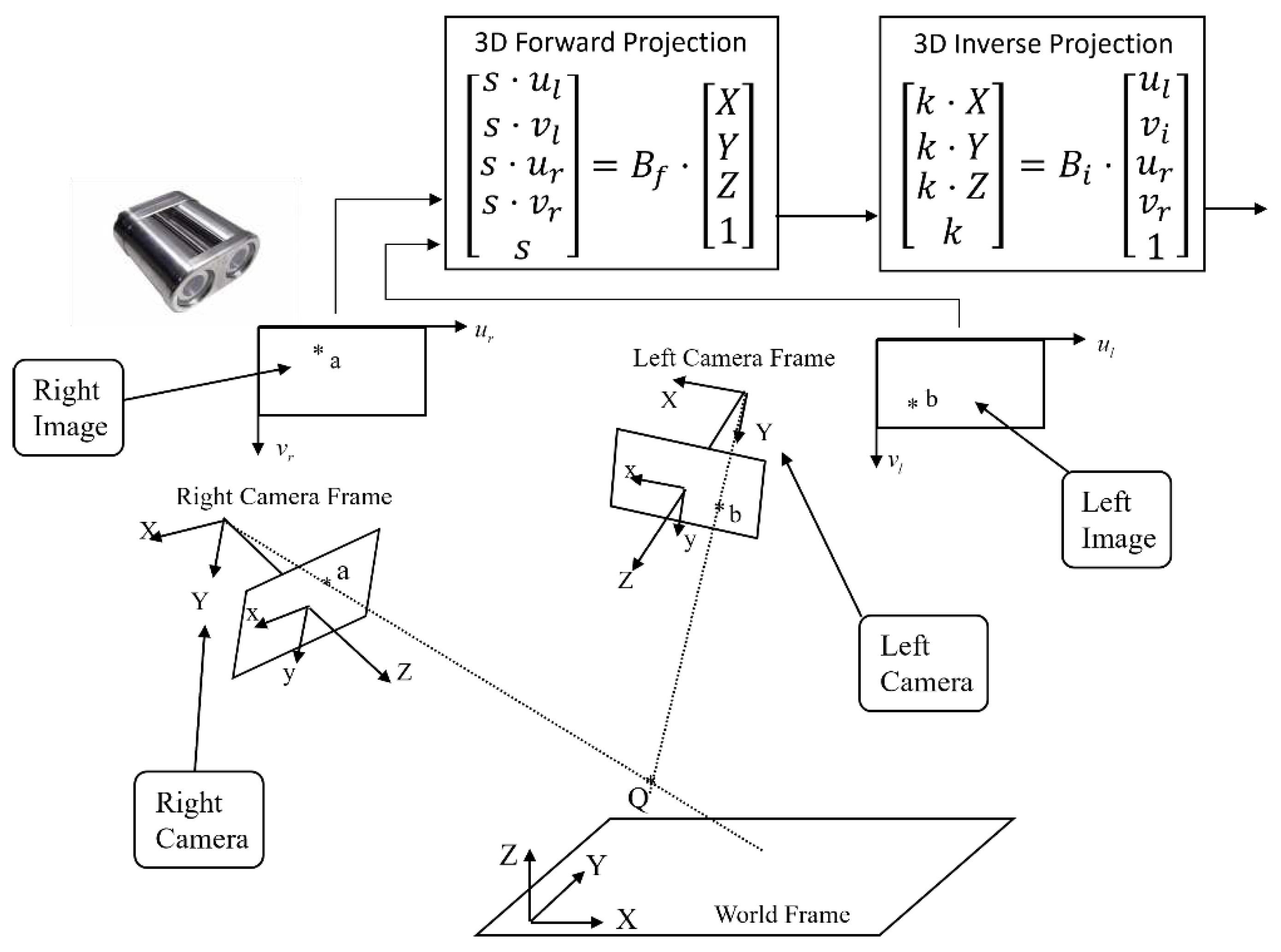
Equation 21 is the equation of 3D forward projection of binocular vision, in which matrix

B_{f}

is 3D forward projection matrix of binocular vision as shown in Figure 6.

4.3. Equation of 3D Inverse Projection of Displacement of Binocular Vision

Mathematically, Equation 20 is differentiable. Moreover, the relationship between derivatives

{(\frac{d X}{d t}, \frac{d Y}{d t}, \frac{d Z}{d t})}^{t}

and derivatives

{(\frac{d u_{l}}{d t}, \frac{d v_{l}}{d t}, \frac{d u_{r}}{d t}, \frac{d v_{r}}{d t})}^{t}

will be the same as the relationship between variations

{(∆ X, ∆ Y, ∆ Z)}^{t}

and variations

{(∆ u_{l}, ∆ v_{l}, ∆ u_{r}, ∆ v_{r})}^{t}

. This is because matrix

B_{f}

is a constant matrix if the kinematic chain of binocular vision remains unchanged [20].

Now, we remove the last column of matrix

B_{i}

(NOTE:

B_{i} = {b_{i j}, i \in [1,4], j \in [1,5]}

) and use the remaining elements to define a new matrix

D_{i}

as follows:

D_{i} = {d_{i j} = {\frac{1}{k} \cdot b}_{i j}, i \in [1,4], j \in [1,4]}

. In this way, the differentiation of Equation 20 will yield the following result [20]:

[\begin{matrix} ∆ X \\ ∆ Y \\ ∆ Z \end{matrix}] = D_{i} \cdot [\begin{matrix} ∆ u_{l} \\ ∆ v_{l} \\ \begin{matrix} ∆ u_{r} \\ ∆ v_{r} \end{matrix} \end{matrix}]

(22)

Equation 22 represents 3D inverse projection of displacement in a binocular vision system. Since scale

k

is not constant, matrix

D_{i}

will not be a constant matrix. However, in practice, we could treat any instance of matrix

D_{i}

as a constant matrix. In this way, Equation 22 could be used inside an autonomous robot’s outer loop of perception, planning and control as shown in Figure 2.

Therefore, Equation 22 is an iterative solution to 3D inverse projection of displacement in binocular vision. The application of Equation 22 to robot guidance is an advantage. This is because Equation 22 will make perception-planning-control loop not to be sensitive to both noise and changes of internal parameters of a binocular vision system.

4.4. Equation of 3D Forward Projection of Displacement of Binocular Vision

Now, by doing a simple pseudo-inverse of matrix

D_{i}

, Equation 22 will allow us to obtain the following equation of 3D forward projection of displacement in binocular vision:

[\begin{matrix} ∆ u_{l} \\ ∆ v_{l} \\ \begin{matrix} ∆ u_{r} \\ ∆ v_{r} \end{matrix} \end{matrix}] = D_{f} \cdot [\begin{matrix} ∆ X \\ ∆ Y \\ ∆ Z \end{matrix}]

(23)

where

D_{f} = {(D_{i}^{t} \cdot D_{i})}^{- 1} \cdot D_{i}^{t}

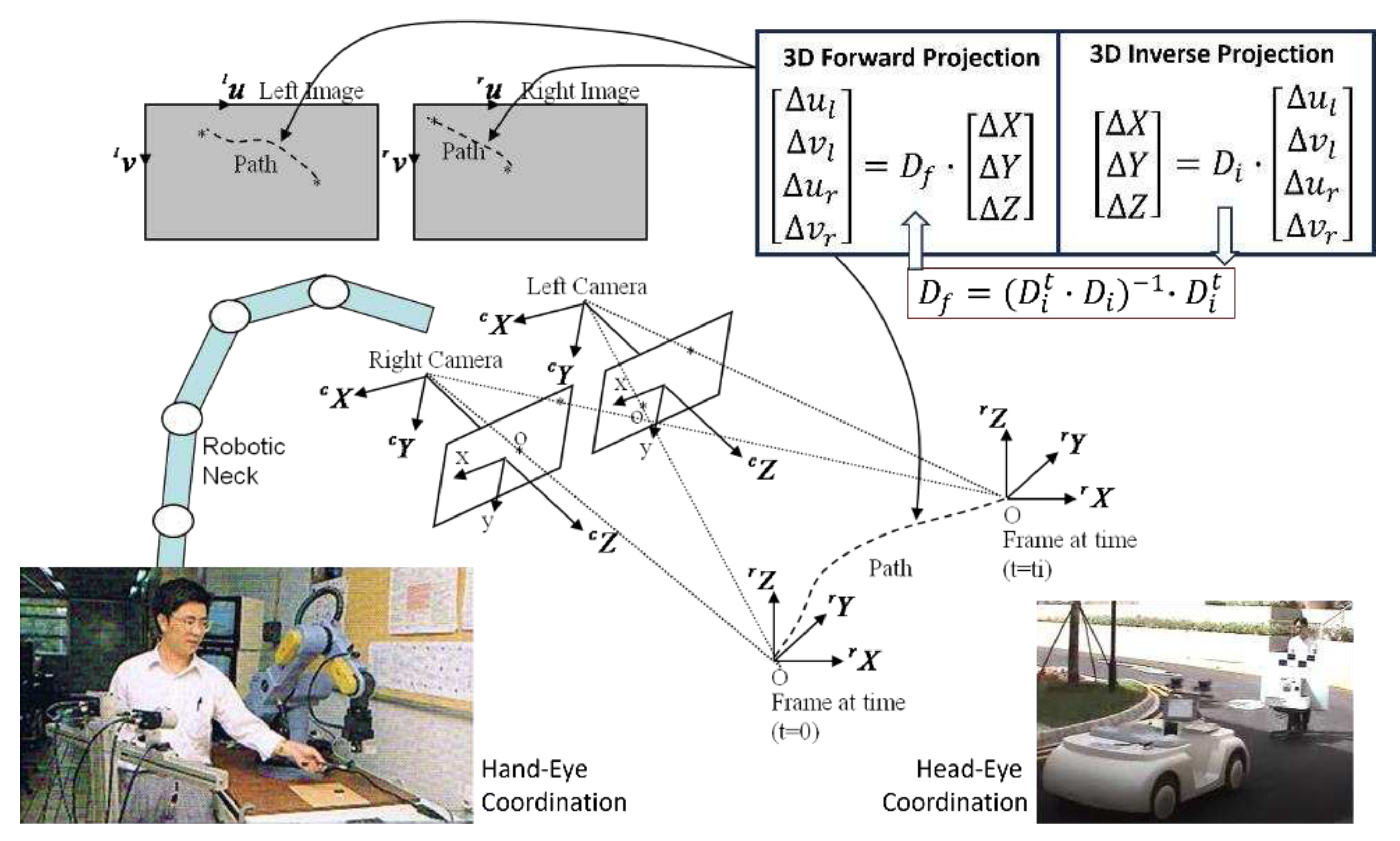
In summary, Equation 22 and Equation 23 fully describe 3D forward and inverse projections of displacement in a binocular vision system. These two solutions are iterative in nature and could be used inside the outer loop of perception, planning and control of autonomous robots as shown in Figure 7.

Especially, Equation 22 enables autonomous robots to achieve human-like hand-eye coordination and head-eye coordination as shown in Figure 7. For example, a control task of hand-eye coordination or head-eye coordination could be defined as the goal which is to minimize error vector

{(∆ u_{l}, ∆ v_{l}, ∆ u_{r}, ∆ v_{r})}^{t}

. As illustrated in Figure 7, the history of error vector

{(∆ u_{l}, ∆ v_{l}, ∆ u_{r}, ∆ v_{r})}^{t}

will appear as paths which could be observed inside both left and right images.

5. Experimental Results

The first important contribution of this paper is the result which is summarized by Figure 6. The second important contribution from this paper is the result outlined in Figure 7. In this section, we will share two experiments which validate the results shown in Figure 6 and Figure 7, respectively.

5.1. Real Experiment Validating Equation of 3D Inverse Projection of Position

Here, we would like to share an experiment which makes use of low-cost hardware with low-resolution binocular cameras and a small-sized checkerboard. In this way, we could appreciate the validity of Equation 20 and the result summarized in Figure 6.

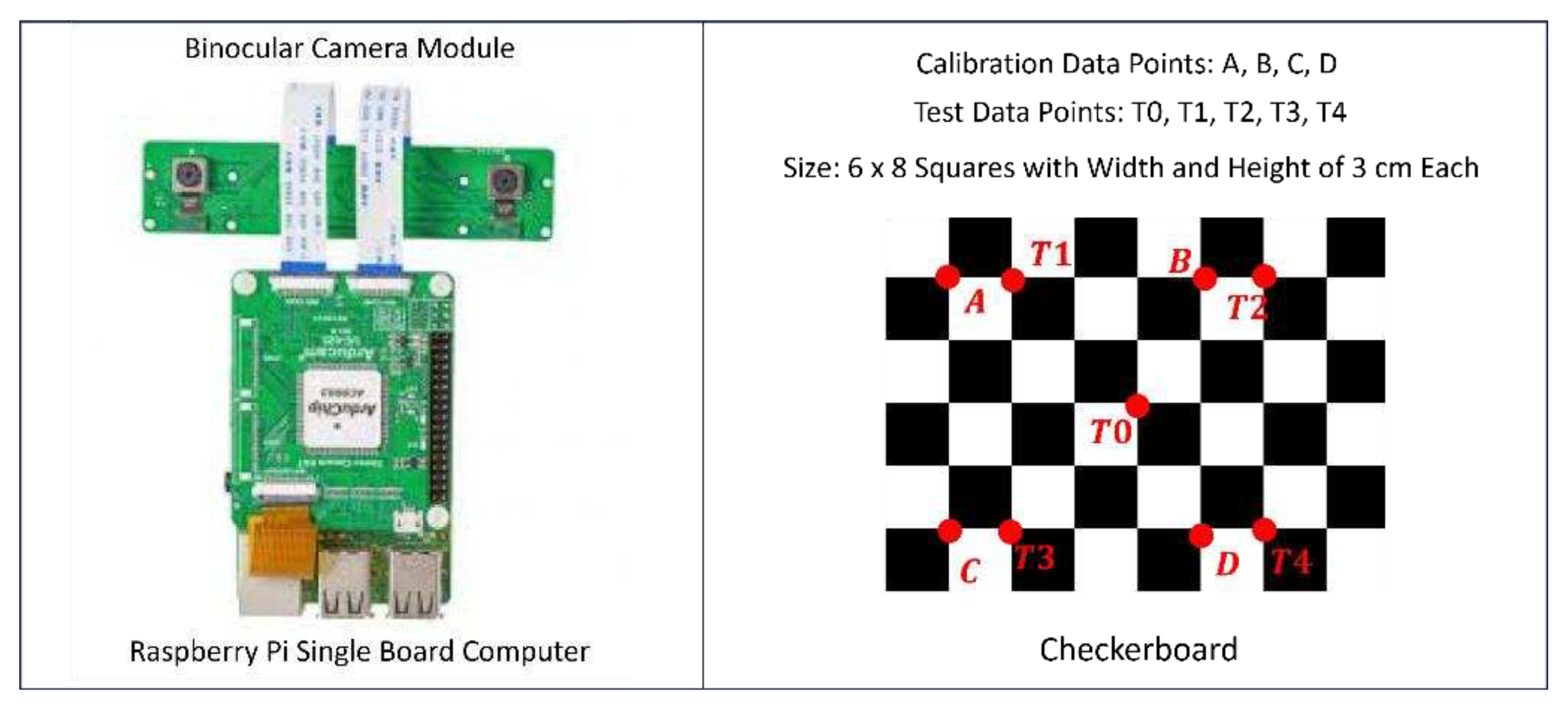
As shown in Figure 8, the experimental hardware includes a Raspberry Pi single board computer, a binocular vision module, and a checkerboard. The image resolution of the binocular cameras is

480 \times 320

pixels. The checkerboard has the size of

18 \times 24

cm, which is divided into

6 \times 8

squares with the size of

3.0 \times 3.0

cm each.

Inside the checkerboard,

{A, B, C, D}

serve as calibration data-points for the purpose of determining matrix

B_{i}

in Equation 20, while

{T_{0}, T_{1}, T_{2}, T_{3}, T_{4}}

serve as test data-points of the calibration result (i.e., to test the validity of matrix

B_{i}

in Equation 20).

Refer to Equation 20, matrix

B_{i}

is a

4 \times 5

matrix in which there are nineteen independent elements or parameters. Since a single Equation 20 will impose three constraints, at least seven pairs of

{X, Y, Z}

and

{u_{l}, v_{l}, u_{r}, v_{r}}

are needed for us to fully determine matrix

B_{i}

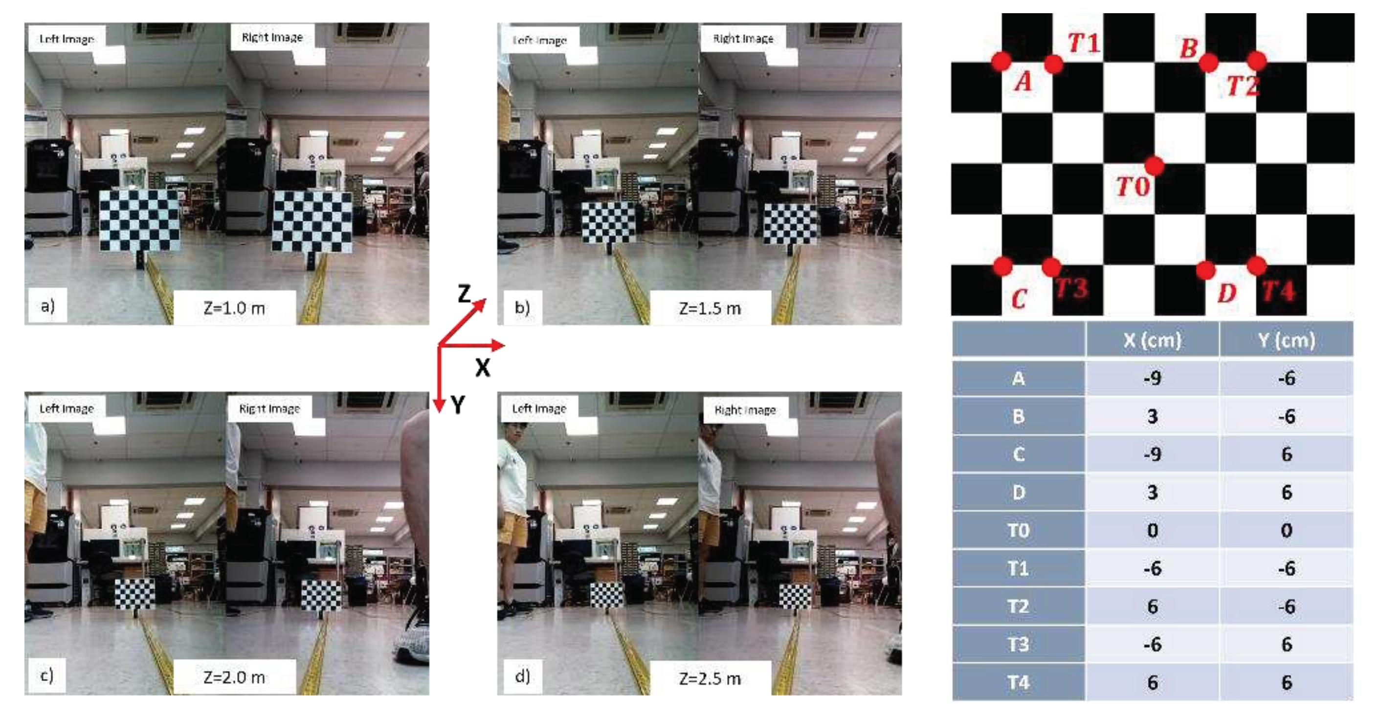
As shown in Figure 9, we define a reference coordinate system as follows: Its Z axis is parallel to the ground and is pointing toward the scene. Its Y axis is perpendicular to the ground and is pointing downward. Its X axis is pointing toward the right-hand side.

Then, we place the checkerboard at four locations in front of the binocular vision system. The Z coordinates of these four locations are 1.0 m, 1.5 m, 2.0 m, and 2.5 m, respectively. The checkerboard is perpendicular to Z axis, which passes through test data-point

T_{0}

. Therefore, the X and Y coordinates of the calibration data-points

{A, B, C, D}

and the test data-points

{T_{0}, T_{1}, T_{2}, T_{3}, T_{4}}

are known in advance. The values of these X and Y coordinates are shown inside Figure 9.

When the checkerboard is placed at one of the above-mentioned four locations, a pair of stereo images is taken. The index coordinates of the calibration data-points and the test data-points could be determined either automatically or manually.

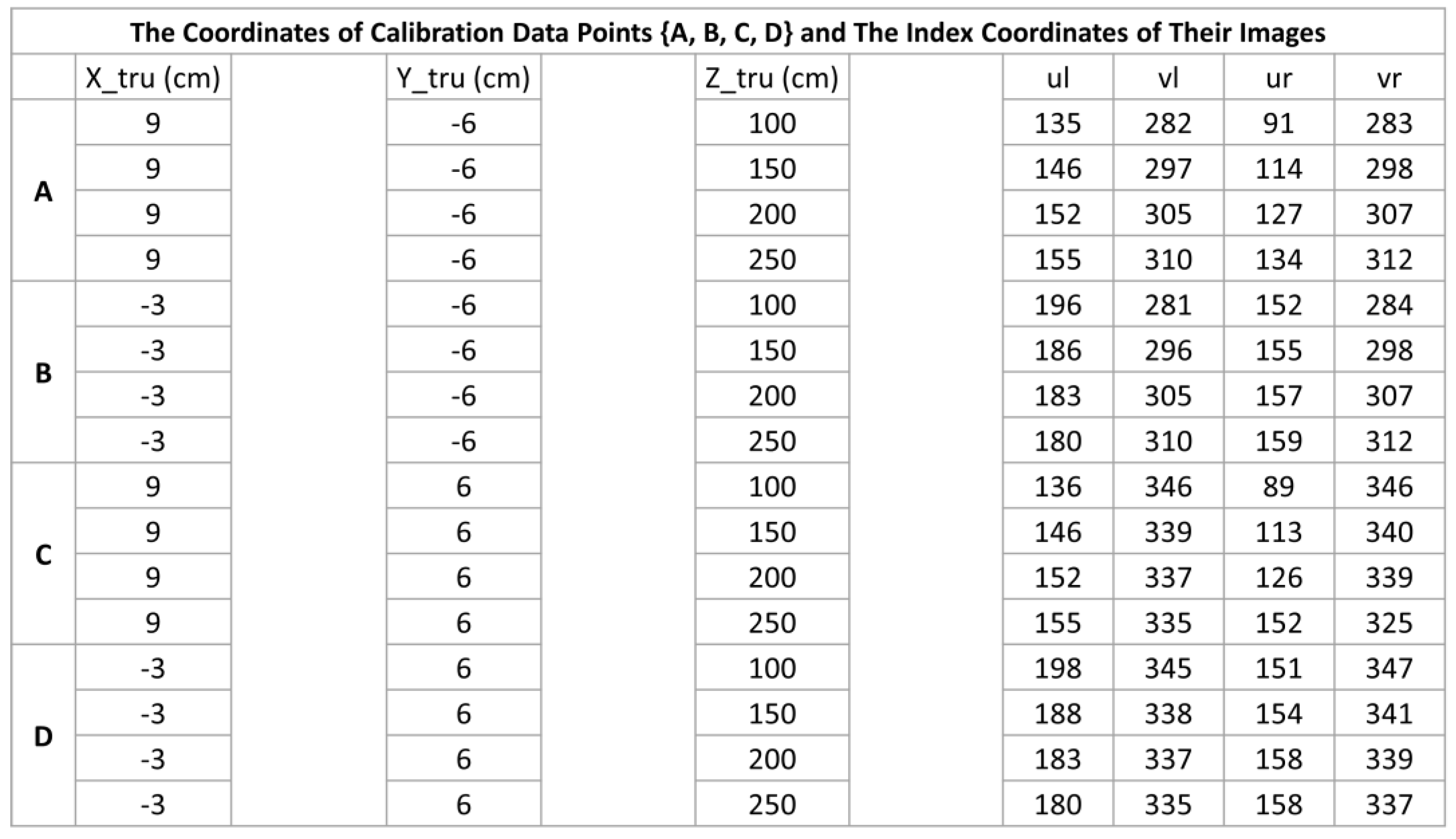
By putting the 3D coordinates and index coordinates of the calibration data-points together, we obtain Table 1 which contains the data needed for calibrating the equation of 3D inverse projection of binocular vision (i.e., Equation 20).

With the use of data listed in Table 1, we obtain the following result of matrix

B_{i}

B_{i} = [\begin{matrix} - 0.4251 & - 0.7861 & \begin{matrix} - 0.2245 & 0.8267 & 92.6220 \end{matrix} \\ 0.2167 & - 0.3717 & \begin{matrix} - 0.2730 & 0.9845 & - 196.0451 \end{matrix} \\ \begin{matrix} - 1.5409 \\ - 0.0874 \end{matrix} & \begin{matrix} 14.4961 \\ 0.1758 \end{matrix} & \begin{matrix} \begin{matrix} 1.2774 \\ 0.0873 \end{matrix} & \begin{matrix} - 14.9300 \\ - 0.1758 \end{matrix} & \begin{matrix} - 71.2214 \\ 1.0000 \end{matrix} \end{matrix} \end{matrix}]

(24)

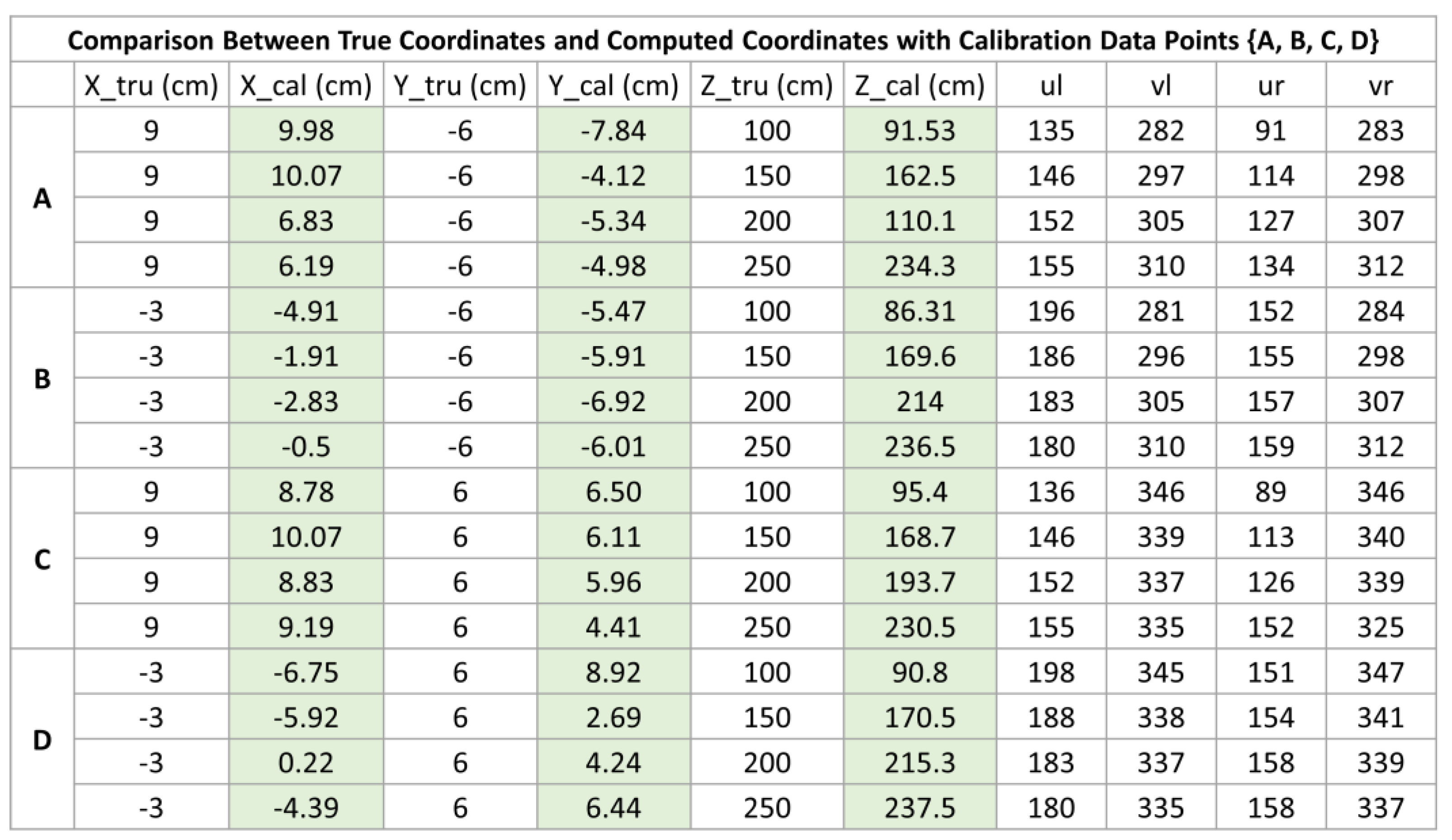
Now, we use the index coordinates in Table 1, calibrated matrix

B_{i}

, and Equation 20 to calculate the 3D coordinates of calibration data-points

{A, B, C, D}

. By putting these calculated 3D coordinates into Table 1, we will obtain Table 2 which helps us to compare between the true values of

\{A, B, C, D\}

’s 3D coordinates and the calculated values of

{A, B, C, D}

’s 3D coordinates.

Similarly, we use the index coordinates of the test data-points

{T_{0}, T_{1}, T_{2}, T_{3}, T_{4}}

, calibrated matrix

B_{i}

, and Equation 20 to calculate the 3D coordinates of

{T_{0}, T_{1}, T_{2}, T_{3}, T_{4}}

. Then, by putting the true values of

{T_{0}, T_{1}, T_{2}, T_{3}, T_{4}}

’s 3D coordinates and the calculated values of

{T_{0}, T_{1}, T_{2}, T_{3}, T_{4}}

’s 3D coordinates, we obtain Table 3 which helps us to appreciate the usefulness and validity of Equation 20.

In view of the low-resolution of digital images (i.e.,

480 \times 320

pixels) and a small-sized checkerboard (i.e.,

18 \times 24

cm divided into

6 \times 8

squares), we could say that the comparison results shown in Table 2 and Table 3 are reasonably good enough for us to experimentally validate Equation 20. In practice, images with much higher resolutions and checkerboards of larger sizes will naturally increase the accuracy of binocular vision calibration as well as the accuracy of calculated 3D coordinates by using Equation 20.

5.2. Simulation Validating Equation of 3D Inverse Projection of Displacement

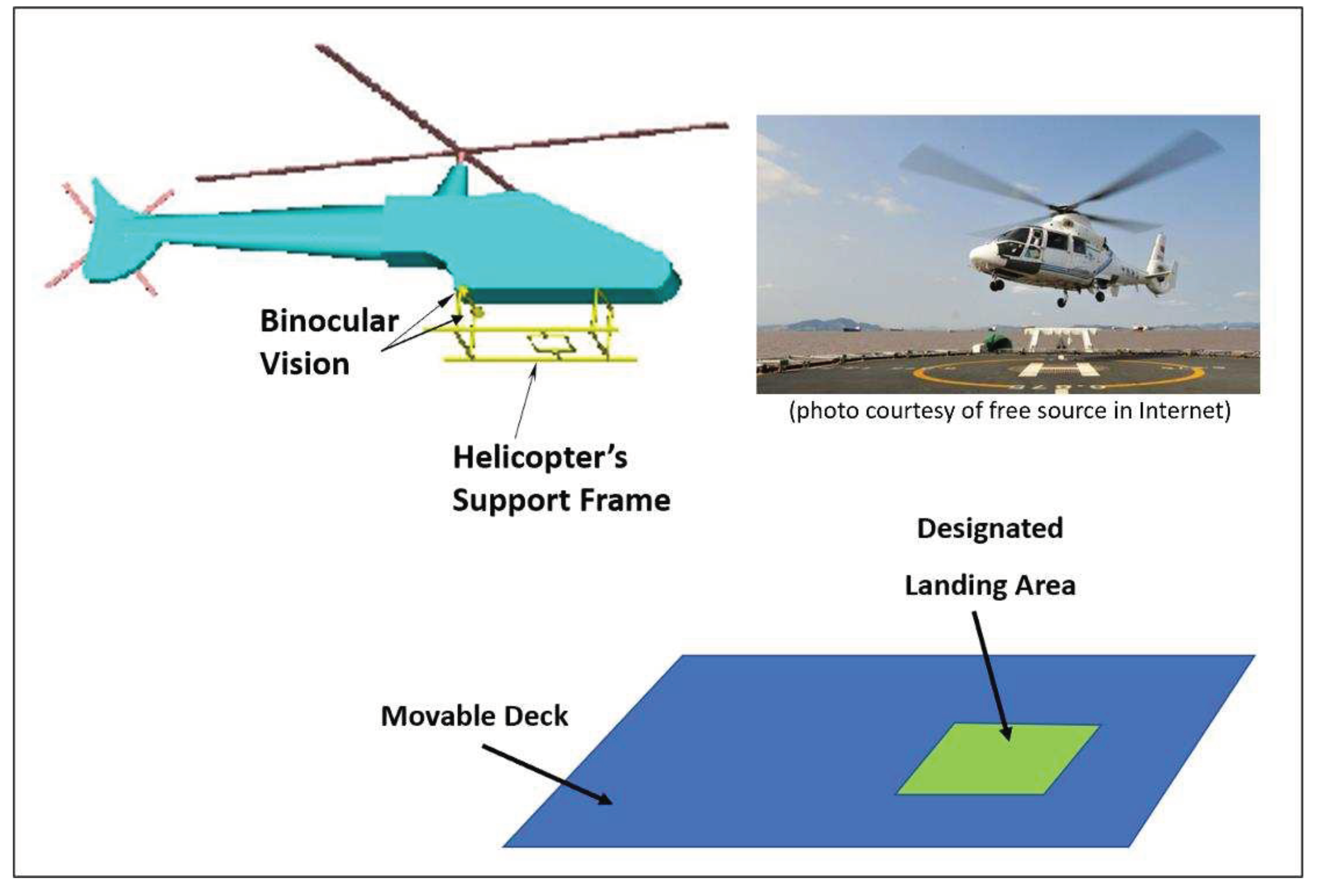
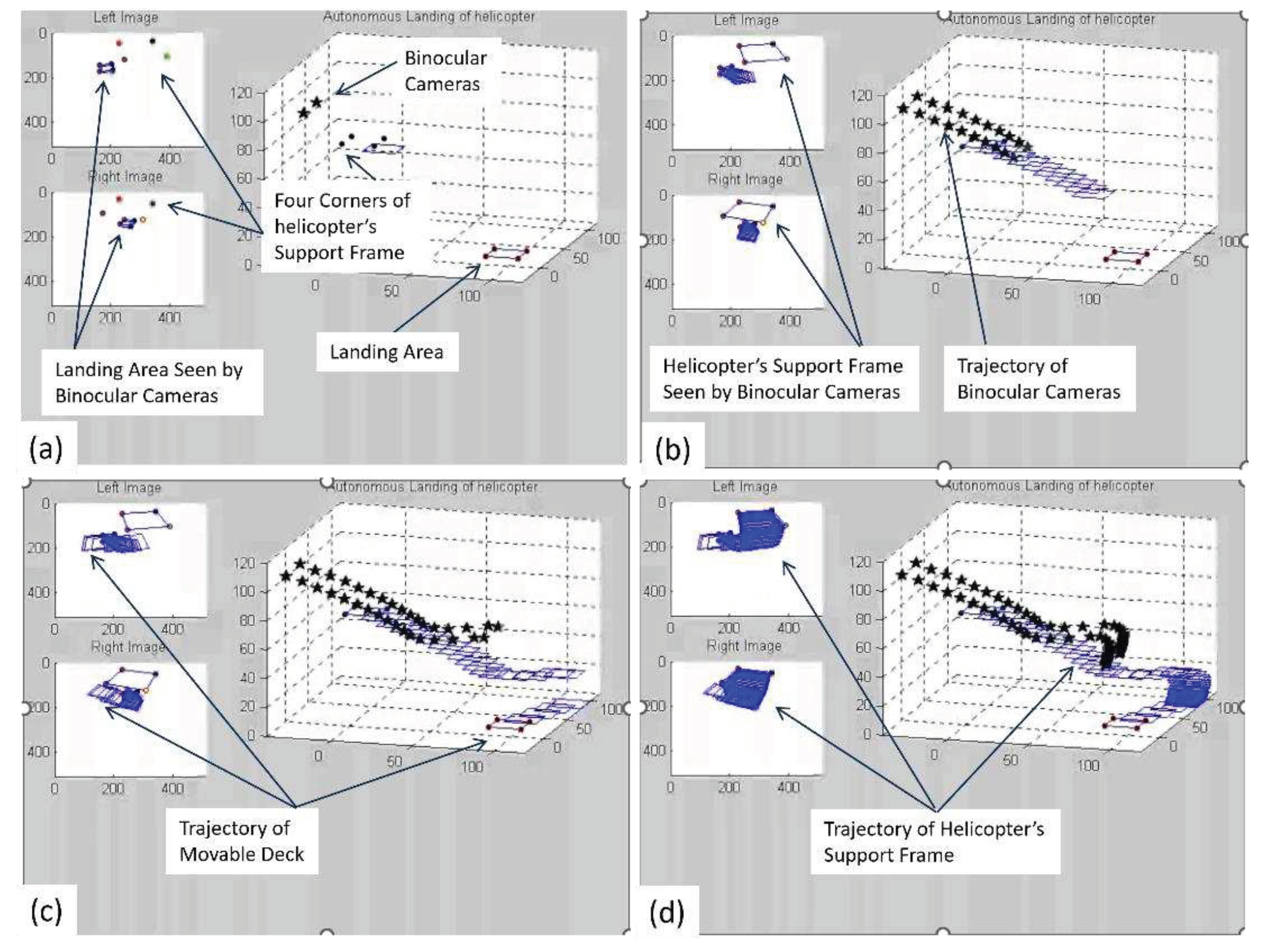
The picture of hand-eye coordination shown inside Figure 7 was a real experiment which has demonstrated the validity of the 3D inverse projection of displacement in binocular vision, as described by Equation 22. The video of real demonstration has been broadcasted during a national TV news in Singapore. Here, we would like to share a simulation result under the context of head-eye coordination which guides a helicopter to land on a ship’s movable deck, as illustrated by Figure 10.

In Equation 22, matrix

D_{i}

is a

3 \times 4

matrix which has eleven independent elements or parameters. Since one pair of

\{∆ X . ∆ Y, ∆ Z\}}

and {

∆ u_{l}, ∆ v_{l}, ∆ u_{r}, ∆ v_{l}}

imposes three constraints, four pairs of such calibration data sets are enough to fully determine matrix

D_{i}

After calibration, Equation 22 could be used to serve as the perception and planning modules as shown in Figure 2. The simulation result of Figure 10’s scenario is shown in Figure 11. The full video could be viewed at https://youtu.be/BCWpOJyGr6E

It is interesting to take note that under the context of a binocular vision system mounted inside the head of an autonomous humanoid robot, a pair of human-like robot hands will automatically generate five pairs of

\{∆ X . ∆ Y, ∆ Z\}}

and {

∆ u_{l}, ∆ v_{l}, ∆ u_{r}, ∆ v_{l}}

which correspond to the displacements among the five pairs of fingertips. Such observation helps us to understand the power and flexibility of human beings’ binocular vision.

6. Conclusions

In this paper, we have proven two important equations, which are Equation 20 and Equation 22. These two equations fully describe the 3D projections in a human-like binocular vision system. It is interesting to know that they are like the equations underlying 2D forward and inverse projections in a monocular vision system. These findings help us to unify the geometrical aspects of monocular vision and binocular vision in terms of equations for forward and inverse projections. Most importantly, Equation 20 and Equation 22 are in the form of two systems of linear equations, which could be easily implemented by a network of artificial neurons. Therefore, these theoretical findings from this paper help us to understand why a huge quantity of visual signals from human vision will not cause fatigue to human beings’ brains. In addition, the matrices in Equation 20 and Equation 22 could be easily obtained by a calibration process without the need of knowing the intrinsic parameters of the cameras in binocular vision. Interestingly, if a binocular vision system is mounted inside the head of a humanoid robot, the fingertips of the humanoid robot will be able to readily provide the necessary datasets for the calibration of both Equation 20 and Equation 22. This implies that periodic calibration on the fly or on the go is not a difficult issue. This fact helps us to understand why human vision could adapt to the growth of human being’s body. We hope to see wide adoption and application of Equation 20 and Equation 22 in our future research and product development, which are related to the use of binocular vision for various purposes in science, engineering and industry.

Author Contributions

Conceptualization, Ming Xie; methodology, Ming Xie and Yuhui Fang; software, Yuhui Fang and Tingfeng Lai; validation, Yuhui Fang and Tingfeng Lai; formal analysis, Ming Xie; investigation, Ming Xie, Yuhui Fang and Tingfeng Lai; resources, Ming Xie; data curation, Yuhui Fang; writing—original draft preparation, Ming Xie; writing—review and editing, Ming Xie.; visualization, Ming Xie and Yuhui Fang; supervision, Ming Xie; project administration, Ming Xie; funding acquisition, Ming Xie. All authors have read and agreed to the published version of the manuscript.

Funding

This research was funded by the Future Systems and Technology Directorate, Ministry of Defense, Singapore, grant number PA9022201473”.

Institutional Review Board Statement

Not applicable”.

Data Availability Statement

All data related to this paper will be made available upon request. The access to the data is subject to the data protection policy of Nanyang Technological University, Singapore.

Acknowledgments

We would like to acknowledge the financial support from the Future Systems and Technology Directorate, Ministry of Defense, Singapore, to NTU’s RobotX Challenge team.

Conflicts of Interest

There is no conflict of interest.

References

Xie, M. Hu, Z. C. and Chen, H. New Foundation of Artificial Intelligence. World Scientific, 2021.
Horn, B. K. P. Robot Vision. The MIT Press, 1986.
Tolhurst, D. J. Sustained and transient channels in human vision. Vision Research, 1975; Volume 15, Issue 10, pp1151-1155. [CrossRef]
Fahle M and Poggio T. Visual hyperacuity: spatiotemporal interpolation in human vision, Proceedings of Royal Society, London, 1981. [CrossRef]
Enns, J. T. and Lleras, A. What’s next? New evidence for prediction in human vision. Trends in Cognitive Science, 2008; Volume 12, Issue 9, pp327-333.
Laha, B., Stafford, B. K. and Huberman, A. D. Regenerating optic pathways from the eye to the brain. Science, 2017; Volume 356, Issue 6342, pp1031-1034. [CrossRef]
Gregory, R. Eye and Brain: The Psychology of Seeing - Fifth Edition, The Princeton University Press, 2015.
Pugh, A. (editor). Robot Vision. Springer-Verlag, 2013.
Samani, H. (editor). Cognitive Robotics. CRC Press, 2015.
Erlhagen, W. and Bicho, E. The dynamic neural field approach to cognitive robotics. Journal of Neural Engineering, 2006; Volume 3, Number 3. [CrossRef]
Cangelosi, A. and Asada, M. Cognitive Robotics. The MIT Press, 2022.
Faugeras, O. Three-dimensional Computer Vision: A Geometric Viewpoint. The MIT Press, 1993.
Paragios, N., Chen, Y. M. and Faugeras, O. (editors). Handbook of Mathematical Models in Computer Vision. Springer, 2006.
Faugeras, O., Luong, Q. T. and Maybank, S. J. Camera self-calibration: Theory and experiments. European Conference on Computer Vision. Springer, 1992; LNCS, Volume 588. [CrossRef]
Stockman, G. and Shapiro, L. G. Computer Vision. Prentice Hall, 2001.
Shirai, Y. Three-Dimensional Computer Vision. Springer, 2012.
Khan, S., Rahmani, H., Shah, S. A. A. and Bennamoun, M. A Guide to Convolutional Neural Networks for Computer Vision. Springer, 2018. [CrossRef]
Szeliski, R. Computer Vision: Algorithms and Applications. Springer, 2022.
Brooks, R. New Approaches to Robotics. Science, 1991; Volume 253, Issue 5025. [CrossRef]
Xie, M. Fundamentals of Robotics: Linking Perception to Action. World Scientific, 2003.
Siciliano, B. and Khatib, O. Springer Handbook of Robotics. Springer, 2016.
Murphy, R. Introduction to AI Robotics - Second Edition. The MIT Press, 2019.

Figure 1. Comparison of the motion aspects between human eye and electronic camera (photo courtesy of free source in Internet).

Figure 2. Outer loop of perception, planning and control inside autonomous robot arm manipulator and autonomous car-like robot.

Figure 3. Two fundamental questions faced by a human-like binocular vision system are: a) what have been seen? and where are the entities seen?

Figure 4. A single camera is the basis of a monocular vision.

Figure 5. Full illustration of a monocular vision system’s 2D forward and inverse projections.

Figure 6. Full illustration of a binocular vision system’s 3D forward and inverse projections.

Figure 7. Scenarios of achieving human-like hand-eye coordination and head-eye coordination.

Figure 8. Experimental hardware includes Raspberry Pi single board computer with a binocular vision module and a checkerboard which serves as input of calibration data-points as well as test data-points.

Figure 9. Data set for calibrating matrix

B_{i}

in Equation 20.

Figure 9. Data set for calibrating matrix

B_{i}

in Equation 20.

Figure 10. Illustration of head-eye coordination for the guidance of helicopter during the landing on a ship’s movable deck.

Figure 11. Simulation result of using Equation 22 to serve as perception and planning modules under the context of head-eye coordination for the guidance of helicopter landing on movable deck.

Table 1. 3D coordinates and Index coordinates of data-points for calibrating binocular vision.

Table 2. Comparison between true values and calculated values of calibration data-points

\{A, B, C, D\}

’s 3D coordinates.

Table 2. Comparison between true values and calculated values of calibration data-points

\{A, B, C, D\}

’s 3D coordinates.

Table 3. Comparison between true values and calculated values of test data-points

{T_{0}, T_{1}, T_{2}, T_{3}, T_{4}}

’s 3D coordinates.

Table 3. Comparison between true values and calculated values of test data-points

{T_{0}, T_{1}, T_{2}, T_{3}, T_{4}}

’s 3D coordinates.

Disclaimer/Publisher’s Note: The statements, opinions and data contained in all publications are solely those of the individual author(s) and contributor(s) and not of MDPI and/or the editor(s). MDPI and/or the editor(s) disclaim responsibility for any injury to people or property resulting from any ideas, methods, instructions or products referred to in the content.

© 2023 by the authors. Licensee MDPI, Basel, Switzerland. This article is an open access article distributed under the terms and conditions of the Creative Commons Attribution (CC BY) license (http://creativecommons.org/licenses/by/4.0/).

Copyright: This open access article is published under a Creative Commons CC BY 4.0 license, which permit the free download, distribution, and reuse, provided that the author and preprint are cited in any reuse.

MDPI Initiatives

Important Links

Choose an area of interest and we will send you notifications of new preprints at your preferred frequency.

Disclaimer

New Solution to 3D Projection in Human-like Binocular Vision

Abstract

1. Introduction

2. Problem Statement

3. Related Works

3.1. Concept of Kinematic Chain

3.2. Forward Projection Matrix of Camera

3.3. 3D Forward Projection of Monocular Vision

3.4. 3D Inverse Projection of Monocular Vision

3.5. 2D Forward Projection of Monocular Vision

3.6. 2D Inverse Projection of Monocular Vision

3.7. Textbook Solution of Computing 3D Coordinates from Binocular Vision

4. Equations of 3D Projection in Human-like Binocular Vision

4.1. Equation of 3D Inverse Projection of Position in Binocular Vision

4.2. Equation of 3D Forward Projection of Position in Binocular Vision

4.3. Equation of 3D Inverse Projection of Displacement of Binocular Vision

4.4. Equation of 3D Forward Projection of Displacement of Binocular Vision

5. Experimental Results

5.1. Real Experiment Validating Equation of 3D Inverse Projection of Position

5.2. Simulation Validating Equation of 3D Inverse Projection of Displacement

6. Conclusions

Author Contributions

Funding

Institutional Review Board Statement

Data Availability Statement

Acknowledgments

Conflicts of Interest

References

MDPI Initiatives

Important Links

Subscribe