New Solution to 3D Projection in Human-like Binocular Vision

1. Introduction

We are living inside an ocean of signals. Among all the signals, the most important ones should be the visual signals. Therefore, vision is extremely important to the intelligence of human beings [1]. Similarly, vision is also extremely important to the intelligence of autonomous robots [2]. In the past decades, there have been extensive research activities dedicated to computer vision research. The intensity of such research has been witnessed by the huge number of conference paper submissions to ICCV (i.e., International Conference on Computer Vision) and CVPR (i.e., International Conference of Computer Vision and Pattern Recognition). However, despite the continuous efforts of research, today’s computer vision is far behind the performance of human vision. Hence, it is important for us to seriously analyze the gaps between computer vision and human vision.

As shown in Figure 1, the motion aspects of a human eye are like a PTZ camera. Here, PTZ stands for pan, tilt and zoom. We know that a human eye can undertake continuous motion and zooming. This implies that a human eye has an infinite number of PTZ parameters (i.e., the coefficients of pan, tilt and zoom). However, our vision processes are not sensitive to the change of PTZ parameters [3,4,5].

It is true to say that one could employ multiple pairs of binocular vision systems which have different sets of focal lengths. However, such solution has many limitations in size, flexibility, performance, and hardware cost. Electronic solution of undertaking zooming by a camera should be the future trend.

On the other hand, a human eye has about 120 million rod cells and 6 million cone cells. These cells are responsible for converting lights into visual signals which will then be processed by a human’s brain. Our daily experience tells us that our brains do not experience any heating-effect and fatigue despite the huge quantity of visual signals under processing in real-time and continuously. This observation leads us to believe that the formulas of the visual processes running inside a human brain must be simple and be suitable for easy and quick learning by human-brain-like neural systems [6,7].

Figure 1. Comparison of the motion aspects between human eye and electronic camera (photo courtesy of free source in Internet).

Figure 1. Comparison of the motion aspects between human eye and electronic camera (photo courtesy of free source in Internet).

Inspired by the above concise analysis, it is reasonable for us to believe that future research direction in computer vision (or robot vision) should be focused on the discovery and invention of the principles and algorithms which are like the formulas behind the visual processes running inside a human brain. Hopefully, the outcomes of this discovery and invention could be implemented in a brain-like digital computer [7].

In this paper, we prove and validate a new solution which will enable autonomous robots, such as car-like robots and humanoid robots, to undertake 3D projection in a human-like binocular vision. The 3D projection includes both forward and inverse projections among positions as well as displacements. This work is inspired by human beings’ visual perception systems which could easily handle huge amount of inflow visual signals without causing fatigues to human brains.

This paper is organized as follows: The technical problem under investigation will be described in Section 2. The background knowledge or related works will be presented in Section 3. The new solution to 3D projection in a human-like binocular vision and its proof will be shown in Section 4. Experimental results for validating the described new solution are included in Section 5. Finally, we conclude this paper in Section 6.

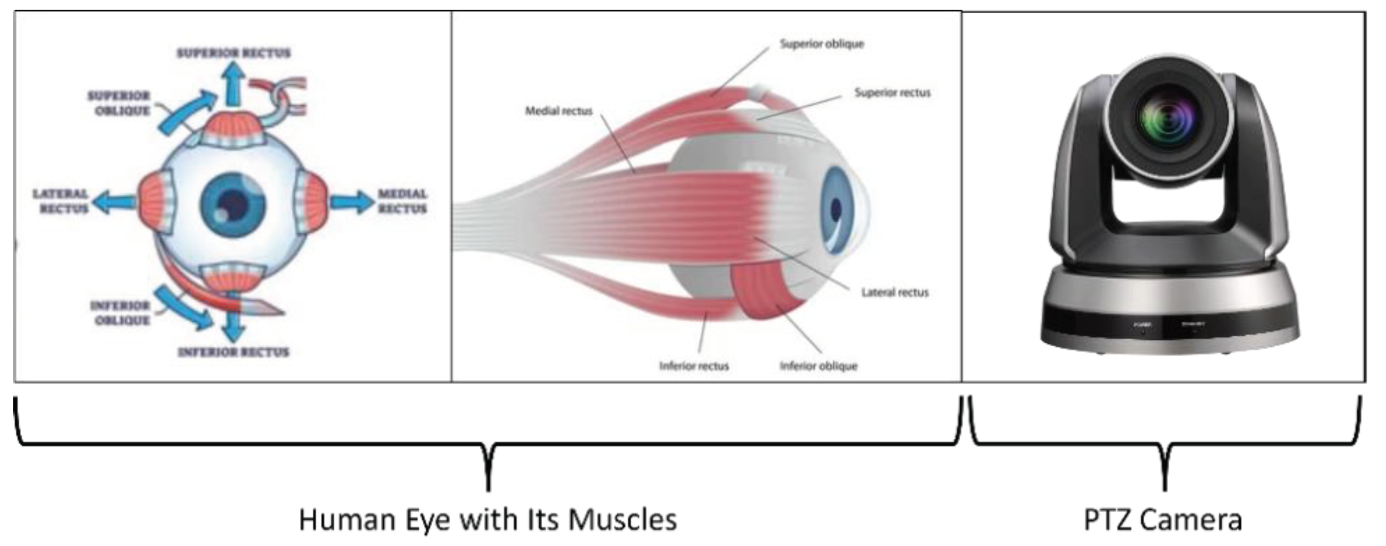
2. Problem Statement

We are living in a three-dimensional space or scene. Similarly, an autonomous robot also manifests its existence or activities in a three-dimensional space or scene. In general, a 3D scene consists of a set of entities which have both global poses (i.e., positions and orientations) and local shapes. If we follow the convention in robotics, each entity in a scene will be assigned a coordinate system (or frame in short) which is called a local coordinate system (or local frame in short). Within a global coordinate system (or global frame in short), an entity’s pose is represented by the position and orientation of its local coordinate system. Within the local coordinate system of an entity, the shape of the entity could be represented by a mesh of triangles or a cloud of points [8].

Therefore, the success of our daily behaviors or activities depends on our mental capabilities of perceiving a three-dimensional space or scene. Similarly, the success of an autonomous robot also depends on its mental capabilities of perceiving a three-dimensional space or scene. More specifically, the intelligence of a human being or an autonomous robot depends on the proper functioning of the outer loop which includes perception, planning and control as shown in Figure 2 [9,10].

It goes without saying that human vision is binocular in nature. Certainly, binocular vision has empowered a human’s mind to achieve impressive intelligent behaviors guided by the perception-planning-control loop. Hence, there is no doubt to us that it is an important research topic which aims at achieving human-like intelligent behaviors by autonomous robots under the guidance of human-like binocular vision [11].

Figure 2. Outer loop of perception, planning and control inside autonomous robot arm manipulator and autonomous humanoid robot.

Figure 2. Outer loop of perception, planning and control inside autonomous robot arm manipulator and autonomous humanoid robot.

With visual signals as input, two important tasks of binocular vision are to provide information and knowledge about the answers to these two general questions which are: a) what has been seen? and b) where are the entities seen? Figure 3 illustrates these two related questions faced by a binocular vision system. Please take note that a third popular question in binocular vision is: what are the shapes of the entities seen? However, the solution to the first question is also the solution to this third question. Hence, without loss of generality, it is not necessary to specifically highlight this third popular question.

As shown in Figure 3, the first question refers to the problem of entity detection (e.g., object detection), entity identification (e.g., object identification), or entity classification (e.g., object classification). The second question refers to the problem of 2D/3D localization or 2D/3D reconstruction. In this paper, the problem under investigation is to develop a better solution which provides the answer to the second question.

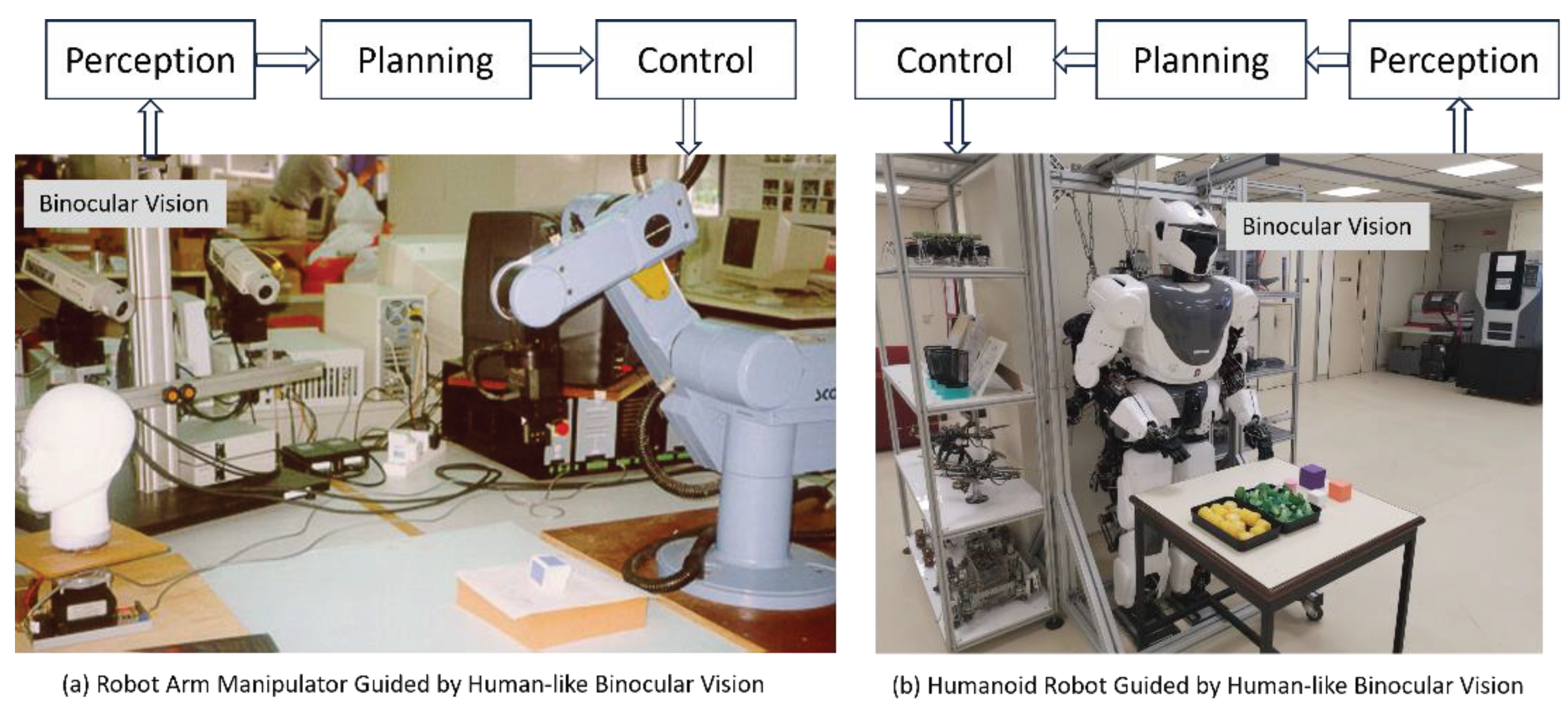
3. Related Works

The problem under investigation in this paper is about how to do 3D projection in a human-like binocular vision system which does not require both expensive and extensive computations. This paper is not discussing about camera calibration. Obviously, the topic under discussion in this paper belongs to computer vision. which is a well-established discipline in science and engineering [12,13,14,15,16,17,18]. Since computer vision is a very important module or perception system inside autonomous robots, the problem under investigation is also related to robotics, in which an interesting topic is about forward and inverse kinematics. In this section, we summarize the background knowledge (or related works) in robotics and computer vision, which serve as the foundation behind the proof of the new solution presented in this paper. The related works presented in this section also serve as the necessary proofing steps toward the important new theoretical result of this paper.

3.1. Concept of Kinematic Chain

In robotics [19,20,21,22], the study of kinematics starts with the assignment of a local coordinate system (or frame) to each rigid body (e.g., a link in a robot). In this way, a series of links in a robot arm manipulator become a kinematic chain. Hence, the topic of kinematics in robotics is about the study the motion relationships among the local coordinate systems assigned to the links of a robot arm manipulator.

In general, a vision system must involve the use of at least one camera which includes a lens (i.e. a rigid body), an imaging sensor array (i.e. a rigid body) and a digital image matrix (i.e. a virtual rigid body). Also, a camera must be mounted on a robot, a machine, or a supporting ground, each of which could be considered as a rigid body. Hence, a camera should be considered as a kinematic chain. In this way, we could talk about the kinematics of a camera, a monocular vision, or a binocular vision.

For example, in Figure 3, a binocular vision system could be considered as the sum of two monocular vision systems. Each monocular vision system consists of a single camera. If we look at the left camera, we could see its kinematic chain which includes the motion transformations such as: transformation from world frame to left-camera frame, transformation from left-camera frame to analogue-image frame, and transformation from analogue-image frame to digital-image frame.

3.2. Forward Projection Matrix of Camera

A single camera is the basis of a monocular vision. Before we could understand the 2D forward and inverse projections of monocular vision, it is necessary for us to know the details of a camera’s forward projection matrix.

Refer to Figure 4. With the use of the terminology of kinematic chain, the derivation of camera matrix starts with the transformation from reference frame to camera frame. If the coordinates of point Q with respect to reference frame are $(X,Y,Z)$, the coordinates $(X_c,Y_c,Z_c)$ of the same point Q with respect to camera frame will be [12]:

$$\left[\begin{array}{c}{X}_c\\ Y_c\\ \begin{array}{c}{Z}_c\\ 1\end{array}\end{array}\right]=\left[\begin{array}{ccc}{r}_{11}& r_{12}& \begin{array}{cc}{r}_{13}& t_x\end{array}\\ r_{21}& r_{22}& \begin{array}{cc}{r}_{23}& t_y\end{array}\\ \begin{array}{c}{r}_{31}\\ 0\end{array}& \begin{array}{c}{r}_{32}\\ 0\end{array}& \begin{array}{cc}\begin{array}{c}{r}_{33}\\ 0\end{array}& \begin{array}{c}{t}_z\\ 1\end{array}\end{array}\end{array}\right]\bullet \left[\begin{array}{c}X\\ Y\\ \begin{array}{c}Z\\ 1\end{array}\end{array}\right]$$

(1)

where rotation matrix $\{r_{ij},i\in \left[\mathrm{1,3}\right],j\in [\mathrm{1,3}\left]\right\}$ represents the orientation of reference frame with respect to camera frame, and translation vector ${(t_x,t_y,t_z)}^t$ represents the position of reference frame’s origin with respect to camera frame.

Inside the camera frame, the transformation from the coordinates $(X_c,Y_c,Z_c)$ of point Q to the analogue image coordinates ${(x,y)}^t$ of point q will be:

$$\left[\begin{array}{c}s\bullet x\\ s\bullet y\\ s\end{array}\right]=\left[\begin{array}{ccc}f& 0& \begin{array}{cc}0& 0\end{array}\\ 0& f& \begin{array}{cc}0& 0\end{array}\\ 0& 0& \begin{array}{cc}1& 0\end{array}\end{array}\right]\bullet \left[\begin{array}{c}{X}_c\\ Y_c\\ \begin{array}{c}{Z}_c\\ 1\end{array}\end{array}\right]$$

(2)

where $f$ is the focal length of the camera and $s$ is a scaling factor.

By default, we are using digital cameras. Hence, an analogue image is converted into its corresponding digital image. Such process of digitization results in the further transformation from analogue image frame to digital image frame. This transformation is described by the following equation:

$$\left[\begin{array}{c}s\bullet u\\ s\bullet v\\ s\end{array}\right]=\left[\begin{array}{ccc}\frac{1}{∆u}& 0& u_0\\ 0& \frac{1}{∆v}& v_0\\ 0& 0& 1\end{array}\right]\bullet \left[\begin{array}{c}s\bullet x\\ s\bullet y\\ s\end{array}\right]$$

(3)

where ${(u,v)}^t$ are the digital image coordinates of point q, $∆u$ is the width of a pixel (i.e., a digital image’s pixel density in horizontal direction), $∆v$ is the height of a pixel (i.e., a digital image’s pixel density in vertical direction), and ${(u_0,v_0)}^t$ are the digital image coordinates of the intersection point between the optical axis (i.e., camera frame’s Z axis) and the image plane (note: this point is also called a camera’s principal point).

Now, by substituting Equations (1) and (2) into Equation (3), we will be able to obtain the following equation [16]:

$$\left[\begin{array}{c}s\bullet u\\ s\bullet v\\ s\end{array}\right]=C_f\bullet \left[\begin{array}{c}X\\ Y\\ \begin{array}{c}Z\\ 1\end{array}\end{array}\right]$$

(4)

with

$$C_f=\left[\begin{array}{ccc}\frac{f}{∆u}& 0& \begin{array}{cc}{u}_0& 0\end{array}\\ 0& \frac{f}{∆v}& \begin{array}{cc}{v}_0& 0\end{array}\\ 0& 0& \begin{array}{cc}1& 0\end{array}\end{array}\right]\bullet \left[\begin{array}{ccc}{r}_{11}& r_{12}& \begin{array}{cc}{r}_{13}& t_x\end{array}\\ r_{21}& r_{22}& \begin{array}{cc}{r}_{23}& t_y\end{array}\\ \begin{array}{c}{r}_{31}\\ 0\end{array}& \begin{array}{c}{r}_{32}\\ 0\end{array}& \begin{array}{cc}\begin{array}{c}{r}_{33}\\ 0\end{array}& \begin{array}{c}{t}_z\\ 1\end{array}\end{array}\end{array}\right]$$

(5)

where matrix $C_f$ is called a camera’s forward projection matrix which is a $3\times 4$ matrix.

Figure 4. A single camera is the basis of a monocular vision.

Figure 4. A single camera is the basis of a monocular vision.

3.3. 3D Forward Projection of Monocular Vision

A monocular vision system uses a single camera. Its kinematic chain is the same as the one shown in Figure 4. Most importantly, Equation (4) describes 3D forward projection of a monocular vision system, in which 3D coordinates ${(X,Y,Z)}^t$ are projected into 2D digital image coordinates ${(u,v)}^t$.

3.4. 3D Inverse Projection of Monocular Vision

From the viewpoint of pure mathematics, Equation (4) could be re-written into the following form:

$$\left[\begin{array}{c}k\bullet X\\ k\bullet Y\\ \begin{array}{c}k\bullet Z\\ k\end{array}\end{array}\right]=C_i\bullet \left[\begin{array}{c}u\\ v\\ 1\end{array}\right]$$

(6)

with

$${C_i=(C_f^t\bullet C_f)}^{-1}\bullet C_f^t$$

(7)

and $k=1/s$. It is worth noting that Equation (6) has never been explicitly described in any textbook because it is useless in theory and in practice. However, Equation (6) has inspired us to derive Equation (20) which represents an important advance in computer vision, robot vision, and artificial intelligence.

In theory, Equation (6) describes 3D inverse projection of a monocular vision system. In practice, Equation (6) could be graphically represented by an artificial neural network which serves as predictor. The input layer consists of ${(u,v,1)}^t$ and the output layer consists of ${(X,Y,Z)}^t$. Matrix $C_i$ contains the weighting coefficients. Hence, it is clear to us that a different matrix $C_i$ will enable the prediction of coordinates ${(X,Y,Z)}^t$ on a different planar surface. Most importantly, matrix $C_i$ could be obtained by a top-down process of calibration or a bottom-up process of tuning (i.e., optimization). Therefore, Equation (6) serves as a good example which helps us to understand the difference between machine learning and machine calibration (or tuning).

Although $C_i$ is a $4\times 3$ matrix, it is not possible to use Equation (6) to generally compute 3D coordinates ${(X,Y,Z)}^t$ in an analogue scene from 2D index coordinates ${(u,v)}^t$ (i.e., u is column index while v is row index) in a digital image. However, the philosophy behind Equation (6) has inspired us to discover a similar, but very useful, 3D inverse projection of binocular vision which will be described in Section 4.

3.5. 2D Forward Projection of Monocular Vision

Refer to Figure 4. If we consider the points or locations on the OXY plane of reference frame, Z coordinate in Equation (4) becomes zero. Hence, Equation (4) could be re-written into the following form:

$$\left[\begin{array}{c}s\bullet u\\ s\bullet v\\ s\end{array}\right]=M_f\bullet \left[\begin{array}{c}X\\ Y\\ 1\end{array}\right]$$

(8)

where matrix $M_f$ is the version of matrix $C_f$ after removing its third column because Z is equal to zero. Clearly, matrix $M_f$ is a $2\times 2$ matrix and is invertible. As shown in Figure 8, Equation (8) describes the 2D forward projection from coordinates ${(X,Y)}^t$ on a plane of reference frame into digital image coordinates ${(u,v)}^t$ of monocular vision.

3.6. 2D Inverse Projection of Monocular Vision

Now, by inverting Equation (8), we could easily obtain the following result:

$$\left[\begin{array}{c}k\bullet X\\ k\bullet Y\\ k\end{array}\right]=M_i\bullet \left[\begin{array}{c}u\\ v\\ 1\end{array}\right]$$

(9)

with

$$M_i={(M_f^t\bullet M_f)}^{-1}\bullet M_f^t$$

(10)

where matrix $M_i$ is also a $2\times 2$ matrix.

It goes without saying that Equations (8) and (9) fully describe 2D forward and inverse projections of a monocular vision system as shown in Figure 5.

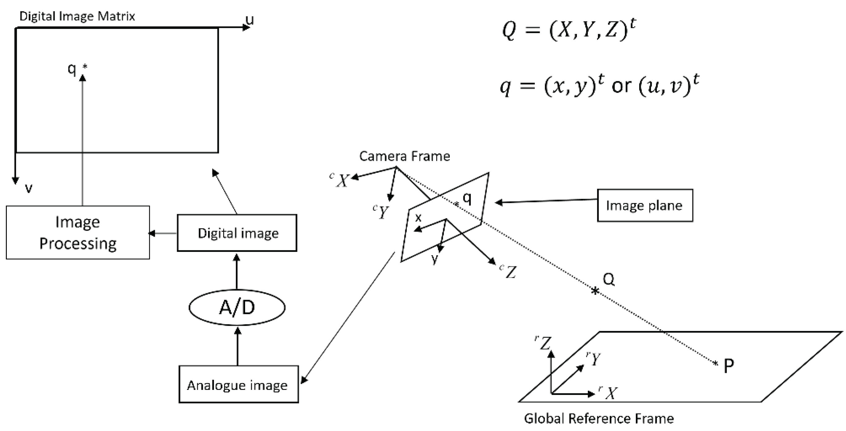
3.7. Textbook Solution of Computing 3D Coordinates from Binocular Vision

As we have mentioned above, in theory, it is not possible to generally compute 3D coordinates in an analogue scene from 2D index coordinates in a digital image. This fact is proven by Equations (4) and (6) because there is a shortage of one constraint.

It is well-known in computer vision textbooks [12,13,14,15,16,17,18] that one additional constraint is needed if we want to fully determine 3D coordinates in a scene in general. The popular solution to add one extra constraint is to introduce a second camera. This solution results in what is called a binocular vision system as shown in Figure 3.

Now, by applying Equation (4) to Figure 3, we will have the following two relationships:

$$\left[\begin{array}{c}{s}_l\bullet u_l\\ s_l\bullet v_l\\ s_l\end{array}\right]=C_f^l\bullet \left[\begin{array}{c}X\\ Y\\ \begin{array}{c}Z\\ 1\end{array}\end{array}\right]$$

(11)

and

$$\left[\begin{array}{c}{s}_r\bullet u_r\\ s_r\bullet v_r\\ s_r\end{array}\right]=C_f^r\bullet \left[\begin{array}{c}X\\ Y\\ \begin{array}{c}Z\\ 1\end{array}\end{array}\right]$$

(12)

where $C_f^l=\{c_{ij}^l,i\in \left[\mathrm{1,3}\right],j\in [\mathrm{1,4}\left]\right\}$ and $C_f^r=\{c_{ij}^r,i\in \left[\mathrm{1,3}\right],j\in [\mathrm{1,4}\left]\right\}$ are respectively the forward projection matrices of left and right cameras, ${(u_l,v_l)}^t$ are index coordinates of point b which is the image of point Q inside left camera, and ${(u_r,v_r)}^t$ are index coordinates of point a which is the image of point Q inside right camera.

If we define matrix U and vector V as follows:

$$U=\left[\begin{array}{ccc}(c_{11}^l-c_{31}^l\bullet u_l)& (c_{12}^l-c_{32}^l\bullet u_l)& (c_{13}^l-c_{33}^l\bullet u_l)\\ (c_{21}^l-c_{31}^l\bullet v_l)& (c_{22}^l-c_{32}^l\bullet v_l)& (c_{23}^l-c_{33}^l\bullet v_l)\\ \begin{array}{c}(c_{11}^r-c_{31}^r\bullet u_r)\\ (c_{21}^r-c_{31}^r\bullet v_r)\end{array}& \begin{array}{c}(c_{12}^r-c_{32}^r\bullet u_r)\\ (c_{22}^r-c_{32}^r\bullet v_r)\end{array}& \begin{array}{c}(c_{13}^r-c_{33}^r\bullet u_r)\\ (c_{23}^r-c_{33}^r\bullet v_r)\end{array}\end{array}\right]$$

(13)

and

$$V=\left[\begin{array}{c}{u}_l-c_{14}^l\\ v_l-c_{24}^l\\ \begin{array}{c}{u}_r-c_{14}^r\\ v_r-c_{24}^r\end{array}\end{array}\right]$$

(14)

the elimination of $s_l$ and $s_r$ in Equations (11) and (12), followed by the summation of resulting equations, will yield the following result:

$$U\bullet \left[\begin{array}{c}X\\ Y\\ Z\end{array}\right]=V$$

(15)

Finally, the pseudo-inverse of matrix U will result in the following formula for the computation of 3D coordinates ${(X,Y,Z)}^t$:

$$\left[\begin{array}{c}X\\ Y\\ Z\end{array}\right]={\left(U^t\bullet U\right)}^{-1}(U^t\bullet V)$$

(16)

Equation (16) is the textbook solution for computing 3D coordinates if a matched pair of $\{\left(u_l,v_l\right),(u_r,v_r\left)\right\}$ are given.

In Equation (16), the computation of 3D coordinates of a point in a 3D scene requires one transpose of a matrix, one inverse of a matrix, and three times of matrix multiplications. Clearly, Equation (16) tells us that this way of computing each set of 3D coordinates requires a lot of computational resources. If there is a huge quantity of pixels inside the images of a binocular vision system, such computation will consume a lot of energy.

However, our eyes do not cause fatigue to our brains. This observation inspires us to raise the question of whether there is a simpler way of precisely computing 3D coordinates inside a human-like binocular vision system or not. We will present in the next section an interesting solution, which does not require expensive computational resources, and consequently will consume much less computational power or energy.

4. Equations of 3D Projection in Human-like Binocular Vision

Equations (8) and (9) described in Section 3 indicate that a monocular vision system has both forward and inverse projections between 2D digital images and 2D planar surfaces. Especially, both equations do not require expensive computational resources. Naturally, we are curious to know whether such computationally inexpensive solution do exist for a binocular vision or not.

In the remaining part of this section, we are going to prove the existence of similar solution for both forward and inverse projections in a binocular vision system. First, we will start to prove the equation of 3D inverse projection of binocular vision. Then, the result of 3D inverse projection will help us to prove the equation of 3D forward projection of binocular vision.

4.1. Equation of 3D Inverse Projection of Position in Binocular Vision

The application of Equation (6) to Figure 3 will yield the following two relationships:

$$\left[\begin{array}{c}{k}_l\bullet X\\ k_l\bullet Y\\ \begin{array}{c}{k}_l\bullet Z\\ k_l\end{array}\end{array}\right]=C_i^l\bullet \left[\begin{array}{c}{u}_l\\ v_l\\ 1\end{array}\right]$$

(17)

and

$$\left[\begin{array}{c}{k}_r\bullet X\\ k_r\bullet Y\\ \begin{array}{c}{k}_r\bullet Z\\ k_r\end{array}\end{array}\right]=C_i^r\bullet \left[\begin{array}{c}{u}_r\\ v_r\\ 1\end{array}\right]$$

(18)

where $C_i^l=\{a_{ij}^l,i\in \left[\mathrm{1,3}\right],j\in [\mathrm{1,4}\left]\right\}$ and $C_i^r=\{a_{ij}^r,i\in \left[\mathrm{1,3}\right],j\in [\mathrm{1,4}\left]\right\}$ are respectively the inverse projection matrices of left and right cameras, ${(u_l,v_l)}^t$ are index coordinates of point b which is the image of point Q inside left camera, and ${(u_r,v_r)}^t$ are index coordinates of point a which is the image of point Q inside right camera.

Now, if we define matrix $B_i$ as follows:

$$B_i=\left[\begin{array}{ccc}{a}_{11}^l& a_{12}^l& \begin{array}{ccc}{a}_{11}^r& a_{12}^r& a_{13}^l+a_{13}^r\end{array}\\ a_{21}^l& a_{22}^l& \begin{array}{ccc}{a}_{21}^r& a_{22}^r& a_{23}^l+a_{23}^r\end{array}\\ \begin{array}{c}{a}_{31}^l\\ a_{41}^l\end{array}& \begin{array}{c}{a}_{32}^l\\ a_{42}^l\end{array}& \begin{array}{c}\begin{array}{ccc}{a}_{31}^r& a_{32}^r& a_{33}^l+a_{33}^r\end{array}\\ \begin{array}{ccc}{a}_{41}^r& a_{42}^r& a_{43}^l+a_{43}^r\end{array}\end{array}\end{array}\right]$$

(19)

the combination (i.e., sum) of Equations (17) and (18) will yield the following result:

$$\left[\begin{array}{c}k\bullet X\\ k\bullet Y\\ \begin{array}{c}k\bullet Z\\ k\end{array}\end{array}\right]=B_i\bullet \left[\begin{array}{c}{u}_l\\ v_l\\ \begin{array}{c}{u}_r\\ v_r\\ 1\end{array}\end{array}\right]$$

(20)

where $k=k_l+k_r$.

Equation (20) is the newly discovered equation of 3D inverse projection of a binocular vision system. Matrix $B_i$ is the newly discovered 3D inverse projection matrix of binocular vision. This matrix is a $4\times 5$ matrix with 20 elements inside. Due to the presence of scaling factor $k$, there are only 19 independent elements inside matrix $B_i$ which could be determined by a calibration process.

For example, a set of known values $\{\left(X,Y,Z\right),\left(u_l,v_l\right),(u_r,v_r\left)\right\}$ will yield three constraints from Equation (20). Hence, with a list of 17 sets of $\{\left(X,Y,Z\right),\left(u_l,v_l\right),(u_r,v_r\left)\right\}$, matrix $B_i$ could be fully computed in advance, on the fly, or on the go.

Interestingly enough, in the context of a binocular vision system mounted inside the head of a humanoid robot which has dual arms as well as dual multiple-fingered hands, the visually observed fingertips of a humanoid robot’s hands could easily supply a list of known values $\{\left(X,Y,Z\right),\left(u_l,v_l\right),(u_r,v_r\left)\right\}$. These values will allow a humanoid robot to achieve the scenario of doing periodical calibration on the fly or on the go.

4.2. Equation of 3D Forward Projection of Position in Binocular Vision

Now, if we compute the pseudo-inverse of matrix $B_i$, Equation (20) will become:

$$\left[\begin{array}{c}{s\bullet u}_l\\ s\bullet v_l\\ \begin{array}{c}{s\bullet u}_r\\ s\bullet v_r\\ s\end{array}\end{array}\right]=B_f\bullet \left[\begin{array}{c}X\\ Y\\ \begin{array}{c}Z\\ 1\end{array}\end{array}\right]$$

(21)

where $s=1/k$ and $B_f={(B_i^t\bullet B_i)}^{-1}\bullet B_i^t$.

Equation (21) is the newly discovered equation of 3D forward projection of binocular vision, in which matrix $B_f$ is the newly discovered 3D forward projection matrix of binocular vision as being summarized in Figure 6.

4.3. Equation of 3D Inverse Projection of Displacement of Binocular Vision

Mathematically, Equation (20) is differentiable. Moreover, the relationship between derivatives ${(\frac{dX}{dt},\frac{dY}{dt},\frac{dZ}{dt})}^t$ and derivatives ${(\frac{d{u}_l}{dt},\frac{d{v}_l}{dt},\frac{d{u}_r}{dt},\frac{d{v}_r}{dt})}^t$ will be the same as the relationship between variations ${(∆X,∆Y,∆Z)}^t$ and variations ${(∆u_l,∆v_l,∆u_r,∆v_r)}^t$. This is because matrix $B_f$ is a constant matrix if the kinematic chain of binocular vision remains unchanged [20].

Now, we remove the last column of matrix $B_i$ (NOTE: $B_i=\{b_{ij},i\in \left[\mathrm{1,4}\right],j\in [\mathrm{1,5}\left]\right\}$) and use the remaining elements to define a new matrix $D_i$ as follows: $D_i=\{d_{ij}={\frac{1}{k}\bullet b}_{ij},i\in \left[\mathrm{1,4}\right],j\in [\mathrm{1,4}\left]\right\}$. In this way, the differentiation of Equation (20) will yield the following result [20]:

$$\left[\begin{array}{c}∆X\\ ∆Y\\ ∆Z\end{array}\right]=D_i\bullet \left[\begin{array}{c}∆u_l\\ ∆v_l\\ \begin{array}{c}∆u_r\\ ∆v_r\end{array}\end{array}\right]$$

(22)

Equation (22) represents 3D inverse projection of displacement in a binocular vision system. Since scale $k$ is not constant, matrix $D_i$ will not be a constant matrix. However, in practice, we could treat any instance of matrix $D_i$ as a constant matrix. In this way, Equation (22) could be used inside an autonomous robot’s outer loop of perception, planning and control as shown in Figure 2.

Therefore, Equation (22) is an iterative solution to 3D inverse projection of displacement in binocular vision. The application of Equation (22) to robot guidance is an advantage. This is because Equation (22) will make perception-planning-control loop not to be sensitive to both noise and changes of internal parameters of a binocular vision system. It is worth noting that Equation (22) has also been proved in a different way as described in the book [20]. However, the proof given in this paper is more rigorous.

4.4. Equation of 3D Forward Projection of Displacement of Binocular Vision

Now, by doing a simple pseudo-inverse of matrix $D_i$, Equation (22) will allow us to obtain the following equation of 3D forward projection of displacement in binocular vision:

$$\left[\begin{array}{c}∆u_l\\ ∆v_l\\ \begin{array}{c}∆u_r\\ ∆v_r\end{array}\end{array}\right]=D_f\bullet \left[\begin{array}{c}∆X\\ ∆Y\\ ∆Z\end{array}\right]$$

(23)

where $D_f={(D_i^t\bullet D_i)}^{-1}\bullet D_i^t$.

Hence, Equations (22) and (23) fully describe 3D forward and inverse projections of displacement in a binocular vision system. These two solutions are iterative in nature and could be used inside the outer loop of perception, planning and control of autonomous robots as shown in Figure 7.

Especially, Equation (22) enables autonomous robots to achieve human-like hand-eye coordination and leg-eye coordination as shown in Figure 7. For example, a control task of hand-eye coordination or leg-eye coordination could be defined as the goal which is to minimize error vector ${(∆u_l,∆v_l,∆u_r,∆v_r)}^t$. As illustrated in Figure 7, the history of error vector ${(∆u_l,∆v_l,∆u_r,∆v_r)}^t$ will appear as paths which could be observed inside both left and right images.

Figure 7. Scenarios of achieving human-like hand-eye coordination and leg-eye coordination.

Figure 7. Scenarios of achieving human-like hand-eye coordination and leg-eye coordination.

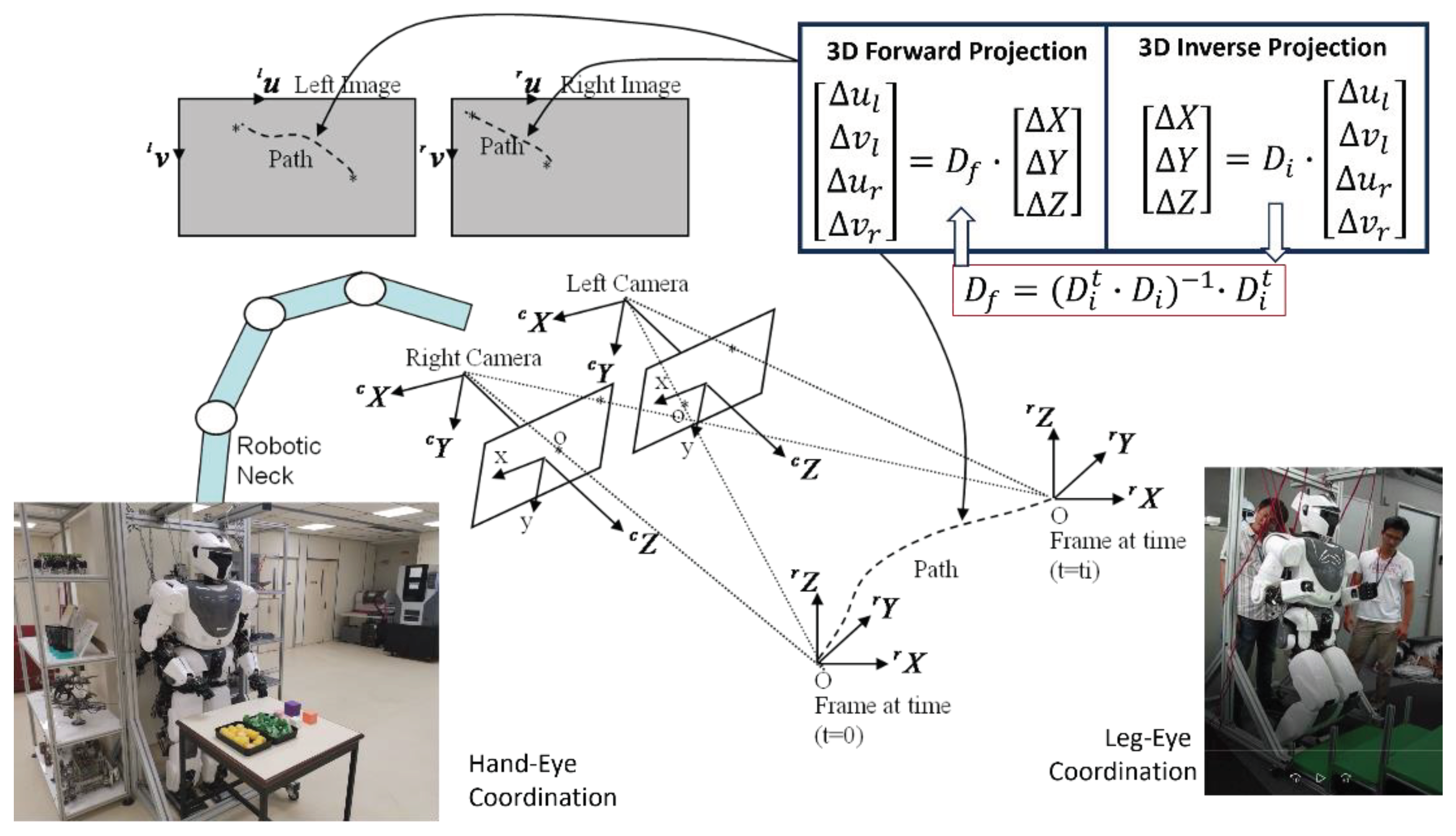
5. Experimental Results

The main purpose of this paper is to disclose the newly discovered solution to 3D projection in a human-like binocular vision. However, for the sake of making this paper more convincing, we present a set of preliminary experimental results in this section.

It is worth noting that this paper is not discussing about camera calibration which is a separate research topic having been widely investigated in the past decades [23,24,25,26,27]. Most importantly, the well-known procedures [24] of doing camera calibration have been implemented inside relevant toolbox of MATLAB [28].

It is also worth noting that camera calibration and vision system calibration are two different topics. Mathematically, vision system calibration implicitly includes the necessary details or benefits (e.g., non-linearity rectifications or optical distortion compensations) of camera calibration. However, from the viewpoint of vision-based applications, vision system calibration is more important than camera calibration. To the best of our knowledge, the newly discovered solution presented in this paper has not yet been known in the existing literature [29,30].

5.1. Real Experiment Validating Equation of 3D Inverse Projection of Position

Here, we would like to share an experiment in which we makes use of low-cost hardware with low-resolution binocular cameras and a small-sized checkerboard. In this way, we could appreciate the validity of Equation (20) and the theoretical result which is summarized in Figure 6.

As shown in Figure 8, the experimental hardware includes a Raspberry Pi single board computer, a binocular vision module, and a checkerboard. The image resolution of the binocular cameras is $480\times 320$ pixels. The checkerboard has the size of $18\times 24$ cm, which is divided into $6\times 8$ squares with the size of $3.0\times 3.0$ cm each.

Figure 8. Experimental hardware includes Raspberry Pi single board computer with a binocular vision module and a checkerboard which serves as input of calibration data-points as well as test data-points.

Figure 8. Experimental hardware includes Raspberry Pi single board computer with a binocular vision module and a checkerboard which serves as input of calibration data-points as well as test data-points.

Inside the checkerboard, $\{A,B,C,D\}$ serve as calibration data-points for the purpose of determining matrix $B_i$ in Equation (20), while $\{T_0,T_1,T_2,T_3,T_4\}$ serve as test data-points of the calibration result (i.e., to test the validity of matrix $B_i$ in Equation (20)).

Refer to Equation (20), matrix $B_i$ is a $4\times 5$ matrix in which there are nineteen independent elements or parameters. Since a single Equation (20) will impose three constraints, at least seven pairs of $\{X,Y,Z\}$ and $\{u_l,v_l,u_r,v_r\}$ are needed for us to fully determine matrix $B_i$.

As shown in Figure 9, we define a reference coordinate system as follows: Its Z axis is parallel to the ground and is pointing toward the scene. Its Y axis is perpendicular to the ground and is pointing downward. Its X axis is pointing toward the right-hand side.

Then, we place the checkerboard at four locations in front of the binocular vision system. The Z coordinates of these four locations are 1.0 m, 1.5 m, 2.0 m, and 2.5 m, respectively. The checkerboard is perpendicular to Z axis, which passes through test data-point $T_0$. Therefore, the X and Y coordinates of the calibration data-points $\{A,B,C,D\}$ and the test data-points $\{T_0,T_1,T_2,T_3,T_4\}$ are known in advance. The values of these X and Y coordinates are shown inside Figure 9.

Figure 9. Data set for calibrating matrix $B_i$ in Equation (20).

Figure 9. Data set for calibrating matrix $B_i$ in Equation (20).

When the checkerboard is placed at one of the above-mentioned four locations, a pair of stereo images is taken. The index coordinates of the calibration data-points and the test data-points could be determined either automatically or manually.

By putting the 3D coordinates and index coordinates of the calibration data-points together, we obtain Table 1 which contains the data needed for calibrating the equation of 3D inverse projection of binocular vision (i.e., Equation (20)).

With the use of data listed in Table 1, we obtain the following result of matrix $B_i$:

$$B_i=\left[\begin{array}{ccc}-0.4251& -0.7861& \begin{array}{ccc}-0.2245& 0.8267& 92.6220\end{array}\\ 0.2167& -0.3717& \begin{array}{ccc}-0.2730& 0.9845& -196.0451\end{array}\\ \begin{array}{c}-1.5409\\ -0.0874\end{array}& \begin{array}{c}14.4961\\ 0.1758\end{array}& \begin{array}{ccc}\begin{array}{c}1.2774\\ 0.0873\end{array}& \begin{array}{c}-14.9300\\ -0.1758\end{array}& \begin{array}{c}-71.2214\\ 1.0000\end{array}\end{array}\end{array}\right]$$

(24)

Now, we use the index coordinates in Table 1, calibrated matrix $B_i$, and Equation (20) to calculate the 3D coordinates of calibration data-points $\{A,B,C,D\}$. By combining these calculated 3D coordinates with data in Table 1, we will obtain Table 2 which helps us to compare between the true values of $\left\{A,B,C,D\right\}$’s 3D coordinates and the calculated values of $\{A,B,C,D\}$’s 3D coordinates.

In Table 2, the values in columns 2, 5 and 8 are the ground truth data of (X, Y, Z) coordinates of $\left\{A,B,C,D\right\}$. The values in columns 3, 6, and 9 are the computed values of $\left\{A,B,C,D\right\}$‘s (X, Y, Z) coordinates by using Equation (20).

Similarly, we use the index coordinates of the test data-points $\{T_0,T_1,T_2,T_3,T_4\}$, calibrated matrix $B_i$, and Equation (20) to calculate the 3D coordinates of $\{T_0,T_1,T_2,T_3,T_4\}$. Then, by combining the true values of $\{T_0,T_1,T_2,T_3,T_4\}$’s 3D coordinates and the calculated values of $\{T_0,T_1,T_2,T_3,T_4\}$’s 3D coordinates together, we obtain Table 3 which helps us to appreciate the usefulness and validity of Equation (20).

In Table 3, the values in columns 2, 5 and 8 are the ground truth data of (X, Y, Z) coordinates of ${\{T}_0,T_1,T_2,T_3,T_4\}$. The values in columns 3, 6, and 9 are the computed values of ${\{T}_0,T_1,T_2,T_3,T_4\}$‘s (X, Y, Z) coordinates by using Equation (20).

In view of the low-resolution of digital images (i.e., $480\times 320$ pixels) and a small-sized checkerboard (i.e., $18\times 24$ cm divided into $6\times 8$ squares), we could say that the comparison results shown in Table 2 and Table 3 are reasonably good enough for us to experimentally validate Equation (20). In practice, images with much higher resolutions and checkerboards of larger sizes will naturally increase the accuracy of binocular vision calibration as well as the accuracy of calculated 3D coordinates by using Equation (20).

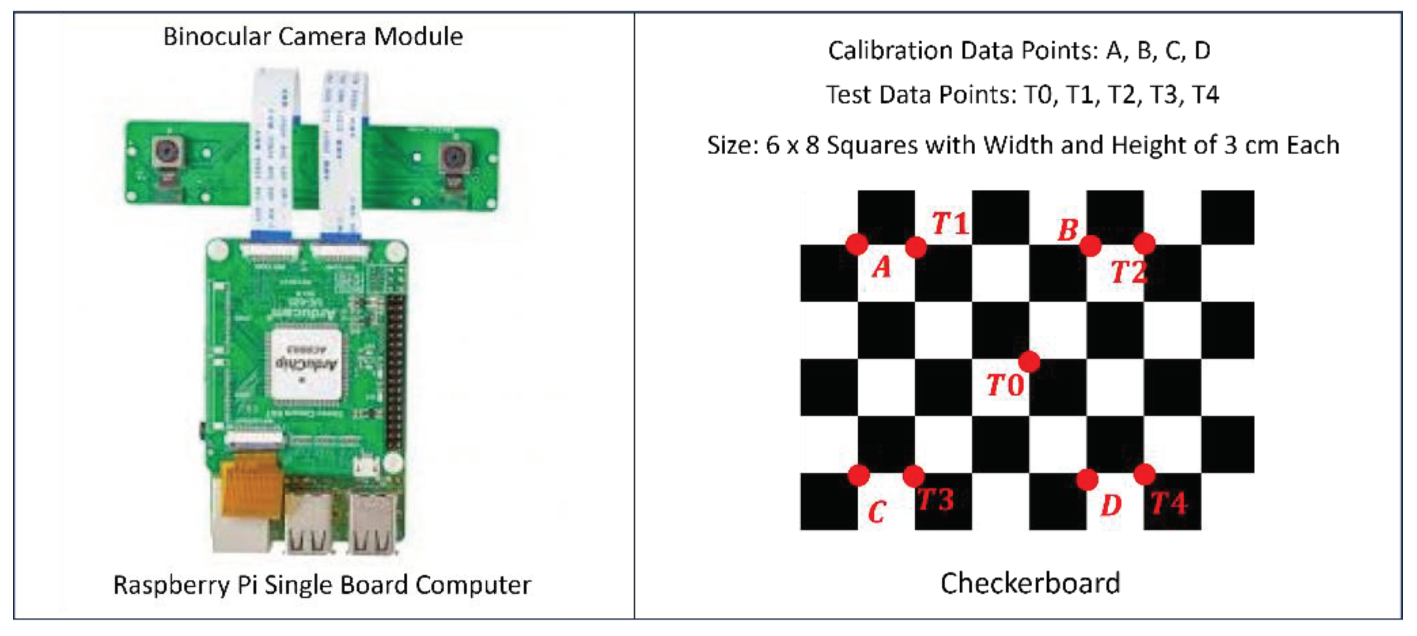
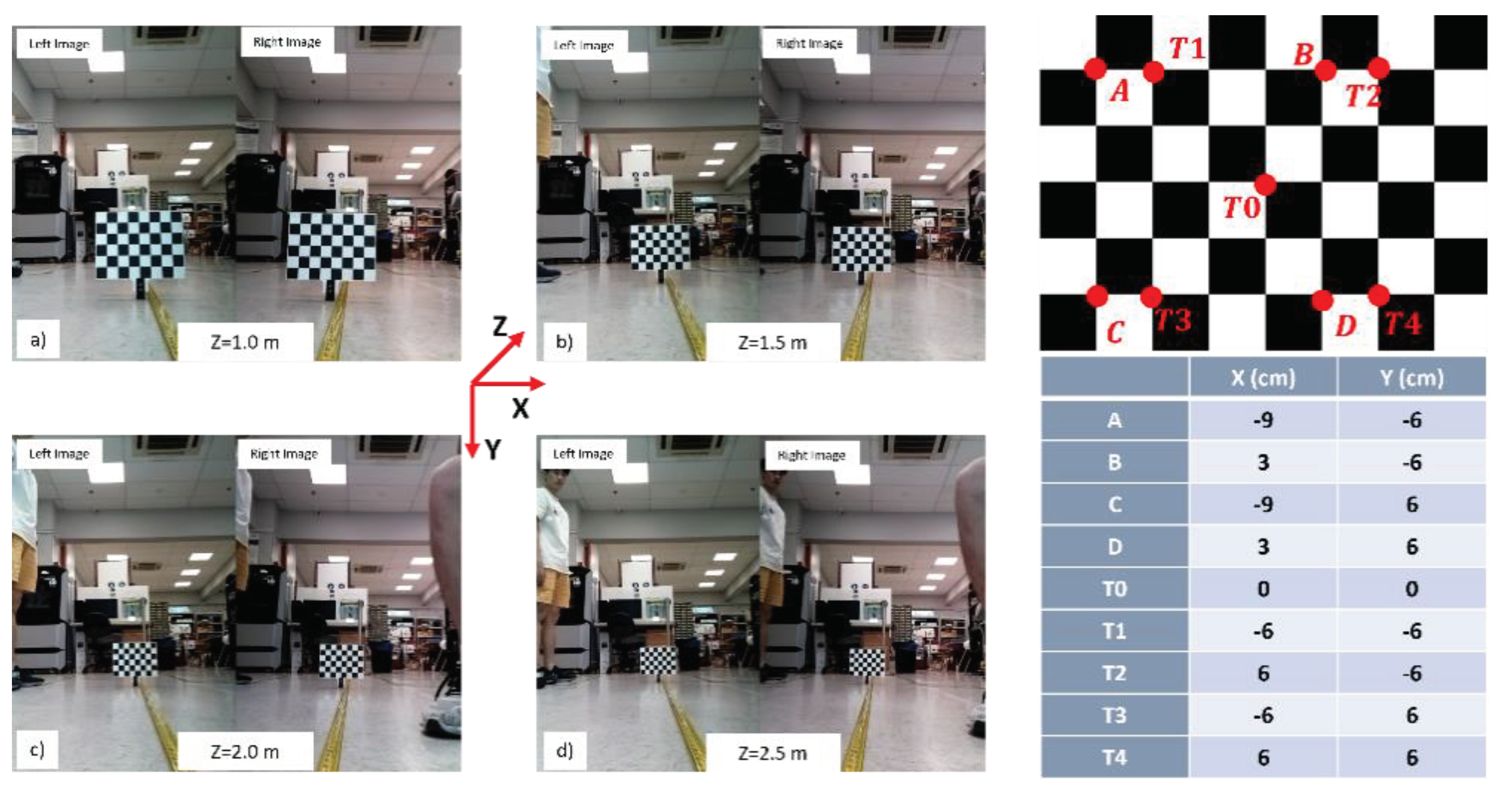
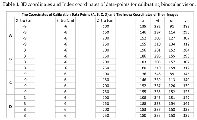
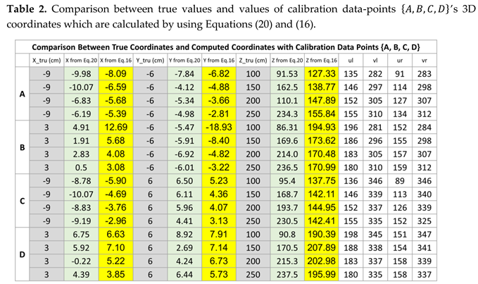
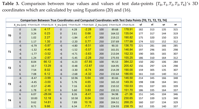
5.2. Comparative Study with Textbook Solution of Computing 3D Coordinates

For the sake of convincing the readers about the accuracy of 3D coordinates computed from using newly discovered Equation (20), we include the 3D coordinates computed from using Equation (16) which is the conventional method taught in textbooks of computer vision or robot vision.

The use of Equation (16) requires us to first calibrate the forward projection matrices of both left and right cameras. These two forward projection matrices are described in Equations (11) and (12). With the same dataset in Table 1, we obtain the following two forward projection matrices for both left and right cameras:

$$C_f^l=\left[\begin{array}{c}\begin{array}{cc}\begin{array}{cc}1.8405& 1.5144\end{array}& \begin{array}{cc}-1.3897& 168.4963\end{array}\end{array}\\ \begin{array}{cc}\begin{array}{cc}5.6358& 1.7619\end{array}& \begin{array}{cc}-2.6519& 323.8144\end{array}\end{array}\\ \begin{array}{cc}\begin{array}{cc}0.0177& 0.0091\end{array}& \begin{array}{cc}-0.0082& 1.0000\end{array}\end{array}\end{array}\right]$$

(25)

and

$$C_f^r=\left[\begin{array}{c}\begin{array}{cc}\begin{array}{cc}4.5384& 0.2891\end{array}& \begin{array}{cc}-0.8576& 145.8133\end{array}\end{array}\\ \begin{array}{cc}\begin{array}{cc}10.0682& 1.3962\end{array}& \begin{array}{cc}-1.8761& 318.5775\end{array}\end{array}\\ \begin{array}{cc}\begin{array}{cc}0.0321& 0.0038\end{array}& \begin{array}{cc}-0.0059& 1.0000\end{array}\end{array}\end{array}\right]$$

(26)

From the index coordinates listed in Table 1 and the two forward projection matrices in Equations (25) and (26), the use of Equation (16) will yield the computed 3D coordinates of calibration data-points $\{A,B,C,D\}$. By combining these calculated 3D coordinates with data in Table 1, we will obtain additional entries to Table 2 which help us to compare between the true values of $\left\{A,B,C,D\right\}$’s 3D coordinates and the calculated values of $\{A,B,C,D\}$’s 3D coordinates.

In Table 2, the values in columns 2, 5 and 8 are the ground truth data of (X, Y, Z) coordinates of $\left\{A,B,C,D\right\}$. The values in columns 4, 7, and 10 are the computed values of $\left\{A,B,C,D\right\}$‘s (X, Y, Z) coordinates by using Equation (16).

Similarly, from the index coordinates listed in Table 1 and the two forward projection matrices in Equations (25) and (26), the use of Equation 16 will yield the 3D coordinates of $\{T_0,T_1,T_2,T_3,T_4\}$. Then, by combining the true values of $\{T_0,T_1,T_2,T_3,T_4\}$’s 3D coordinates and the calculated values of $\{T_0,T_1,T_2,T_3,T_4\}$’s 3D coordinates together, we obtain additional entries to Table 3.

In Table 3, the values in columns 2, 5 and 8 are the ground truth data of (X, Y, Z) coordinates of ${\{T}_0,T_1,T_2,T_3,T_4\}$. The values in columns 4, 7, and 10 are the computed values of ${\{T}_0,T_1,T_2,T_3,T_4\}$‘s (X, Y, Z) coordinates by using Equation (16).

If we compare the data among columns 3, 4, 6, 7, 9 and 10 in Table 2, it is clear to us that the accuracy obtained from the newly discovered solution (ie., Equation (20)) in this paper is much better than the accuracy obtained from the conventional solution (i.e., Equation (16)). Especially, the errors in Z coordinates are largely reduced with the use of the proposed new solution.

Similarly, if we compute the data among columns 3, 4, 6, 7, 9 and 10 in Table 3, the same conclusion could be made, which is to say that the proposed solution will produce 3D coordinates of higher accuracy than the conventional solution in textbooks of computer vision or robot vision.

On top of the performance of achieving better accuracy than the textbook solution, the newly discovered solution simply requires one multiplication between a matrix and a vector. This is shown in Equation (20).

However, if we examine Equation (16), it is clear to us that the conventional way of computing the 3D coordinates at each point or pixel requires one transpose of matrix, one inverse of matrix, and three times of matrix multiplication. Hence, the newly discovered solution minimizes the computational workload for each set of 3D coordinates. This helps us to understand why human eyes do not experience fatigue or heating despite the huge quantity of visual signals coming from each eye’s imaging cells.

6. Conclusion

In this paper, we have proven two equations underlying 3D projections in binocular vision, which are Equations (20) and (22). Also, we have done experimental validation of the newly discovered solution which is to achieve 3D projections in binocular vision. Real experimental results reveal that the proposed solution produces 3D coordinates with better accuracy than the results which are computed with the use of textbook solution in computer vision or robot vision.

Most importantly, these two equations fully describe the 3D projections in a human-like binocular vision system. It is interesting to take note that Equations (20) and (22) are like the equations underlying 2D forward and inverse projections in a monocular vision system. These findings help us to unify the geometrical aspects of monocular vision and binocular vision in terms of equations for forward and inverse projections.

In addition, Equations (20) and (22) are in the form of two systems of linear equations, which could be easily implemented by a network of artificial neurons. As a result, the matrices in Equations (20) and (22) could be easily obtained by a calibration or learning process without the need of knowing the intrinsic parameters of the cameras inside binocular vision systems.

In humanoid robotics, a binocular vision system is mounted inside the head of a humanoid robot. Hence, the fingertips of the humanoid robot will be able to readily provide the necessary datasets for the calibration or learning of both Equations (20) and (22). This implies that periodic calibration or learning on the fly or on the go is not a difficult issue under the context of humanoid robotics.

Obviously, the theoretical findings in this paper will motivate us to further investigate the truth behind the phenomenon which is to say that a huge quantity of visual signals from human vision will not cause fatigue to human beings’ brains. These findings could further motivate us to investigate the answer to the question of why human vision could adapt to the growth of human being’s body.

Although the works presented in this paper are inspired by human vision, we hope that more and more research works will be dedicated to the discovery of the secrets behind human beings’ visual systems in terms of real-time responses and low-power consumption. Last but not the least, we believe that Equations (20) and (22) will contribute to future research and product development of binocular vision systems dedicated to humanoid robots and other types of robots.

References

- Xie, M. Hu, Z. C. and Chen, H. New Foundation of Artificial Intelligence. World Scientific, 2021.
- Horn, B. K. P. Robot Vision. The MIT Press, 1986.
- Tolhurst, D. J. Sustained and transient channels in human vision. Vision Research, 1975; Volume 15, Issue 10, pp1151-1155.
- Fahle M and Poggio, T. Visual hyperacuity: spatiotemporal interpolation in human vision, Proceedings of Royal Society, London, 1981.
- Enns, J. T. and Lleras, A. What’s next? New evidence for prediction in human vision. Trends in Cognitive Science 2008, 12, 327–333. [Google Scholar] [CrossRef] [PubMed]
- Laha, B. , Stafford, B. K. and Huberman, A. D. Regenerating optic pathways from the eye to the brain. Science, 2017, 356, 1031–1034. [Google Scholar] [CrossRef] [PubMed]
- Gregory, R. Eye and Brain: The Psychology of Seeing - Fifth Edition, The Princeton University Press, 2015.
- Pugh, A. (editor). Robot Vision. Springer-Verlag, 2013.
- Samani, H. (editor). Cognitive Robotics. CRC Press, 2015.
- Erlhagen, W. and Bicho, E. The dynamic neural field approach to cognitive robotics. Journal of Neural Engineering 2006, 3.
- Cangelosi, A. and Asada, M. Cognitive Robotics. The MIT Press, 2022.
- Faugeras, O. Three-dimensional Computer Vision: A Geometric Viewpoint. The MIT Press, 1993.
- Paragios, N. , Chen, Y. M. and Faugeras, O. (editors). Handbook of Mathematical Models in Computer Vision. Springer, 2006.
- Faugeras, O. Luong, Q. T. and Maybank, S. J. Camera self-calibration: Theory and experiments. European Conference on Computer Vision. Springer, 1992; LNCS, Volume 588.
- Stockman, G. and Shapiro, L. G. Computer Vision. Prentice Hall, 2001.
- Shirai, Y. Three-Dimensional Computer Vision. Springer, 2012.
- Khan, S. Rahmani, H., Shah, S. A. A. and Bennamoun, M. A Guide to Convolutional Neural Networks for Computer Vision. Springer, 2018.
- Szeliski, R. Computer Vision: Algorithms and Applications. Springer, 2022.
- Brooks, R. New Approaches to Robotics. Science 1991, 253. [Google Scholar] [CrossRef] [PubMed]
- Xie, M. Fundamentals of Robotics: Linking Perception to Action. World Scientific, 2003.
- Siciliano, B. and Khatib, O. Springer Handbook of Robotics. Springer, 2016.
- Murphy, R. Introduction to AI Robotics - Second Edition. The MIT Press, 2019.
- Clarke, T. A. and Fryer, J. G. (1998). The development of camera calibration methods and models. The Photogrammetric Record, Wiley Online Library.
- Zhang, Z. Y. , A flexible new technique for camera calibration. IEEE Transactions on Pattern Recognition and Machine Intelligence 2000, 22, 1330–1334. [Google Scholar] [CrossRef]
- Wang, Q,, Fu, L. and Liu Z. Z (2010). Review on camera calibration, 2010 Chinese Control and Decision Conference, Xuzhou, 2010, pp. 3354-3358. [CrossRef]
- Cui, Y., Zhou, F. Q., Wang, Y. X., Liu, L., and Gao, H. Precise calibration of binocular vision system used for vision measurement, Optics Express 2014, 22, 9134-9149.
- Zhang, Y. J. (2023). Camera Calibration. In: 3-D Computer Vision. Springer, Singapore.
- Fetić, A. Jurić, D. and Osmanković, D. (2012). The procedure of a camera calibration using Camera Calibration Toolbox for MATLAB, 2012 Proceedings of the 35th International Convention MIPRO, Opatija, Croatia, pp. 1752-1757.
- Xu, G., Chen. J. and Li, X. 3-D Reconstruction of Binocular Vision Using Distance Objective Generated From Two Pairs of Skew Projection Lines, IEEE Access 2017, 5, 27272–27280. [Google Scholar] [CrossRef]
- Xu, B. Q. and Liu, C. A 3D reconstruction method for buildings based on monocular vision. Computer-aided Civil and Infrastructure Engineering 2021, 37, 354–369. [Google Scholar] [CrossRef]
Disclaimer/Publisher’s Note: The statements, opinions and data contained in all publications are solely those of the individual author(s) and contributor(s) and not of MDPI and/or the editor(s). MDPI and/or the editor(s) disclaim responsibility for any injury to people or property resulting from any ideas, methods, instructions or products referred to in the content. |
© 2024 by the authors. Licensee MDPI, Basel, Switzerland. This article is an open access article distributed under the terms and conditions of the Creative Commons Attribution (CC BY) license (http://creativecommons.org/licenses/by/4.0/).