1. Introduction
Complex networks can effectively represent many real-world networks, such as the Internet, social networks, power grids, and so on. Most networks are beneficial to people and bring many positive effects. However, some networks also have negative effects, with the most important examples being terrorism and disease transmission networks [
1,
2]. Whether beneficial or harmful, these networks substantially influence the functioning and development of our society. In recent decades, the study of diverse complex networks has gained significant attention from researchers across various fields such as computer science, statistical physics, systems engineering, and applied mathematics [
3,
4,
5,
6,
7]. One hot topic point in these studies is the error and attack tolerance of complex networks [
8,
9,
10,
11,
12,
13,
14,
15,
16], a concept referred to as
robustness within the context of this paper.
The robustness of a network refers to its ability to keep functioning when some of its components, such as nodes or edges, malfunction due to random failures or malicious attacks [
12,
17,
18]. The study of network robustness is valuable from two main perspectives. Firstly, the failure of components can lead to the breakdown of beneficial networks and result in significant economic losses. A typical example is the Northeast blackout of 2003 [
19,
20]. Analyzing network robustness aids in developing methods to enhance it. On the other hand, for harmful networks, such as terrorist networks [
21] or COVID-19 transmission networks [
22], analyzing their robustness assists in developing effective attack strategies to dismantle them. Therefore, analyzing network robustness is of great importance.
To analyze the robustness of the network, it is necessary to choose a suitable metric to evaluate how robust a network is. Since almost all network applications are typically designed to operate in a connected environment [
23], network connectivity is selected as the primary indicator to assess network robustness in this study.
The robustness of a network depends not only on its structural features but also on the mechanisms of random failures or malicious attacks. In random failures, nodes or edges are attacked with equal probability, while malicious attacks target nodes or edges in decreasing order of their importance. Typically random failures are less severe than malicious attacks [
24,
25]. Evaluating the impacts of node or edge removal using various malicious attack strategies is a crucial approach to analyzing network robustness. Determining the lower bound of network robustness is critical as it allows for analysis of network robustness under worst-case scenarios, identification of the most vulnerable components, and development of robustness improvement methods. An effective approach to addressing this issue involves identifying an optimal attack strategy that inflicts maximum damage on the network [
26].
Extensive research has been conducted on the robustness of complex networks. Albert et al. [
8] studied the robustness of scale-free networks and found that while these networks are robust to random failures, they are extremely vulnerable to malicious attacks. Iyer et al. [
9] conducted a systematic examination of the robustness of complex networks by employing simultaneous and sequential targeted attacks based on various centrality measures such as degree, betweenness, closeness, and eigenvector centrality. Fan et al. [
10] proposed a deep reinforcement learning algorithm, FINDER, to effectively identify critical network nodes. Wang et al. [
11] introduced region centrality and proposed an efficient network disintegration strategy based on this concept, which combines topological properties and geographic structure in complex networks. Ma et al. [
12] conducted a study on the robustness of complex networks against incomplete information. They employed link prediction methods to restore missing network topology information and identify critical nodes. Lou et al. [
14] introduced LFR-CNN, a CNN-based approach that utilizes learning feature representation for predicting network robustness, which exhibits excellent predictive performance notably smaller prediction errors.
However, the aforementioned research generally assumes that attacks on the network will always be successful, neglecting the important factor of attack success rate (ASR). In fact, an attack may not succeed in real-world scenarios. For example, even if the enemy forces launch an attack on a target within a military communication network, there is no guarantee of successfully destroying it.
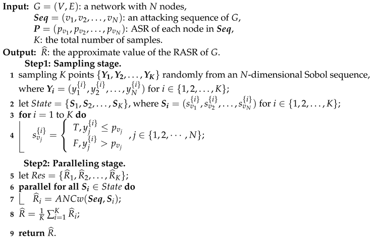
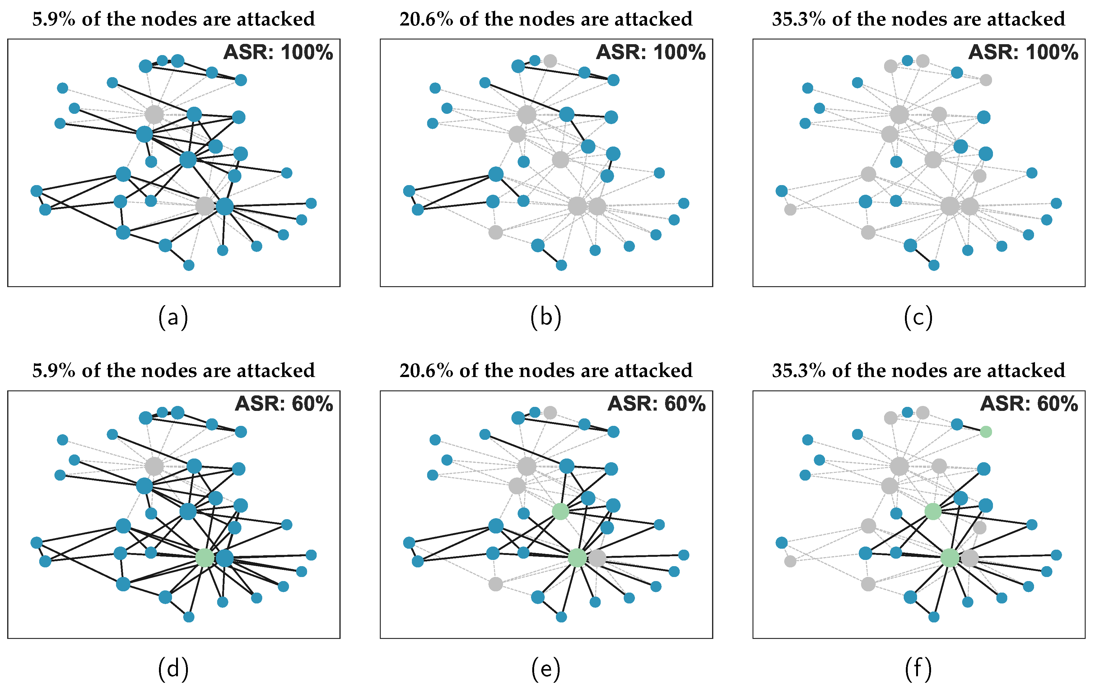
Figure 1 illustrates the main process of network disintegration under varying ASR. Moreover, selecting an optimum attack strategy that can lead to maximal destructiveness to the network is challenging due to the NP-hard nature of this problem [
10]. Existing methods often encounter difficulties in achieving a desirable balance between effectiveness and computational efficiency.
Therefore, the purpose of this paper is to analyze network robustness when considering ASR under an optimal attack strategy. To achieve this purpose, a novel robustness measure called Robustness-ASR (RASR) is introduced, which utilizes mathematical expectations to evaluate network robustness when considering ASR. In addition, an efficient algorithm called PRQMC is proposed to calculate the RASR for large-scale networks. Furthermore, to assess the lower bound of network RASR, a new attack strategy, named HBnnsAGP, is proposed. The main contributions of this study are as follows:
We introduce and define a novel robustness measure called RASR, which utilizes mathematical expectations to assess network robustness when considering the ASR of each node.
To efficiently calculate the RASR for large-scale networks, we propose the PRQMC algorithm. PRQMC leverages randomized quasi-Monte Carlo (QMC) integration to approximate the RASR with a faster convergence rate and utilizes parallelization to speed up the calculation.
To assess the lower bound of network RASR, we present a new attack strategy, named HBnnsAGP. In HBnnsAGP, a novel centrality measure called BCnns is proposed to quantify the importance of a node.
The experimental results on 6 representative real-world networks demonstrate the effectiveness of the proposed methods compared with the baselines.
The rest of this paper is organized as follows.
Section 2 provides an introduction to the preliminaries, including classical centrality measures, traditional network robustness measures, and the principles of Monte Carlo (MC) and QMC integration.
Section 3 presents the proposed methods for analyzing network robustness when considering ASR, including the RASR, the PRQMC algorithm, and the HBnnsAGP attack strategy. The experiments and results are demonstrated in
Section 4. Finally,
Section 5 concludes the paper.
2. Preliminaries
A complex network can be modeled as an unweighted undirected graph , where and represent the set of nodes and the set of edges in the network G, respectively. The network G can be also represented as an adjacency matrix , if node i and node j are connected, , otherwise .
2.1. Centrality Measures
The concept of a centrality measure attempts to quantify how important a node is [
27]. Here we introduce two classical centrality measures: degree centrality and betweenness centrality.
2.1.1. Degree centrality (DC)
DC is the simplest measure of centrality. The DC of a node is defined by its degree, that is, its number of edges. The DC is formally defined as follows.
Definition 1.
Given a network , is the adjacency matrix of the network G. The DC of node i is defined as:
The DC is frequently a reliable and effective measure of a node’s importance. A higher DC value typically signifies a more critical node.
2.1.2. Betweenness centrality (BC)
BC quantifies the number of shortest paths passing through a particular node in a network[
28]. BC characterizes the extent to which a node acts as a mediator among all other nodes in a network[
27]. Nodes that lie on numerous shortest paths are likely to play a crucial role in information transmission, exhibiting higher BC values. The BC is defined as follows.
Definition 2.
Given a network . The BC of node v in G is defined as:
where, , is the total number of shortest paths from node s to node t and is the number of those paths that pass through node v. , if . , if .
2.2. Accumulated Normalized Connectivity
Traditionally, network robustness has been evaluated by calculating the size of the giant connected component (GCC) after the network has endured attacks. The Accumulated Normalized Connectivity (ANC), also known as
R, is a well-known measure of network robustness for node attacks [
10,
17,
29]. The ANC is defined as follows.
Definition 3.
For a network , . Given an attack sequence of nodes , where indicates the ith node to be attacked, the ANC of G under this attack sequence is defined as:
here, is the size of the GCC of the residual network after the sequential removal of nodes from the set in G, and the initial size of the GCC of G before any nodes are removed. The normalization factor ensures that the robustness of networks with different sizes can be compared.
A larger ANC value indicates a higher level of network robustness against attacks. Additionally, the ANC can be used to assess the destructiveness of attacks, lower ANC values correspond to more destructive attack strategies. The ANC value can be viewed as an estimate of the area beneath the ANC curve, which is plotted with the horizontal axis as and the vertical axis as .
2.3. Monte Carlo Integration
Monte Carlo (MC) integration is a numerical technique that is particularly useful for higher-dimensional integrals[
30]. Caflisch[
31] provides a comprehensive review of this method. The integral of a Lebesgue integrable function
can be expressed as the average or expectation of the function evaluated at random locations. Considering
as a random variable uniformly distributed on the one-dimensional unit interval
, the integration of
over this interval can be represented as follows:
in which
is the probability measure of
on the interval
, then
therefore
Similarly, for an integral on the unit hypercube
in
N dimensions,
in which
is a uniformly distributed vector in
, where
. Given that the hyper-volume of
is equal to 1, thus
can be viewed as the total probability space.
The MC integration method approximates definite integrals utilizing random sampling. It draws
K uniform samples from
, in turn generating a points set
. The empirical approximation of the integral
is then procured by computing the mean of the
K sample outcomes
, which can be expressed as follows:
According to the Strong Law of Large Numbers [
32], this approximation is convergent with probability 1, that is,
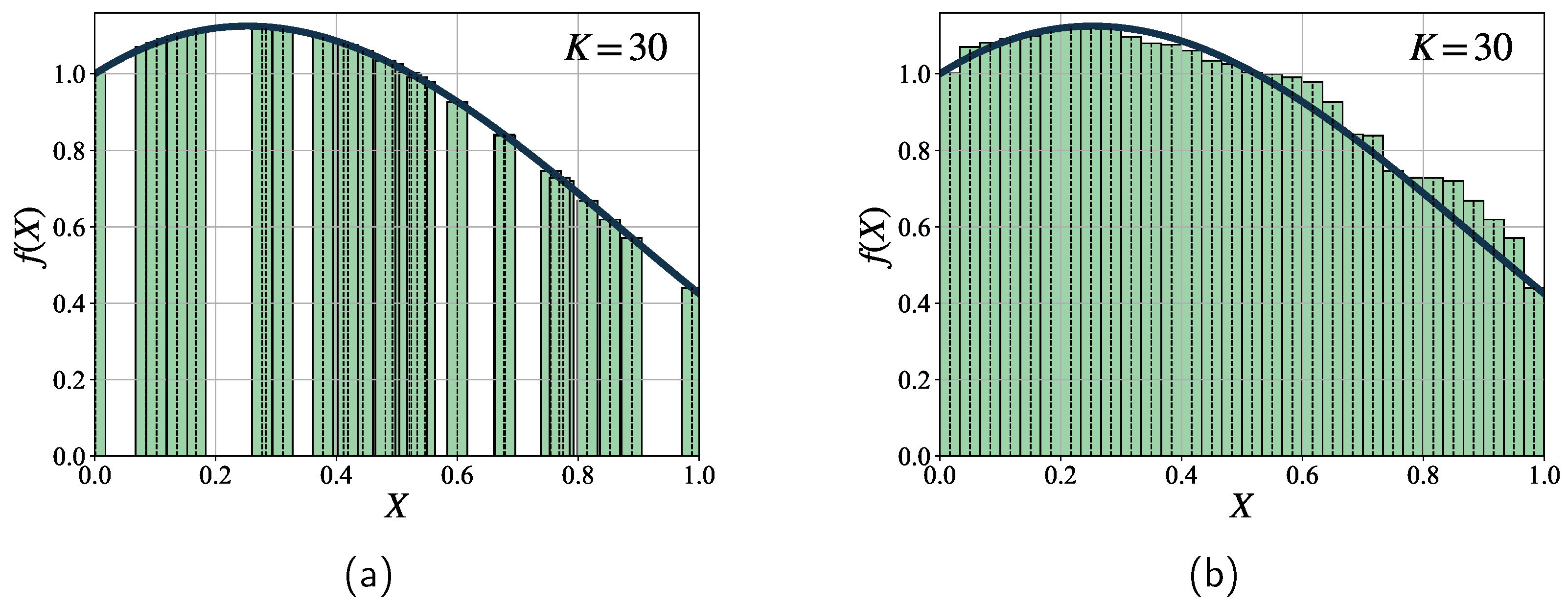
Figure 2 illustrates the application of the MC integration method in approximating definite integrals over a one-dimensional unit interval. As shown in
Figure 2a, MC integration approximates the area under the curve of the integral by summing the areas of the bars corresponding to the sampled points. The bars are rearranged sequentially to avoid overlap on the
-axis, as shown in
Figure 2b.
The error of MC integration is
By the Central Limit Theorem [
32], for any
where
, we have
where
v is a standard normal random variable and
is the square root of the variance of
f, given by
When
K is sufficiently large, we have
This implies that the order of error convergence rate of the MC integration is
[
33], which means that the accuracy of the integral error decreases at a rate proportional to the total number of samples
K increases. That is, “an additional factor of 4 increase in computational effort only provides an additional factor of 2 improvements in accuracy" [
31].
In practical applications, the MC integration method draws K uniform samples from an N-dimensional pseudo-random sequence (PRS) generated by a computer to obtain the points set .
2.4. Quasi-Monte Carlo Integration
The quasi-Monte Carlo (QMC) integration is a method of numerical integration that operates in the same way as MC integration, but instead uses a deterministic low-discrepancy sequence (LDS) [
34] to approximate the integral. The advantage of using LDSs is a faster rate of convergence. QMC integration has a rate of convergence close to
, which is much faster than the rate for the MC integration,
[
35]
Using the QMC integration method for approximating definite integrals is similar to the MC integration method. This can be expressed as:
where
is a points set obtained by combining the first
K points from an
N-dimensional LDS. Each
is an
N-dimensional point, with
for
, and
for
.
The error order of the QMC integration can be determined by the Koksma-Hlawka inequality [
36,
37], that is,
where
is the Hardy–Krause variation of the function
f,
is the star discrepancy of
, and is defined as:
where
is the number of points in
inside the region
Q, and
is the Lebesgue measure of region
Q in the unit hypercube
. For more detailed information, please refer to [
31].
For an
N-dimensional LDS comprising
K points, the star discrepancy of the sequence is
. Consequently, for a function
F with
, a QMC approximation based on this sequence yields a worst-case error bound in Equation (
28) converging at a rate of
[
38]. Since
, the QMC integration convergence rate approaches
for low-dimensional cases [
33], which is asymptotically superior to MC.
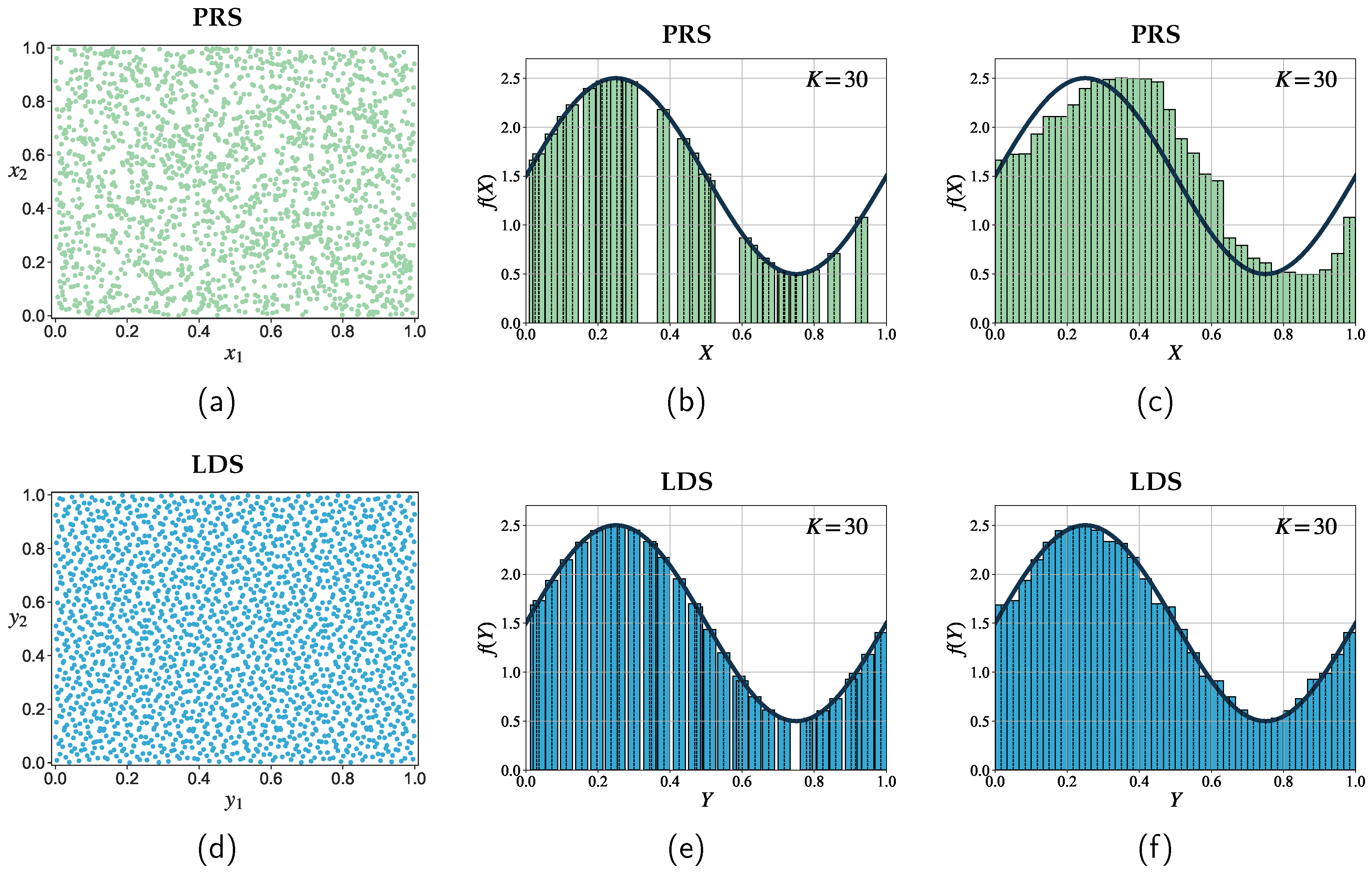
Figure 3 illustrates the clear differences between MC and QMC integration methods. The subfigures provide a visual representation of their respective point distributions and demonstrate their application for approximating definite integrals over a one-dimensional unit interval. The points generated from an LDS exhibit greater uniformity than the points generated by a PRS. Consequently, with the same number of sampling points, LDS has the ability to uniformly fill the integration space, resulting in a faster convergence rate.
3. Methods
In this section, we will first introduce the major problem we focus on in this paper. Then, we give the details of the proposed methods for analyzing network robustness when considering ASR, including the RASR, the PRQMC algorithm, and the HBnnsAGP attack strategy.
3.1. Problem Formalization
Typically, it is assumed that removing a node will also remove all of its connected edges. Therefore, in this paper, we only consider node attack strategies.
For a network
,
. A node attack strategy can be represented as a sequence
, where
indicates the
ith node to be attacked. Given a predefined metric
to measure network robustness against attacks. The primary goal is to evaluate the lower bound of network robustness. Therefore, the objective is to minimize
, as presented below:
To achieve this objective, it is crucial to determine the optimal node attack strategy that will minimize the
.
3.2. The Proposed Robustness Measure RASR
The ANC, as defined in Definition 3, does not consider the ASR, or it is a special case where the ASR of each node is 100%. To this end, the proposed robustness measure RASR utilizes mathematical expectations to assess network robustness when considering ASR. Before introducing the RASR, we will first present a weighted ANC (named ANCw), which takes into account both the state of the attack sequence state and the associated attack cost.
For a network
with
N nodes,
is an attack sequence, where
. The state of
is denoted as a random variable
, where
Then, the ANCw is defined as follows.
Definition 4.
The ANCw of G under an attack sequence is defined as:
here is the same as defined in Definition 3. When k = 0, it indicates that no nodes have been attacked. is a weighted function, that is,
There are two main reasons for using the weighted function
. Firstly, it is important for an attacker to choose an optimal attack strategy at a minimum attack cost to efficiently disintegrate the network [
11,
26]. Secondly, as illustrated in
Figure 1, with an increased number of nodes removed, the network will eventually fragment into isolated nodes, thereby losing its functionality as a network. Therefore, this paper sets the attack cost of an isolated node to 0.
Let
represent the ASR of each node corresponding to
, where
represents the ASR of node
. Assuming that attacks on different nodes are independent, then the probability of
is
where
Based on the above formulas, the proposed RASR can defined as follows.
Definition 5.
Considering the ASR of each node, the robustness of a network G against an attack sequence can be quantified by the RASR, which is defined as:
where is a random variable representing the state of , Ω is the sample space of , is the expectation of the ANCw.
In theory, the value of RASR can be calculated using Equation (
23) once all the samples of
are obtained in the sample space
. However, it confronts “the curse of dimensionality" [
39] when applied to networks with a large number of nodes. In such cases, the size of
grows exponentially to
. As a result, the analytical approach becomes infeasible when
N is significantly large.
3.3. The Proposed PRQMC Algorithm
To efficiently calculate the RASR for large-scale networks, the PRQMC algorithm is proposed, which leverages randomized QMC integration to approximate the RASR with a faster convergence rate and utilizes parallelization techniques to speed up the calculation. In the following, we first introduce the RASR calculation model based on QMC integration and then give the PRQMC algorithm.
3.3.1. RASR Calculation Model Based on QMC Integration
The RASR of a network
G, as defined in Definition 5, can be expressed using Lebesgue integration based on the principle of MC integration (see
Section 2), that is,
where
denotes a random variable representing the state of an attacking sequence
,
is the sample space of
,
is the probability measure of
.
Let
represent the ASR of each node corresponding to
,
is a uniformly distributed vector in
, where
. Then,
can be represented as follows:
where
When the
is determined, the
can be represented as a function of
, that is,
By substituting Equation (
27) into Equation (
24) and transforming the integral space from
to
, we obtain the following expression for RASR:
This equation represents the integration of
with respect to the probability measure
over the
N-dimensional unit hypercube
.
For the given network
G, the sample space
has a size of
. Let the state of
be
, where
. Based on
, the unit hypercube
can be divided into
regions denoted by
, where region
corresponds to state
,
.
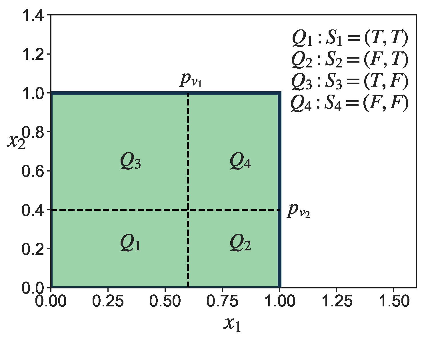
Figure 4 illustrates this process for the case when
. Then, the integral in Equation (
28) can be transformed into:
where
is a vector uniformly distributed within region
.
The Lebesgue measure of region
in
, denoted by
, is equivalent to the probability measure of
, denoted as
. Based on the principle of MC integration, we have:
Combining Equation (
28), Equation (
29), and Equation (
30), we obtain:
By referencing Equation (
14) and Equation (
31), the RASR of a network can be approximated using the QMC integration method. The approximation of RASR, denoted by
, is defined as follows.
Definition 6.
Consider a network with N nodes. Suppose a sequence of nodes is targeted for attack, signifies the ASR of each node. The RASR of the network G can be approximated by , which is defined as:
Here, , as specified in Equation (14), represents a set of points obtained from an N-dimensional LDS. K is the total number of samples. The function is defined in Equation (27).
The error bound of the QMC integral is determined by the star discrepancy of the chosen LDS, making the selection of LDSs important for improving the accuracy of approximations. Two frequently used LDSs are the Halton sequence and the Sobol sequence [
40]. In this research, the Sobol sequence is adopted, as it demonstrates better performance in higher dimensions compared to the Halton sequence [
41].
3.3.2. Parallel Randomized QMC (PRQMC) Algorithm
Despite the faster convergence rate of the QMC integration method compared to MC integration, it still necessitates a large number of samples to calculate the average value. Furthermore, the calculation of function
, typically done through attack simulations, demands considerable computational resources, especially for large-scale networks [
42]. Consequently, the computational process of obtaining
for large-scale networks remains time-consuming. Additionally, due to the deterministic nature of the LDS, the QMC integration method can be seen as a deterministic algorithm, thus presenting challenges in assessing the reliability of numerical integration results and potentially leading to being stuck in local optima. In light of these issues, the PRQMC algorithm capitalizes on the benefits of the Randomized QMC method and parallelization.
The PRQMC algorithm improves computational efficiency through parallelization. This is because the computational cost of sampling the attack sequence’s state is significantly lower than that of computing the function . Therefore, by initially sampling the attack sequence’s state and obtaining a sufficient number of samples, it is possible to calculate the by parallelizing the computation of the function with various samples. This approach effectively accelerates the calculation process by distributing the task across multiple processors or computing nodes.
Additionally, the PRQMC algorithm enhances randomness by randomly sampling points from the LDS, providing unbiased estimation and improved variance reduction capabilities. This is particularly advantageous in high-dimensional problems, where RQMC often outperforms QMC in terms of accuracy and efficiency [
43].
The procedure of the PRQMC algorithm is presented in Algorithm 1, which consists of two main steps: “sampling state" and “paralleling stage". In the sampling stage, we first randomly sample
K points
from an
N-dimensional Sobol sequence, then determine
K states of the attack sequence,
, by comparing the values of each dimension of the sampled points with the ASR of each node. In the paralleling stag, we parallelize the computation of the function
, then obtain
by calculating the average value of
.
|
Algorithm 1 PRQMC() |
 |
3.4. The Proposed HBnnsAGP Attack Strategy
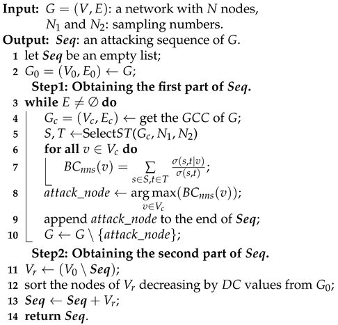
To assess the lower bound of network RASR, a new attack strategy called the High BCnns Adaptive GCC-Priority (HBnnsAGP) is presented. In HBnnsAGP, a novel centrality measure called BCnns is proposed to quantify the significance of a node, and GCC-priority attack strategy is utilized to improve attack effectiveness. Algorithm 2 describes the procedure of HBnnsAGP, which contains two steps: “obtaining the first part of
" and “obtaining the second part of
". In the first step, the algorithm obtains the first part of the attack sequence by iteratively removing the node with the highest BCnns in GCC and recalculating BCnns for the remaining nodes until only isolated nodes remain in the residual network. In the second step, the algorithm arranges these isolated nodes in descending order according to their DC values in the initial network to obtain the second part of the attack sequence. This procedure is aimed at improving the effectiveness of attacks when the ASR is below 100%. It is important to note that isolated nodes when the ASR is 100% may no longer remain isolated, as depicted in, as shown in
Figure 1. Additionally, previous research has shown that there is minimal difference in destructiveness between simultaneous attacks and sequential attacks based on DC [
9]. Therefore, by sorting these isolated nodes in descending order based on their DC values from the initial network (similar to the approach used in simultaneous attacks), the second step further improves the effectiveness of attacks when the ASR is less than 100%.
In the following, we first introduce the BCnns and then give the GCC-priority attack strategy.
|
Algorithm 2 HBnnsAGP() |
 |
3.4.1. Non-central Nodes Sampling Betweenness Centrality (BCnns)
Contrasted with BC (see Definition 2), which evaluates a node’s role as a mediator in the network based on the count of shortest paths it traverses for all node pairs. BCnns quantifies the importance of nodes acting as bridge nodes between different network communities by counting the number of shortest paths that pass through a node for specific pairs of non-central nodes (nodes located in the periphery of the network and with less importance). These bridge nodes typically serve as mediators for non-central nodes across different communities. The BCnns is defined as follows.
Definition 7.
For a network with N nodes, the BCnns of node v in network G is:
where , is the set of non-central nodes sampled from V, , . The and have the same meaning as defined in Definition 2.
By selecting the appropriate pairs of non-central nodes, BCnns can more effectively measure the significance of nodes as bridges between different communities in a network. While these bridge nodes may not have the highest BC value, they are crucial for maintaining overall network connectivity and could potentially have the highest BCnns value.
The Definition of BCnns highlights the importance of selecting suitable nodes for sets
S and
T. Thus, we proposed an algorithm called Selection
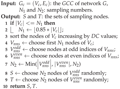
for node selection. Algorithm 3 describes the procedure of Selection
. Initially, the nodes are sorted in ascending order based on their DC values, and the first
nodes with lower DC values are selected to create the non-central nodes set
. This is because nodes with lower DC values typically have lower centrality and are considered non-central nodes. Next, in order to achieve a more balanced sampling,
is divided into two subsets:
containing nodes at odd indices and
containing nodes at even indices. Lastly,
nodes are randomly sampled from
to create set
S, and
nodes are similarly sampled from
to form set
T.
|
Algorithm 3 Selection() |
 |
The and are chosen based on the size of the network and the node degree distribution. Typically, both and are much smaller compared to the total number of nodes N. Therefore, BCnns have higher computational efficiency compared to BC, especially for large-scale networks.
Figure 5 demonstrates the differences between BC and BCnns. Specifically,
Figure 5a identifies the non-central nodes in red,
Figure 5b showcases node sizes based on BC values, and
Figure 5c adjusts node sizes based on their BCnns values. Notably, node 14 plays a critical bridging role between two communities, a role that BCnns captures more accurately than BC.
3.4.2. GCC-Priority Attack Strategy
As the attack progresses, the network fragments into connected components of varying sizes. The importance of these components varies within the residual network. The GCC refers to the largest connected component containing the most nodes. The destruction of the GCC accelerates the collapse of the network. The GCC-priority attack strategy enhances the attack’s effectiveness by targeting nodes within the GCC at each stage of the attack process.
4. Experimental Studies
In this section, we present a series of experiments to verify the effectiveness of our proposed methods. Firstly, we introduce the experimental settings including network datasets and baselines. Next, we compare the proposed PRQMC method with the baselines. Additionally, we demonstrate the effectiveness of the proposed HBnnsAGP attack strategy. Finally, we present further discussions on network robustness when considering the ASR.
4.1. Experimental Settings
4.1.1. Datasets
In our experiments, we selected six real-world classic complex networks of different scales, including Karate [
44], Krebs [
10], Airport [
45], Crime [
46], Power [
47], Oregon1 [
48].
Table 1 provides a detailed summary of these networks, with
N and
M representing the number of nodes and edges, respectively, and
denoting the average degree of the network.
4.1.2. Comparison Methods
To show the effectiveness of the proposed PRQMC algorithm, we compare it with MC and QMC methods.
MC: It calculates the estimated value of using original MC integration and generates a set of points from a PRS.
QMC: It calculates the estimated value of using original QMC integration and generates a set of points from an LDS.
To show the effectiveness of the proposed HBnnsAGP attack strategy, we compare it with three representative baseline attack strategies, including HDA[
49], HBA[
28], and FINDER[
10].
High Degree Adaptive (HDA): HDA is an adaptive version of the high degree method that ranks nodes based on their DC and sequentially removes the node with the highest DC. HDA recomputes the DC of the remaining nodes after each node removal and is recognized for its superior computational efficiency.
High Betweenness Adaptive (HBA): HBA is an adaptive version of the high betweenness method. It operates by iteratively removing the node with the highest BC and recomputing BC for the remaining nodes. HBA has long been considered the most effective strategy for the network dismantling problem in the node-unweighted scenario [
50]. However, the high computing cost prohibits its use in medium and large-scale networks.
FINDER: FINDER is notable as an algorithm based on deep reinforcement learning, which achieves superior performances in terms of both effectiveness and efficiency.
We implemented the proposed algorithm and baselines using the Python programming language. All experiments are performed on a server AMD EPYC 7742 64-Core Processor @ 2.25GHz, with memory (RAM) 1024 GB, running Linux ubuntu 11.10 Operating System.
4.2. Comparison of the PRQMC with Baselines
This subsection presents the comparison results to demonstrate the effectiveness of the proposed algorithm, PRQMC, on six real-world complex networks. Specifically, we compare PRQMC with two baselines: MC and QMC. All experiments use the same attack strategy, and the ASR of each node is randomly generated.
We first compare PRQMC with the baselines on two small-scale networks (Karate and Krebs). This is because precise values of RASR can be calculated analytically for small-scale networks. Then, for large-scale networks (Airport, Crime, Power, and Oregon1), we utilize the standard deviation curve as the convergence criterion, as the analytical method is not applicable to large-scale networks.
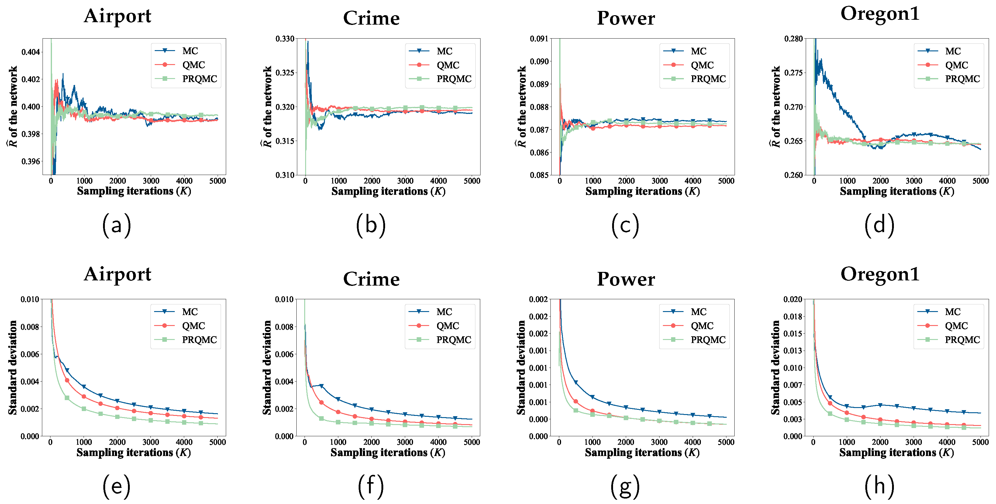
Figure 6 and
Figure 7 present the comparison of the convergence and error between PRQMC and baselines. The figure clearly illustrates that PRQMC achieves faster convergence and better accuracy with fewer samples compared to the baselines.
Additionally,
Table 2 presents a comparison of the computational efficiency of PRQMC and the baselines, each with 5000 sampling iterations. In the PRQMC method, the number of parallel computing processes is set based on the network size, assigning 25 processes to the Karate and Krebs, and 100 processes to the other networks. The results in
Table 2 indicate that the PRQMC method outperforms in terms of computational efficiency. Specifically, the PRQMC method operates nearly 50 times faster than the QMC and MC methods on the Oregon1.
4.3. Comparison of the HBnnsAGP with Baselines
In this subsection, we will demonstrate the effectiveness and efficiency of the proposed HBnnsAGP attack strategy. Specifically, we will compare HBnnsAGP with HDA, HBA, and FINDER on six real-world complex networks, while considering different ASR conditions. Initially, we will employ various attack strategies to generate corresponding attack sequences. Subsequently, we will utilize the PRQMC method to calculate the value under the following ASR distribution scenarios.
ASR = 100%: The ASR of each node is set to 100%.
ASR = 50%: The ASR of each node is set to 50%.
ASR = 50% for the first 30% of nodes: In the attack sequence generated by different attack strategies, the ASR of the first 30% of nodes is set to 50%.
Random ASR: The ASR of each node is randomly set between 50% and 100%. To obtain more reliable results, the average of 10 experimental outcomes is taken.
The sample numbers (
and
) for different networks used in HBnnsAGP are presented in
Table 3.
Table 4 presents the
values of networks in the four specified scenarios. The data suggests that HBnnsAGP performs better than other attack strategies in terms of destructiveness. The destructiveness of HBnnsAGP, on average, has increased by 6.76%, 4.03%, and 7.26% in comparison to the FINDER, HBA, and HDA strategies, respectively.
Table 5 presents a comparison of computation times for HBnnsAGP and the baselines. As the network size increases, the computation time for the HBA method becomes excessively long. In contrast, the HBnnsAGP method maintains commendable computational efficiency even for larger-scale networks. For the Oregon1 network, HBnnsAGP is approximately 28 times faster than HBA. While the computational efficiency of HBnnsAGP slightly lags behind that of FINDER and HDA for larger-scale networks, it surpasses them in terms of attack destructiveness.
Figure 8 represents the ANCw curves of the networks under various attack strategies when the ASR of each node is set to 100%. In this scenario, the state of the attack sequence is unique. The figure shows that HBnnsAGP excels at identifying critical nodes in the network, leading to the effective disruption of the network structure compared to other methods. Hence the effectiveness of the proposed HBnnsAGP attack strategy is verified.
4.4. Further Discussions About Network Robustness
The data presented in
Table 4 indicates that reducing the ASR can significantly enhance network robustness. Generally, this reduction can be achieved through reinforcing node protection. Comparing Scenario 2 and Scenario 3, it is apparent that simply reducing the ASR of the first 30% nodes in the attack sequence (Scenario 3) effectively enhances network robustness. This improvement is approximately 78.25% of that in Scenario 2. Therefore, enhancing the protection of a small subset of crucial nodes in the network can effectively enhance its robustness.
Figure 1.
An example of network disintegration process under different ASR. Gray nodes indicate successful attacks, green nodes represent unsuccessful attacks, and blue nodes denote unattacked nodes.
Figure 1.
An example of network disintegration process under different ASR. Gray nodes indicate successful attacks, green nodes represent unsuccessful attacks, and blue nodes denote unattacked nodes.
Figure 2.
An example of MC integration method for approximating a definite integral over a one-dimensional unit interval. (a) illustrates the approximation of the integral by summing the areas of bars that correspond to the sampled points. Each bar’s height represents the value of at and its width is , where K denotes the total number of samples. (b) demonstrates the sequential rearrangement of the bars to prevent overlapping on the X-axis, ensuring a clear visualization of the areas.
Figure 3.
A comparison of MC and QMC integration methods. (a) and (d) show the two-dimensional projections of a PRS and an LDS (a Sobol sequence) respectively. (b) and (c) depict the MC integration for approximating a definite integral over a one-dimensional unit interval, while (e) and (f) present the QMC integration for approximating a definite integral over a one-dimensional unit interval.
Figure 4.
An example to illustrate the division of the unit hypercube, where and . The unit hypercube is divided into 4 regions, namely , where each region corresponds to a state of , denoted by .
Figure 4.
An example to illustrate the division of the unit hypercube, where and . The unit hypercube is divided into 4 regions, namely , where each region corresponds to a state of , denoted by .
Figure 5.
An illustrative example of non-central nodes and comparison of BC and BCnns. In this figure, (a) highlights non-central nodes in red, (b) showcases node sizes based on BC, and (c) showcases node sizes based on BCnns.
Figure 5.
An illustrative example of non-central nodes and comparison of BC and BCnns. In this figure, (a) highlights non-central nodes in red, (b) showcases node sizes based on BC, and (c) showcases node sizes based on BCnns.
Figure 6.
Comparison of the convergence and error of the PRQMC, QMC, and MC methods in assessing robustness for two smaller-scale networks.
Figure 6.
Comparison of the convergence and error of the PRQMC, QMC, and MC methods in assessing robustness for two smaller-scale networks.
Figure 7.
Comparison of the convergence and standard deviation of the PRQMC, QMC, and MC methods in assessing robustness for four larger-scale networks.
Figure 7.
Comparison of the convergence and standard deviation of the PRQMC, QMC, and MC methods in assessing robustness for four larger-scale networks.
Figure 8.
The ANCw curves of networks under different attack strategies.
Figure 8.
The ANCw curves of networks under different attack strategies.
Table 1.
Basic Information of 6 Real-World Networks. N and M Represent the Number of Nodes and Edges, Respectively, and Denotes the Average Degree of the Network.
Table 1.
Basic Information of 6 Real-World Networks. N and M Represent the Number of Nodes and Edges, Respectively, and Denotes the Average Degree of the Network.
| Network |
Description |
N |
M |
|
| Karate [44] |
Karate club network |
34 |
78 |
4.59 |
| Krebs [10] |
Terrorist network |
62 |
159 |
5.13 |
| Airport [45] |
Aviation network |
332 |
2126 |
12.81 |
| Crime [46] |
Criminal network |
829 |
1473 |
3.55 |
| Power [47] |
Power grid |
4941 |
6594 |
2.67 |
| Oregon1 [48] |
AS peering network |
10670 |
22002 |
4.12 |
Table 2.
Computational Time Comparison of PRQMC, QMC, and MC Methods(s)
Table 2.
Computational Time Comparison of PRQMC, QMC, and MC Methods(s)
| Network |
MC |
QMC |
PRQMC |
| Karate |
1.8 |
1.7 |
0.4 |
| Krebs |
4.5 |
4.3 |
0.6 |
| Airport |
106.7 |
104.9 |
3.0 |
| Crime |
518.2 |
520.6 |
7.4 |
| Power |
20,525.7 |
20,529.1 |
343.7 |
| Oregon1 |
213,748.2 |
213,758.1 |
4,262.4 |
Table 3.
The Sample Numbers ( and ) for Different Networks Used in HBnnsAGP
Table 3.
The Sample Numbers ( and ) for Different Networks Used in HBnnsAGP
| Network |
|
|
| Karate |
16 |
8 |
| Krebs |
30 |
16 |
| Airport |
100 |
60 |
| Crime |
120 |
80 |
| Power |
1300 |
80 |
| Oregon1 |
2300 |
80 |
Table 4.
The Robustness of Networks Under Different ASR. All Values Are Multiplied by 100
Table 4.
The Robustness of Networks Under Different ASR. All Values Are Multiplied by 100
| Network |
HBnnsAGP |
FINDER |
HBA |
HDA |
| 1. ASR=100% |
| Karate |
12.77 |
14.12 |
15.04 |
15.04 |
| Krebs |
12.26 |
16.26 |
14.21 |
17.23 |
| Airport |
7.53 |
10.25 |
7.93 |
11.10 |
| Crime |
9.90 |
11.04 |
10.14 |
11.54 |
| Power |
0.91 |
5.02 |
1.01 |
5.23 |
| Oregon1 |
0.68 |
1.06 |
0.73 |
1.01 |
| Avg score |
7.34 |
9.63 |
8.18 |
10.19 |
| 2. ASR=50% |
| Karate |
59.90 |
60.55 |
60.88 |
61.41 |
| Krebs |
57.61 |
58.38 |
57.74 |
58.33 |
| Airport |
59.45 |
60.32 |
60.39 |
60.52 |
| Crime |
57.59 |
59.50 |
59.50 |
59.08 |
| Power |
16.54 |
19.73 |
17.31 |
19.93 |
| Oregon1 |
49.68 |
51.58 |
51.28 |
51.33 |
| Avg score |
50.13 |
51.69 |
51.18 |
51.77 |
| 3. ASR = 50% for the first 30% of nodes |
| Karate |
48.61 |
50.38 |
49.76 |
50.57 |
| Krebs |
45.51 |
47.16 |
45.78 |
47.38 |
| Airport |
48.78 |
50.68 |
51.00 |
50.47 |
| Crime |
41.84 |
48.17 |
46.90 |
47.12 |
| Power |
14.87 |
17.79 |
16.32 |
17.86 |
| Oregon1 |
41.26 |
42.91 |
42.83 |
43.14 |
| Avg score |
40.15 |
42.91 |
42.10 |
42.76 |
| 4. Random ASR |
| Karate |
35.12 |
36.29 |
36.50 |
37.57 |
| Krebs |
30.39 |
32.99 |
31.02 |
33.36 |
| Airport |
36.95 |
38.58 |
38.67 |
38.99 |
| Crime |
27.90 |
30.96 |
30.48 |
30.42 |
| Power |
5.17 |
8.46 |
5.18 |
8.80 |
| Oregon1 |
21.61 |
24.23 |
23.52 |
23.86 |
| Avg score |
26.19 |
28.56 |
27.55 |
28.79 |
Table 5.
The Computation Time of Different Attack Strategies(ms)
Table 5.
The Computation Time of Different Attack Strategies(ms)
| Network |
HBnnsAGP |
FINDER |
HBA |
HDA |
| Karate |
1.6 |
16.3 |
1.9 |
0.5 |
| Krebs |
3.6 |
36.6 |
4.6 |
2.3 |
| Airport |
82.3 |
218.3 |
211.0 |
11.1 |
| Crime |
552.1 |
369.3 |
4,434.6 |
49.1 |
| Power |
6,760.7 |
1,397.9 |
78,119.9 |
1,796.8 |
| Oregon1 |
15,799.1 |
8,641.5 |
477,802.8 |
2,065.9 |
