
Submitted:
06 October 2023
Posted:
09 October 2023
You are already at the latest version
Abstract
Energy demand forecasting is a fundamental aspect of modern energy management. It impacts resource planning, economic stability, environmental sustainability, and energy security. This importance is making it critical for countries worldwide, particularly in cases like Türkiye, where the energy dependency ratio is notably high. The goal of this study is to propose ensemble machine learning methods such as boosting, bagging, blending, and stacking with hyperparameter tuning and k-fold cross-validation, and investigate the application of these methods for predicting Türkiye's energy demand. This study utilizes population, GDP per capita, imports and exports as input parameters based on historical data from 1979 to 2021 in Türkiye. Eleven combinations of all predictor variables were analyzed, and the best one was selected. It was observed that a very high correlation exists among population, GDP, imports, exports, and energy demand. In the first phase, the preliminary performance was investigated of 19 different machine learning algorithms using 5-fold cross-validation and measured their performance using five different metrics: MSE, RMSE, MAE, R-squared, and MAPE. Secondly, ensemble models were constructed by utilizing individual machine learning algorithms, and the performance of these ensemble models was compared with both each other and the best-performing individual machine learning algorithm. The analysis of the results revealed that placing Ridge as the meta-learner and using ET, RF and Ridge as the base learners in the stacking ensemble model produced superior results compared to the other models across performance metrics. It is anticipated that the findings of this research can be applied globally and prove valuable for energy policy planning in any country. The results obtained not only highlight the accuracy and effectiveness of our predictive model but also underscore the broader implications of this study within the framework of the United Nations' Sustainable Development Goals (SDGs).
Keywords:
energy demand
; ensemble machine learning
; SDG’s
; Türkiye
1. Introduction
Energy plays a vital role in supporting social and economic development of a country from past to present. It drives economic growth, improves living standards, supports social services, enhances national security, and contributes to environmental sustainability. Ensuring reliable, affordable, and sustainable energy access is essential for a country's overall development and progress. Therefore, the development of energy policies and the estimation of energy demand are a most important priority for developed and developing countries. Türkiye is the 19th largest economy in the world, with a gross domestic product (GDP) of roughly $906 billion [1]. Therefore, as a fast-growing economy, Türkiye's energy consumption has undergone significant growth and diversification over the years. As a rapidly developing country, Türkiye has experienced a substantial increase in energy demand due to population growth, urbanization, industrialization, and economic expansion. In terms of energy sources, Türkiye has a mix of fossil fuels, renewable energy, and imports. Electricity consumption constitutes a significant portion of Türkiye's energy consumption. However, the energy production in Türkiye is rather low in spite of the considerable increase in energy consumption.
In 2021, Türkiye produced approximately 41.3 MTOE (million tons of oil equivalent), mostly based on coal and lignite (57.5 %). In contrast, the country's energy consumption reached approximately 109.8 MTOE in the same year. The substantial gap between energy production and consumption led to Türkiye becoming one of the major energy importing countries in Europe [2]. As a report of Ministry of Energy and Natural Resources in September 2021, Türkiye's energy dependency rate was reported to be around 74%. This means that Türkiye relied on imports to meet approximately 74% of its total energy consumption. The country heavily depended on imports of natural gas and oil to bridge the energy gap between domestic production and demand [3].
To provide energy either by importing or by producing, forecasting energy consumption, analyzing the relationship between energy demand and supply are crucial issues in short and long term energy planning. Managing energy demand also involves identifying and prioritizing energy resources, optimizing energy utilization, improving energy efficiency, shaping policy decisions, and devising strategies to reduce emissions.
Furthermore, it is important to emphasize that the United Nations' SDGs provide a comprehensive blueprint for addressing global challenges and promoting sustainability by 2030 [4]. This study aligns closely with several of these goals: including Goal 7, Goal 8, and Goal 13, making a significant contribution to the broader aims of sustainable development. Accurate energy demand forecasting plays a central role in achieving 'Goal 7: Affordable and Clean Energy.' By optimizing energy production, distribution, and consumption, this study facilitates the provision of affordable, reliable, and clean energy. This, in turn, supports economic growth, enhances energy access, and reduces environmental impacts. Moreover, this study directly addresses 'Goal 13: Climate Action' by mitigating the effects of climate change. Through precise energy demand predictions, it empowers Türkiye to make informed decisions that reduce greenhouse gas emissions, promote renewable energy adoption, and foster a low-carbon, sustainable energy sector. Energy efficiency serves as a catalyst for economic growth and job creation, aligning with 'Goal 8: Decent Work and Economic Growth.' This study enables Türkiye to implement energy-efficient measures, leading to cost savings for industries and households.
Researchers have developed various statistical techniques, meta-heuristic algorithms, artificial intelligence techniques in energy modeling. Artificial Neural Networks (ANNs), have gained significant interest in energy planning due to their ability to handle complex nonlinear relationships between input and output data [5]. ANNs have been applied in various energy forecasting applications, including gas consumption [6], energy demand [7], electricity consumption [8], transportation energy demand [9,10,11] energy source analysis [12] and energy dependency [7]. Apart from ANNs, other prediction methods have emerged, such as Fuzzy Logic, Adaptive Network-based Fuzzy Inference System (ANFIS), and general Machine Learning algorithms [13,14,15]. It's important to recognize that Artificial Neural Network (ANN) is a subfield of Machine Learning (ML), which, in itself, is a subset of Artificial Intelligence (AI). Frequently, the terms AI, ML, and Deep Learning (DL) are used interchangeably to refer to intelligent systems or software. DL, specifically, extends the concept of ANNs by incorporating extra hidden layers and employing specialized activation functions that aren't typically found in traditional ANN models.
The AI-based prediction models have received considerable interest to solve a variety of problems in energy planning recently. These models leverage the power of artificial intelligence techniques to forecast future outcomes based on historical data patterns. These models use advanced algorithms and machine learning methods to analyze large datasets, identify patterns, and make predictions.
Research on predicting Türkiye's energy requirements began in the 1960s, with the State Planning Organization (SPO) employing basic regression techniques for energy forecasting. In the late 1970s, The Ministry of Energy and Natural Resources (MENR) and the Turkish Statistical Institute (TSK) started preparing energy demand projections [16], but the estimated values provided by MENR were found to be higher than the actual energy demand [17]. Numerous econometric modeling techniques were applied to forecasting energy consumption after 1984. the Model for Analysis of Energy Demand (MAED) is most frequently used approach developed by MENR [18]. Nevertheless, the energy demand predictions generated by MAED continued to overstate actual demand, rendering them unreliable [19,20]. Utgikar and Scott [21] conducted an inquiry to understand the reasons behind unsuccessful energy predictions. They found that although statistical models are favored by researchers due to their simplicity, they tend to deliver acceptable results only for short-term periods, while becoming increasingly unstable for longer-term forecasts. While statistical models have contributed valuable insights to energy forecasting studies, El-Telbany and El-Karmi [22] argue that these models, which rely on statistical methods, perform well under normal conditions but struggle to account for sudden changes in environmental or sociological variables. Due to the above discussed reasons, researchers have garnered the interest in the field of energy demand modeling.
AI-based prediction methods utilize advanced algorithms and models that learn patterns, relationships, and trends from historical data to make accurate predictions about future events or outcomes. AI-based prediction methods have gained significant popularity due to their ability to handle complex, non-linear relationships and adapt to changing data patterns. Machine Learning (ML) is an AI-based prediction method, which encompasses a range of algorithms that automatically learn and improve from data without being explicitly programmed. Deep Learning (DL), a subset of ML, has emerged as a powerful AI-based prediction method.
AI-based prediction methods have demonstrated their effectiveness in various fields, including finance, healthcare, weather forecasting, sales forecasting, demand prediction, and fraud detection [23,24,25,26]. However, it's important to note that when applying these methods to real-world scenarios, Factors such as data quality, feature selection, model complexity, and interpretability should be carefully considered. Machine learning approaches can be broadly categorized into three main types: supervised learning, unsupervised learning, and reinforcement learning. Supervised learning algorithms include Classification and Regression. The regression is used for energy demand in this work. In machine learning, ensemble learning and deep learning methods outperform traditional algorithms. Ensemble methods are learning algorithms that build a set of classifiers and then classify new data points by taking (weighted) votes of their predictions. The effectiveness of an ensemble method depends on several factors, including how the underlying models are trained and how they are combined. In the literature, there are common approaches to building ensemble models that have been successfully demonstrated in various domains [27,28,29].
Ensemble machine learning is a powerful technique in the field of machine learning that involves combining the predictions of multiple individual models (base models) to create a more accurate and robust predictive model. This approach, preferred over single methods, offers several key advantages. Firstly, ensembles enhance prediction accuracy by aggregating multiple models, reducing errors, and biases. Secondly, they mitigate overfitting, a common issue in machine learning, by balancing out individual model weaknesses. Moreover, ensembles prove their robustness by effectively handling noisy data and outliers, making them suitable for real-world applications [30]. In automated decision-making applications, especially in engineering, ensemble methods have demonstrated superior performance compared to individual learners. This is attributed to their ability to capture diverse patterns, reduce bias and variance, and improve generalization. Ensemble methods are particularly effective when there is a large amount of data, complex relationships, and a need for high predictive accuracy.
Common ensemble method strategies comprise bagging, boosting, blending, and stacking. Bagging, exemplified by the Random Forest algorithm, enhances model robustness by reducing overfitting and improving prediction accuracy through the wisdom of the crowd [31]. Boosting is another ensemble technique that iteratively builds a strong predictive model by giving more weight to the data points that previous models misclassified [32]. Bagging reduces variance by averaging over multiple models, boosting focuses on reducing bias through weighted data points. Blending, sometimes referred to as model stacking or meta-ensembling, involves training multiple diverse base models on the same dataset and then combining their predictions using a separate model trained on the validation set. Stacking, similar to blending, combines multiple base models to form a meta-model but differs in its approach. In stacking, the predictions of the base models serve as input features for a meta-model, which learns to make the final predictions [33]. Blending combines diverse models with a separate meta-model, and stacking uses base models to create a meta-model for predictions. The choice among these ensemble methods depends on the specific problem, dataset, and the trade-off between bias and variance in the model [34].
The main objective of this study is to use ensemble machine learning methodologies, which have not received much attention in prior research on energy, to assess energy demand in Türkiye. In this paper, several significant contributions were presented, including empirical evidence substantiating the efficacy of ensemble methods in forecasting Türkiye's energy demand, comprehensive hyperparameter tuning, and an exhaustive examination of 19 distinct machine learning algorithms along with the application of 5 performance metrics to evaluate their predictive capabilities. To the best of our knowledge, this paper is the first to investigate Türkiye's energy demand using ensemble machine learning models.
This paper is organized as follows: Section 2 will provide an overview of the scope and definition of energy demand studies. Section 3 will present the primary methods and approaches employed in energy demand study, along with the main data sources and challenges associated with energy. In Section 4, the principal findings and trends will be discussed using various ensemble learning algorithms. Section 5 will summarize the main implications and recommendations from the results of energy demand study. Finally, our paper will conclude with a discussion of limitations and directions for future research.
2. Literature Review
Energy demand forecasting is an important task for planning and managing energy systems. It involves predicting the future energy consumption of different sectors, regions, or appliances based on various factors such as weather, economic activity, population, lifestyle, etc. This literature review aims to summarize some of the key findings and trends from recent articles on this topic.
2.1. Review of Energy Demand Forecasting in the World
The global energy crisis of 2022 has brought renewed attention to the challenges and opportunities of energy demand in a rapidly changing world. According to various sources, such as the World Energy Outlook 2022 by the International Energy Agency (IEA), the Outlook for Energy Demand by McKinsey, and several articles from reputable media outlets, energy demand is undergoing a major transformation due to a combination of factors, such as economic slowdown, high energy prices, energy security concerns, and climate policies.
The global energy demand has been affected by the Covid-19 pandemic and the economic recovery in 2021. According to the Global Energy Review 2021 by the International Energy Agency (IEA), the global energy demand is expected to grow by 4.6% in 2021. The IEA projects that global energy demand will grow by 0.8% per year on average between 2021 and 2030 in its Stated Policies Scenario (STEPS), which reflects current and announced policies and targets [35]. This literature review has provided a brief overview of some of the main findings and trends from recent articles on energy demand.
There are many methods for energy demand forecasting, spanning from conventional approaches like econometric and time series models to contemporary soft computing techniques, including artificial intelligence methods and heuristics.
Zhang et al. [36] aimed to predict the transport energy demand in China for the next two decades using a statistical method called partial least square regression (PLSR). The study estimated that by 2020, China would need about 433 to 468 million tons of coal equivalent (Mtce) of energy for its transportation sector, mainly from petroleum products. The study demonstrated the usefulness of PLSR as a simple and reliable technique for forecasting transport energy demand.
Kumar and Jain [37] presented three time series models for forecasting the consumption of conventional energy in India. The study assessed the accuracy of these forecasts by comparing them with both actual data and projections made by the Planning Commission of India.
Chaturvedi et al. [38] evaluated four time-series models for predicting total and peak monthly energy demand in India. The study compared the performance of the Seasonal Auto-Regressive Integrated Moving Average (SARIMA), Long Short Term Memory Recurrent Neural Network (LSTM RNN), and Facebook Prophet (Fb Prophet) models in forecasting Indian energy demand. Among these models, Fb Prophet performed well for both total and peak demand, exhibiting lower prediction errors compared to the others.
Sahraei et al. [39] presented the transportation energy demand in Türkiye using a statistical method called Multivariate Adaptive Regression Splines (MARS), which is a nonparametric regression technique. They established five models and compared with real data which are collected from MENR. The approach employed in that study illustrates the utility of the MARS method in examining and forecasting energy consumption within the transportation sector.
Machine learning algorithms have been applied to predict energy consumption in various studies. Javanmard and Ghaderi [40] studied about predicting energy demand in Iran until 2040 using machine learning and optimization algorithms. The authors collect data from different energy sectors and apply six machine learning algorithms (ARIMA, SARIMA, SARIMAX, ANN, AR, and LSTM) and mathematical programming to forecast the energy demand. Then, they use an integrated model with Particle Swarm and Grey-Wolf optimization algorithms to improve the prediction accuracy. They compare the results of the proposed method with the machine learning algorithms and report a high accuracy for the proposed method. The study also estimated the growth rate of energy demand in each sector.
Ye et al. [41] employed the discrete grey model (DGM) to enhance the accuracy of energy consumption predictions. Meanwhile, Zhang and Wang [42] introduced a fuzzy wavelet neural network (FWNN) method to forecast annual electricity consumption in a city known for its high energy consumption in China.
El-Telbany and El-Karmi [22] presented and discussed the results of applying ANN to forecast the energy demand using PSO method, which was a novel adaptive algorithm based on a social-psychological metaphor. They compared the performance of this method with the performance of BP algorithm and autoregressive moving average technique.
Mason et al. [43] utilized the covariance matrix adaptation evolutionary strategy, a powerful evolutionary optimization algorithm, to train neural networks for predicting Ireland's energy needs. The neural network trained with the covariance matrix adaptation evolutionary strategy performed well compared to other state-of-the-art prediction methods.
Muratlıharan et al. [44] introduced a novel approach for energy demand prediction by utilizing neural networks in an optimization framework. Initially, the Conventional Neural Network (CNN) approach was employed to predict energy demand at the consumer level. Then, two variations, namely the Neural Network based Genetic Algorithm (NNGA) and Neural Network based Particle Swarm Optimization (NNPSO), were proposed to automatically adjust the neural network weights. The results indicated that the NNGA approach outperforms in short-term load forecasting, while the NNPSO approach is more suitable for long-term energy prediction.
Yu et al. [45] introduced a hybrid algorithm known as the Particle Swarm Optimization and Genetic Algorithm Optimal Energy Demand Estimating (PSO–GA EDE) model to estimate China's energy demand. Their study demonstrated the superiority of this model when compared to alternative approaches.
In general, statistical technique and artificial intelligence can be used for solving the real-world problems. Statistical techniques involve mathematical models, including regression, multiple regression models, Autoregressive Moving Average, and Kalman filters [39,41]. Evolutionary algorithms, such as genetic algorithms and particle swarm optimization, are also employed. Artificial intelligence approaches involve a combination of fuzzy logic, artificial neural networks, genetic algorithms, support vector machines, and machine learning methods [46].
A systematic literature review encompassing 419 articles on energy demand modeling, covering the period between 2015 and 2020, was conducted by Verwiebe et al. [46]. They analyzed the methodologies, prediction accuracy, input variables, energy sources, sectors, temporal scopes, and spatial resolutions employed in these models. They found that machine learning techniques were the most used, followed by engineering-based models, metaheuristic and uncertainty techniques, and statistical techniques. They also discussed the drawbacks and countermeasures of each technique. Another systematic literature review of energy demand forecasting methods published in 2005–2015 was conducted by Ghalehkhondabi et al. [47]. They focused on the methods that are used to predict energy consumption and compared their performance and applicability. They reported that neural networks were the most cited technique and had notable performance, but also high computation time. They suggested that hybrid methods could be a promising field of future research.
2.2. Energy Demand Forecasting in Türkiye
A summary of studies for the Türkiye's energy demand forecasting is tabulated in Table 1. However, to the best of our knowledge, there is no research paper that employs ensemble machine learning methods and compares them with each other to forecast Türkiye's energy demand.
3. Materials and Methods
In this section, proposed methodology is introduced in detail. Ensemble methods refer to algorithms that combine multiple machine learning models into a unified framework. These methods have gained significant attention and recognition in the machine learning community due to their ability to enhance prediction accuracy and robustness [41,42]. By combining the predictions of multiple models, ensemble methods can mitigate the limitations of individual models and provide more accurate and reliable results. Several types of ensemble methods commonly used in machine learning are Bagging, Boosting, Blending, Random Forest and Stacking [31,32,33,34]. This paper proposes and analyzes different ensemble combination models that can be achieved by using diverse base models, varying model architectures, or training on different subsets of the data.
3.1. ML Algorithms
In the context of forecasting Türkiye's energy demand, 19 machine learning algorithms have been selected that have demonstrated excellent performance in energy consumption forecasting problems. These algorithms are briefly described below.
- Light Gradient Boosting Machine (LightGBM) [72]
LightGBM is a popular machine learning algorithm used for both regression and classification tasks. It is designed to efficiently handle large-scale datasets with high-dimensional features. LightGBM is known for its speed, accuracy, and ability to handle complex problems. LightGBM is based on the gradient boosting framework, similar to other boosting algorithms. However, it incorporates several optimizations that make it more efficient and scalable. One key optimization is the implementation of a novel histogram-based algorithm for binning and feature discretization. This approach reduces the memory usage and speeds up the training process by avoiding the need to sort data during each iteration. Another important feature of LightGBM is the implementation of a leaf-wise tree growth strategy. Unlike traditional depth-wise growth, where trees are expanded level by level, LightGBM grows trees’ leaf by leaf. This approach reduces the number of levels in the trees, resulting in faster training and improved accuracy.
- XGBoost [73]
XGBoost Regressor is a powerful machine learning algorithm used for regression tasks. XGBoost Regressor is known for its efficiency, accuracy, and ability to handle complex datasets. The algorithm minimizes a loss function by iteratively adding decision trees to the ensemble. Each tree is trained to predict the residuals (the differences between the actual and predicted values) of the previous ensemble. The process continues until a specified number of trees is reached or the desired level of performance is achieved. To further improve the performance, XGBoost Regressor incorporates several advanced techniques. It employs a regularization term in the objective function to control the complexity of the model and prevent overfitting. It uses a technique called gradient boosting with shrinkage, which adds a weighting factor to each tree's contribution, allowing for more conservative updates.
XGBoost Regressor offers several advantages. It is highly customizable, allowing users to fine-tune various hyperparameters to achieve optimal performance. It can handle large-scale datasets with a high number of features and is computationally efficient due to parallelization and tree pruning techniques.
- Extra Tree Regression [74]
Extra Trees Regression is a machine learning algorithm used for regression tasks. It belongs to the ensemble learning family and is an extension of the popular Random Forest algorithm. Extra Trees Regression combines multiple decision trees to make predictions by aggregating their outputs. The algorithm builds a user-defined number of decision trees using random subsets of the training data and random subsets of features. Each tree is grown to its maximum depth, resulting in a collection of unpruned and highly random trees. The final prediction is then obtained by averaging or aggregating the predictions made by each tree.
Extra Trees Regression offers several advantages. First, it reduces overfitting since the randomization helps to capture different aspects of the data. It can handle high-dimensional datasets with a large number of features and works well with both continuous and categorical variables. Additionally, it is computationally efficient as the trees can be grown in parallel.
- Passive Aggressive Regressor (PAR) [75]
(PAR) is a machine learning algorithm used for regression tasks. In Passive Aggressive Regressor, the algorithm updates the regression model incrementally, making predictions on new instances as they arrive. It adapts to new data points by adjusting the model's parameters without revisiting the entire training set. This property makes it suitable for handling large-scale datasets or scenarios where data arrives in a streaming fashion.
Passive Aggressive Regressor is particularly useful when dealing with dynamic or non-stationary data, as it can update the model in an online fashion. It is also memory-efficient since it does not require storing the entire training set.
- Elastic Net [76]
Elastic Net is a regression method that combines the Lasso and Ridge regression techniques. It is used for feature selection and regularization in linear models, providing a balance between the two methods. In Elastic Net, the algorithm aims to minimize the sum of squared residuals between the predicted and actual values, similar to ordinary least squares (OLS) regression. However, Elastic Net adds a penalty term to the cost function that combines both the Lasso (L1) and Ridge (L2) penalties. The penalty term is a linear combination of the absolute values of the coefficients (L1) and the squared values of the coefficients (L2), each multiplied by their respective tuning parameters. The combination of L1 and L2 penalties in Elastic Net allows for both feature selection and regularization.
- Least Angle Regression (LARS) [77]
LARS is a regression method used for feature selection and model building. It is an algorithm that selects predictors in a direction that minimizes the prediction error and correlates strongly with the target variable. LARS starts with an empty set of selected features and gradually adds features in a way that balances their correlations and coefficients. In each iteration, LARS identifies the most correlated feature with the residual and increases the coefficient of that feature along its equiangular direction. The algorithm continues this process until it reaches the desired number of selected features or the maximum number of available features.
- Lasso Least Angle Regression [78]
Lasso Least Angle Regression is a regression method that combines the features of the Lasso regularization and the Least Angle Regression algorithm. It is used for feature selection and regularization in linear regression tasks. Lasso Least Angle Regression aims to estimate the coefficients of a linear regression model while simultaneously performing feature selection by encouraging sparsity in the solution. It starts with an empty set of selected features and gradually adds features in a way that balances their correlations and coefficients.
This algorithm provides a continuous path of solutions for different regularization levels, allowing for more flexibility in choosing the amount of regularization. It is particularly useful when dealing with high-dimensional datasets where feature selection and regularization are crucial to prevent overfitting and improve interpretability.
- Orthogonal Matching Pursuit (OMP) [79]
Orthogonal Matching Pursuit (OMP) is an algorithm used for sparse signal recovery and feature selection tasks. It aims to find the most relevant features or components of a signal by iteratively selecting and reconstructing the signal based on a small subset of measurements or features. In OMP, the algorithm starts with an initial guess of the solution and iteratively improves it by selecting the most correlated features with the residual error. In each iteration, the algorithm identifies the feature that has the highest correlation with the residual and adds it to the solution. It then updates the residual by subtracting the contribution of the selected feature from the original signal. This process continues until a predefined stopping criterion is met, such as a desired level of approximation or a fixed number of selected features.
OMP leverages the orthogonality property to efficiently select features and estimate the signal. At each iteration, the algorithm ensures that the selected features are orthogonal or nearly orthogonal to each other, which helps in accurate signal reconstruction and efficient convergence.
- Random Forest Regressor [80]
Random Forest Regressor is a popular machine learning algorithm used for regression tasks. It belongs to the ensemble learning family and is built upon the concept of decision trees. In Random Forest Regressor, a user-defined number of decision trees are constructed. Each tree is built using a random subset of the training data and a random subset of features. The process of constructing each tree involves recursively splitting the data based on different features and their respective splitting points. The splitting is done in a way that minimizes the variance of the target variable within each resulting subset. During prediction, each tree in the random forest independently generates a prediction. The final prediction is obtained by averaging or taking the majority vote (in the case of classification) of the predictions from all the trees.
Random Forest Regressor offers several advantages. It can handle high-dimensional datasets with a large number of features and works well with both continuous and categorical variables. Additionally, it provides a measure of feature importance, allowing for better understanding of the underlying relationships in the data.
- Gradient Boosting Regressor [81]
Gradient Boosting Regressor is a powerful machine learning algorithm used for regression tasks. It belongs to the boosting family of algorithms and is designed to create a strong learner by iteratively combining weak learners. Gradient Boosting Regressor works by minimizing a loss function through an additive approach, where each new model is built to correct the errors made by the previous models. In Gradient Boosting Regressor, the algorithm starts by creating an initial model, often a simple one like a decision tree. This model makes initial predictions on the training data. The subsequent models are then built to minimize the differences between the predicted and actual values of the previous models. The new models are trained on the negative gradients of the loss function with respect to the previous ensemble's predictions. This means the new models learn to predict the residuals or errors made by the existing ensemble. The final prediction is obtained by aggregating the predictions from all the models in the ensemble.
Gradient Boosting Regressor offers several advantages. It can handle complex datasets and capture intricate relationships between features. It is also capable of handling various loss functions, making it adaptable to different regression problems. The algorithm is robust against overfitting due to regularization techniques employed during the training process.
- AdaBoost Regressor [82]
AdaBoost Regressor, short for Adaptive Boosting Regressor, is a machine learning algorithm used for regression tasks. The algorithm iteratively trains a series of weak regressors, each focusing on the instances that were mis predicted by the previous regressors, to improve the overall prediction accuracy. In AdaBoost Regressor, each weak regressor is trained on a subset of the training data. During training, the algorithm assigns weights to each instance, with initially equal weights for all instances. In each iteration, a weak regressor is trained on the weighted training data, and the weights are adjusted based on the performance of the regressor. Instances that are mispredicted by the current regressor are given higher weights, while correctly predicted instances are given lower weights. This emphasizes the importance of the mispredicted instances in subsequent iterations. During prediction, the weak regressors are combined by assigning weights to their predictions. The final prediction is obtained by aggregating the weighted predictions of all the weak regressors. The weights are determined based on the performance of each regressor during training. The regressors with better performance are given higher weights, indicating their greater influence on the final prediction. AdaBoost Regressor has several advantages. It can handle complex relationships in the data and is resistant to overfitting. By focusing on mispredicted instances, it iteratively improves the model's ability to capture difficult patterns in the data.
- Linear Regression [83]
Linear regression is a statistical method that models the relationship between a dependent variable (y) and one or more independent variables (x). It can be used to estimate how the dependent variable changes as the independent variables change, and to test hypotheses about the strength and direction of the relationship. There are different types of linear regression, such as simple linear regression (one independent variable), multiple linear regression (more than one independent variable), and multivariate linear regression (more than one dependent variable). Linear Regression is a widely used statistical modeling method for predicting a continuous target variable based on one or more predictor variables. It assumes a linear relationship between the predictors and the target variable, where the goal is to find the best-fitting line or hyperplane that minimizes the difference between the predicted and actual values.
- Lasso Regression [84]
Lasso Regression (LASSO) is a method of regression analysis that performs both variable selection and regularization. It aims to improve the prediction accuracy and interpretability of the regression model by shrinking the coefficients of some predictor variables to zero and reducing the magnitude of others.
In Lasso Regression, the algorithm aims to minimize the sum of squared residuals between the predicted and actual values, similar to ordinary least squares (OLS) regression. However, Lasso Regression adds a penalty term to the cost function, known as the Lasso or L1 penalty. This penalty term is the sum of the absolute values of the coefficients multiplied by a tuning parameter called the regularization parameter or lambda (λ).
- K Neighbors Regressor [85]
K Neighbors Regressor is a machine learning algorithm used for regression tasks. It is a non-parametric method that predicts the target value of an instance by considering the average or weighted average of the target values of its k nearest neighbors in the training data. In K Neighbors Regressor, the algorithm identifies the k nearest neighbors of a given instance based on a distance metric, such as Euclidean distance. The target values of these neighbors are then used to calculate the predicted value for the instance. In the case of average-based prediction, the predicted value is the average of the target values of the k neighbors. In the case of weighted average prediction, the predicted value is the weighted average, where the weights are determined based on the proximity of the neighbors to the instance. The value of k in K Neighbors Regressor determines the number of neighbors to consider in the prediction.
K Neighbors Regressor offers simplicity and flexibility. It can handle both numerical and categorical features and can capture complex relationships in the data.
- Bayesian Ridge Regression [86]
Bayesian Ridge Regression is a regression method that incorporates Bayesian principles into the linear regression framework. In Bayesian Ridge Regression, the algorithm places a prior distribution on the regression coefficients, typically assuming a Gaussian distribution. This prior distribution represents the initial belief about the likely values of the coefficients before observing the data. As data is observed, the prior distribution is updated to form the posterior distribution, which represents the updated belief about the coefficient values given the observed data.
The posterior distribution is obtained using Bayes' theorem, which combines the prior distribution with the likelihood function of the data. The likelihood function expresses the probability of observing the data given the regression coefficients. The posterior distribution captures the uncertainty in the coefficient estimates and can be used to compute credible intervals or conduct hypothesis tests.
- Decision Tree Regressor [87]
Decision Tree Regressor is a machine learning algorithm used for regression tasks. It is based on the concept of a decision tree, which partitions the input space into regions and predicts the target value based on the average or majority value of the training instances within each region. In Decision Tree Regressor, the algorithm recursively splits the data based on different features and their respective splitting points to create a tree-like structure. The splitting is done in a way that minimizes the variance or mean squared error of the target variable within each resulting subset. Each internal node of the tree represents a splitting point, and each leaf node represents a prediction for a subset of data.
Decision Tree Regressor offers several advantages. It is intuitive and easy to interpret, as the resulting tree structure can be visualized and understood. It can handle both numerical and categorical features and can capture complex nonlinear relationships in the data. Decision Tree Regressor is also robust to outliers and can handle missing values in the data.
- Ridge Regression [88]
Ridge Regression is a linear regression method used for modeling and prediction tasks. It is an extension of ordinary least squares (OLS) regression that introduces a regularization term to handle multicollinearity and prevent overfitting. In Ridge Regression, the algorithm seeks to minimize the sum of squared residuals between the predicted and actual values, similar to OLS regression. However, Ridge Regression adds a penalty term, known as the Ridge or L2 penalty, to the cost function. This penalty term is the squared sum of the coefficients multiplied by a tuning parameter called the regularization parameter or lambda (λ). The regularization parameter (λ) controls the degree of shrinkage applied to the coefficients. A larger λ value increases the amount of shrinkage, resulting in a more heavily regularized model with smaller coefficient values. Conversely, a smaller λ value reduces the amount of shrinkage, making the model behave more like ordinary least squares regression.
Ridge Regression offers several advantages. It is particularly useful when dealing with multicollinearity, where the predictor variables are highly correlated. It also provides a balance between bias and variance, helping to prevent overfitting in situations where the number of predictors is larger than the number of observations.
- Huber Regressor [89]
Huber Regressor is a robust regression method that combines the benefits of both least squares’ regression and robust regression techniques. Huber Regressor addresses these issues by introducing a hybrid loss function that behaves like least squares for small residuals and like a scaled absolute loss for large residuals. The loss function is controlled by a tuning parameter called the Huber loss threshold. Residuals below the threshold are squared, while residuals above the threshold are linearly scaled. This combination of squared and absolute loss enables Huber Regressor to provide a balance between robustness to outliers and accuracy for non-outlying data points. During training, Huber Regressor estimates the coefficients of the linear regression model by minimizing the modified loss function. This estimation process reduces the influence of outliers while still accurately capturing the patterns in the majority of the data.
- Dummy Regressor
Dummy Regressor is a simple baseline model used for regression tasks. It provides a straightforward way to establish a baseline performance against which other regression models can be compared. Dummy Regressor makes predictions based on simple rules or heuristics rather than learning patterns from the data. In Dummy Regressor, the predictions are determined based on a predefined strategy.
The Materials and Methods should be described with sufficient details to allow others to replicate and build on the published results. Please note that the publication of your manuscript implicates that you must make all materials, data, computer code, and protocols associated with the publication available to readers. Please disclose at the submission stage any restrictions on the availability of materials or information. New methods and protocols should be described in detail while well-established methods can be briefly described and appropriately cited.
Research manuscripts reporting large datasets that are deposited in a publicly available database should specify where the data have been deposited and provide the relevant accession numbers. If the accession numbers have not yet been obtained at the time of submission, please state that they will be provided during review. They must be provided prior to publication.
Interventionary studies involving animals or humans, and other studies that require ethical approval, must list the authority that provided approval and the corresponding ethical approval code.
3.2. Structure of the Proposed Methods
This section presents the structure and abstract overview of the study, with a basic conceptual flow shown in Figure 1. The methodology consists of several key steps to improve the accuracy of our models. The first step entails data preparation, encompassing data preprocessing, normalization, and transformation to ensure the dataset is primed for analysis. Following this, the performance of 19 different machine learning algorithms have been assesed. This evaluation forms the basis for creating various ensemble combinations that leverage the strengths of individual models. In the third step, four different ensemble techniques like bagging, boosting, blending, and stacking models have been used to to create powerful ensemble models that can capture complex patterns and relationships in the data. Finally, our study concludes with the fourth step, where it has carefully evaluated and compared these ensemble models, gaining insights into their strengths and weaknesses. This comprehensive evaluation process has informed our final prediction, guiding us towards data-driven decisions that hold the potential to advance the field of artificial intelligence and machine learning.
3.2.1. K-Fold Cross-Validation
The next step in the processing block involves selecting machine learning algorithms that exhibit superior performance and diverse learning capabilities when applied to our energy dataset. K-fold cross-validation is a technique used in machine learning algorithms to evaluate the performance of a model by dividing the available data into k equally sized subsets or "folds." The process entails iteratively training the model on k-1 folds and then evaluating it on the remaining fold. This cycle is repeated k times, with each fold being used as the test set exactly once. The final evaluation is obtained by averaging the performance results from each iteration. The value of k is usually chosen as k=5 or k=10. A 5-fold cross-validation is used to obtain groups of performance measures in this study. By using different subsets of data for training and validation, k-fold cross-validation helps to assess the model's ability to generalize well to unseen data. This process helps to mitigate issues such as overfitting and provides a more reliable estimate of our model's performance by averaging the results obtained from each iteration.
3.2.2. Model Hyperparameters Tuning
Hyperparameter tuning is the process of finding the optimal values for the hyperparameters of a machine learning algorithm. Hyperparameters are parameters that are set before the learning process begins and determine how the algorithm learns and generalizes from the training data. By selecting the right combination of hyperparameter values, we can improve the model's accuracy, generalization, and robustness [90].
In this study, hyperparameter tuning was employed to improve model performance and prevent overfitting before proceeding to the next stage of our framework. The commonly used approaches for hyperparameter tuning are Grid Search, Random Search, and Bayesian Optimization. Grid search involves defining a grid of hyperparameter values and searching through a predefined set of hyperparameter values for a given model. In random search, hyperparameters are randomly sampled from predefined distributions. Bayesian optimization uses probabilistic models to estimate the performance of different hyperparameter configurations. The choice of the technique ultimately depends on the specific problem, available computational resources, and the characteristics of the hyperparameter search space. In this work Grid Search approach has used.
3.2.3. Performance Metrics
The performance of ML algorithms in our energy demand problem was estimated using powerful validation techniques. Five validation methods, represented by equations (1)-(5), were employed to evaluate the models. Additionally, the regularization variables were updated on the approval set to optimize the forecasting performance. The data was divided into training and testing sets to assess the models' functionality.
In order to evaluate and compare the models, various standard predictive performance metrics are [10]:
Mean Square Error (MSE) calculates the average of the squared differences between predicted and actual values, which emphasizes larger errors and makes it sensitive to outliers. This metric is commonly employed in regression problems, and lower MSE values indicate better model performance.
Root Mean Square Error (RMSE) is calculated as the square root of MSE and serves as a measure of the average magnitude of residuals, which represent the differences between predicted and actual values. It offers an overall assessment of prediction accuracy, where lower RMSE values correspond to better model performance.
Mean Absolute Error (MAE) calculates the average absolute difference between the predicted values and the actual values. It offers a measure of the average error magnitude, irrespective of their direction.
R-squared (R2) measures the proportion of the variance in the dependent variable that's predictable from the independent variables in a regression model. It ranges from 0 to 1, with higher values indicating a better fit. However, R2 can be misleading when overfitting occurs.
Mean Absolute Percentage Error (MAPE) calculates the percentage difference between predicted and actual values, averaging these percentages across all data points. MAPE can help assess the model's accuracy in terms of percentage errors.
Here, represents the magnitude of the actual values, is the model's predicted value, (Oi) stands for the real data, and (n) indicates the number of observed data points.
3.3. Data Collection
The dataset used in this paper includes independent variables such as population (in millions), gross domestic product (GDP), import, and export, which were selected based on a comprehensive literature review. This dataset spans the years 1979-2021 and was sourced from various government agencies, including the Turkish Statistical Institute [91], the Turkish Ministry of Energy and Natural Resources (MENR) [92], and the World Bank [1,2]. Additionally, the energy consumption data (measured in million tons of oil equivalents, MTOE) was obtained from the MENR. The details of the variables are given in Table 2.
The predictors mentioned above have been commonly utilized in numerous energy forecasting studies, as seen in Table 1. Considering the data collection period from 1979 to 2021, the population grew from 43.19 million to 84.78 million, while the GDP increased from $82 billion to $819.04 billion, indicating a roughly 2 times and 10 times increase, respectively, by 2021. Import and export volumes also saw significant growth, rising from 5.07 and 2.26 to 271.42 and 225.29, respectively, marking approximately 55 times and 100 times increases by 2021. Furthermore, the demand for transportation energy surged nearly fivefold, from 26.37 Mtoe in 1979 to 123.86 Mtoe in 2021. Detailed historical data for these parameters from 1979 to 2021 can be found in Table 3.
The dataset used for predicting of energy is divided into training and test subsets, comprising approximately 75% and 25% of the total observations, respectively. The training set consists of 32 observations, while the test set has 11 samples. Data normalization is performed as the first step in the data preprocessing block. Normalization ensures that all features have a similar scale, preventing any particular feature from dominating the model's learning process. MinMax scale method with the intervals [0, 1] is used to normalize each feature individually.
4. Results and Discussion
4.1. Implementation Setup
A detailed overview of our implementation setup is given in this section. Python, a popular and general-purpose programming language that allows to work quickly and integrate systems more effectively was used. PyCaret, a Python-based open-source machine learning library, was employed for automating machine learning workflows. PyCaret serves as a wrapper around multiple machine learning libraries and frameworks, simplifying the process. Python version 3.11.0 and PyCaret version 3.0.4 were used, which were the latest versions as of October 2022 and July 2023, respectively. All Codes were implemented in Google Colab, a cloud-based platform that provides free access to GPUs and TPUs for running machine learning experiments. All experiments were conducted on a system equipped with an Intel i7 3.40 GHz processor and 8 GB of memory.
4.2. Feature Selection
In machine learning, a correlation matrix is a table that shows how different features in a dataset are related to each other and how they affect the outcome of a model. Figure 2 presents the correlation matrix of the dataset, which includes the target variable as one of the features.
The values within the matrix describe both the intensity and direction of the correlation between pairs of features. Each element represents the correlation between two specific features. In Figure 2, the maximum correlation value is 1, while the minimum is 0.92, observed between the 'import-population' and 'population-GDP' features. A positive correlation between two features implies that as one property's value increases, the other feature's value also tends to increase. It's worth noting that all features exhibit correlations with each other. Additionally, population exhibits the strongest correlation with the target variable 'Energy,' while GDP shows the weakest correlation.
The selection and combination of features is important in machine learning because it can affect the performance and complexity of the model. Different features may have different levels of relevance, redundancy, and noise for a given problem and a given algorithm. By selecting and combining the most appropriate features, the dimensionality of the data, the computational cost and the risk of overfitting can reduce. All combinations of predictor variables (i.e., population, GDP, import and export) are outlined within Table 4. For instance, Model 1 (M1) comprises of two independent variables, i.e. GDP and population, Model 7 (M7): GDP, population, import. The ML performance results with 5-fold cross-validation on the training set, using the created models that include different combinations of features, are given in Table 4. The best three results, sorted by the highest R-square, are provided in the Table 5.
During the model building process, all possible combinations were explored, and finally, the configuration with four inputs, displaying the highest R-squared and lowest error terms, was chosen for application in the next part of the study.
4.3. Performance Evaluation
Firstly we compared the performance of 19 ML individual algorithms using five different metrics with all features (GDP, Population, Import, Export). Table 6 presents the performance results achieved by training 19 ML algorithms using 5-fold cross-validation. The first column in Table 6 lists the base ML algorithms. The subsequent columns, numbered 2nd through 6th, display the best values for various training-phase metrics, including MAE, MSE, RMSE, R2, and MAPE. The ML algorithms results are organized in descending order of R-squared values, from the highest to the lowest.

Table 6.
Results of ML algorithms based on train set.
| ML Algorithm | MAE | MSE | RMSE | R2 | MAPE |
|---|---|---|---|---|---|
| Extra Trees Regressor | 2296.86 | 8756864.57 | 2932.96 | 0.9788 | 0.0464 |
| Random Forest Regressor | 3186.05 | 14777499.11 | 3817.37 | 0.9684 | 0.0658 |
| Ridge Regression | 3676.12 | 21641675.00 | 4466.14 | 0.9655 | 0.0736 |
| Linear Regression | 3780.00 | 23739669.80 | 4668.86 | 0.9635 | 0.0825 |
| Lasso Regression | 3779.85 | 23736214.80 | 4668.54 | 0.9635 | 0.0825 |
| Least Angle Regression | 3780.00 | 23739655.90 | 4668.86 | 0.9635 | 0.0825 |
| Lasso Least Angle Regression | 3779.85 | 23736205.30 | 4668.54 | 0.9635 | 0.0825 |
| Orthogonal Matching Pursuit | 3780.00 | 23739655.90 | 4668.86 | 0.9635 | 0.0825 |
| Huber Regressor | 3828.58 | 22823167.86 | 4595.40 | 0.9634 | 0.0785 |
| AdaBoost Regressor | 3575.50 | 15583915.43 | 3934.88 | 0.9611 | 0.0691 |
| Gradient Boosting Regressor | 3772.78 | 16872570.61 | 4096.12 | 0.9556 | 0.0707 |
| Decision Tree Regressor | 3768.74 | 16856622.84 | 4094.38 | 0.9554 | 0.0707 |
| Extreme Gradient Boosting | 3768.71 | 16856282.40 | 4094.34 | 0.9554 | 0.0706 |
| K Neighbors Regressor | 3987.62 | 29417635.00 | 5274.57 | 0.9493 | 0.0848 |
| Elastic Net | 7402.15 | 81150325.20 | 8721.88 | 0.8666 | 0.1248 |
| Bayesian Ridge | 22303.79 | 705872003.20 | 25684.29 | -0.0970 | 0.4306 |
| Light Gradient Boosting Machine | 22303.79 | 705872041.79 | 25684.29 | -0.0970 | 0.4306 |
| Dummy Regressor | 22303.79 | 705872041.60 | 25684.29 | -0.0970 | 0.4306 |
| Passive Aggressive Regressor | 40863.75 | 2361836689.9 | 48178.33 | -3.9041 | 0.5635 |
Table 7.
Results of the Extra Trees Regressor algorithm based on the test set.
| ML Algorithm | MAE | MSE | RMSE | R2 | MAPE |
|---|---|---|---|---|---|
| Extra Trees Regressor | 2989.27 | 17145375.48 | 4140.6975 | 0.9811 | 0.0406 |
The hyperparameters were tuned via grid searches because it is a critical step in the machine learning model development process. When ML performance degraded, this step was skipped, and the model was applied to the successive stages without tuning the hyperparameters. After this stage, ensemble methods were suggested and applied for predicting Türkiye’s energy demand. The prediction performance of the ensemble methods (bagging, boosting, blending and stacking) in both training and test sets are shown in Table 8. Compared to the preliminary results of data from the training of 19 ML algorithms shown in Table 6, the mean R-squared values are as follows: 0.9801 with bagging, 0.9809 with boosting, 0.9874 with blending, and 0.9882 with stacking methods. Among these, the stacking ensemble model yielded the highest R-squared value, indicating its superior performance. Additionally, when considering other evaluation metrics such as MAE, MSE, RMSE, and MAPE, the stacking ensemble model consistently outperforms the others, further confirming its superiority in predictive accuracy.
Bagging and Boosting techniques are used to improve the accuracy and robustness of our individual machine learning model. The Extra Tree Regressor (ET) algorithm is trained on different subsets, which are created through a process called bootstrapping, of the training data by the Bagging ensemble method. In boosting, the focus is on correcting the errors made by previous models. The base model ET was trained until a certain level of accuracy is achieved.
In our blending approach, we harnessed the predictive power of three distinct machine learning algorithms: Extra Trees Regressor (ET), Random Forest Regressor (RF), and Ridge Regression (Ridge). To execute blending, each of these algorithms were initially trained separately on a portion of our training dataset, generating individual predictions for our target variable. Subsequently, we combined the predictions from ET, RF, and Ridge using a straightforward averaging technique. By averaging these predictions, we effectively created an ensemble prediction that capitalizes on the strengths of each algorithm.
Unlike traditional ensemble methods like bagging and boosting, stacking takes a more sophisticated approach by using the predictions of base models as input features to train a higher-level model that makes the final predictions. The 14 ML algorithms with R-squared values higher than 0.90 in Table 6 were separately combined to select a set of diverse base models. After trying many combined base models and conducting trial and error experiments, we leveraged the capabilities of three diverse base machine learning algorithms: ET, RF and Ridge. To implement stacking, each of these base models were initially trained separately on a portion of our training dataset, obtaining individual predictions for our target variable. Next, a new dataset was created where each data point consisted of these base model predictions. This dataset served as the input for the meta-learner. Based on our empirical investigation, it was determined that employing a linear regression algorithm as the meta learner for the second level of the stacking regressor was strong, as it consistently demonstrated superior performance in terms of R-squared compared to alternative machine learning algorithms. Ridge Regression, as the meta-learner on the second level of our stacking ensemble, was selected and trained to learn how to best combine the predictions from ET, RF, and Ridge. To prevent overfitting during the training phase, we employed 5-fold cross-validation.
Stacking's flexibility in utilizing both weak and strong learners make it a powerful technique for enhancing predictive performance in various machine learning tasks. In practice, researchers often employ a mixture of weak and strong learners to construct a versatile ensemble that performs effectively across diverse datasets and problem domains. The choice of whether the base models are weak or strong is flexible and depends on the problem and the effectiveness of the ensemble. In this study, we experimented with different combinations of both weak and strong base models to create a diverse ensemble. It was observed that the combinations composed of strong base learners consistently delivered superior results in forecasting Türkiye's energy demand.
In order to evaluate the efficacy of the developed ensemble methods, the prediction performance on the test set is presented in Table 8. Notably, the Stacking Model achieved a remarkable R-squared value of 0.9826. When compared with the findings in Table 7 and other ensemble models, the Stacking Model's metrics consistently reveal a significantly enhancement. These observations lead us to assert, in accordance with our scientific paper, that our proposed stacking ensemble model does not exhibit signs of either overfitting or underfitting. The utilization of features (population, GDP, import, export) enhances the model's accessibility and interpretability, facilitating its utility for generating accurate and reliable forecasts of Türkiye's energy demand, as detailed in the paper.
Table 9 provides detailed descriptions of the model's predicted outcomes in the 'Prediction' column, alongside the corresponding ground truth values for 'Energy.' It presents the prediction performance of the stacking ensemble model for each of the five folds, utilizing all dataset features and evaluating it using five different metrics.
5. Conclusions
This paper has presented a comprehensive methodology for applying ensemble techniques and machine learning algorithms to the crucial task of forecasting Türkiye's energy demand. The primary objectives of this methodology were threefold: Firstly, to enhance the accuracy of energy demand predictions in Türkiye. Secondly, to provide authorities and institutions with an interpretable model that facilitates informed decision-making and policy development. Lastly, this study aligns closely with the United Nations' Sustainable Development Goals (SDGs), contributing to the broader aims of sustainable development by addressing global challenges.
Accordingly, the following key findings can be derived based on the current research.
- The GDP, population, import, export, energy data taken between 1979 and 2021 were used and it is observed that there has a strong correlation among them.
- Five statistical metrics are discussed to evaluate the performance of the algorithms in the forecast.
- A total of 19 machine learning algorithms were constructed and analyzed to select models for diverse ensemble combinations.
- Considering all metrics collectively, the stacking ensemble model utilizing Ridge Regressor as a meta-learner outperforms single ML algorithms as well as other bagging, boosting, and blending models.
- The results of predicted values demonstrate that stacking ensemble model has presented very satisfied results when comparing the truth energy-demand outputs.
- These ensemble models can readily be adapted and recommended for future energy demand forecasts in other countries. Notably, the stacking ensemble model demonstrates statistically superior results compared to other models, making it a more suitable choice for accurate forecasting.
It is anticipated that the outcomes of this study will make a significant contribution to the field of energy forecasting, laying the groundwork for Türkiye's sustainable energy future. Furthermore, this research represents a meaningful step toward a more equitable, prosperous, and sustainable world for all. As future work, further improvements can be explored through the use of different hybrid techniques for optimizing hyperparameter tuning, feature selection, and more.
Funding
This research received no external funding
Data Availability Statement
Data is available in the manuscript.
Acknowledgments
Not applicable.
Conflicts of Interest
The author declares no conflict of interest.
References
- World Bank Data World Development Indicators, Available online:. Available online: https://www.worldbank.org/en/country/turkey/overview (accessed on 1 June 2023).
- European Commission (2023) Eurostat, EU Energy and Climate Reports. Available online: https://commission.europa.eu/ (accessed on 1 May 2023).
- Republic of Türkiye, Ministry of Foreign Affairs, Türkiye’s International Energy Strategy. Available online: https://www.mfa.gov.tr/turkeys-energy-strategy.en.mfa (accessed on 1 June 2023).
- United Nations. Available online: https://sdgs.un.org/goals (accessed on 1 April 2023).
- Kong, K.G.H.; How, B.S.; Teng, S.Y.; Leong, W.D.; Foo, D.C.; Tan, R.R.; Sunarso, J. Towards data-driven process integration for renewable energy planning. Current Opinion in Chemical Engineering 2021, 31, 100665. [Google Scholar] [CrossRef]
- Singh, S.; Bansal, P.; Hosen, M.; Bansal, S.K. Forecasting annual natural gas consumption in USA: Application of machine learning techniques-ANN and SVM. Resources Policy 2023, 80, 103159. [Google Scholar] [CrossRef]
- Sözen, A. Future projection of the energy dependency of Turkey using artificial neural network. Energy policy 2009, 37, 4827–4833. [Google Scholar] [CrossRef]
- Panklib, K.; Prakasvudhisarn, C.; Khummongkol, D. Electricity consumption forecasting in Thailand using an artificial neural network and multiple linear regression. Energy Sources, Part B: Economics, Planning, and Policy 2005, 10, 427–434. [Google Scholar] [CrossRef]
- Murat, Y.S.; Ceylan, H. Use of artificial neural networks for transport energy demand modeling. Energy policy 2006, 34, 3165–3172. [Google Scholar] [CrossRef]
- Sahraei, M.A.; Çodur, M.K. Prediction of transportation energy demand by novel hybrid meta-heuristic ANN. Energy 2022, 249, 123735. [Google Scholar] [CrossRef]
- Çodur, M.Y; Ünal, A. An estimation of transport energy demand in Turkey via artificial neural networks. Promet-Traffic&Transportation 2019, 31, 151–161. [Google Scholar]
- Ferrero Bermejo, J.; Gómez Fernández, J.F; Olivencia Polo, F.; Crespo Márquez, A. A review of the use of artificial neural network models for energy and reliability prediction. A study of the solar PV, hydraulic and wind energy sources. Applied Sciences 2019, 9, 1844. [Google Scholar] [CrossRef]
- Kaya, T.; Kahraman, C. Multicriteria decision making in energy planning using a modified fuzzy TOPSIS methodology. Expert Systems with Applications 2011, 38, 6577–6585. [Google Scholar] [CrossRef]
- Azadeh, A.; Asadzadeh, S.M.; Ghanbari, A. An adaptive network-based fuzzy inference system for short-term natural gas demand estimation: Uncertain and complex environments. Energy Policy 2010, 38, 1529–1536. [Google Scholar] [CrossRef]
- Guevara, E.; Babonneau, F.; Homem-de-Mello, T.; Moret, S. A machine learning and distributionally robust optimization framework for strategic energy planning under uncertainty. Applied Energy 2020, 271, 115005. [Google Scholar] [CrossRef]
- Erdogdu, E. Electricity demand analysis using cointegration and ARIMA modelling: A case study of Turkey. Energy Policy 2007, 35, 1129–1146. [Google Scholar] [CrossRef]
- Ünler, A. Improvement of energy demand forecasts using swarm intelligence: The case of Turkey with projections to 2025. Energy Policy 2008, 36, 1937–1944. [Google Scholar] [CrossRef]
- Hamzaçebi, C. Forecasting of Turkey’s net electricity energy consumption on sectoral bases. Energy Policy 2007, 35, 2009–2016. [Google Scholar] [CrossRef]
- Kavaklioglu, K. Modeling and prediction of Turkey’s electricity consumption using Support Vector Regression. Applied Energy 2011, 88, 368–375. [Google Scholar] [CrossRef]
- Hotunoglu, H.; Karakaya, E. Forecasting Turkey’s Energy Demand Using Artificial Neural Networks: Three Scenario Applications. Ege Academic Review 2011, 11, 87–94. [Google Scholar]
- Utgikar, V.P.; Scott, J.P. Energy forecasting: Predictions, reality and analysis of causes of error. Energy Policy 2006, 34, 3087–3092. [Google Scholar] [CrossRef]
- El-Telbany, M.; El-Karmi, F. Short-term forecasting of Jordanian electricity demand using particle swarm optimization. Electr Power Syst Res 2008, 78, 425–433. [Google Scholar] [CrossRef]
- Zhang, Z.; Wu, C.; Qu, S.; Chen, X. An explainable artificial intelligence approach for financial distress prediction. Information Processing & Management 2022, 59, 102988. [Google Scholar]
- Hewage, P.; Trovati, M.; Pereira, E.; Behera, A. Deep learning-based effective fine-grained weather forecasting model. Pattern Analysis and Applications 2021, 24, 343–366. [Google Scholar] [CrossRef]
- Suganthi, L.; Samuel, A.A. Energy models for demand forecasting—A review. Renewable and sustainable energy reviews 2012, 16, 1223–1240. [Google Scholar] [CrossRef]
- Bao, Y.; Hilary, G.; Ke, B. Artificial intelligence and fraud detection. Innovative Technology at the Interface of Finance and Operations 2022, 1, 223–247. [Google Scholar]
- Mohammed, A.; Kora, R. A comprehensive review on ensemble deep learning: Opportunities and challenges. Journal of King Saud University-Computer and Information Sciences 2023. [Google Scholar] [CrossRef]
- Dietterich, T.G. Ensemble methods in machine learning. In International Workshop on Multiple Classifier Systems; Springer: Berlin/Heidelberg, Germany, 2000; pp. 1–15. [Google Scholar]
- Hategan, S.M.; Stefu, N.; Paulescu, M. An Ensemble Approach for Intra-Hour Forecasting of Solar Resource. Energies 2023, 16, 6608. [Google Scholar] [CrossRef]
- Hastie, T.; Tibshirani, R.; Friedman, J. The Elements of Statistical Learning: Data Mining, Inference, and Prediction. 2009, Springer.
- Breiman, L. Bagging Predictors. Machine Learning 1996, 24, 123–140. [Google Scholar] [CrossRef]
- Friedman, J.H. Greedy Function Approximation: A Gradient Boosting Machine. The Annals of Statistics 2001, 29, 1189–1232. [Google Scholar] [CrossRef]
- Wolpert, D.H. Stacked Generalization. Neural Networks 1992, 5, 241–259. [Google Scholar] [CrossRef]
- Dietterich, T.G. Ensemble Methods in Machine Learning. International Workshop on Multiple Classifier Systems 2000, 1–15. [Google Scholar]
- World Energy Outlook IEA (2022). International Energy Agency, Paris. Available online: https://www.iea.org/data-and-statistics/data-product/world-energybalances#energy-balances (accessed on 1 April 2022).
- Zhang, M.; Mu, H.; Li, G.; Ning, Y. Forecasting the transport energy demand based on PLSR method in China. Energy 2009, 34, 1396–1400. [Google Scholar] [CrossRef]
- Kumar, U.; Jain, V.K. Time series models (Grey-Markov, Grey Model with rolling mechanism and singular spectrum analysis) to forecast energy consumption in India. Energy 2010, 35, 1709–1716. [Google Scholar] [CrossRef]
- Chaturvedi, S.; Rajasekar, E.; Natarajan, S.; McCullen, N.A. Comparative assessment of SARIMA, LSTM RNN and Fb Prophet models to forecast total and peak monthly energy demand for India. Energy Policy 2022, 168. [Google Scholar] [CrossRef]
- Sahraei, M.A.; Duman, H.; Çodur, M.Y.; Eyduran, E. Prediction of transportation energy demand: multivariate adaptive regression splines. Energy 2021, 224, 120090. [Google Scholar] [CrossRef]
- Javanmard, M.E.; Ghaderi, S.F. Energy demand forecasting in seven sectors by an optimization model based on machine learning algorithms. Sustainable Cities and Society 2023, 95. [Google Scholar] [CrossRef]
- Ye, J.; Dang, Y.; Ding, S.; Yang, Y. A novel energy consumption forecasting model combining an optimized DGM (1, 1) model with interval grey numbers. Journal of Cleaner Production 2019, 229, 256–267. [Google Scholar] [CrossRef]
- Zhang, P.; Wang, H. Fuzzy Wavelet Neural Networks for City Electric Energy Consumption Forecasting. Energy Procedia 2012, 17, 1332–1338. [Google Scholar] [CrossRef]
- Mason, K.; Duggan, J.; Howley, E. Forecasting energy demand, wind generation and carbon dioxide emissions in Ireland using evolutionary neural networks. Energy 2018, 155, 705–720. [Google Scholar] [CrossRef]
- Muralitharan, K.; Sakthivel, R.; Vishnuvarthan, R. Neural network based optimization approach for energy demand prediction in smart grid. Neurocomputing 2018, 273, 199–208. [Google Scholar] [CrossRef]
- Yu, S.; Zhu, K.; Zhang, X. Energy demand projection of China using a path-coefficient analysis and PSO–GA approach. Energy Conversion and Management 2012, 53, 142–153. [Google Scholar] [CrossRef]
- Verwiebe, P.A.; Seim, S.; Burges, S.; Schulz, L.; Müller-Kirchenbauer, J. Modeling Energy Demand—A Systematic Literature Review. Energies 2021, 14, 7859. [Google Scholar] [CrossRef]
- Ghalehkhondabi, I.; Ardjmand, E.; Weckman, G. R.; Young, W.A. An overview of energy demand forecasting methods published in 2005–2015. Energy Systems 2017, 8, 411–447. [Google Scholar] [CrossRef]
- Aslan, M. Archimedes optimization algorithm based approaches for solving energy demand estimation problem: a case study of Turkey. Neural Computing and Applications 2023, 35, 19627–19649. [Google Scholar] [CrossRef]
- Korkmaz, E. Energy demand estimation in Turkey according to modes of transportation: Bezier search differential evolution and black widow optimization algorithms-based model development and application. Neural Computing and Applications 2023, 35, 7125–7146. [Google Scholar] [CrossRef]
- Aslan, M.; Beşkirli, M. Realization of Turkey’s energy demand forecast with the improved arithmetic optimization algorithm. Energy Reports 2022, 8, 18–32. [Google Scholar] [CrossRef]
- Ağbulut, Ü. Forecasting of transportation-related energy demand and CO2 emissions in Turkey with different machine learning algorithms. Sustainable Production and Consumption 2022, 29, 141–157. [Google Scholar] [CrossRef]
- Özdemir, D.; Dörterler, S.; Aydın, D. A new modified artificial bee colony algorithm for energy demand forecasting problem. Neural Computing and Applications 2022, 34, 17455–17471. [Google Scholar] [CrossRef]
- Özkış, A. A new model based on vortex search algorithm for estimating energy demand of Turkey. Pamukkale University Journal of Engineering Sciences 2020, 26, 959–965. [Google Scholar] [CrossRef]
- Tefek, M.F.; Uğuz, H.; Güçyetmez, M. A new hybrid gravitational search–teaching–learning-based optimization method for energy demand estimation of Turkey. Neural Computing and Applications 2019, 31, 2939–2954. [Google Scholar] [CrossRef]
- Beskirli, A.; Beskirli, M.; Hakli, H.; Uguz, H. Comparing energy demand estimation using artificial algae algorithm: The case of Turkey. Journal of Clean Energy Technologies 2018, 6, 349–352. [Google Scholar] [CrossRef]
- Cayir Ervural, B.; Ervural, B. Improvement of grey prediction models and their usage for energy demand forecasting. Journal of Intelligent & Fuzzy Systems 2018, 34, 2679–2688. [Google Scholar]
- Koç, İ.; Nureddin, R.; Kahramanlı, H. Implementation of GSA (Gravitation Search Algorithm) and IWO (Invasive Weed Optimization) for The Prediction of The Energy Demand in Turkey Using Linear Form. Selcuk Univ. J. Eng. Sci. Tech. 2018, 6, 529–543. [Google Scholar]
- Özturk, S.; Özturk, F. Forecasting energy consumption of Turkey by Arima model. Journal of Asian Scientific Research 2018, 8, 52. [Google Scholar] [CrossRef]
- Beskirli, M.; Hakli, H.; Kodaz, H. The energy demand estimation for Turkey using differential evolution algorithm. Sādhanā 2017, 42, 1705–1715. [Google Scholar] [CrossRef]
- Daş, G.S. Forecasting the energy demand of Turkey with a NN based on an improved Particle Swarm Optimization. Neural Computing and Applications 2017, 28, 539–549. [Google Scholar] [CrossRef]
- Kankal, M.; Uzlu, E. Neural network approach with teaching–learning-based optimization for modeling and forecasting long-term electric energy demand in Turkey. Neural Computing and Applications 2017, 28, 737–747. [Google Scholar] [CrossRef]
- Uguz, H.; Hakli, H.; Baykan, Ö.K. A new algorithm based on artificial bee colony algorithm for energy demand forecasting in Turkey. In 2015 4th International Conference on Advanced Computer Science Applications and Technologies (ACSAT) 2015, 56–61. [Google Scholar]
- Tutun, S.; Chou, C.A.; Canıyılmaz, E. A new forecasting for volatile behavior in net electricity consumption: a case study in Turkey. Energy 2015, 93, 2406–2422. [Google Scholar] [CrossRef]
- Kıran, M.S.; Özceylan, E.; Gündüz, M.; Paksoy, T. Swarm intelligence approaches to estimate electricity energy demand in Turkey. Knowl Based Syst 2012, 36, 93–103. [Google Scholar] [CrossRef]
- Kankal, M.; Akpınar, A.; Kömürcü, M.İ.; Özşahin, T.Ş. Modeling and forecasting of Turkey’s energy consumption using socio-economic and demographic variables. Applied Energy 2011, 88, 1927–1939. [Google Scholar] [CrossRef]
- Ediger, V.S.; Akar, S. ARIMA forecasting of primary energy demand by fuel in Turkey. Energy Policy 2007, 35, 1701–1708. [Google Scholar] [CrossRef]
- Toksari, M.D. Ant colony optimization approach to estimate energy demand of Turkey. Energy Policy 2007, 35, 3984–3990. [Google Scholar] [CrossRef]
- Sözen, A.; Arcaklioğlu, E.; Özkaymak, M. Turkey’s net energy consumption. Applied Energy 2005, 81, 209–221. [Google Scholar] [CrossRef]
- Canyurt, O.E.; Ceylan, H.; Ozturk, H.K.; Hepbasli, A. Energy demand estimation based on two-different genetic algorithm approaches. Energy Sources 2004, 26, 1313–1320. [Google Scholar] [CrossRef]
- Ceylan, H.; Ozturk, H.K. Estimating energy demand of Turkey based on economic indicators using genetic algorithm approach. Energy Convers Manage 2004, 45, 2525–2537. [Google Scholar] [CrossRef]
- Ceylan, H.; Ozturk, H.K.; Hepbasli, A.; Utlu, Z. Estimating energy and exergy production and consumption values using three different genetic algorithm approaches, part 2: application and scenarios. Energy Sources 2005, 27, 629–639. [Google Scholar] [CrossRef]
- Ke, G.; Meng, Q.; Finley, T.; Wang, T.,; Chen, W.; Liu, T.Y. LightGBM: A Highly Efficient Gradient Boosting Decision Tree. In Advances in Neural Information Processing Systems; 2017, 3146–3154.
- Chen, T.; Guestrin, C. XGBoost: A Scalable Tree Boosting System. In Proceedings of the 22nd ACM SIGKDD International Conference on Knowledge Discovery and Data Mining, New York, NY, USA, 785–794. 2016. [Google Scholar]
- Geurts, P.; Ernst, D.; Wehenkel, L. Extremely randomized trees. Machine learning 2006, 63, 3–42. [Google Scholar] [CrossRef]
- Crammer, K.; Dekel, O.; Keshet, J.; Shalev-Shwartz, S.; Singer, Y. Online Passive-Aggressive Algorithms. Journal of Machine Learning Research 2006, 7, 551–585. [Google Scholar]
- Zou, H.; Hastie, T. Regularization and Variable Selection via the Elastic Net. Journal of the Royal Statistical Society: Series B (Statistical Methodology) 2005, 67, 301–320. [Google Scholar] [CrossRef]
- Efron, B.; Hastie, T.; Johnstone, I.; Tibshirani, R. Least Angle Regression. Annals of Statistics 2004, 32, 407–499. [Google Scholar] [CrossRef]
- Efron, B.; Hastie, T.; Johnstone, I.; Tibshirani, R. Least angle regression. Annals of Statistics 2004, 32, 407–499. [Google Scholar] [CrossRef]
- Elad, M.; Bruckstein, A. A generalized uncertainty principle and sparse representation in pairs of bases. IEEE Transactions on Information Theory 2002, 48, 2558–2567. [Google Scholar] [CrossRef]
- Breiman, L. Random forests. Machine learning 2001, 45, 5–32. [Google Scholar] [CrossRef]
- Friedman, J.H. Greedy Function Approximation: A Gradient Boosting Machine. Annals of Statistics 2001, 29, 1189–1232. [Google Scholar] [CrossRef]
- Freund, Y.; Schapire, R.E. Experiments with a new boosting algorithm. Machine learning: Proceedings of the thirteenth international conference (icml) 1996, 96, 148–156. [Google Scholar]
- Neter, J.; Kutner, M.H.; Nachtsheim, C.J.; Wasserman, W. Applied Linear Statistical Models (4th ed. ) 1996, Irwin. [Google Scholar]
- Tibshirani, R. Regression Shrinkage and Selection via the Lasso. Journal of the Royal Statistical Society: Series B (Statistical Methodology) 1996, 58, 267–288. [Google Scholar] [CrossRef]
- Belhumeur, P.N.; Hespanha, J.P.; Kriegman, D.J. Eigenfaces vs. Fisherfaces: Recognition Using Class Specific Linear Projection. IEEE Transactions on Pattern Analysis and Machine Intelligence 1997, 19. [Google Scholar] [CrossRef]
- MacKay, D.J. Bayesian Interpolation. Neural Computation 1992, 4, 415–447. [Google Scholar] [CrossRef]
- Breiman, L.; Friedman, J.; Stone, C.J.; Olshen, R.A. Classification and Regression Trees. Chapman & Hall/CRC, 1984.
- Hoerl, A.E.; Kennard, R.W. Ridge Regression: Biased Estimation for Nonorthogonal Problems. Technometrics 1970, 12, 55–67. [Google Scholar] [CrossRef]
- Huber, P.J. Robust Estimation of a Location Parameter. Annals of Mathematical Statistics 1964, 35, 492–518. [Google Scholar] [CrossRef]
- Yang, L.; Shami, A. On hyperparameter optimization of machine learning algorithms: theory and practice. Neurocomputing 2020, 415, 295–316. [Google Scholar] [CrossRef]
- Turkish Statistical Institute (Turkstat), Statistical tables, Ankara, Türkiye. Available online: https://www.tuik.gov.tr/ (accessed on 1 June 2023).
- Turkish Ministry of Energy and Natural Resources (MENR). Ankara, Türkiye. Available online: https://enerji.gov.tr/eigm-raporlari (accessed on 1 June 2023).
Figure 1.
A basic conceptual flow of this study.
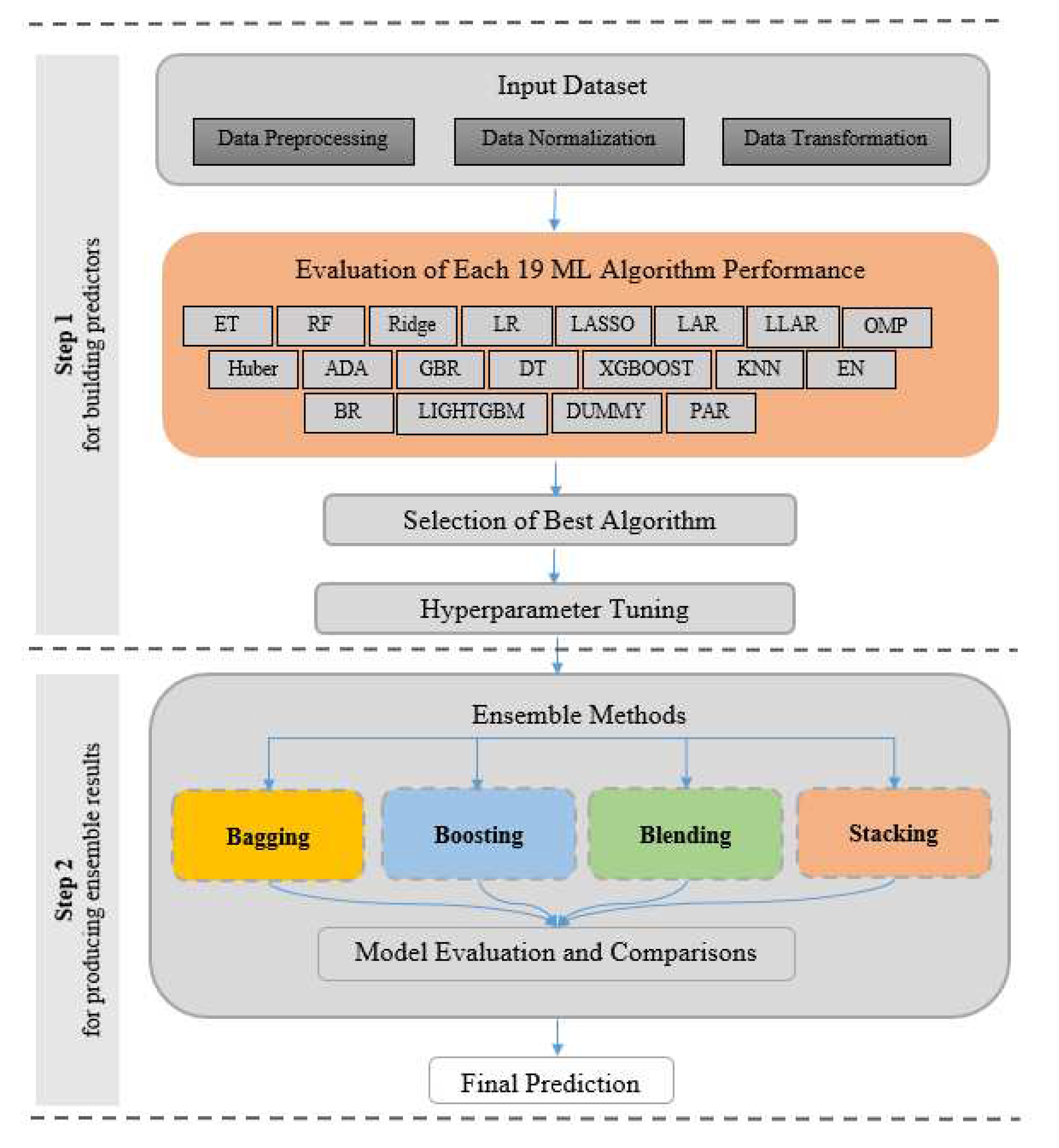
Figure 2.
Correlation matrix of all variables including the target variable.
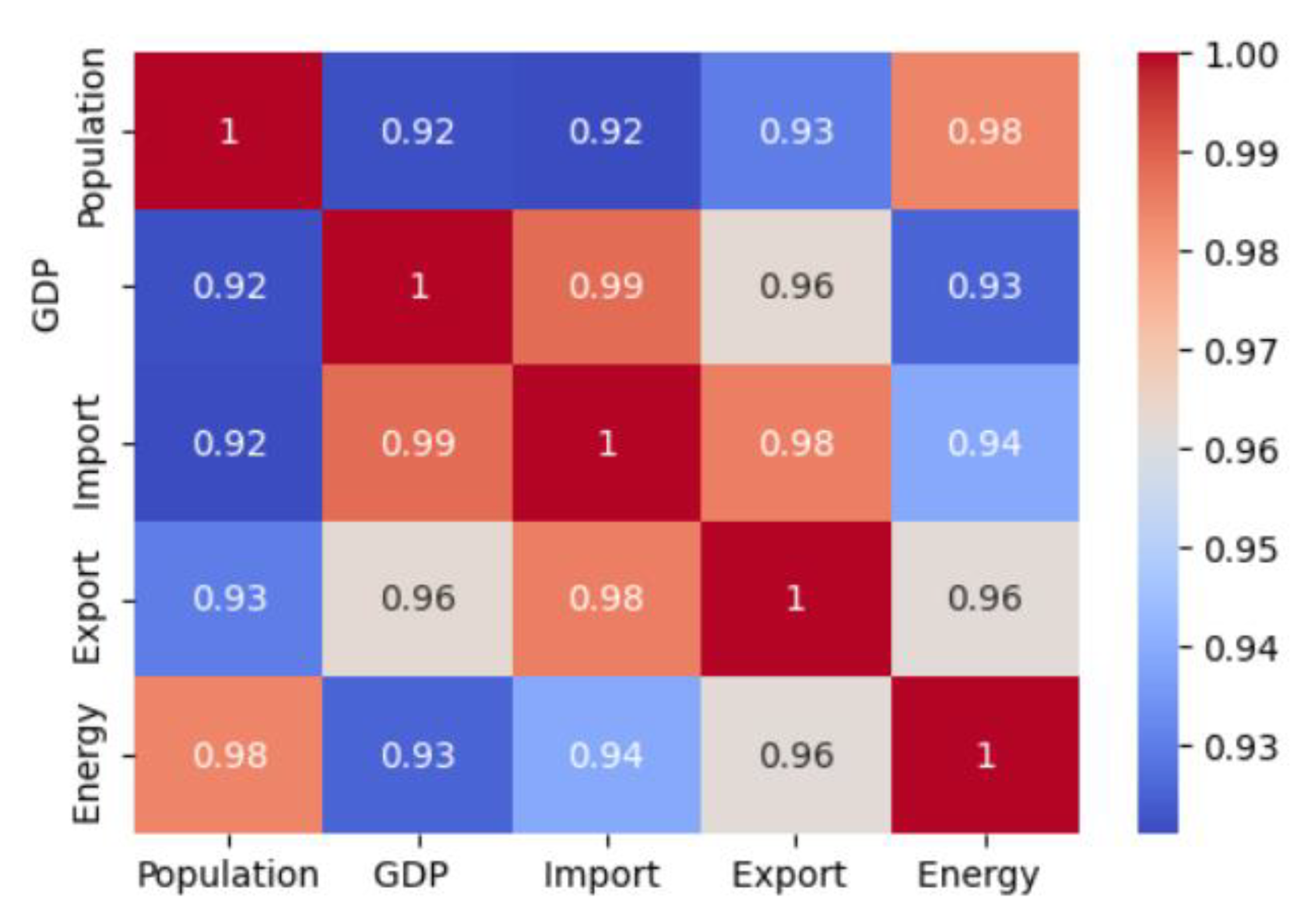
Table 1.
A summary of literature works on Türkiye's energy demand.
| Author(s) | Year | Method used | Dataset | Input Parameters | Forecasting for |
|---|---|---|---|---|---|
| Aslan [48] | 2023 | Archimedes Optimization Algorithm | 1979-2005 1979-2011 | GDP, Population, Import, Export |
Energy |
| Korkmaz [49] | 2022 | Bezier Search Differential Evolution Black Widow Optimization (BWO) |
2000-2017 | Passenger-km, Freight-km, Carbon dioxide emissions, GDP, Infrastructure Investment |
Transportation Energy |
| Aslan and Beşkirli [50] | 2022 | Improved Arithmetic Optimization Algorithm | 1979-2011 | GDP, Population, Import, Export |
Energy |
| Ağbulut [51] | 2022 | Deep Learning (DL) Support Vector Machine (SVM) Artificial Neural Network (ANN) |
1970-2016 | GDP, Population, Vehicle-km, Year |
Transportation Energy |
| Özdemir et al. [52] | 2022 | Modified Artificial Bee Colony Algorithm | 1979-2005 | GDP, Population Import, Export |
Energy |
| Özkış [53] | 2020 | Vortex Search Algorithm (VS) | 1979-20051979-2011 | GDP, Population, Import, Export |
Energy |
| Tefek et. al. [54] | 2019 | Hybrid gravitational search, teaching, learning-based optimization method | 1980-2014 | Population, GDP, Installed power, Gross Generation, Net Consumption |
Energy |
| Beskirli et al. [55] | 2018 | Artificial Algae Algorithm (AAA) | 1979-2005 | GDP, Population, Import, Export |
Energy |
| Cayir Ervural and Ervural [56] | 2018 | Grey Prediction Model Based on GA Grey Prediction Model Based on PSO |
1996-2016 | Previous Annual Electricity Consumption Data | Energy |
| Koç et al. [57] | 2018 | Gravity Search Algorithm (GSA), Invasive Weed Optimization Algorithm (IWO) | 1979-2011 | GDP, Population, Import, Export |
Energy |
| Öztürk and Öztürk [58] | 2018 | ARIMA | 1970-2015 | Previous Energy Consumption Data | Energy |
| Beskirli et al. [59] | 2017 | Differential Evolution Algorithm (DE) | 1979-2011 | GDP, Population, Import, Export |
Energy |
| Daş [60] | 2017 | Neural Network Based on Particle Swarm Optimization | 1979-2005 | GDP, Population, Import, Export |
Energy |
| Kankal and Uzlu [61] | 2017 | ANN | 1980-2012 | GDP, Population, Import, Export |
Electricity Energy |
| Uguz et al. [62] | 2015 | Artificial Bee Colony with Variable Search Strategies (ABCVSS) | 1979-2005 | GDP, Population, Import, Export |
Energy |
| Tutun et al. [63] | 2015 | Regression and ANN | 1975-2010 | Imports, Exports, Gross generation, Transmitted energy |
Electricity Energy consumption |
| Kıran et al. [64] | 2012 | Hybrid Meta-Heuristic (Particle Swarm Optimization, Ant Colony Optimization) | 1979-2005 | GDP, Population, Import, Export |
Energy |
| Kankal et al. [65] | 2011 | Regression Analysis/ ANN | 1980-2007 | GDP, Population, İmport, Export, Employment |
Energy |
| Ediger and Akar [66] | 2007 | Autoregressive Integrated Moving Average (ARIMA) and seasonal ARIMA (SARIMA) | 1950-2005 | Energy | |
| Ünler [17] | 2008 | Particle Swarm Optimization | 1979-2005 | GDP, Population, Import, Export |
Energy |
| Toksarı [67] | 2007 | Ant Colony Optimization | 1970-2005 | Population, GDP, Import, Export |
Energy |
| Sözen et al. [68] | 2005 | ANN | 1975-2003 | Population, Gross Generation, Installed Capacity, Import, Export |
Energy |
| Canyurt et al. [69] | 2004 | Genetic Algorithm | 1970-2001 | GDP, Population Import, Export |
Energy |
| Ceylan and Öztürk [70] | 2004 | Genetic Algorithm | 1970-2001 | GDP, Population, Import, Export |
Energy |
| Ceylan et al. [71] | 2004 | Genetic Algorithm | 1990-2001 | GDP, Population, Import, Export |
Energy and exergy production and consumption |
Table 2.
Input parameter use rationales.
| Variable | The influencing factors for using this variable |
|---|---|
| GDP | There exists a strong correlation between GDP and energy consumption, as the level of economic activity directly impacts the demand for energy. When the GDP of a country increases, it generally indicates a growth in industrial and commercial activities, leading to higher energy consumption. Considering the substantial impact of GDP on energy demand, GDP is often chosen as an independent variable in studies analyzing energy consumption patterns. |
| Population | Population growth directly affects the demand for energy in a country or region. As the population increases, there is a greater need for energy to meet the demands of the growing population, including residential, commercial, industrial, and transportation sectors. Understanding and considering population values as an independent variable is crucial for analyzing and planning energy resources. |
| Import | The relationship between imports and energy consumption is significant, as the availability and reliance on imported energy resources can directly impact a country's energy demand. The import values of energy resources are choosen as independent variables in this study due to their influence on the overall energy consumption patterns. |
| Export | The relationship between exports and energy consumption is an important aspect of understanding a country's energy demand. The export values of energy resources are choosen as independent variables in this study due to their potential impact on a country's overall energy consumption patterns. |
Table 3.
Observed historical data related to the energy demand in Türkiye.
| Years | Population (106) | GDP ($ 109) |
Import ($ 109) |
Export ($ 109) |
Energy (Mtoe) |
|---|---|---|---|---|---|
| 1979 | 43.19 | 82.00 | 5.07 | 2.26 | 26.37 |
| 1980 | 44.09 | 68.82 | 7.91 | 2.91 | 27.51 |
| 1981 | 44.98 | 71.04 | 8.93 | 4.70 | 27.60 |
| 1982 | 45.95 | 64.55 | 8.84 | 5.75 | 29.59 |
| 1983 | 47.03 | 61.68 | 9.24 | 5.73 | 30.25 |
| 1984 | 48.11 | 59.99 | 10.76 | 7.13 | 31.75 |
| 1985 | 49.18 | 67.23 | 11.34 | 7.96 | 32.73 |
| 1986 | 50.22 | 75.73 | 11.10 | 7.46 | 34.59 |
| 1987 | 51.25 | 87.17 | 14.16 | 10.20 | 38.70 |
| 1988 | 52.28 | 90.85 | 14.34 | 11.66 | 39.73 |
| 1989 | 53.31 | 107.14 | 15.80 | 11.62 | 40.40 |
| 1990 | 54.32 | 150.68 | 22.30 | 12.96 | 42.24 |
| 1991 | 55.32 | 150.03 | 21.05 | 13.59 | 43.09 |
| 1992 | 56.30 | 158.46 | 22.87 | 14.71 | 44.70 |
| 1993 | 57.30 | 180.17 | 29.43 | 15.35 | 48.26 |
| 1994 | 58.31 | 130.69 | 23.27 | 18.11 | 45.77 |
| 1995 | 59.31 | 169.49 | 35.71 | 21.64 | 50.53 |
| 1996 | 60.29 | 181.48 | 43.63 | 23.22 | 54.85 |
| 1997 | 61.28 | 189.83 | 48.56 | 26.26 | 57.99 |
| 1998 | 62.24 | 275.97 | 45.92 | 26.97 | 57.12 |
| 1999 | 63.19 | 256.39 | 40.67 | 26.59 | 55.22 |
| 2000 | 64.11 | 274.30 | 54.50 | 27.77 | 61.60 |
| 2001 | 65.07 | 201.75 | 41.40 | 31.33 | 55.60 |
| 2002 | 65.99 | 240.25 | 51.55 | 36.06 | 59.49 |
| 2003 | 66.87 | 314.59 | 69.34 | 47.25 | 64.59 |
| 2004 | 67.79 | 408.88 | 97.54 | 63.17 | 68.24 |
| 2005 | 68.70 | 506.31 | 116.77 | 73.48 | 70.33 |
| 2006 | 69.60 | 557.06 | 139.58 | 85.53 | 74.82 |
| 2007 | 70.47 | 681.34 | 170.06 | 107.27 | 79.79 |
| 2008 | 71.32 | 770.46 | 201.96 | 132.03 | 77.76 |
| 2009 | 72.23 | 649.27 | 140.93 | 102.14 | 78.36 |
| 2010 | 73.20 | 776.99 | 185.54 | 113.88 | 79.84 |
| 2011 | 74.17 | 838.76 | 240.84 | 134.91 | 84.91 |
| 2012 | 75.28 | 880.56 | 236.55 | 152.46 | 88.84 |
| 2013 | 76.58 | 957.78 | 260.82 | 161.48 | 88.07 |
| 2014 | 78.11 | 938.95 | 251.14 | 166.50 | 89.25 |
| 2015 | 79.65 | 864.32 | 213.62 | 150.98 | 99.47 |
| 2016 | 81.02 | 869.69 | 202.19 | 149.25 | 104.57 |
| 2017 | 82.09 | 859.00 | 238.72 | 164.50 | 111.65 |
| 2018 | 82.81 | 778.47 | 231.15 | 177.17 | 109.44 |
| 2019 | 83.48 | 759.94 | 210.35 | 180.83 | 110.65 |
| 2020 | 84.14 | 720.30 | 219.52 | 169.64 | 113.70 |
| 2021 | 84.78 | 819.04 | 271.42 | 225.29 | 123.86 |
Table 4.
The combinations of features.
| Model | Input |
| M1 | GDP, Population |
| M2 | GDP, Import |
| M3 | GDP, Export |
| M4 | Population, Import |
| M5 | Population, Export |
| M6 | Import, Export |
| M7 | GDP, Population, Import |
| M8 | GDP, Population, Export |
| M9 | Population, Import, Export |
| M10 | GDP, Import, Export |
| M11 | *GDP, Population, Import, Export |
* All features.
Table 5.
Top three results of ML algorithms based on the train set using models’ combinations.
| Models | ML Algorithm | MAE | MSE | RMSE | R2 | MAPE |
|---|---|---|---|---|---|---|
| M1 | Extra Trees Regressor | 2743.27 | 14435527.00 | 3622.18 | 0.9751 | 0.0546 |
| Huber Regressor | 3419.46 | 20734897.00 | 4395.82 | 0.9642 | 0.0749 | |
| Extreme Gradient Boosting | 3725.91 | 22807495.50 | 4551.60 | 0.9625 | 0.0655 | |
| M2 | K Neighbors Regressor | 6881.86 | 84149616.80 | 8596.44 | 0.8710 | 0.1104 |
| Random Forest Regressor | 6809.08 | 114145888.80 | 9963.98 | 0.8252 | 0.1167 | |
| Extra Trees Regressor | 6452.43 | 123658755.00 | 9929.56 | 0.8117 | 0.1178 | |
| M3 | Extra Trees Regressor | 3977.99 | 44054367.30 | 5730.78 | 0.9299 | 0.0695 |
| Random Forest Regressor | 4631.80 | 55354193.10 | 6583.28 | 0.9162 | 0.0797 | |
| Gradient Boosting Regressor | 5351.58 | 64199913.90 | 7220.71 | 0.9031 | 0.0901 | |
| M4 | Extra Trees Regressor | 3042.48 | 17937995.55 | 3844.90 | 0.9733 | 0.0591 |
| Random Forest Regressor | 3666.07 | 22957290.18 | 4448.29 | 0.9716 | 0.0685 | |
| Gradient Boosting Regressor | 4156.41 | 26308872.75 | 4930.11 | 0.9652 | 0.0742 | |
| M5 | Huber Regressor | 3864.21 | 36775418.87 | 5527.85 | 0.9541 | 0.0601 |
| Lasso Regression | 4003.55 | 36200997.00 | 5456.62 | 0.9530 | 0.0678 | |
| Least Angle Regression | 4003.72 | 36196280.60 | 5456.35 | 0.9530 | 0.0678 | |
| M6 | K Neighbors Regressor | 5707.22 | 80792845.60 | 7992.88 | 0.8962 | 0.1035 |
| Random Forest Regressor | 5455.21 | 77021388.80 | 8193.73 | 0.8644 | 0.0930 | |
| Extra Trees Regressor | 5511.29 | 82472925.80 | 8300.80 | 0.8540 | 0.0950 | |
| M7 | Extra Trees Regressor | 2308.94 | 12339053.90 | 3277.79 | 0.9754 | 0.0488 |
| Random Forest Regressor | 2972.75 | 17408515.60 | 3854.32 | 0.9608 | 0.0576 | |
| AdaBoost Regressor | 3400.27 | 18546026.70 | 4014.45 | 0.9538 | 0.0640 | |
| M8 | Extra Trees Regressor | 3189.81 | 17110325.38 | 3874.79 | 0.9716 | 0.0537 |
| AdaBoost Regressor | 4293.89 | 29715232.81 | 5282.08 | 0.9475 | 0.0728 | |
| Random Forest Regressor | 4287.09 | 35730037.10 | 5185.02 | 0.9460 | 0.0700 | |
| M9 | Extra Trees Regressor | 3018.13 | 30503239.40 | 4394.13 | 0.9477 | 0.0407 |
| Random Forest Regressor | 3583.32 | 45575422.90 | 5273.91 | 0.9304 | 0.0473 | |
| AdaBoost Regressor | 4069.59 | 37580683.81 | 5358.08 | 0.9285 | 0.0609 | |
| M10 | K Neighbors Regressor | 5670.51 | 74121506.00 | 7652.91 | 0.9017 | 0.1003 |
| Random Forest Regressor | 5372.22 | 75187291.90 | 7930.92 | 0.8896 | 0.0942 | |
| Ridge Regression | 7009.35 | 69191604.80 | 8277.45 | 0.8621 | 0.1643 | |
| M11 | Extra Trees Regressor | 2296.86 | 8756864.57 | 2932.96 | 0.9788 | 0.0464 |
| Random Forest Regressor | 3186.05 | 14777499.11 | 3817.37 | 0.9684 | 0.0658 | |
| Ridge Regression | 3676.12 | 21641675.00 | 4466.13 | 0.9655 | 0.0736 |
Table 8.
Performance of the ensemble models in both the training and test dataset.
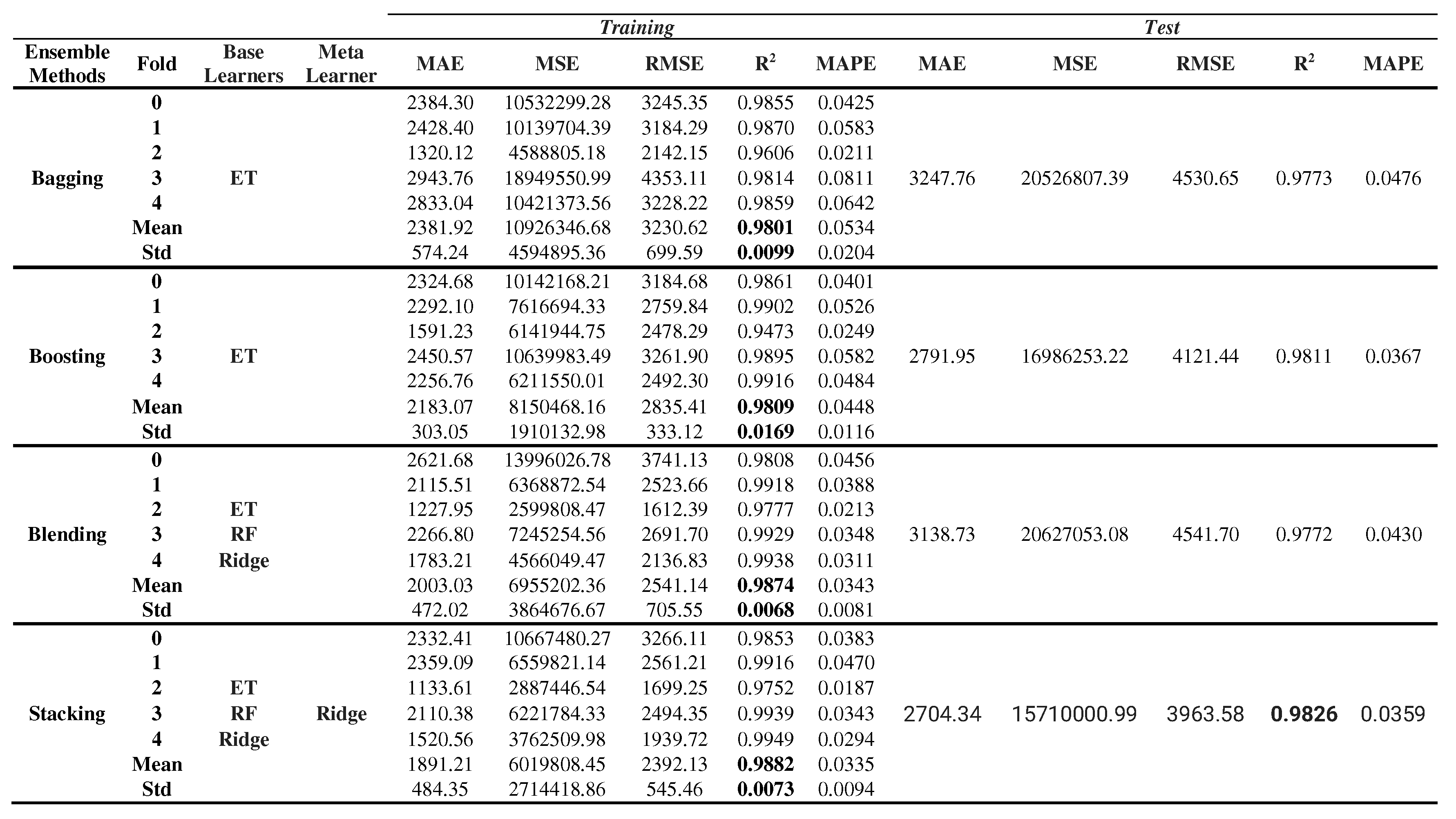
Table 9.
Comparison of the actual values 'Energy' and predicted values using the proposed stacking ensemble model.
Table 9.
Comparison of the actual values 'Energy' and predicted values using the proposed stacking ensemble model.
| Sample Size | Population | GDP | Import | Export | Energy | Prediction |
|---|---|---|---|---|---|---|
| 1 | 65988664 | 2.40E+11 | 51553796 | 36059088 | 59486 | 62736.99 |
| 2 | 70468872 | 6.81E+11 | 170062720 | 107271752 | 79785 | 76948.98 |
| 3 | 44089068 | 6.88E+10 | 7909364 | 2910122 | 27507.96 | 26962.77 |
| 4 | 76576120 | 9.58E+11 | 260822800 | 161480912 | 88074.43 | 91513.96 |
| 5 | 78112072 | 9.39E+11 | 251142432 | 166504864 | 89248.78 | 96054.71 |
| 6 | 47026424 | 6.17E+10 | 9235002 | 5727834 | 30249.94 | 28972.36 |
| 7 | 52275888 | 9.09E+10 | 14335398 | 11662024 | 39733.94 | 38689.99 |
| 8 | 84775408 | 8.19E+11 | 271424480 | 225291392 | 123859.48 | 113726.34 |
| 9 | 48106764 | 6.00E+10 | 10757032 | 7133604 | 31747.45 | 30416.86 |
| 10 | 73195344 | 7.77E+11 | 185544336 | 113883216 | 79840.07 | 81925.22 |
| 11 | 53305232 | 1.07E+11 | 15792143 | 11624692 | 40395.43 | 40529.37 |
Disclaimer/Publisher’s Note: The statements, opinions and data contained in all publications are solely those of the individual author(s) and contributor(s) and not of MDPI and/or the editor(s). MDPI and/or the editor(s) disclaim responsibility for any injury to people or property resulting from any ideas, methods, instructions or products referred to in the content. |
© 2023 by the authors. Licensee MDPI, Basel, Switzerland. This article is an open access article distributed under the terms and conditions of the Creative Commons Attribution (CC BY) license (http://creativecommons.org/licenses/by/4.0/).
Copyright: This open access article is published under a Creative Commons CC BY 4.0 license, which permit the free download, distribution, and reuse, provided that the author and preprint are cited in any reuse.


