1. Introduction
Nowadays generative artificial intelligence is one of the top themes of computer engineering research. The emergence of transformers [
1,
2] as a key tool for generating content has opened a world of new applications where automated systems are able to create productions that, until now, were exclusive of human authorship. Transformers were first used for automated translation systems, where a first processing stage (the encoder) transforms the input text into a numerical representation of text meaning; then a second stage (the decoder) converts (like an inverse transform) those intermediate data into text in another language [
3].
Besides neural machine translators, other impressive applications have arisen. Famous chatGPT is a conversational engine created with a decoder transformer [
4,
5]. Using also transformers, models for translating regular text into images have also been developed. Most known and documented examples of these last ones are DALL E [
6,
7] and Stable Diffusion [
8]. But other examples have quickly been released like: OpenArt [
9], ImagineArt [
10], Adobe Firefly [
11] and many others.
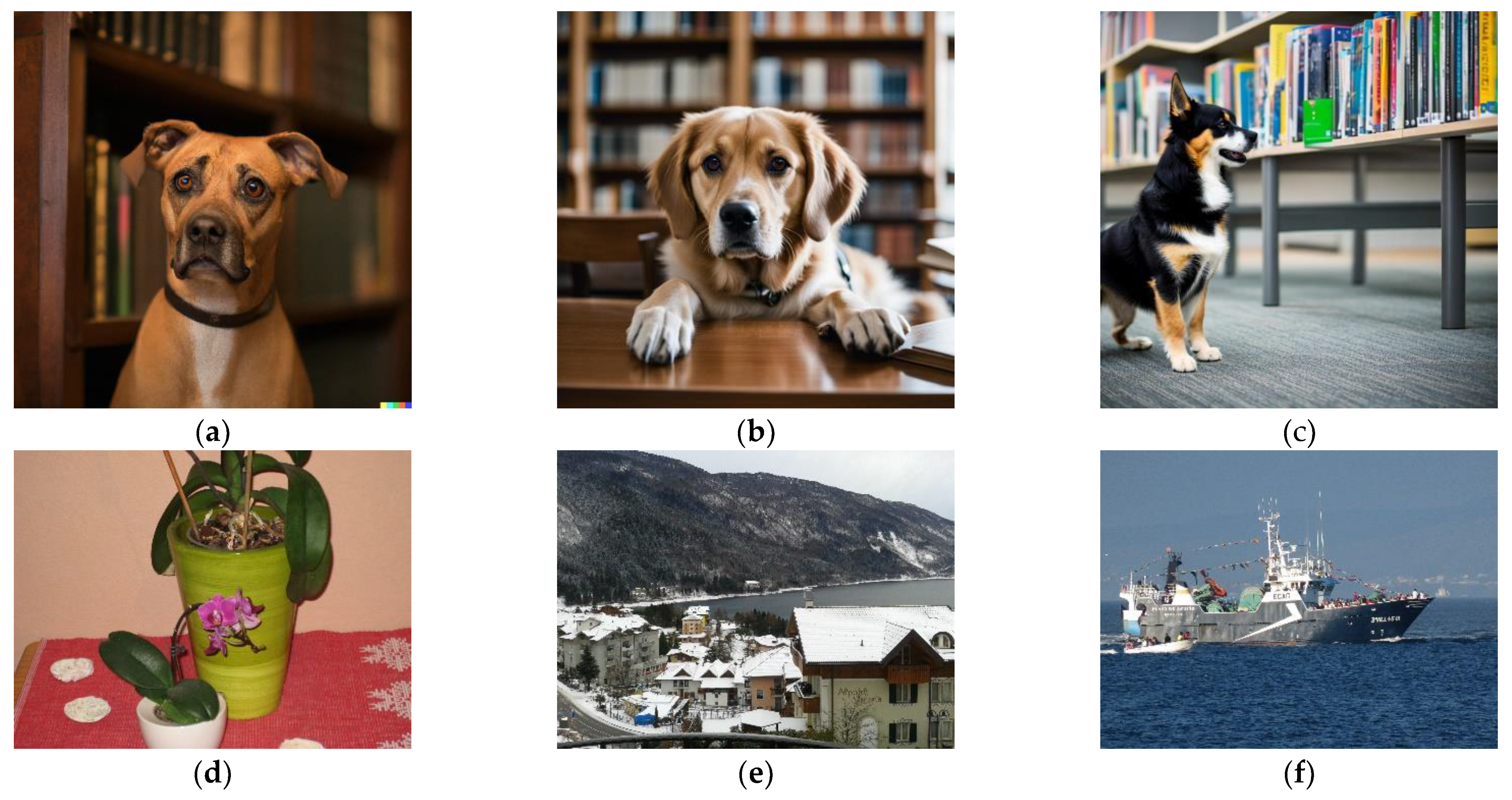
These artificial image generators have reached the point where they may create photo realistic images that can make humans to hesitate if a particular image is really coming from a camera or is an artificial creation. As an example, in
Figure 1, three IA created images are presented. They have been created by three different engines: DALL E 2, Stable Diffusion and OpenArt (after testing many applications, these three were found the most appropriate for photorealistic images; other models are good on producing drawings or illustrations, not so much on imitating real photographs). Prompt was the same for the three images: “realistic photo, a portrait of a dog in a library, Sigma 85 mm f/1.4”. Note that details about lens have been added (85 mm focal lens, f/1.4 numeric aperture), this is a common trick used for getting more realistic results. In the same figure, we present also three real photographs that will be processed later. The purpose of this work is making automatically a binary decision between two options: AI-image (fully created AI image) and real image.
Other impressive AI application is Deep Fake [
12,
13]. Deep Fake is able to create photos and videos mixing plausibly information from previous photos and/or videos. For example, creating a video of a person mixing the body from one given individual and the face of another one. The potential danger of this technology being used for fraud or other illegal purposes (defamation, pornography…) has sparked much research on the field of detecting Deep Fake image creation [
14]. For example, in [
15], Rössler et al start by creating a large dataset of fake videos. In [
16], authors exploit what it is, perhaps, the most intuitive method: finding image artifacts that can reveal synthetic content. In [
17] a system called “FakeCatcher” is described; this system works relying on biological signals, like the small periodic color variations present in a real face video by cause of the person’s heart rate. A very recent paper by Becattini et al [
18] presents a Deep Fake detector based on Head Pose Estimation (HPE). In [
19], Bappy et al present a general image forgery detector based on recursive neural networks (LSTM). Almost all publications in this field claim that direct use of neural networks does not produce good results in these kinds of applications. In [
20], authors use detection of “convolutional traces”, basing themselves on the fact that AI generated images have passed several convolution stages.
The work described in this paper is similar to Deep Fake detection but with a different purpose. The target is to automatically detect AI generated photo realistic images, id Est: distinguishing whole AI images from real photographs. AI images are not supposed to represent or try to represent any particular real object, place or individual. This can be interesting for classifying images in photography websites and/or in social networks. Note that, in this case, the system is dealing with all kind of images: human faces, animals, still nature, landscapes… For this reason, it is not possible to rely on some of the “face related” characteristics. Relying on artifacts may work for some images but not for all. Artifacts are common in artificial images within some detailed parts (the fingers of a person’s hand, pedals of a bike), but in many images there are no visible errors. What’s more, there are some evident errors, like persons with three hands or even with two heads, which are evident for human view but not so easy to automate in an autonomous recognition system for any type of image.
For this particular application, there are much less references in the literature. In a recent preprint [
21], authors propose a method for AI images detection using a complex feature extraction based on two parallel deep learning processes. Results are similar to the ones presented in this paper, but they are using a more complex method and their tests have been conducted on images of smaller resolution (maximum 256x256). In [
22], authors construct a huge dataset and they discover that systems trained on one generation model are pretty good on images from that model, but not so much on others. In this work, several models are used to create the dataset and even other different modelsa re tried for finals tests (see discussion section). According to [
23], features extracted for recognition are crucial in this problem when trying to work with different generation models. They point out that statistics of overexposed pixels can be a good election, that seems to reinforce the election of PRNU. Other recommendation is using color related features; ELA pattern used in this paper is strongly color related with color as JPEG error is greater on color components. Other references [
24,
25,
26] focus on CG (Computer Generated) images, which is another type of problem as they are dealing with images that were created with intensive human intervention.
For a similar need, Google has recently announced a new tool, called SynthID [
27] which adds an invisible watermark to AI generated images so that they can be identified. Note that this will indentifyAI images only if creation engine watermarks them.
Because of the need of classifying whole images with no assumption about image content, the system has been designed based on methods from other image forensics applications. The main idea is extracting some relevant information from images before applying a convolutional neural network. Convolutional Neural Networks CCN’s are very useful in distinguishing between classes that are visually different for humans like digit classification [
28,
29], distinguishing objects relevant for taking driving decisions in real traffic and many other similar applications [
30]. Nevertheless, in this case, classes are not visually different and that suggests that direct application of CNN’s could not be very useful (besides the experience from the Deep Fake case). For this reason, pixel wise feature extraction has been used. This means using processing stages that convert images into other images with the same size (it converts each pixel to a new pixel) but containing a reduced amount of information that should be relevant to the particular problem of distinguishing AI images.
Methods used for this issue are, up to date, two. First one is Photo Response Non-Uniformity (PRNU). PRNU is in fact a kind of noise used for source camera identification (distinguishing the camera that has taken a given image) [
31]. The origin of PRNU is the slightly different sensitivity of individual pixels in a real image sensor. This effect is due to manufacturing imperfections and it is unavoidable. AI images should have no PRNU at all. Nevertheless PRNU computation methods always yield some nonzero result. PRNU has been extensively studied, including its limitations [
32,
33]. CNN is trained to infer special characteristics of AI images with false PRNU patterns. There exist applications designed for erasing or even forging PRNU patterns (embedding on an image the pattern of a given camera) [
34]. So this is a method that can reveal images created by “not very expert” or “not very malicious” users.
The second feature extraction method used is Error Level Analysis (ELA). ELA is a special image (or pattern) that detects irregular errors in JPEG coded images. ELA has been successfully used to detect editions in images (thus to authenticate scanned or photographed images) [
35,
36]. ELA has also been applied for forged face detection [
37]. Basically, ELA detects non uniformity in quantization errors due to JPEG compression. Applied to an AI generated image, ELA normally yields a strange result as if all pixels of the image would have been modified by edition. This could be due to the special nature of AI images coming from training with many JPEG coded photographs. So, ELA pattern is also a good choice for the application that this paper is addressing. It would seem that this method also has a limitation: all images, either coming from a real camera or from an AI engine, must be obtained in JPEG format. It would not be a great drawback as JPEG is the most frequent photography format. Nevertheless, as seen in the remainder of this paper, ELA has been successfully tested on AI images obtained in PNG format.
Another possible feature extraction for this problem is Local Binary Pattern (LBP) [
36]. LBP is based on differences between adjacent pixels. An eight-bit word is assigned to each pixel with a binary ‘1’ for greater surrounding pixels and a ‘0’ in other case. This technique has successfully been used for fake faces detection [
39]. LBP is also used to detect fake face presentation to biometric systems with video replays. Patel [
40] explored this approach detecting moiré patterns with LBP features.
The remainder of the paper is organized as follows: in
Section 2, methods and processing are described as well as the image dataset used for training and testing; in
Section 3, results are summarized. In the Discussion section, the main results of this work are highlighted.
2. Materials and Methods
2.1. The Dataset
The dataset used in this work for training and testing is composed of a collection of images divided in two groups (or classes): AI generated and real camera photographs. First, AI generated images were created by authors using three different engines: DALL E, Stable Diffusion and OpenArt. These images were visually checked to discard those that were not photo-realistic. Second, real photos were selected randomly from image databases. There are images from Dresden Image Database [
41], also from VISION dataset [
42] and also from authors’ provided images that were already used in previous studies [
33,
43]. There are real photos from the following cameras: Canon Ixus 70 (two instances), Casio Ex Z150 (two instances), Canon PhotoSmart SX720, Canon EOS 1100D, Kodak M1063 (two instances) and Sony ILCE 5000. Photos from smartphones are also included: Huawei P20, Huawei P9, Samsung Galaxy S3 Mini, Apple Iphone 4s, Apple Iphone 5c, Apple Iphone 6 and LG D290.
Initially, the dataset was made up of 459 AI generated images and the same number of real photographs (a total of 918 images). Afterwards, an extended dataset of 1252 was tested. Both datasets are fully balanced (same number of samples on each class). On each test a percentage of dataset samples will be used for training, leaving the remainder for validation.
2.2. PRNU Extraction.
As the name: Photo Response Non-Uniformity, indicates PRNU comes from the different light sensitivity of the different pixels (elementary sensors). This is an unavoidable characteristic due to manufacturing imperfections and it is present on all image sensor chips. PRNU is seen as a multiplicative noise that responds to the following equation [
42]:
Where Imin is the “real” image presented to the camera (the incident light intensity), Iones is a matrix full of ones and Noisecam is the “sensor noise pattern” (PRNU pattern) and Imout is the final image surrendered by the camera. The symbol “.” means matrix point by point (pixel-wise) product and Noiseadd is additive noise from other sources.
PRNU is computed from an image (or from a collection of images coming from the same camera) performing a denoising process on Im
out, and then computing a residual:
Neglecting the additive noise and assuming that Im
in = denoise(Im
out), given a collection of images from the same camera, the PRNU pattern (sometimes called camera fingerprint) can be estimated as:
Note that, in this application, we will always compute PRNU fingerprints with a single image (N=1) both for AI generated and for real images. In this case, F=W/Imin (pixel wise quotient) and it is clear that we will get some result, even for AI images.
Note that “denoising” is a noise reduction filter. For this problem, there are several options documented in the literature: median filter [
44], Wiener filter [
45] and also variations of Wiener filter. In this study, a Matlab [
46] implementation from [
47] is used, this software uses a Wavelet Transform [
48] based Wiener filter.
From each image, a centered square 512x512 region is extracted to work with smaller images and to avoid logos or visible watermarks (that anyway are not present on the dataset images) and PRNU is computed from the sub-image. Note that problem is classifying the whole image, not detecting a “modified” part. Minimum image size for this version is then: 512x512. System can be tailored easily for smaller sizes but that would require retraining.
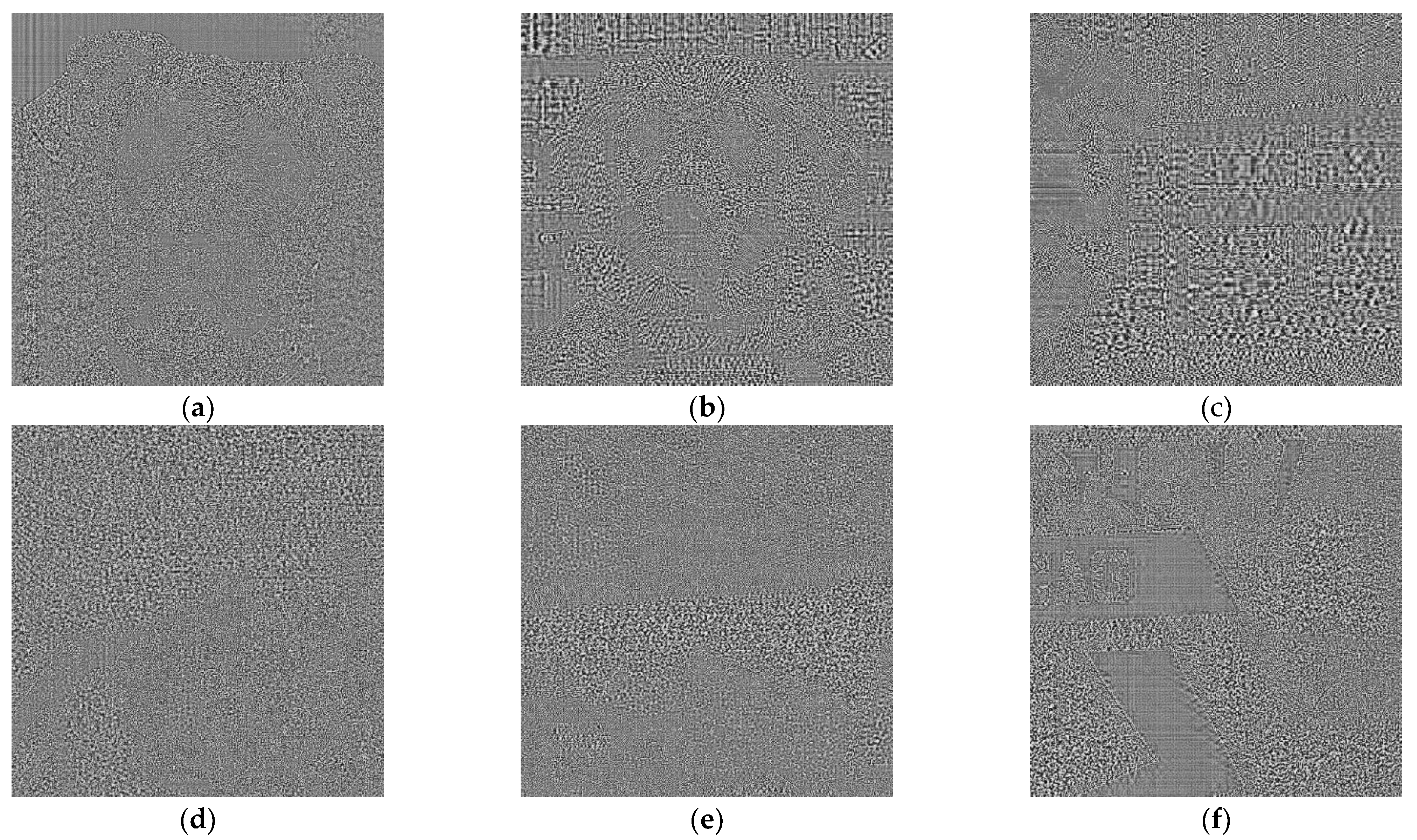
The results of this process are noise like images very difficult to be interpreted visually (see
Figure 2 where PRNU patterns are shown for images of
Figure 1, histogram equalization has been applied to enhance a bit these images). Note that equation 2 can be seen as a high pass filter and so, the results contain part of image contours (a normal phenomenon when computing the pattern from a single image). There seems to be no significant visible difference between AI images: (
a), (
b) and (
c) and real ones: (
d), (
e) and (
f).
2.3. ELA Error Level Analysis.
ELA pattern is computed to detect irregular distributions of quantization noise. This is a tool normally used to detect image editions. An ELA pattern is normally computed coding the whole image with JPEG standard at a known, constant, normally at a high-quality level (a typical value is 95%); then the decoded image from the JPEG bit stream is subtracted from the original image.
If we are facing an edited image, an irregular pattern with different intensities will appear. In
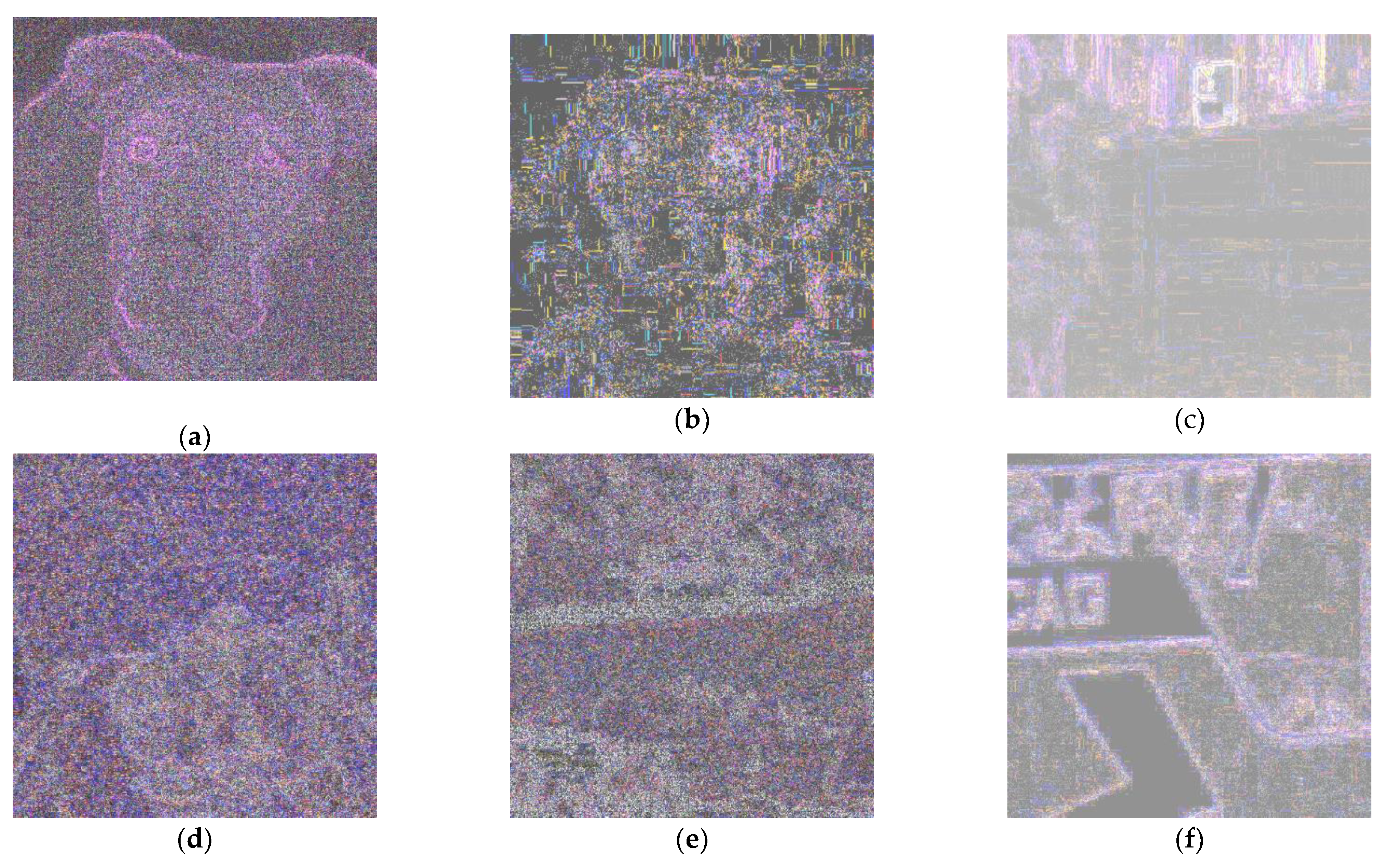
Figure 3, ELA patterns for the same original images (
Figure 1) are shown, Again, histogram equalization has been applied to enhance a bit these images.
Note that, in this case, patterns are color images. For PRNU computation, images are converted to grayscale, prior to all processing. Images are again cropped to the central square sub-image of size 512x512.
Again, a “high pass filtering” effect is evident. Visual differences between AI images AI images: (a), (b) and (c) and real ones: (d), (e) and (f); are again not very remarkable. Perhaps, contours are more evident in the above part but it does not seem conclusive. Nevertheless, neural networks can be able to learn differences that are not perceived by humans.
Figure 3.
(
a), (
b) and (
c), ELA patterns computed for images of
Figure 1. (
d), (
e) and (
f) are examples of ELA patterns for real images used to compute
Figure 2.
Figure 3.
(
a), (
b) and (
c), ELA patterns computed for images of
Figure 1. (
d), (
e) and (
f) are examples of ELA patterns for real images used to compute
Figure 2.
2.4. CNN’s Convolutional Neural Networks.
CNN’s are basically a cascade of convolutional (or linear filtering) stages accompanied by others of non-linear activation, normalization and decimation. These stages extract high level features from low level data (pixels) and so, CNN’s are able to process images directly with no need of feature extraction. The initial image is repeatedly filtered and decimated, creating a set of several small images that are finally processed by a classical perceptron (fully connected) stage to get the final result. This final result is a numerical vector of as many components as classes to be recognized. The Softmax normalization (the most frequently used at final stage of CNN’s) makes that vector components lie in the range 0.0-1.0 and besides, they always add up to 1.0. The maximum component defines which one is the recognized class.
Filter coefficients and perceptron weights are all optimized through the training process. Training algorithm is Stochastic Gradient Descent with Momentum (SGDM) [
49] that is a gradient-type optimization that minimizes mean square error between the obtained and desired output.
In this paper, a previous image to image transformation is done that acts as a pixel-wise feature extraction. This stage tries to search for relevant characteristics for distinguishing classes, removing unimportant information. As reported in the case of Deep Fake detection, direct CNN application is not good for this type of problem.
The dataset is divided randomly, selecting 85% images of each class for training and leaving the rest for validation. Note that the dataset is balanced (it has the same number of samples for each class). A validation stage is performed at each training epoch, adequately controlling the learning process. Each complete epoch (run of all training samples in random order) is divided into n iterations. Each of the iterations is a mini-batch, this is: a set of samples that is processed without updating weights (mini-batch size is DatasetSize/n). Testing values for n, optimum results were obtained for n=3.
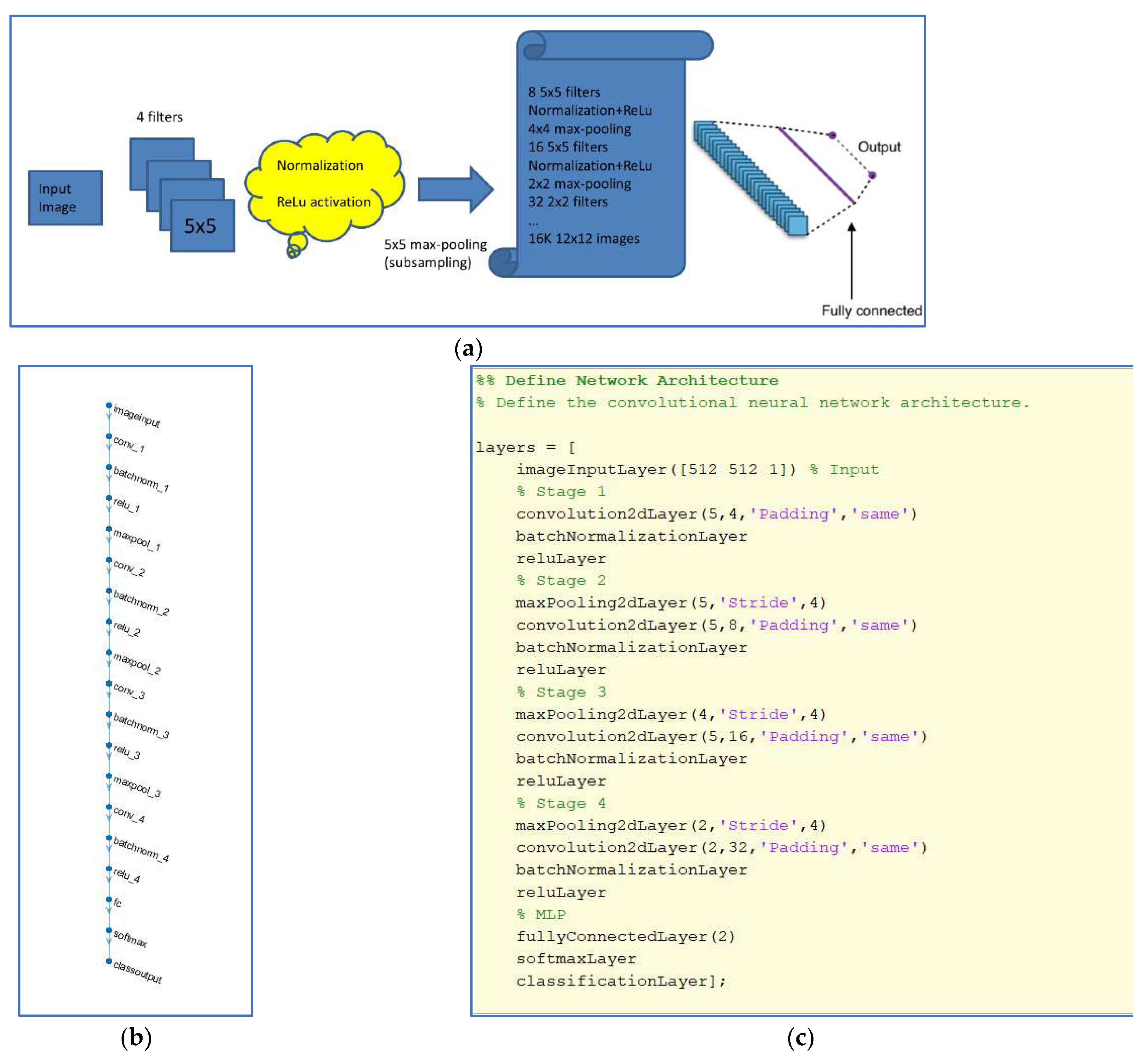
CNN structure: the number of stages and filter configuration at each stage is shown in
Figure 4. And it is the same for the two kinds of pattern extraction techniques tested.
At the end of training, a confusion matrix is computed for the validation set. This means, counting the number of True-Positive (AI images correctly detected), False-Negative (AI images not detected), False-Positive (real photographs detected as AI) and True-Negative (real photographs detected as real). The matrix is arranged in this manner:
From this matrix, several performance measurements can be computed:
Accuracy is simply the success rate. The other three parameters are very easy to interpret and are very typical in classification systems: P (Precision) would be the probability of true detection for true cases; R (recall) would be the probability for effective detection of true cases. F1-score is the harmonic mean of P & R. Obviously, the greater these quantities are, the better performance is achieved.
3. Results
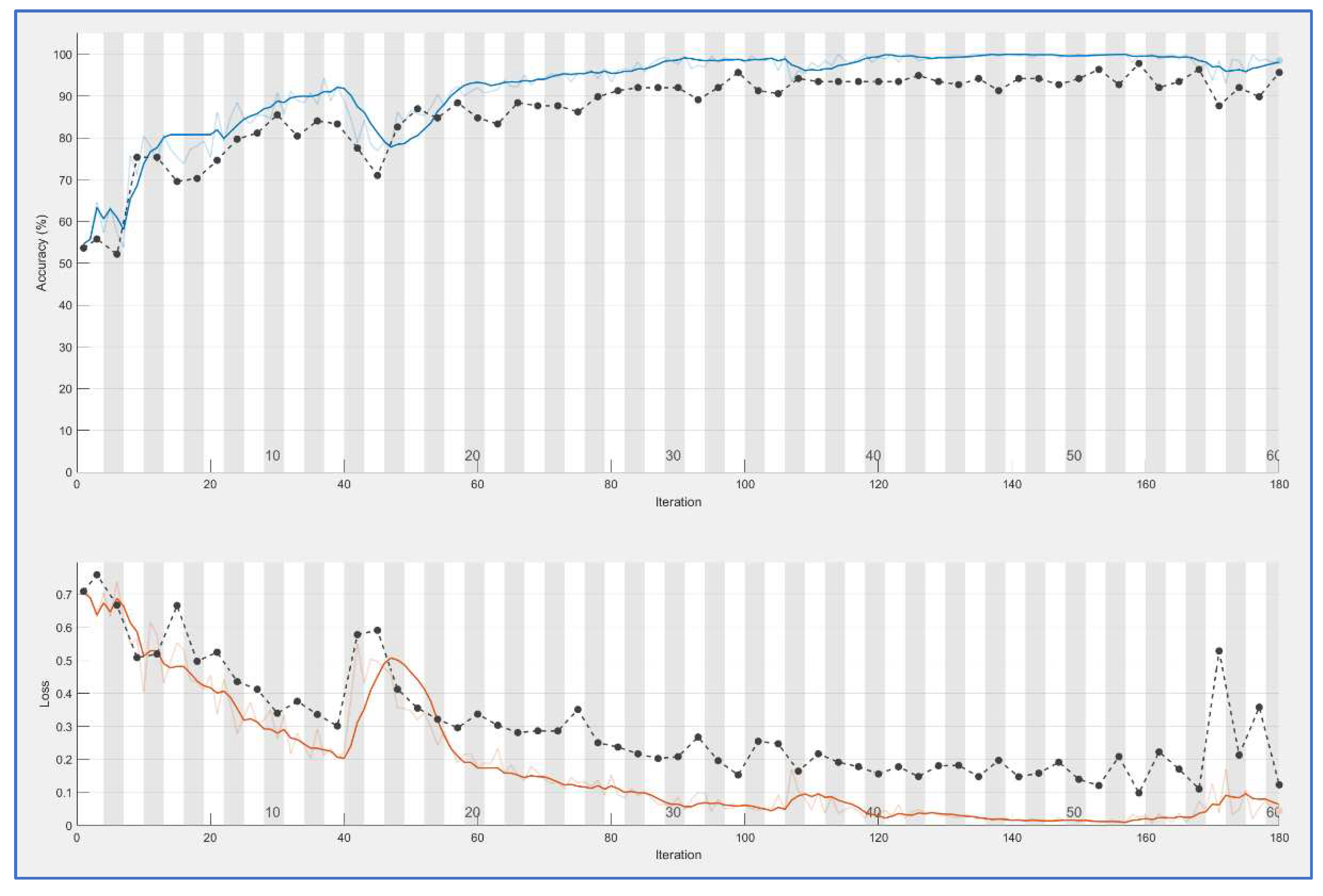
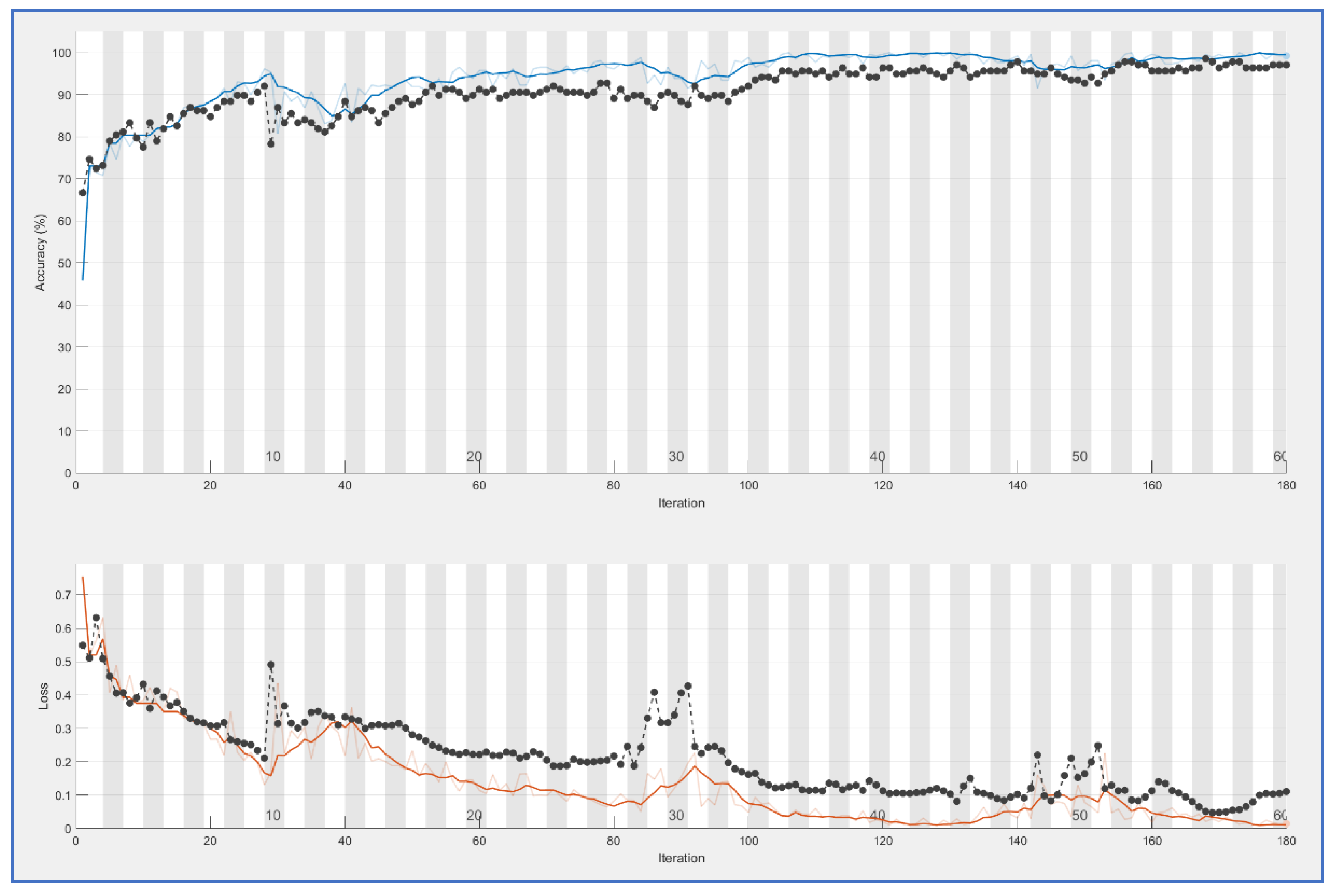
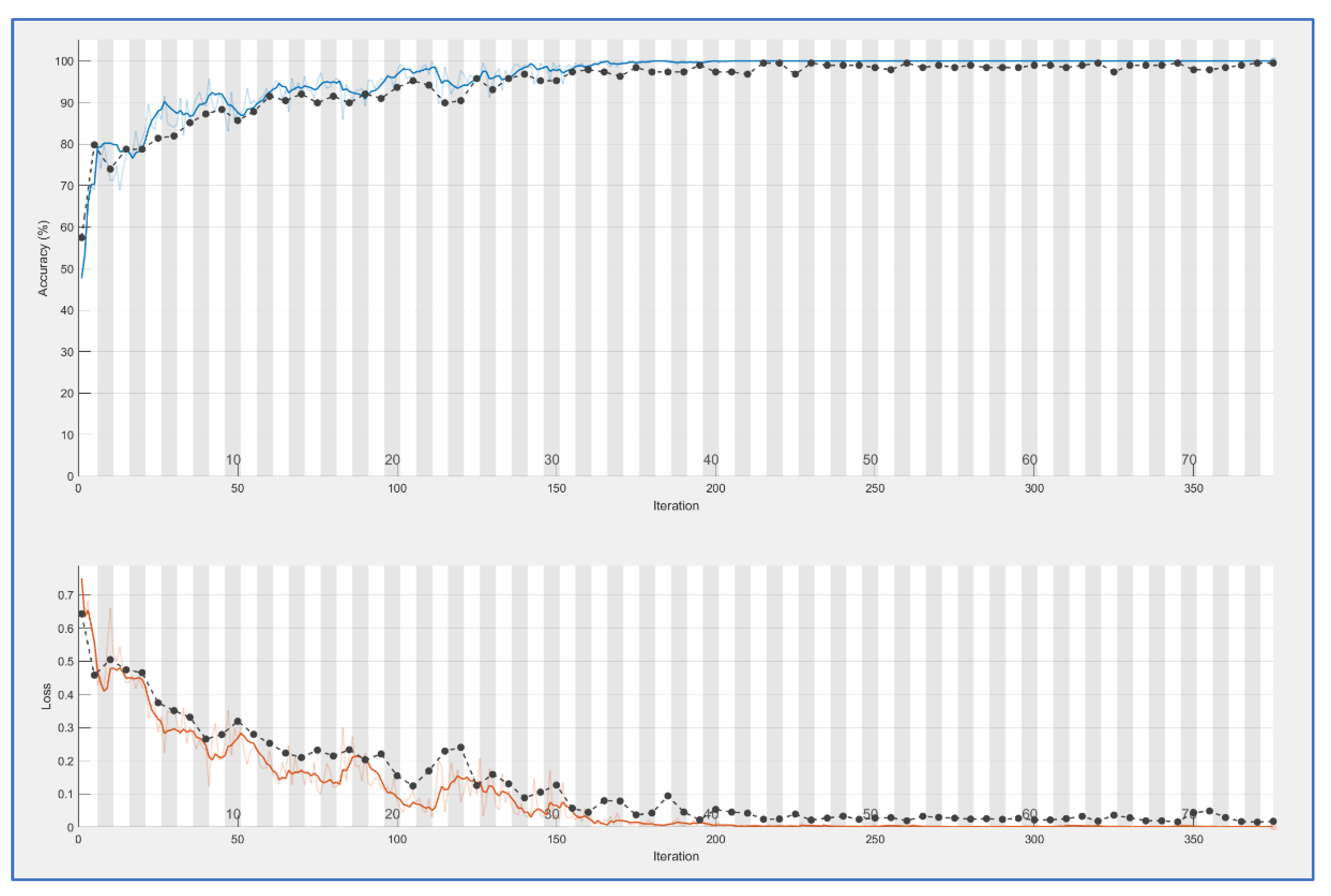
CNN nets were trained and tested for both types of feature extraction. This process produces learning curves displayed in
Figure 5 and
Figure 6. In both cases, a good result is achieved: accuracy is 0.95 for PRNU and 0.98 for ELA. Both trainings have been done with 100 epochs. Training time is bigger for the ELA case (167 minutes versus 109), this is reasonable because ELA images are color ones with three times more information.
Blue curves in both figures are the accuracy values obtained for each iteration (measured on the training samples), black curves are accuracy values for the validation set at each epoch (an epoch is equal to n iterations, with n=3 in this case). The curves below (brown and black) are the mean square error (over training and validation set), this is other method for controlling learning.
In both cases, the fact that black curves follow the evolution of blue/brown curves demonstrates that neural net is generalizing. In the case of overfitting, the blue curve can go high but the black curve would remain low.
Comparing both trainings, ELA offers more stable results.
Figure 5.
CNN training for PRNU patterns.
Figure 5.
CNN training for PRNU patterns.
Figure 6.
CNN training for ELA patterns.
Figure 6.
CNN training for ELA patterns.
These matrices yield the following numbers in the
P,
R and
F1 terms, see
Table 1.
4. Discussion
Last presented results seem to demonstrate again that both methods are good but ELA outperforms PRNU with a slight advantage. These results were obtained with a reduced dataset of 459 images per class. Afterwards, a new test was conducted using an extended version with 626 samples per class. This test was only done with the ELA extraction (the best option). Learning curve is presented in
Figure 7. In this case the
n parameter was set to 5 because with more samples, it is necessary to reduce batch size. Number of epochs is 75 because in previous tests, it was seen that learning for ELA features was already getting stable at that point.
New assessment data for ELA features improve slightly. Confusion matrix becomes:
Accuracy now is 0.99, Precision is 0.99, recall es 1.0 and F1 score is 0.99. To get more insight into these results, we tested a pre-trained classic net. We chose AlexNet [
30]. For this process, image cropping is modified so that we get the required size for input in this CNN: 227x227x3. Three last layers (including the final classification via a fully connected MLP layer) are modified to the new problem of binary classification (two output neurons). Weights for this level are reset to random values. Model is retrained with a very small learning rate at all levels, EXCEPT at the modified ones. Learning parameters are now those recommended for this kind of training: SGDM method [
49], only 4 epochs with a mini-batch size of 10 that results in 106 iterations per ephoc. Again dataset is divided into an 85% part for training and 15% for validation. Confusion matrixes for validation set are the following, where test has been performed with the two feature extraction types: PRNU and ELA.
These matrices yield the following numbers in the
P,
R and
F1 terms, see
Table 2.
Where it can be seen that method is viable but should be refined a bit. Perhaps the pre-trained levels of AlexNet are good for ordinary images but not so well fitted for PRNU/ELA patterns. Up to the point, the preferred method is ELA + specific CNN.
Another test has been carried out presenting to the original system (to the trained CNN’s) a new set of images completely new. Neither used so far in training nor in validation. This new dataset consists of 150 AI generated images and other 150 real photos. Photos have been taken from unused material of VISION database [
42] (they are all smarphone photos). AI images have been created using creation engines different from those of the first dataset: Leonardo.AI [
50] and TensorArt [
51].
Confusion matrixes for this new dataset are now:
These matrices yield the following numbers in the
P,
R and
F1 terms, see
Table 3.
Curiously, in this case, PRNU outperforms ELA. What’s more, seeing that generally real photos are correctly classified (there are no false positives), creating a combined methods is easy. If both methods are executed on the same image, it is enough that one of them classifies it as AI image to consider it an AI image. Running again test with this combination, accuracy goes to 0.97 and F1 score to 0.97. Mean execution time of this combined recognition is 0.43 s per image in the matlab application. The implementation takes advantage of the combination “logical OR” nature: if first method applied yields a AI-image result, it is not necessary to execute the second one.
4.1. Conclusions
In this work, an automated system for detecting AI created images and distinguishing them from real camera photographs has been created.
Direct use of CNN’s over the images seemed not very recommendable, but extracting pattern-like (or pixel-wise) features like PRNU or ELA patterns yields good results. ELA patterns work slightly better although combination of both methods is easy ans improves results.
This issue is relatively new in the world of image forensics. Although there are many publications about detection of image editions including Ai edition and Deep Fake, pure recognition of 100% created AI images with no assumptions about content is less common. The method presented in this paper has been trained with three different creation models and tested with a validation set obtained from the main dataset and also with a new dataset obtained from other different creation models. Examples documented present similar result but on smaller images [
21], good results very dependant on image creation model [
22] (note that when executing a recognition possible creation model is not known). In [
23], authors study feature extraction methods that can be able to recognize AI images coming from different models. The use of ELA patterns is compatible with their findings.
As supplementary results:
A new dataset on AI created images has been created. This set could be augmented and published as a separate result.
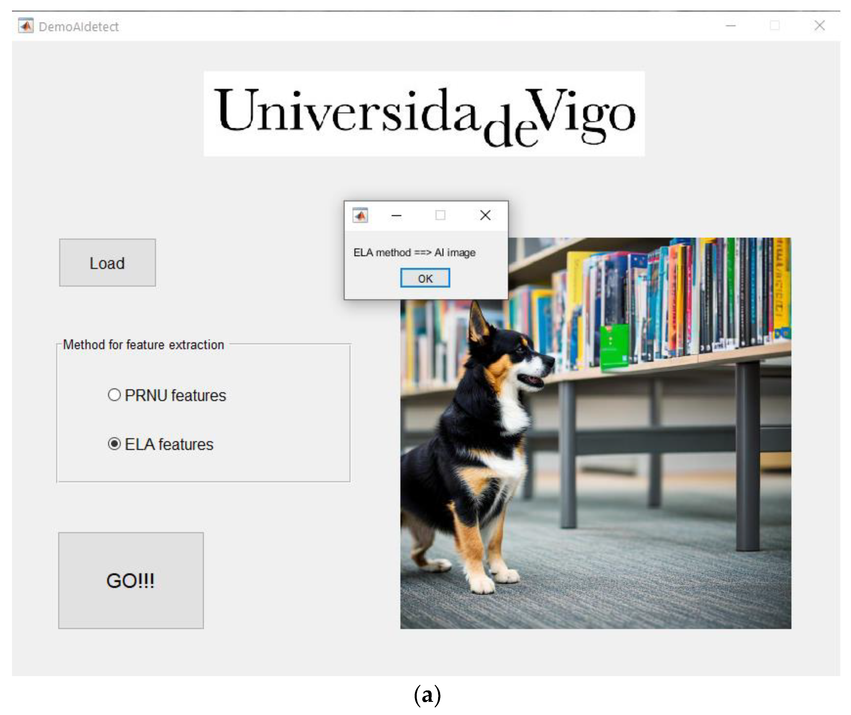
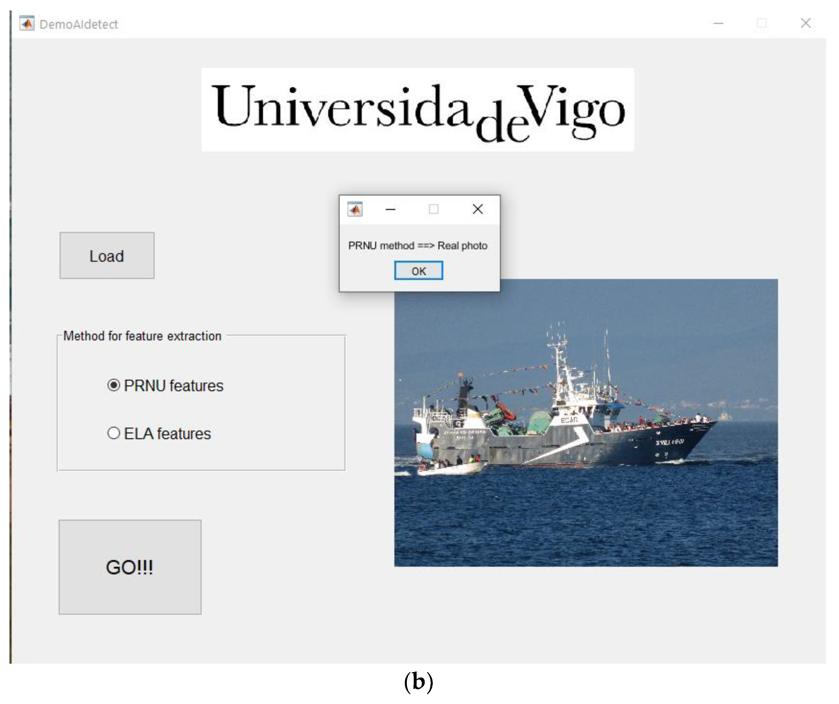
A graphical demo application has been created, see appendix A.
4.1. Future Work.
Some lines of future work can be point out now:
Augmenting the AI images dataset for publication as a public research result.
Enhancing that dataset incorporating other image creation engines.
Testing other pixel-wise feature extraction techniques like LBP’s (local binary patterns).
Testing other structures for CNN. Maybe specific or pretrained.
Testing other classification schemes.
Exploring further the combination of methods.
Developing a version that could be used at a server to classify images uploaded to a Web 2.0 service.
Trying PRNU/ELA features for Deep Fake detection and other anti-forgery applications.
