Submitted:
09 October 2023
Posted:
10 October 2023
You are already at the latest version
Abstract
Keywords:
1. Introduction
- We are the first to propose the WE-PSONN method to recognize MS.
- Our WE-PSONN gets better results than four state-of-the-art approaches.
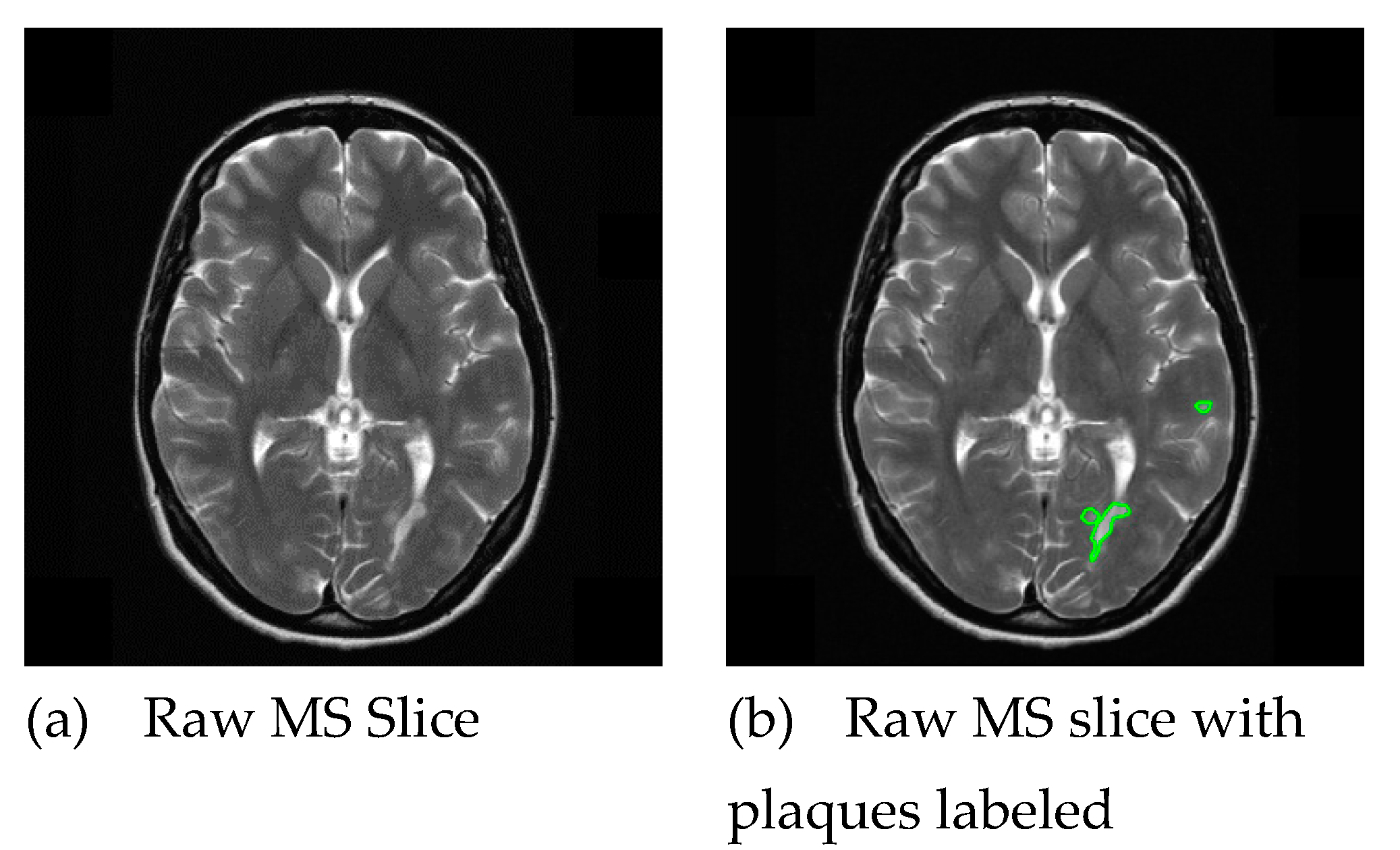
2. Dataset
3. Methodology
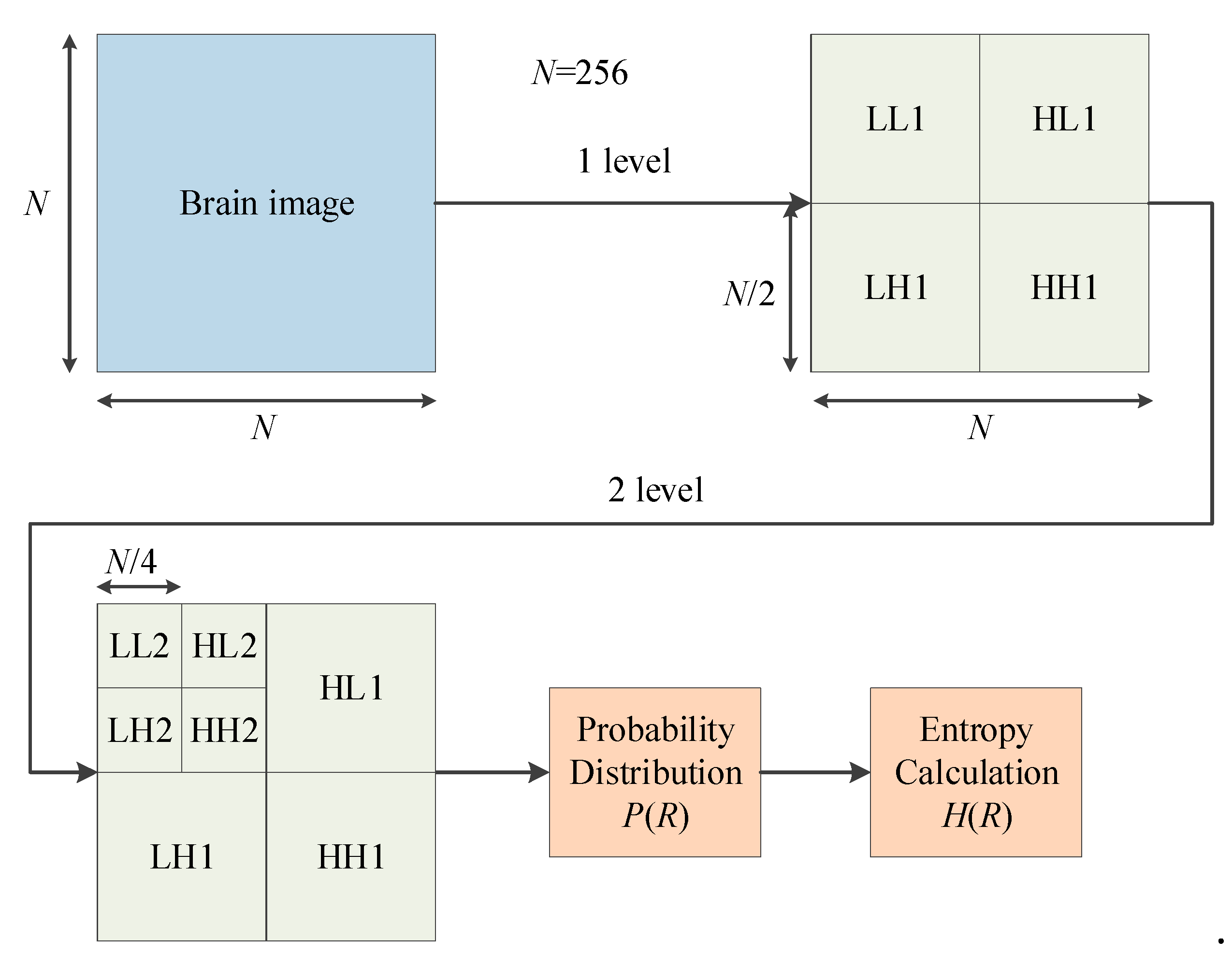
3.1. Wavelet Entropy
- Step 1: Wavelet Transform
- Step 2: Probability Distribution
- Step 3: Entropy Calculation
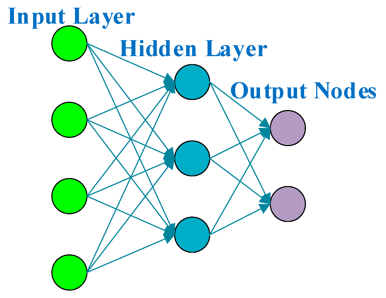
3.2. Feedforward Neural Network
3.3. PSO-Based Neural Network
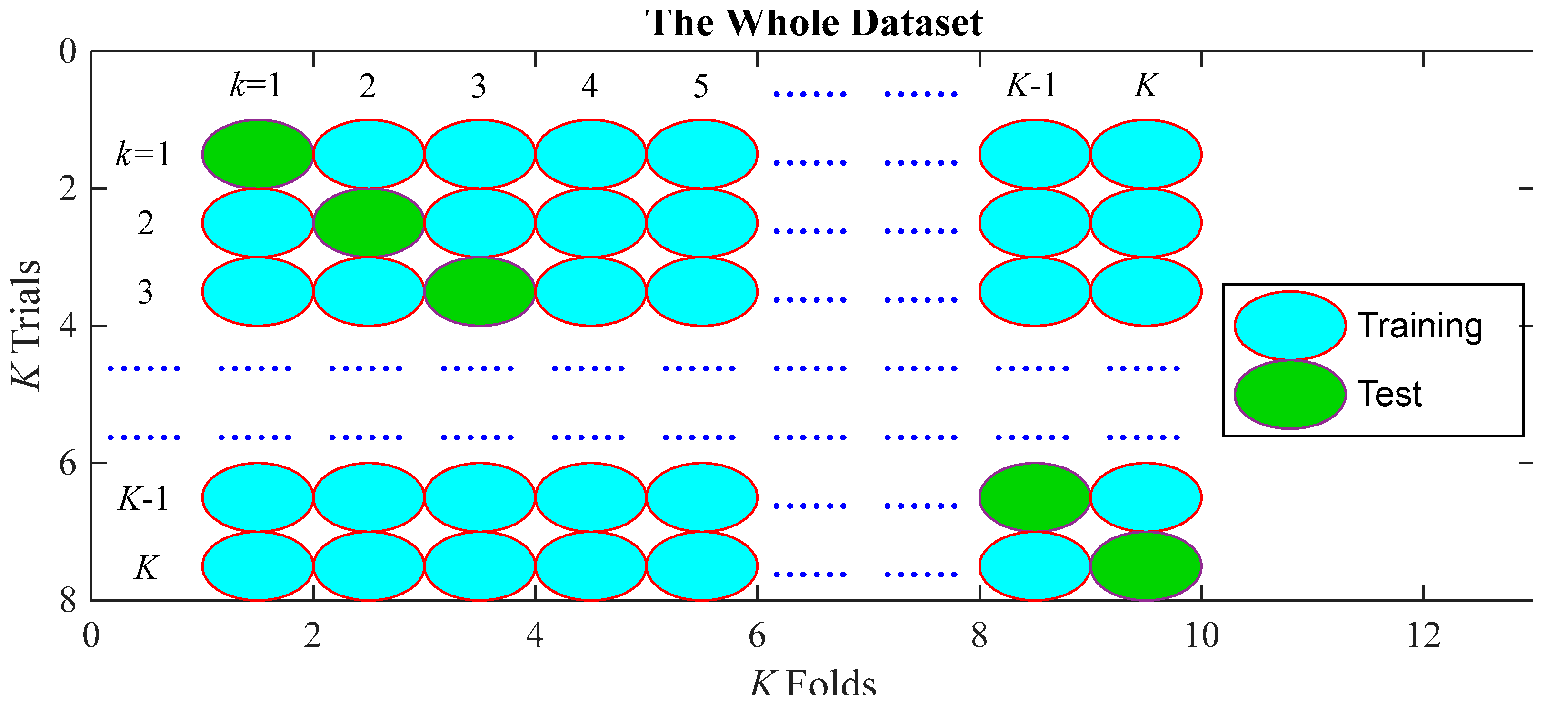
3.4. 10-Fold Cross Validation
3.5. Measure on runs
4. Results and Discussions
4.1. Statistical Analysis
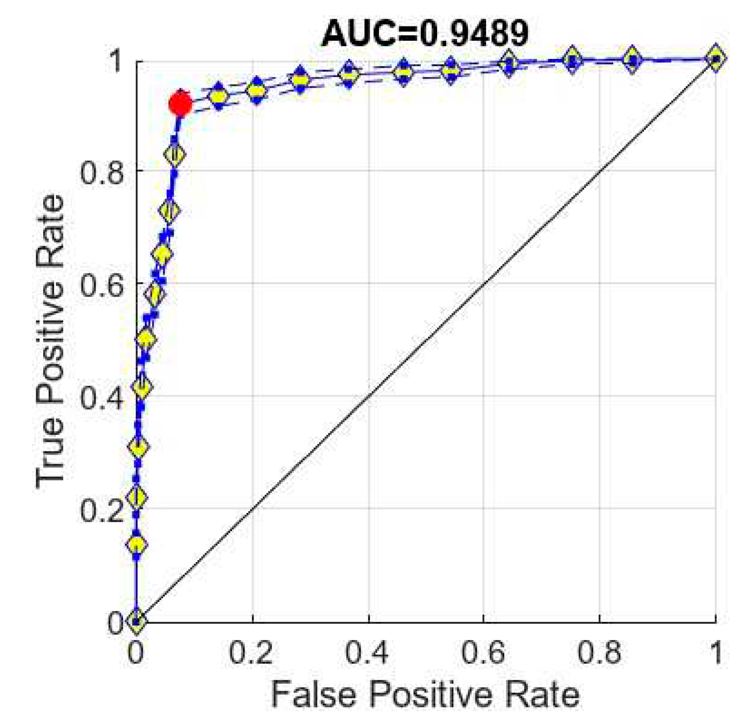
4.2. ROC Curve
4.3. PSO versus AGA
4.4. Comparison with State-of-the-Art Algorithms
5. Conclusions
Funding
Acknowledgment
Conflict of Interest
References
- Kornbluh, A.B.; Kahn, I. Pediatric Multiple Sclerosis. Semin. Pediatr. Neurol. 2023, 46, 101054. [Google Scholar] [CrossRef] [PubMed]
- Quigley, S.; Asad, M.; Doherty, C.; Byrne, D.; Cronin, S.; Kearney, H. Concurrent diagnoses of Tuberous sclerosis and multiple sclerosis. Mult. Scler. Relat. Disord. 2023, 71, 104586. [Google Scholar] [CrossRef] [PubMed]
- Maroto-García, J.; Martínez-Escribano, A.; Delgado-Gil, V.; Mañez, M.; Mugueta, C.; Varo, N.; de la Torre. G.; Ruiz-Galdón, M. Biochemical biomarkers for multiple sclerosis. Clin. Chim. Acta 2023, 548, 117471. [Google Scholar] [CrossRef] [PubMed]
- Chagot, C.; Vlaicu, M.B.; Frismand, S.; Colnat-Coulbois, S.; Nguyen, J.P.; Palfi, S. Deep brain stimulation in multiple sclerosis-associated tremor. A large, retrospective, longitudinal open label study, with long-term follow-up. Mult. Scler. Relat. Disord. 2023, 79, 104928. [Google Scholar] [CrossRef] [PubMed]
- Lunin, S.; Novoselova, E.; Glushkova, O.; Parfenyuk, S.; Kuzekova, A.; Novoselova, T.; Sharapov, M.; Mubarakshina, E.; Goncharov, R.; Khrenov, M. Protective effect of exogenous peroxiredoxin 6 and thymic peptide thymulin on BBB conditions in an experimental model of multiple sclerosis. Arch. Biochem. Biophys. 2023, 746, 109729. [Google Scholar] [CrossRef]
- E Freedman, D.; Krysko, K.M.; Feinstein, A. Intimate partner violence and multiple sclerosis. Mult. Scler. J. 2023. [Google Scholar] [CrossRef] [PubMed]
- Cerri, S.; Hoopes, A.; N. Greve, D.; Muhlau, M.; Van Leemput, K. A Longitudinal Method for Simultaneous Whole-Brain and Lesion Segmentation in Multiple Sclerosis. Arxiv 2020, arXiv:2008.05117, doi:arXiv:2008.05117.
- Atapour, M.; Maghaminejad, F.; Ghiyasvandian, S.; Rahimzadeh, M.; Hosseini, S. The psychometric properties of the Persian version of the Multiple Sclerosis Self-Management Scale-Revised: A cross-sectional methodological study. Heal. Sci. Rep. 2023, 6, e1515. [Google Scholar] [CrossRef]
- Shafiee, A.; Soltani, H.; Athar, M.M.T.; Jafarabady, K.; Mardi, P. The prevalence of depression and anxiety among Iranian people with multiple sclerosis: A systematic review and meta-analysis. Mult. Scler. Relat. Disord. 2023, 78, 104922. [Google Scholar] [CrossRef]
- Eisler, J.J.; Disanto, G.; Sacco, R.; Zecca, C.; Gobbi, C. Influence of Disease Modifying Treatment, Severe Acute Respiratory Syndrome Coronavirus 2 Variants and Vaccination on Coronavirus Disease 2019 Risk and Outcome in Multiple Sclerosis and Neuromyelitis Optica. J. Clin. Med. 2023, 12, 5551. [Google Scholar] [CrossRef]
- Turčić, A.; Radovani, B.; Vogrinc. ; Habek, M.; Rogić, D.; Gabelić, T.; Zaninović, L.; Lauc, G.; Gudelj, I. Higher MRI lesion load in multiple sclerosis is related to the N-glycosylation changes of cerebrospinal fluid immunoglobulin G. Mult. Scler. Relat. Disord. 2023, 79, 104921. [Google Scholar] [CrossRef] [PubMed]
- Karaaslan, Z.; Şengül-Yediel, B.; Yüceer-Korkmaz, H.; Şanlı, E.; Gezen-Ak, D.; Dursun, E.; Timirci-Kahraman. ; Baykal, A.T.; Yılmaz, V.; Türkoğlu, R.; et al. Chloride intracellular channel protein-1 (CLIC1) antibody in multiple sclerosis patients with predominant optic nerve and spinal cord involvement. Mult. Scler. Relat. Disord. 2023, 78, 104940. [Google Scholar] [CrossRef]
- Chisari, C.G.; Guadagno, J.; Adjamian, P.; Silvan, C.V.; Greco, T.; Bagul, M.; Patti, F. A post hoc evaluation of the shift in spasticity category in individuals with multiple sclerosis-related spasticity treated with nabiximols. Ther. Adv. Neurol. Disord. 2023, 16. [Google Scholar] [CrossRef] [PubMed]
- Zhang, Y.; Yang, J.; Wang, S.; Dong, Z.; Phillips, P. Pathological brain detection in MRI scanning via Hu moment invariants and machine learning. J. Exp. Theor. Artif. Intell. 2016, 29, 299–312. [Google Scholar] [CrossRef]
- Lasalvia, M.; Gallo, C.; Capozzi, V.; Perna, G. Discrimination of Healthy and Cancerous Colon Cells Based on FTIR Spectroscopy and Machine Learning Algorithms. Appl. Sci. 2023, 13, 10325. [Google Scholar] [CrossRef]
- Kiyak, E.O.; Ghasemkhani, B.; Birant, D. High-Level K-Nearest Neighbors (HLKNN): A Supervised Machine Learning Model for Classification Analysis. Electronics 2023, 12, 3828. [Google Scholar] [CrossRef]
- Han, G.; Wang, Y.; Liu, J.; Zeng, F. Low-light images enhancement and denoising network based on unsupervised learning multi-stream feature modeling. J. Vis. Commun. Image Represent. 2023, 96. [Google Scholar] [CrossRef]
- Liu, X.; Li, Z. Dynamic multiple access based on deep reinforcement learning for Internet of Things. Comput. Commun. 2023, 210, 331–341. [Google Scholar] [CrossRef]
- Wu, X.; Lopez, M. Multiple Sclerosis Slice Identification by Haar Wavelet Transform and Logistic Regression. Advances in Materials, Machinery, Electrical Engineering (AMMEE 2017). LOCATION OF CONFERENCE, ChinaDATE OF CONFERENCE.
- Han, J.; Hou, S.-M. Multiple Sclerosis Detection via Wavelet Entropy and Feedforward Neural Network Trained by Adaptive Genetic Algorithm. International Work-Conference on Artificial Neural Networks. LOCATION OF CONFERENCE, SpainDATE OF CONFERENCE; pp. 87–97.
- Zhao, Y.; Chitnis, T. Dirichlet Mixture of Gaussian Processes with Split-kernel: An Application to Predicting Disease Course in Multiple Sclerosis Patients. 2022 International Joint Conference on Neural Networks (IJCNN). LOCATION OF CONFERENCE, ItalyDATE OF CONFERENCE; pp. 1–8.
- Han, J.; Hou, S.-M. A Multiple Sclerosis Recognition via Hu Moment Invariant and Artificial Neural Network Trained by Particle Swarm Optimization. International Conference on Multimedia Technology and Enhanced Learning. LOCATION OF CONFERENCE, United KingdomDATE OF CONFERENCE; pp. 254–264.
- MRI Lesion Segmentation in Multiple Sclerosis Database. eHealth laboratory, University of Cyprus, 2021.
- Zhang, Y.-D.; Pan, C.; Sun, J.; Tang, C. Multiple sclerosis identification by convolutional neural network with dropout and parametric ReLU. J. Comput. Sci. 2018, 28, 1–10. [Google Scholar] [CrossRef]
- Gleason, J.L.; Tamburro, R.; Signore, C. Promoting Data Harmonization of COVID-19 Research in Pregnant and Pediatric Populations. JAMA 2023, 330, 497–498. [Google Scholar] [CrossRef] [PubMed]
- Norris, C.J.; Kim, S. A Use Case of Iterative Logarithmic Floating-Point Multipliers: Accelerating Histogram Stretching on Programmable SoC. 2023 IEEE International Symposium on Circuits and Systems (ISCAS). LOCATION OF CONFERENCE, United StatesDATE OF CONFERENCE; pp. 1–5.
- Wang, S.-H.; Sun, J.; Phillips, P.; Zhao, G.; Zhang, Y.-D. Polarimetric synthetic aperture radar image segmentation by convolutional neural network using graphical processing units. J. Real-Time Image Process. 2017, 15, 631–642. [Google Scholar] [CrossRef]
- Dwivedi, D.; Chamoli, A.; Rana, S.K. Wavelet Entropy: A New Tool for Edge Detection of Potential Field Data. Entropy 2023, 25, 240. [Google Scholar] [CrossRef]
- Hua, F.; Ling, T.; He, W.; Liu, X. Wavelet Entropy-Based Method for Migration Imaging of Hidden Microcracks by Using the Optimal Wave Velocity. Int. J. Pattern Recognit. Artif. Intell. 2022, 36. [Google Scholar] [CrossRef]
- Wang, S.; Li, Y.; Shao, Y.; Cattani, C.; Zhang, Y.; Du, S. Detection of Dendritic Spines Using Wavelet Packet Entropy and Fuzzy Support Vector Machine. CNS Neurol. Disord. - Drug Targets 2017, 16, 116–121. [Google Scholar] [CrossRef]
- Wang, J.J. COVID-19 Diagnosis by Wavelet Entropy and Particle Swarm Optimization. Proceedings of 18th International Conference on Intelligent Computing (ICIC), Xian, PEOPLES R CHINA, Aug 07-11; pp. 600–611.
- Janani, A.S.; Rezaeieh, S.A.; Darvazehban, A.; Keating, S.E.; Abbosh, A.M. Portable Electromagnetic Device for Steatotic Liver Detection Using Blind Source Separation and Shannon Wavelet Entropy. IEEE J. Electromagn. Rf Microwaves Med. Biol. 2022, 6, 546–554. [Google Scholar] [CrossRef]
- Tao, Y.; Scully, T.; Perera, A.G.; Lambert, A.; Chahl, J. A Low Redundancy Wavelet Entropy Edge Detection Algorithm. J. Imaging 2021, 7, 188. [Google Scholar] [CrossRef] [PubMed]
- Valluri, D.; Campbell, R. ; Ieee. On the Space of Coefficients of a Feedforward Neural Network. In Proceedings of International Joint Conference on Neural Networks (IJCNN), Broadbeach, AUSTRALIA, Jun 18-23.
- Yotov, K.; Hadzhikolev, E.; Hadzhikoleva, S.; Cheresharov, S. A Method for Extrapolating Continuous Functions by Generating New Training Samples for Feedforward Artificial Neural Networks. Axioms 2023, 12, 759. [Google Scholar] [CrossRef]
- Zhang, Y.; Wu, L. Improved image filter based on SPCNN. Sci. China Inf. Sci. 2008, 51, 2115–2125. [Google Scholar] [CrossRef]
- Admon, M.R.; Senu, N.; Ahmadian, A.; Majid, Z.A.; Salahshour, S. A new efficient algorithm based on feedforward neural network for solving differential equations of fractional order. Commun. Nonlinear Sci. Numer. Simul. 2023, 117. [Google Scholar] [CrossRef]
- Abernot, M.; Delacour, C.; Suna, A.; Gregg, J.M.; Karg, S.; Todri-Sanial, A. Two-Layered Oscillatory Neural Networks with Analog Feedforward Majority Gate for Image Edge Detection Application. 2023 IEEE International Symposium on Circuits and Systems (ISCAS). LOCATION OF CONFERENCE, United StatesDATE OF CONFERENCE; pp. 1–5.
- Sharma, S.; Achlerkar, P.D.; Shrivastava, P.; Garg, A.; Panigrahi, B.K. Combined SoC and SoE Estimation of Lithium-ion Battery using Multi-layer Feedforward Neural Network. 2022 IEEE International Conference on Power Electronics, Drives and Energy Systems (PEDES). LOCATION OF CONFERENCE, IndiaDATE OF CONFERENCE; pp. 1–6.
- Le, X.-K.; Wang, N.; Jiang, X. Nuclear mass predictions with multi-hidden-layer feedforward neural network. Nucl. Phys. A 2023, 1038. [Google Scholar] [CrossRef]
- Yurtkan, K.; Adalier, A.; Tekgüç, U. Student Success Prediction Using Feedforward Neural Networks. Romanian J. Inf. Sci. Technol. 2023, 2023, 121–136. [Google Scholar] [CrossRef]
- Wang, S.-H.; Zhang, Y.-D. Advances and Challenges of Deep Learning. Recent Patents Eng. 2022. [Google Scholar] [CrossRef]
- Zhou, J. Logistics inventory optimization method for agricultural e-commerce platforms based on a multilayer feedforward neural network. Pakistan Journal of Agricultural Sciences 2023, 60, 487–496. [Google Scholar] [CrossRef]
- Ben Braiek, H.; Khomh, F. Testing Feedforward Neural Networks Training Programs. ACM Trans. Softw. Eng. Methodol. 2023, 32, 1–61. [Google Scholar] [CrossRef]
- R, S.; Sheshappa, S.N.; Vijayakarthik, P.; Raja, S.P. Global Pattern Feedforward Neural Network Structure with Bacterial Foraging Optimization towards Medicinal Plant Leaf Identification and Classification. Int. J. Adv. Comput. Sci. Appl. 2022, 13. [Google Scholar] [CrossRef]
- Bidyanath, K.; Singh, S.D.; Adhikari, S. Implementation of genetic and particle swarm optimization algorithm for voltage profile improvement and loss reduction using capacitors in 132 kV Manipur transmission system. Energy Rep. 2023, 9, 738–746. [Google Scholar] [CrossRef]
- Karami, M.R.; Jaleh, B.; Eslamipanah, M.; Nasri, A.; Rhee, K.Y. Design and optimization of a TiO2/RGO-supported epoxy multilayer microwave absorber by the modified local best particle swarm optimization algorithm. Nanotechnol. Rev. 2023, 12. [Google Scholar] [CrossRef]
- S. Wang, "Magnetic resonance brain classification by a novel binary particle swarm optimization with mutation and time-varying acceleration coefficients," Biomedical Engineering-Biomedizinische Technik, vol. 61, pp. 431-441, 2016.
- Ghaeb, J.; Al-Naimi, I.; Alkayyali, M. Intelligent Integrated Approach for Voltage Balancing Using Particle Swarm Optimization and Predictive Models. J. Electr. Comput. Eng. 2023, 2023, 1–14. [Google Scholar] [CrossRef]
- Karpat, E.; Imamoglu, F. Optimization and Comparative Analysis of Quarter-Circular Slotted Microstrip Patch Antenna Using Particle Swarm and Fruit Fly Algorithms. Int. Arab. J. Inf. Technol. 2023, 20, 624–631. [Google Scholar] [CrossRef]
- Katipoğlu, O.M.; Yeşilyurt, S.N.; Dalkılıç, H.Y.; Akar, F. Application of empirical mode decomposition, particle swarm optimization, and support vector machine methods to predict stream flows. Environ. Monit. Assess. 2023, 195, 1–21. [Google Scholar] [CrossRef]
- Wang, S.-H.; Wu, X.; Zhang, Y.-D.; Tang, C.; Zhang, X. Diagnosis of COVID-19 by Wavelet Renyi Entropy and Three-Segment Biogeography-Based Optimization. Int. J. Comput. Intell. Syst. 2020, 13, 1332–1344. [Google Scholar] [CrossRef]
- de Sousa, I.A.; Reis, I.A.; Pagano, A.S.; Telfair, J.; Torres, H.d.C. Translation, cross-cultural adaptation and validation of the sickle cell self-efficacy scale (SCSES). Hematol. Transfus. Cell Ther. 2023, 45, 290–296. [Google Scholar] [CrossRef] [PubMed]
- Yu, Q.; Guo, J.; Gong, F. Construction and Validation of a Diagnostic Scoring System for Predicting Active Pulmonary Tuberculosis in Patients with Positive T-SPOT Based on Indicators Associated with Coagulation and Inflammation: A Retrospective Cross-Sectional Study. Infect. Drug Resist. 2023, ume 16, 5755–5764. [Google Scholar] [CrossRef]
- Ton, V. Validation of a mathematical model of ultrasonic cross-correlation flow meters based on industrial experience. Flow Meas. Instrum. 2023, 93. [Google Scholar] [CrossRef]
- Mahmood, Q.K.; Jalil, A.; Farooq, M.; Akbar, M.S.; Fischer, F. Development and validation of the Post-Pandemic Fear of Viral Disease scale and its relationship with general anxiety disorder: a cross-sectional survey from Pakistan. BMC Public Heal. 2023, 23, 1739. [Google Scholar] [CrossRef] [PubMed]
- Liyanage, V.; Tao, M.; Park, J.S.; Wang, K.N.; Azimi, S. Malignant and non-malignant oral lesions classification and diagnosis with deep neural networks. J. Dent. 2023, 137, 104657. [Google Scholar] [CrossRef] [PubMed]
- Ivanov, I.G.; Kumchev, Y.; Hooper, V.J. An Optimization Precise Model of Stroke Data to Improve Stroke Prediction. Algorithms 2023, 16, 417. [Google Scholar] [CrossRef]
- Bansal, S.; Gowda, K.; Kumar, N. Multilingual personalized hashtag recommendation for low resource Indic languages using graph-based deep neural network. Expert Syst. Appl. 2024, 236. [Google Scholar] [CrossRef]
- Abirami, L.; Karthikeyan, J. Digital Twin-Based Healthcare System (DTHS) for Earlier Parkinson Disease Identification and Diagnosis Using Optimized Fuzzy Based k-Nearest Neighbor Classifier Model. IEEE Access 2023, 11, 96661–96672. [Google Scholar] [CrossRef]
- Alkawsi, G.; Al-Amri, R.; Baashar, Y.; Ghorashi, S.; Alabdulkreem, E.; Tiong, S.K. Towards lowering computational power in IoT systems: Clustering algorithm for high-dimensional data stream using entropy window reduction. Alex. Eng. J. 2023, 70, 503–513. [Google Scholar] [CrossRef]
- Dejene, M.; Palanivel, H.; Senthamarai, H.; Varadharajan, V.; Prabhu, S.V.; Yeshitila, A.; Benor, S.; Shah, S. Optimisation of culture conditions for gesho (Rhamnus prinoides.L) callus differentiation using Artificial Neural Network-Genetic Algorithm (ANN-GA) Techniques. Appl. Biol. Chem. 2023, 66, 1–14. [Google Scholar] [CrossRef]
- Nakamura, H.; Zhang, J.; Hirose, K.; Shimoyama, K.; Ito, T.; Kanaumi, T. Generating simplified ammonia reaction model using genetic algorithm and its integration into numerical combustion simulation of 1 MW test facility. Appl. Energy Combust. Sci. 2023, 15. [Google Scholar] [CrossRef]
- Zhang, Y.; Wang, S.; Huo, Y.; Wu, L.; Liu, A. FEATURE EXTRACTION OF BRAIN MRI BY STATIONARY WAVELET TRANSFORM AND ITS APPLICATIONS. J. Biol. Syst. 2010, 18, 115–132. [Google Scholar] [CrossRef]
- Chen, Y.; Yu, Q.; Lu, Y. Pulsar Timing Array Detections of Supermassive Binary Black Holes: Implications from the Detected Common Process Signal and Beyond. Astrophys. J. 2023, 955, 132. [Google Scholar] [CrossRef]
- Zhou, C.R.; Wang, Z.T.; Yang, S.W.; Xie, Y.H.; Liang, P.; Cao, D.; Chen, Q. Application Progress of Chemometrics and Deep Learning Methods in Raman Spectroscopy Signal Processing. Chinese Journal of Analytical Chemistry 2023, 51, 1232–1242. [Google Scholar] [CrossRef]
- Kolhar, M.; Aldossary, S.M. Privacy-Preserving Convolutional Bi-LSTM Network for Robust Analysis of Encrypted Time-Series Medical Images. AI 2023, 4, 706–720. [Google Scholar] [CrossRef]
- Wu, D.; Li, L.; Wang, J.; Ma, P.; Wang, Z.; Wu, H. Robust zero-watermarking scheme using DT CWT and improved differential entropy for color medical images. J. King Saud Univ. - Comput. Inf. Sci. 2023, 35. [Google Scholar] [CrossRef]
- Zhang, Y.-D.; Wang, S.-H.; Yang, X.-J.; Dong, Z.-C.; Liu, G.; Phillips, P.; Yuan, T.-F. Pathological brain detection in MRI scanning by wavelet packet Tsallis entropy and fuzzy support vector machine. SpringerPlus 2015, 4, 1–16. [Google Scholar] [CrossRef]
- Shandilya, S.K.; Srivastav, A.; Yemets, K.; Datta, A.; Nagar, A.K. YOLO-based segmented dataset for drone vs. bird detection for deep and machine learning algorithms. Data Brief 2023, 50, 109355. [Google Scholar] [CrossRef]
| Category | NS | NS | Gender (m/f) | Age |
|---|---|---|---|---|
| MS [23] | 38 | 676 | 17/21 | 34.1 ± 10.5 |
| HC [24] | 26 | 681 | 12/14 | 33.5 ± 8.3 |
| Run | |||||||
|---|---|---|---|---|---|---|---|
| 1 | 92.60 | 91.63 | 91.65 | 92.11 | 92.13 | 84.23 | 92.13 |
| 2 | 90.38 | 90.90 | 90.79 | 90.64 | 90.59 | 81.28 | 90.59 |
| 3 | 93.05 | 93.83 | 93.74 | 93.44 | 93.39 | 86.88 | 93.39 |
| 4 | 90.68 | 93.10 | 92.88 | 91.89 | 91.77 | 83.81 | 91.77 |
| 5 | 90.09 | 91.34 | 91.17 | 90.71 | 90.62 | 81.43 | 90.63 |
| 6 | 92.46 | 92.66 | 92.59 | 92.56 | 92.52 | 85.11 | 92.52 |
| 7 | 92.75 | 92.51 | 92.48 | 92.63 | 92.61 | 85.26 | 92.61 |
| 8 | 93.20 | 92.80 | 92.78 | 93.00 | 92.99 | 86.00 | 92.99 |
| 9 | 91.86 | 92.80 | 92.69 | 92.34 | 92.27 | 84.67 | 92.27 |
| 10 | 92.46 | 92.07 | 92.05 | 92.26 | 92.25 | 84.53 | 92.25 |
| MSD | 91.95±1.15 | 92.36±0.88 | 92.28±0.88 | 92.16±0.90 | 92.11±0.92 | 84.32±1.79 | 92.12±0.91 |
| Method | |||||||
|---|---|---|---|---|---|---|---|
| AGA [20] | 91.91±1.24 | 91.98±1.36 | 91.97±1.32 | 91.95±1.19 | 91.92±1.20 | 83.89±2.41 | 91.92±1.19 |
| PSO (Ours) | 91.95±1.15 | 92.36±0.88 | 92.28±0.88 | 92.16±0.90 | 92.11±0.92 | 84.32±1.79 | 92.12±0.91 |
| Method | |||||||
|---|---|---|---|---|---|---|---|
| LR [19] | 89.63±1.75 | 90.48±1.45 | 90.34±1.43 | 90.06±1.44 | 89.98±1.47 | 80.13±2.87 | 89.98±1.47 |
| DMGPS [21] | 88.99±1.20 | 88.56±1.13 | 88.54±1.05 | 88.78±0.95 | 88.76±0.96 | 77.56±1.91 | 88.77±0.96 |
| HMI [22] | 91.67±1.41 | 91.73±0.77 | 91.70±0.78 | 91.70±0.97 | 91.67±1.00 | 83.40±1.98 | 91.67±0.99 |
| WE-PSONN (Ours) | 91.95±1.15 | 92.36±0.88 | 92.28±0.88 | 92.16±0.90 | 92.11±0.92 | 84.32±1.79 | 92.12±0.91 |
Disclaimer/Publisher’s Note: The statements, opinions and data contained in all publications are solely those of the individual author(s) and contributor(s) and not of MDPI and/or the editor(s). MDPI and/or the editor(s) disclaim responsibility for any injury to people or property resulting from any ideas, methods, instructions or products referred to in the content. |
© 2023 by the authors. Licensee MDPI, Basel, Switzerland. This article is an open access article distributed under the terms and conditions of the Creative Commons Attribution (CC BY) license (http://creativecommons.org/licenses/by/4.0/).


