1. Introduction
Consider the linear matrix equation
where
,
and
. Such problems arise in linear control and filtering theory for continuous or discrete-time large-scale dynamical systems. If
is consistent,
is the minimum Frobenius norm solution. If
is inconsistent,
is the minimum Frobenius norm least squares solution. When the matrices
A and
B are small and dense, direct methods based on QR-fraction are attractive [
1,
2]. However, for large matrices
A and
B, iterative methods have attracted much attention [
3,
4,
5,
6,
7]. Recently, Du et al. proposed the randomized block coordinate descent (RBCD) method for solving the matrix least-squares problem
without strong convexity assumption in [
8]. This method requires that matrix
B is full row rank. Wu et al. [
9] introduced two kinds of Kaczmarz-type methods to solve consistent matrix equation
: relaxed greedy randomized Kaczmarz (ME-RGRK) and maximal weighted residual Kaczmarz (ME-MWRK). Although the row and column index selection strategy is time-consuming, the ideas of these two methods are suitable for solving large-scale consistent matrix equations.
In this paper, randomized Kaczmarz method [
10] and randomized extended Kaczmarz method [
11] are used to solve consistent and inconsistent matrix equations (
1) by the product of matrix and vector.
All the results in this paper hold in the complex field. But for the sake of simplicity, we only discuss it in the real number field.
In this paper, we denote , , , , and as the transpose, the Moore-Penrose generalized inverse, the rank of A, the column space of A, the Frobenius norm of A and the inner product of two matrices A and B, respectively. For an integer , let . We use I to denote the identity matrix whose order is clear from the context. In addition, for a given matrix , , , and , are used to denote ith row, jth column, the maximum singular value and the smallest nonzero singular value of G respectively. Let denote the expected value conditional on the first k iterations, that is, where and are the row and the column chosen at the sth iteration. Let the conditional expectations with respect to the random row index be and with respect to the random column index be By the law of total expectation, it holds that .
The organization of this paper is as follows. In
Section 2, we will discuss Kaczmarz method (ME-RBK and ME-PRBK) for finding the minimal
F-norm solution (
) of the consistent matrix Eq. (
1). In
Section 3, we discuss the extended Kaczmarz method (IME-REBK) for finding the minimal
F-norm least-squares solution of the matrix Eq. (
1). In
Section 4, some numerical examples are provided to illustrate the effectiveness of our new methods. Finally, some brief concluding remarks are described in
Section 5.
2. The Randomized Block Kaczmarz Method for Consistent Equation
At the
kth iteration, Kaczmarz method selects randomized a row
of
A and does an orthogonal projection of the current estimate matrix
onto the corresponding hyperplane
, that is
The Lagrangian function of the conditional optimization problem (
2) is
where
is Lagrangian multiplier. By the matrix differentiation, we get the gradient of
and set
for finding the stationary matrix:
By the first equation of (
4), we have
. Substituting this into the second equation of (
4), we can get
. So the projected randomized block Kacmarz (ME-PRBK) for solving
iterates as
However, in practice, it is very expensive to calculate the pseudoinverse of large-scale matrices. Next, we generalize the average block Kaczmarz method [
12] for solving linear equations to matrix equations.
At the
kth step, we get the approximate solution
by projecting the current estimate
onto the hyperplane
. Using the Lagrangian multiplier method, we can obtain the following Kaczmarz method for
:
Inspired by the idea of average block Kaczmaz algorithm for
, we consider the average block Kaczmaz method for
respect to
B.
where
is stepsize and
be the weights that satisfy
and
. If
, then
Set
, we obtain the following randomized block Kaczmarz iteration
where
i is selected with probability
. The cost of each iteration of this method is
if the square of the row norm of
A has been calculated in advance. We describe this method as Algorithm 1, which is called the ME-RBK algorithm.
Remark 1.
Note that the problem of finding a solution of can be posed as the following linear least squares problem
Define the component function
then differentiate with X to get its gradient
Therefore, the randomized block Kaczmarz method (9) is equivalent to one step of the stochastic gradient decent method [13] applied to (10) with stepsize .
First, we give the following lemma whose proof can be found in [
8].
Lemma 1.
[8] Let and be any nonzero matrix. Let
For any matrix , it holds
Remark 2. means that and . In fact, is well defined because and .
In the following theorem, with the idea of the RK method [
10], we will prove that Algorithm 1 converges to the the least
F-norm solution of
.
Theorem 1.
Assume . If Eq. (1) is consistent, the sequence generated by the ME-RBK method starting from the initial matrix in which and , converges linearly to in mean square form. Moreover, the solution error in expectation for the iteration sequence obeys
where , and picked with probability .
Proof. For
, by (
9) and
(consistency), we have
then
By taking the conditional expectation, we have
By
and
, we have
. Noting
, it is easy to show that
by induction. Then by Lemma 1 and
, we can get
Finally, by ((
12)) and induction on the iteration index
k, we obtain the estimate ((
11)). □
Remark 3.
By the similar approach as used in the proof of Theorem 1, we can prove that the iterate generated by ME-PRBK (5) satisfies the following estimate
where . The convergence factor of GRK in [14] is . It is obvious that
and when . This means that the convergence factor of ME-PRBK is the smallest and the factor of ME-RBK can be smaller than that of GRK when α is properly selected.
3. The Randomized Extended Block Kaczmarz Method for Inconsistent Equation
In [
11,
15,
16], the authors proved that the Kaczmarz method does not converge to the least squares solution of
when
is inconsistent. Analogically, if the matrix Eq. (
1) is inconsistent, the above ME-PRBK method dose not converge to
. The following theorem give the error bound of the for the inconsistent matrix equation.
Theorem 2.
Assume that the consistent equation has a solution . Let denote the kth iterate of the ME-PRBK method applied to the inconsistent for any starting from the initial matrix in which and . In exact arithmetic, it follows that
Proof. Set
,
. Let
Y denote the iterate of the PRBK method applied to the consistent
at
kth step, that is
By taking the conditional expectation on both sides of (
14), we can obtain
The inequality is obtained by Remark 3. Applying this recursive relation iteratively, we have
This completes the proof. □
Next, we use the idea of randomized extended Kaczmarz method (see [
16,
17,
18] for details) for solving the least squares solution of the inconsistent Eq. (
1). At each iteration,
is the
kth iterate of ME-RBK applied to
with the initial guess
, and
is one-step ME-RBK update for
. we can get the following randomized extended block Kaczmarz iteration
where
is the step size, and
i and
j are selected with probability
and
, respectively. The cost of each iteration of this method is
for updating
and
for updating
if the square of the row norm and the column norm of
A have been calculated in advance. We describe this method as Algorithm 2, which is called the ME-REBK algorithm.

Theorem 3.
Assume . Let denote the kth iterate of ME-RBK applied to starting from the initial matrix in which and . Then converges linearly to in mean square form, and the solution error in expectation for the iteration sequence obeys
where the jth column of A is selected with probability .
Proof. The approach of proof is the same as that used in the proof of Theorem 1, so we omit it. □
Theorem 4.
Assume . The sequence is generated by the ME-REBK method for starting from the initial matrix and , where , and . For any , it holds
where , are picked with probability and , respectively.
Proof. Let
denote the
kth iterate of ME-REBK method for
, and
be the one-step Kaczmarz update for the matrix equation
from
, i.e.,
For any
, by triangle inequality and Young’s inequality, we can get
By taking the conditional expectation on the both sides of (
18), we have
By
, we have
. Then, by using Theorem 1, we can get
then
Combining (
19),(
20) and (
21) yields
This completes the proof. □
Remark 4.
Replacing in (15) with , we obtain the following projection-based randomized extended block Kaczmarz mathod (ME-PREBK) iteration
4. Numerical Experiments
In this section, we will present some experiment results of the proposed algorithms for solving various matrix equations, and compare them with ME-RGRK and ME-MWRK in [
9] for consistent matrix equations and RBCD in [
8] for inconsistent matrix equations. All experiments are carried out by using MATLAB (version R2020a) on a DESKTOP-8CBRR86 with Intel(R) Core(TM) i7-4712MQ CPU @2.30GHz 2.29GHz, RAM 8GB and Windows 10.
All computations are started from the initial guess
, the step size
, and terminated once the relative error (RE) of the solution, defined by
at the the current iterate
, satisfies
or exceeds maximum iteration
, where
. We report the average number of iterations (denoted as “IT”) and the average computing time in seconds (denoted as“CPU”) for 20 trials repeated runs of the corresponding method. Three examples are tested, and
A and
B are generated as follows.
Type I: For given , the entries of A and B are generated from a standard normal distribution, i.e.,
Type II: Like [
14], for given
, and
, we construct a matrix
A by
, where
and
are orthogonal columns matrices,
is a diagonal matrix whose first
diagonal entries are uniformly distributed numbers in
, and the last two diagonal entries are
. The entries of
B are generated by similar method with parameters
.
Type III: The real-world sparse data come from the Florida sparse matrix collection [
19].
4.1. Consistent Matrix Equation
Given
, we set
with
to construct a consistent matrix equation. In
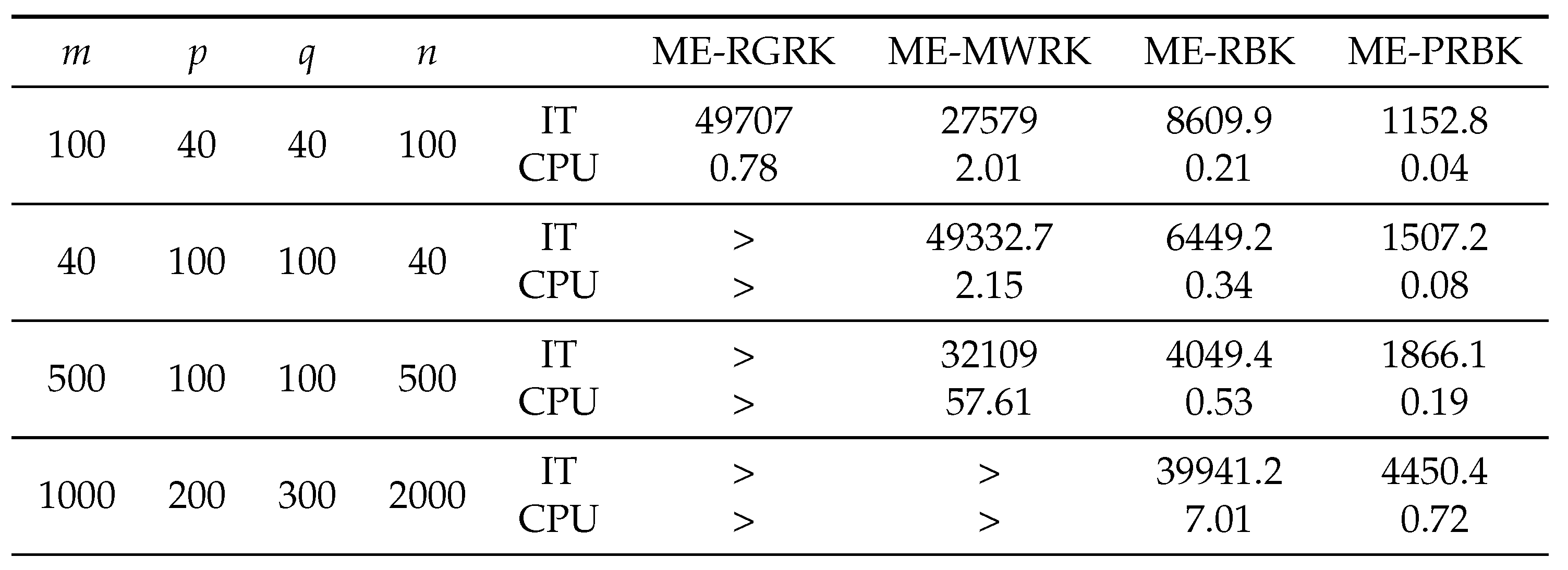
Table 1,
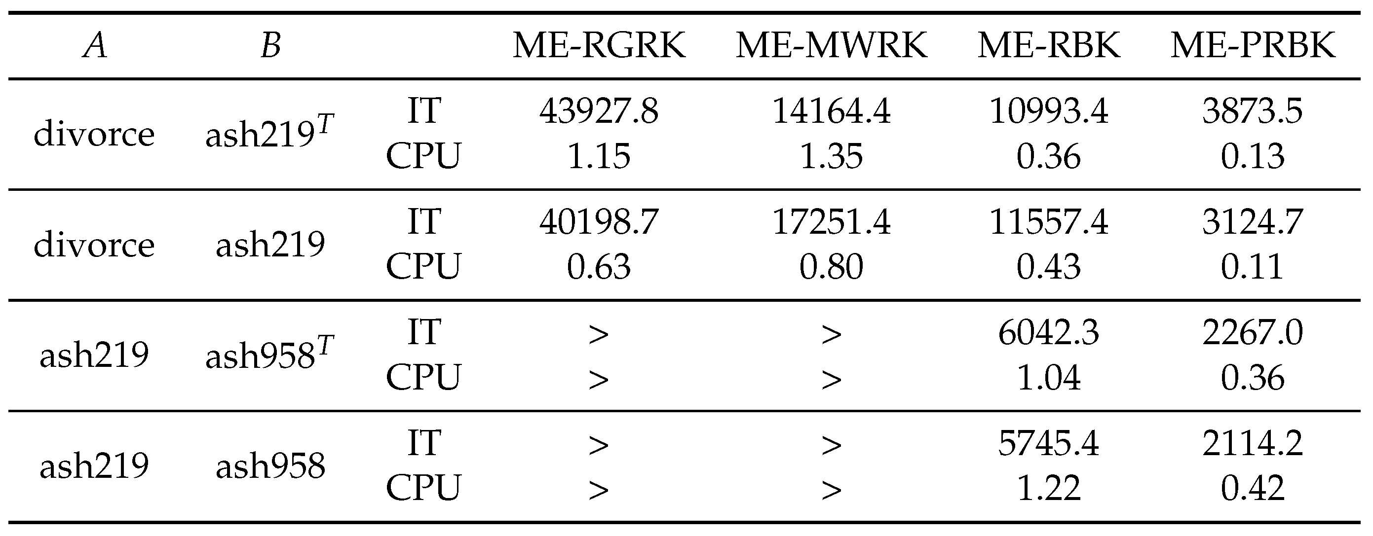
Table 2 and
Table 3, we report the average IT and CPU of the ME-RGRK, ME-MWRK, ME-RBK and ME-PRBK methods for solving consistent matrix. In the following tables, the item `>’ represents that the number of iteration steps exceeds the maximum iteration (50000), and the item `-’ represents that the method does not converge.
From these tables, we can see that the ME-RBK and ME-PRBK methods vastly outperform the ME-RGRK and ME-MWRK methods in terms of both IT and CPU times regardless of whether the matrices A and B are full column/row rank or not. As the increasing of matrix dimension, the CPU time of ME-RBK and ME-PRBK methods is increasing slowly , while the running time of ME-RGRK and ME-MWRK increases dramatically.
In addition, when the matrix size is small, the ME-PRBK method is competitive, because of the pseudoinverse is less expensive and the number of iteration steps is small. When the matrix size is large, the matrix is large, the ME-RBK method is more challenging because it does not need to calculate the pseudoinverse (see the last line in
Table 1).
4.2. Inonsistent Matrix Equation
To construct an inconsistent matrix equation, we set
, where
and
R are random matrices which are generated by
and
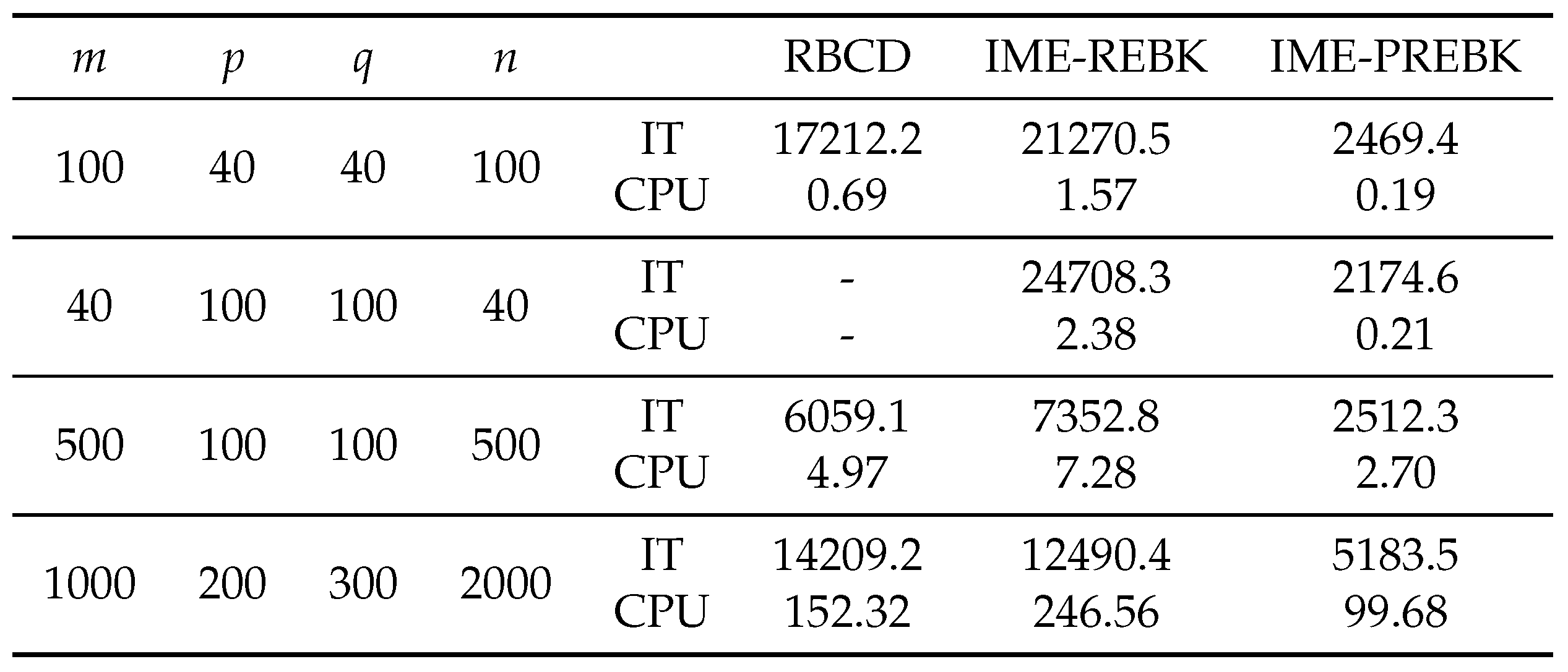
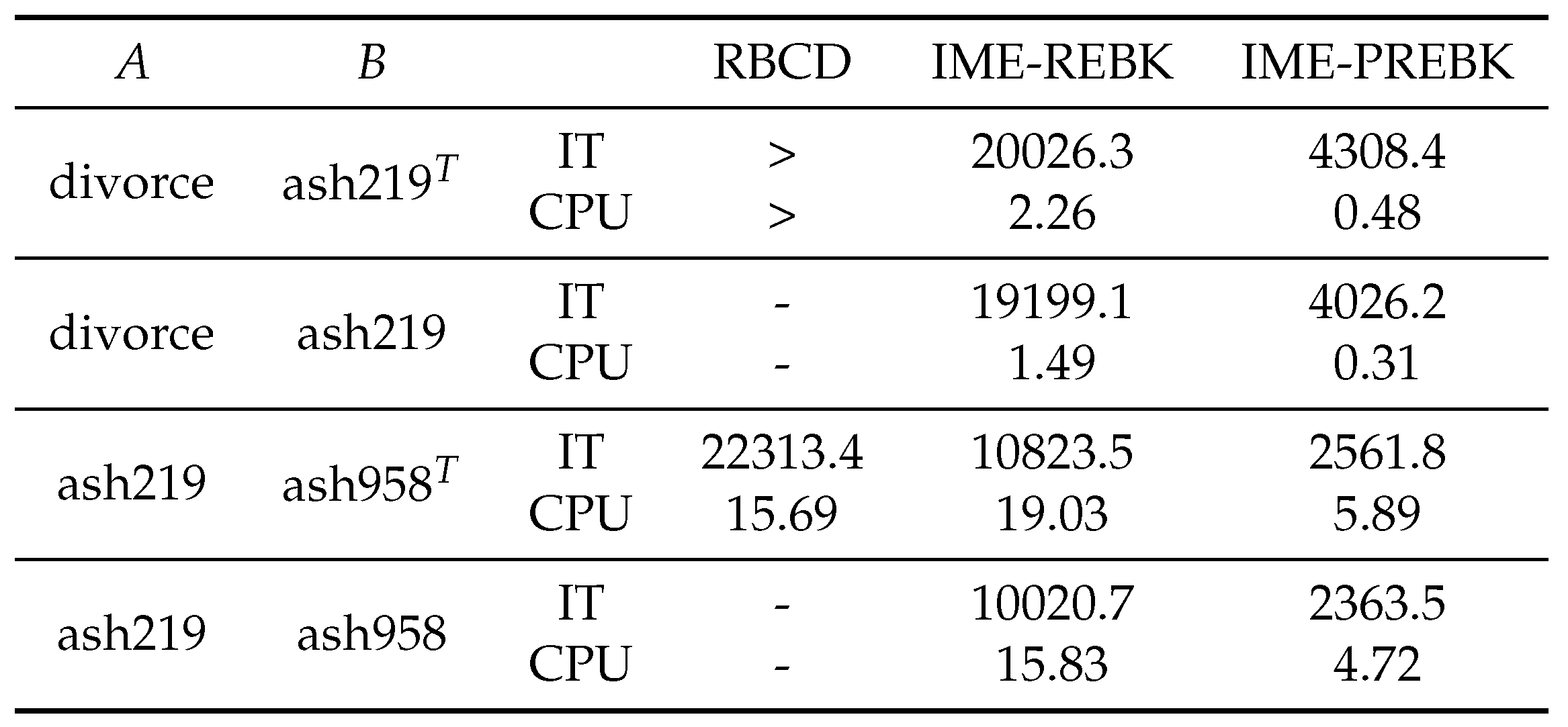
. Numerical results of the RBCD, IME-REBK and IME-PREBK methods are listed in
Table 4,
Table 5 and
Table 6. From these tables, we can see that the IME-PREBK method is better than the RBCD method in terms of IT and CPU time, especially when the
is large (see the last line in
Table 5). The IME-REBK method is not competitive for B with full row rank because it needs to solve two equations. However, when B has not full row rank, the RBCD method does not converge, while the IME-REBK and IME-PREBK methods do.
5. Conclusions
In this paper we have proposed a randomized block Kaczmarz algorithm for solving the consistent matrix equation and its extended version for the inconsistent case. Theoretically, we have proved the proposed algorithms converge linearly to the unique minimal F-norm solution or least-squares solution (i.e., ) without requirements on A and B have full column/row rank. Numerical results show the effectiveness of the algorithms. Since the proposed algorithms only require one row or one column of A at each iteration without matrix-matrix product, it is suitable for the scenarios where the matrix A is too large to fit in memory or matrix multiplication is considerably expensive.
Author Contributions
Conceptualization, L.X.; Methodology, L.X. and W.B.; Validation, L.X. and W.L.; Writing—original draft preparation, L.X.; Writing—review and editing, L.X., W.B and W.L.; Software, L.X.; Visualization, L.X. and W.L. All authors have read and agreed to the published version of the manuscript
Funding
This research received no external funding.
Institutional Review Board Statement
The authors declare that they have no known competing financial interests or personal relationships that could have appeared to influence the work reported in this paper.
Data Availability Statement
The datasets that support the findings of this study are available from the corresponding author upon reasonable request.
Acknowledgments
The authors are thankful to the referees for their constructive comments and valuable suggestions, which have greatly improved the original manuscript of this paper.
Conflicts of Interest
The authors declare no conflict of interest.
References
- Fausett, D.W.; Fulton, C.T. Large least squares problems involving Kronecker products. SIAM J. Matrix Anal. Appl. 1994, 15, 219–227. [Google Scholar] [CrossRef]
- Zha, H.Y. Comments on large least squares problems involving Kronecker products. SIAM J. Matrix Anal. Appl. 1995, 16, 1172–1172. [Google Scholar] [CrossRef]
- Peng, Z.Y. An iterative method for the least squares symmetric solution of the linear matrix equation AXB = C. Appl. Math. Comput. 2005, 170, 711–723. [Google Scholar] [CrossRef]
- Ding, F.; Liu, P.X.; Ding, J. Iterative solutions of the generalized Sylvester matrix equations by using the hierarchical identification principle. Appl. Math. Comput. 2008, 197, 41–50. [Google Scholar] [CrossRef]
- Huang, G.X.; Yin, F.; Guo, K. An iterative method for the skew-symmetric solution and the optimal approximate solution of the matrix equation AXB = C. J. Comput. Appl. Math. 2008, 212, 231–244. [Google Scholar] [CrossRef]
- Wang, X.; Li, Y.; Dai, L. On hermitian and skew-hermitian splitting iteration methods for the linear matrix equation AXB = C. Comput. Math. Appl. 2013, 65, 657–664. [Google Scholar] [CrossRef]
- Shafiei, S.G.; Hajarian, M. Developing Kaczmarz method for solving Sylvester matrix equations. J. Franklin Inst. 2022, 359, 8991–9005. [Google Scholar] [CrossRef]
- Du, K.; Ruan, C.C.; Sun, X.H. On the convergence of a randomized block coordinate descent algorithm for a matrix least squaress problem. Appl. Math. Lett. 2022, 124, 107689. [Google Scholar] [CrossRef]
- Wu, N.C.; Liu, C.Z.; Zuo, Q. On the Kaczmarz methods based on relaxed greedy selection for solving matrix equation AXB=C. J. Comput. Appl. Math. 2022, 413, 114374. [Google Scholar] [CrossRef]
- Strohmer, T.; Vershynin, R. A randomized Kaczmarz algorithm with exponential convergence. J Fourier Anal. Appl. 2009, 15, 262–278. [Google Scholar] [CrossRef]
- Zouzias, A.; Freris, N.M. Randomized extended Kaczmarz for solving least squares. SIAM J Matrix Anal Appl. 2013, 34, 773–793. [Google Scholar] [CrossRef]
- Ion, N. Faster randomized block kaczmarz algorithms. SIAM J. Matrix Anal. Appl. 2019, 40, 1425–1452. [Google Scholar]
- Nemirovski, A.; Juditsky, A.; Lan, G.; Shapiro, A. Robust stochastic approximation approach to stochastic programming. SIAM J. Optimiz. 2009, 19, 1574–1609. [Google Scholar] [CrossRef]
- Niu, Y.Q.; Zheng, B. On global randomized block Kaczmarz algorithm for solving large-scale matrix equations. arXiv 2204, arXiv:2204.13920. [Google Scholar]
- Needell, D. Randomized Kaczmarz solver for noisy linear systems. BIT Numer Math. 2010, 50, 395–403. [Google Scholar] [CrossRef]
- Ma, A.; Needell, D. A. Ramdas, Convergence properties of the randomized extended Gauss-Seidel and Kaczmarz methods. SIAM J. Matrix Anal. Appl. 2015, 36, 1590–1604. [Google Scholar] [CrossRef]
- Du, K. Tight upper bounds for the convergence of the randomized extended Kaczmarz and Gauss-Seidel algorithms. Numer. Linear Algebra Appl. 2019, 26, e2233. [Google Scholar] [CrossRef]
- Du, K.; Si, W.T.; Sun, X.H. Randomized extended average block kaczmarz for solving least squares. SIAM J. Sci. Comput. 2020, 42, A3541–A3559. [Google Scholar] [CrossRef]
- Davis, T.A.; Hu, Y. The university of Florida sparse matrix collection. Math. Softw. 2011, 38, 1–25. [Google Scholar] [CrossRef]
Table 1.
IT and CPU of ME-RGRK, ME-MWRK, ME-RBK and ME-PRBK for the consistent matrix equations with Type I.
Table 1.
IT and CPU of ME-RGRK, ME-MWRK, ME-RBK and ME-PRBK for the consistent matrix equations with Type I.
Table 2.
IT and CPU of ME-RGRK, ME-MWRK, ME-RBK and ME-PRBK for the consistent matrix equations with Type II.
Table 2.
IT and CPU of ME-RGRK, ME-MWRK, ME-RBK and ME-PRBK for the consistent matrix equations with Type II.
Table 3.
IT and CPU of ME-RGRK, ME-MWRK, ME-RBK and ME-PRBK for the consistent matrix equations with Type III.
Table 3.
IT and CPU of ME-RGRK, ME-MWRK, ME-RBK and ME-PRBK for the consistent matrix equations with Type III.
Table 4.
IT and CPU of RBCD, IME-REBK and IME-PREBK for the inconsistent matrix equations with Type I.
Table 4.
IT and CPU of RBCD, IME-REBK and IME-PREBK for the inconsistent matrix equations with Type I.
Table 5.
IT and CPU of RBCD, IME-REBK and IME-PREBK for the inconsistent matrix equations with Type II.
Table 5.
IT and CPU of RBCD, IME-REBK and IME-PREBK for the inconsistent matrix equations with Type II.
Table 6.
IT and CPU of RBCD, IME-REBK and IME-PREBK for the inconsistent matrix equations with Type III.
Table 6.
IT and CPU of RBCD, IME-REBK and IME-PREBK for the inconsistent matrix equations with Type III.
|
Disclaimer/Publisher’s Note: The statements, opinions and data contained in all publications are solely those of the individual author(s) and contributor(s) and not of MDPI and/or the editor(s). MDPI and/or the editor(s) disclaim responsibility for any injury to people or property resulting from any ideas, methods, instructions or products referred to in the content. |
© 2023 by the authors. Licensee MDPI, Basel, Switzerland. This article is an open access article distributed under the terms and conditions of the Creative Commons Attribution (CC BY) license (http://creativecommons.org/licenses/by/4.0/).


