EDDformer: A New Decoder for Efficient Semantic Segmentation of Remote Sensing Urban Scene Imagery

Preprint

Article

EDDformer: A New Decoder for Efficient Semantic Segmentation of Remote Sensing Urban Scene Imagery

Altmetrics

Downloads

105

Views

Comments

Bing Liu,Yansheng Gao,

Tongye Hu,

Hongwei Zhao^*

Bing Liu,Yansheng Gao,

Tongye Hu,

Hongwei Zhao^*

This version is not peer-reviewed

Submitted:

10 October 2023

Posted:

11 October 2023

You are already at the latest version

Alerts

Abstract

Semantic segmentation of remote sensing urban scene imagery is a pixel-wise prediction, which is applied to identify the land-cover or land-use category. However, semantic segmentation demands huge computation cost. In order to reduce the huge computation cost, a common method is to introduce transformer and CNN hybrid method to have a good trade-off between accuracy and computation cost. However, recent CNN-transformer hybrid methods often capture local-global context and cross-window interaction information simultaneously. Then they introduce the local-global context to fuse the local feature, which repeat fuse the local and global feature and result in the additional computation cost. And previous methods often ignore to filter the local and global feature. To fix the problem, we design a lightweight decoder-EDDformer, which is Efficient Global Value Transformer with Dynamic Gatefusion module. Efficient global value transformer only response for extracting global feature. Dynamic Gatefusion module filter the local and global semantic feature and fuse them to capture the local-global context in one time. Extensive experiments reveal that our method not only runs faster but also achieves higher accuracy compared with other state-of-the-art lightweight models.

Keywords:

Subject: Computer Science and Mathematics - Artificial Intelligence and Machine Learning

1. Introduction

Semantic segmentation of remote sensing urban scene imagery plays a important role in the urban-related applications [1], such as land cover mapping [2,3], change detection [4], environment protection [5], and building extraction [6]. With the development of deep-learning based methods. The CNN has dominated the semantic segmentation. Compared with some traditional machine learning based methods (e.g., SVM, CRF. random forest), CNN-based [7] methods can extract the more fine-grained feature with inductive bias. Such as Unet [8], which first proposes a end-to-end methods to fix the semantic segmentation. BiSeNet [9] designs a lightweight CNN model to fix the semantic segmentation. ABCNet [10] introduces a two path architecture to capture the local-global context. More and more CNN-based methods have shown that CNN have more powerful representation ability.

However, the CNN-based methods introduce convolution to extract local feature, which can not capture the contextual information of image. Therefore, the lack of contextual information can not leads semantic segmentation can not recognition the pixel with same class accurately. In order to fix the problem, the transformer of NLP field raise the attention of computer vision field. The self-attention mechanism can encoder the global contextual information effectively. Therefore, numerous transformer-based methods are proposed to capture contextual information. Such as Segmenter [11], which seems patches as token and capture the contextual information of these tokens. Segformer [12] introduces a transformer-based decoder to extract multi-scale semantic feature to fix the semantic segmentation. However, the huge dimension of remote sensing imagery results in the numerous computation cost, which limit the application of self-attention for real-time urban applications. And the attention mechanism have not the capacity of inductive bias. The lack of detail information often leads the ambiguity of pixels.

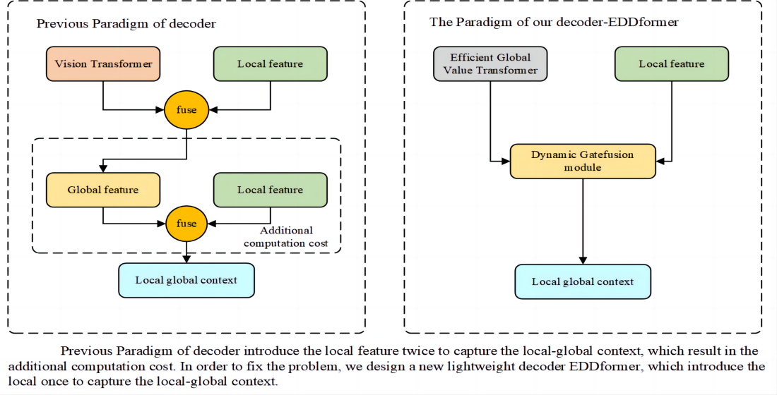
To fix the problem of the convolution and self-attention. A common method is to combine the CNN and vision transformer. Such as UNetformer [13], which introduces a CNN-based encoder and transformer-based decoder to extract the local and global feature and fuse them to get the local-global context. However, previous methods often capture the local-global context in the transformer module. Then they fuse the local-global context with local feature to inject the detail information. The way to extract local-global context and inject detail information introduce the local feature twice, which results in the additional computation cost. And they often ignore to filter the local feature and global feature, which will result in the semantic gap.

In order to fix above problems, our goal is to design a lightweight decoder, which only introduce local feature once to get the local-global context. And we also want to filter the local and global feature in the process of the using of local feature. Therefore, we propose a new decoder-EDDformer Efficient Global Value Transformer, Dynamic Gatefusion (DGF) Module and Dynamic refine head (DRHead). The Efficient Global Value Transformer consists of Global Value Window Self-attention (GVWSA) module and a MLP head, which only responsible for extracting global feature. And our proposed GVWSA module can add the interaction information of spatial and channel dim. The DGF Module introduces the gating mechanism to produce the gate for filtering the local feature and global feature. And the DGF Module only introduce the local feature once to fuse the local and global feature to get the local-global context. Besides all, we design DRHead to refine the feature for the better final prediction.

Extensive experiments show that our methods can achieve the state-of-the-art performance in the LoveDA [14], UAVid [15], Vaihingen [16], and Potsdam [17] datasets while lower computation cost. We also conduct numerous ablation studies to prove the effectiveness of our proposed modules.

In summary, our contribution can be listed as follows:

1. We design a lightweight decoder EDDformer, which reduce the computation cost by introducing local feature once to capture the local-global context.

2. We propose Efficient Value Window Self-attention (GVWSA) module, which extracts the global context and add interaction information in the spatial and channel dim.

3. We propose Dynamic Gatefusion (DGF) module to filter and fuse the local and global feature to capture local-global context.

4. We design Dynamic Refine Head (DRHead) to refine the local-global context dynamic to better predict the final segmentaion map.

5. We outperform the existing state-of-the-art efficient semantic segmentation models and achieve a good trade-off between computational cost and accuracy on 4 widely used benchmark datasets: loveda, vaihingen, potsdam, and Uavid.

2. Related Work

Efficient semantic segmentation of remote sensing images: The real world application of remote sensing technology requires a lightweight model to fix the semantic segmentation. Therefore, the CNN-based [7] methods have dominated the semantic segmentation of remote sensing images due to the powerful capacity of feature extracting and low computation cost of convolution operation. Such as FCN [18], which introduce a CNN encoder and upsample the feature to fix the semantic segmentation. The Unet [8] introduces the encoder the downsample the feature gradually and use deconvolution and skip-connection to upsample and inject the detail information. However, the limited receptive fields results in the low accuracy, which limit the application of real world remote sensing technology. To fix the problem, transformer-based [19] methods are proposed to capture the global context. The self-attention mechanism has the global receptive field. However, the huge dimension of remote sensing images result in the huge computation cost. Therefore, some careful designed methods are propose to reduce the computation cost. Such as Swin transformer [20], which introduces shifted window self-attention to reduce the computation cost. Cross transformer [20] introduces the criss self-attention to reduce the computation cost. Even though the way they compute the self-attention reduce the computation cost largely. They still have the large computation cost and lack of the ability of inductive bias. In order to take advantage of CNN and transformer, CNN-transformer hybrid methods are proposed to fix the semantic segmentation of remote sensing images. Such as UNetformer [13], which introduce a CNN encoder and transformer-based decoder to extract the local and global feature, respectively. And the transformer-based decoder also response for capturing the local-global context by fusing the local and global feature. However, the way the capture the local-global context introduce the local feature twice, which results in the inevitable computation cost. To fix the problem, we propose EDDformer, which introduce local feature once to capture the local-global context.

lightweight Vision Transformer decoder: Recently, the encoder-decoder architecture has been a typical way to fix the semantic segmentation. However, the limited receptive field are difficult to capture the global context. Therefore, many works focus on to design a lightweight vision transformer decoder to capture the global context and have a good trade-off between accuracy and computation cost. Such as Segmenter [11], which simple introduce a pure transformer-based decoder to conduct self-attention on patch tokens. Segformer [12] designs a transformer-based decoder to extract the multi-scale global semantic feature and upsample the segmentation map for the final prediction. However, all of the previous methods introduce the vallina self-attention to capture the global context, which result in the large computation cost. And all of the previous methods often fail the filter the local and global feature. Different with these methods, our proposed transformer-based decoder introduce our proposed Efficient Global Value Transformer to capture the global context with lower computation cost. And in order to filter the local and global feature, we propose dynamic gating fusion (DGF) module, which introduce gating mechanism to filter the local and global feature.

Gating Mechanism: The gating mechanism is first proposed in the Recurrent neural networks [21] of NLP fields. The LSTM [22] and GRU [23] are the first gating mechanism to control the passing of information. Recently, the gating mechanism has been widely used in the CV field. Such as GateNet [24], which introduces feature embedding and hidden gates the capture the high-order interaction information. GFF [25] selected the features from different scales. In this paper, we propose dynamic gating fusion module, which introduce sigmoid activation function to product gate for filtering feature.

3. Methods

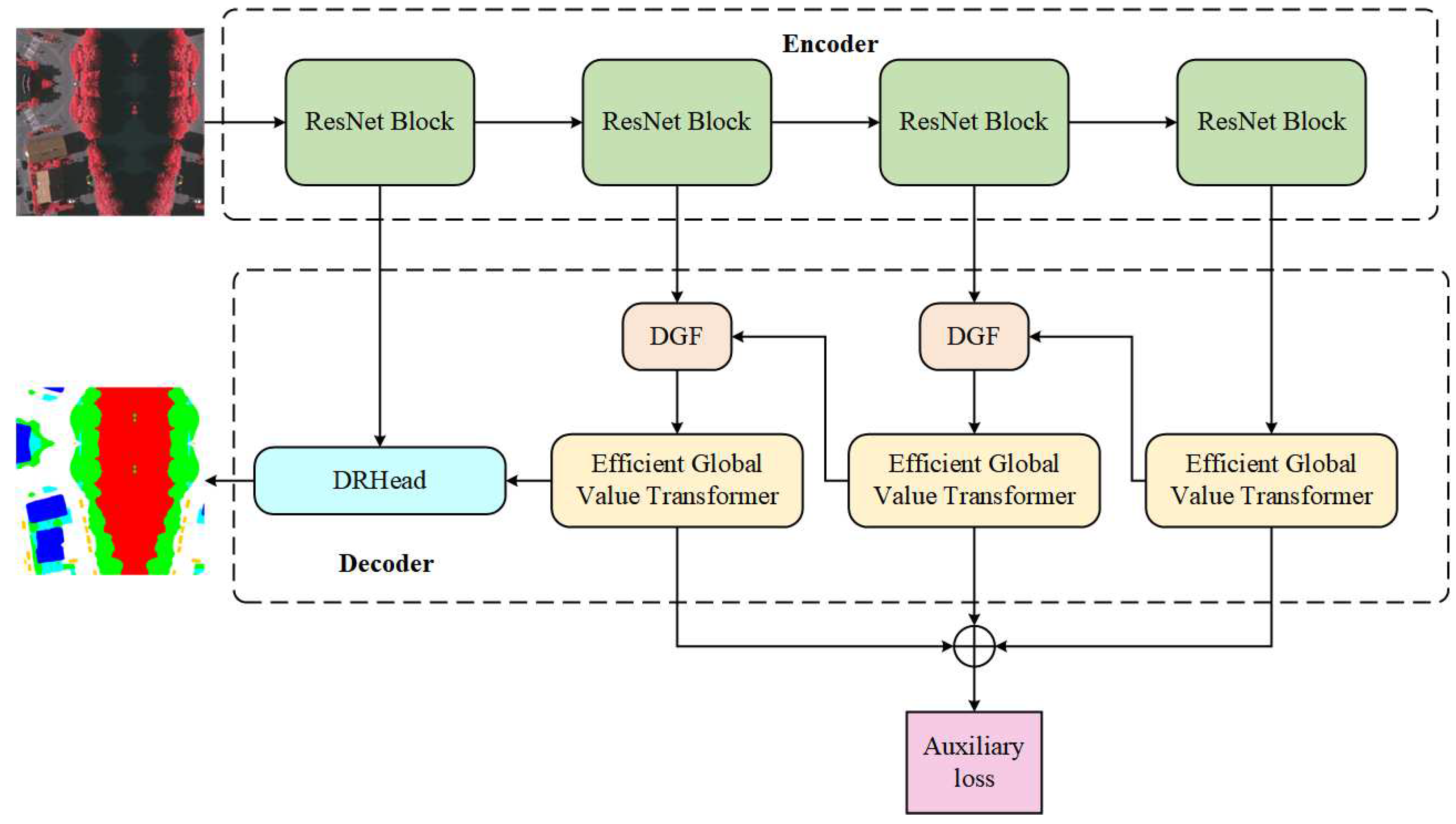
As shown in the Figure 1, our GVDformer consists a encoder and a decoder. The encoder is a typical ResNet backbone, which consists of four stages CNN blocks. The encoder is used to extract the local feature. The decoder is a lightweight decoder, which consists of Efficient Global Value Transformer (GVformer), Dynamic Gatefusion (DGF) module, and Dynamic Refine Head (DRHead). A detail instruction of each module is given in the follow sections. The Efficient Global Value Transformer first capture the global context. Then we introduce DGF module to fuse the global and local feature to capture the local-global context. Finally we introduce the DRHead to fine-grain the local-global context for the better prediction.

3.1. Encoder

As shown in the Figure 1, our encoder is a four-stage ResNet backbone. And we choose the vallina ResNet18 [26] as our encoder, which has been proved that the effectiveness and efficiently for the semantic segmentation. Formally, we seem the image

I \in R^{H \times W \times C}

as the input of encoder. The

H, W, c

mean height, width, and channel, respectively. And we feed the I to the four stage ResNet backbone. And we can get the output of local feature

L_{i}, {i = 1, 2, 3, 4}

. i is the stage number. The whole process of encoder can be written as:

L_{i} = L_{i - 1} + R e s B l o c k (L_{i - 1}), i = 1, 2, 3, 4

(1)

where i is the stage number,

R e s B l o c k ()

is the vallina ResNet block. The process of ResNet block can be written as:

R e s B l o c k (x) = C o n v 3 (C o n v 2 (C o n v 1 (x)))

(2)

The X is the input of the ResNet block. The

C o n v 1

C o n v 2

, and the

C o n v 3

are the

3 \times 3

convolution. After throughing the ResNet backbone, we can get the local feature

L_{i}

. And the dimension of

L_{i}

L_{1} \in R^{\frac{H}{4} \times \frac{W}{4} \times 64}

L_{2} \in R^{\frac{H}{8} \times \frac{W}{8} \times 128}

L_{3} \in R^{\frac{H}{16} \times \frac{W}{16} \times 256}

L_{4} \in R^{\frac{H}{32} \times \frac{W}{32} \times 512}

Figure 1. The overall architecture of our proposed EDDformer.

3.2. Decoder

As shown in the Figure 1, our decoder seems the outputs of encoder

L_{i}

as the input of decoder. We first introduce a

1 \times 1

convolution to adjust the channel number of

L_{4}

to 64. Then we feed the

L_{4}

to the Efficient Global Value Transformer to capture the global context

G_{i}, {i = 1, 2, 3}

. After we get the global context

G_{i}

, we seems

G_{i}

and

L_{i}

{i = 1, 2, 3}

as the input of DGF to filter the local and global feature and get the local-global context efficiently. Finally, we introduce the DRHead to refine the local-global context. That’s the way to introduce local feature once to capture and refine the local-global context. By this way, we can achieve a good trade-off between accuracy and computation cost. The whole process of decoder can be written as:

G_{i} = G V F o r m e r (L_{i})

(3)

F_{l g} = D G F (G_{i}, L_{i})

(4)

F_{l g}^{f} = D R H (F_{l g})

(5)

where i is the stage number,

G V F o r m e r (.)

is our proposed GVformer,

D G F

and

D R H

are our proposed Dynamic gating fusion module and Dynamic refine head, respectively.

L_{i}

and

G_{i}

are the local feature and global feature, respectively.

F_{l g}

and

F_{l g}^{f}

are the local-global context and fine-grained local-global context, respectively.

A detailed description of each part in decoder is given in the following sections.

3.2.1. Efficient Global Value Transformer

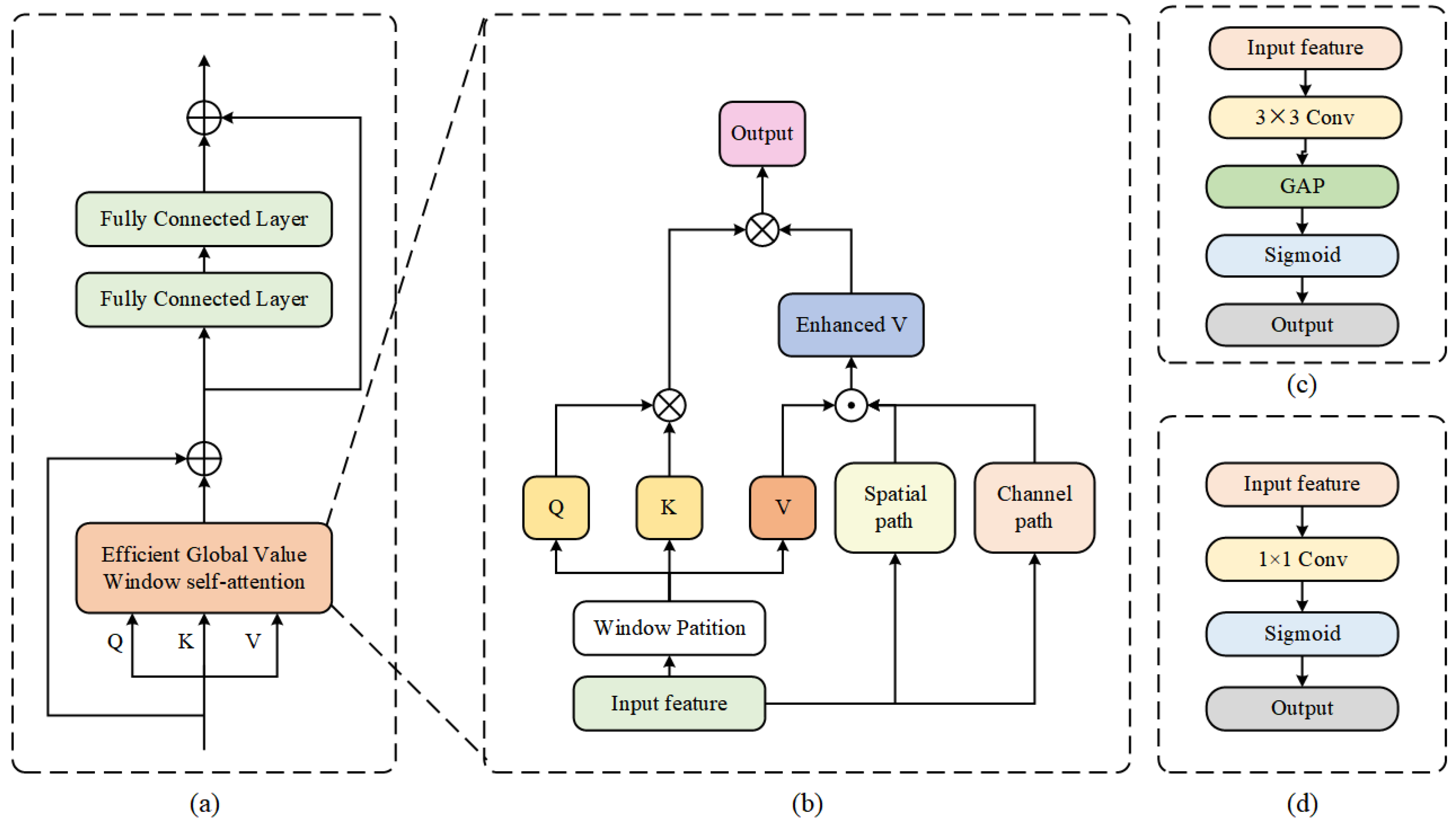
As shown in the Figure 2, our Efficient Global Value Transformer consists of Efficient Value Window Self-attention module and MLP head. The Efficient Value window Self-attention can capture the global context and add the cross-window interaction information in the channel and spatial dim into the value.

As shown in the Figure 2b, our proposed GVWSA introduces window self-attention to capture global context. And our GVWSA introduces spatial path and channel path to get the enhanced V, which means value with cross-window interaction information. Formally, the process can be written as:

V_{e} = v \cdot S P (L_{i}) \cdot C P (L_{i})

(6)

where

S P

means spatial path and

C P

means channel path. The

V_{e}

and

L_{i}

stands for the enhanced v and the local feature of stage i, which is the input of Efficient Global Value Window self-attention.

After we get the

V_{e}

, we introduce the multi head window self-attention, the calculation can be written as:

G V W S A M (Q, K, V_{e}) = C o n c a t (T_{o u t}^{0}, . . . ., T_{o u t}^{j}) W^{p r o j}

(7)

T_{o u t}^{j} = A t t e n t i o n (Q^{j}, K^{j}, V_{e}^{j})

(8)

where

C o n c a t ()

is the concatenate operation,

W^{p r o j}

means the projection head in self-attention, GVWSAM means Global Value Window self-attention. j means the head number.

Q^{j}

K^{j}

, and

V_{e}^{j}

means query, key,and enhanced value of the jth head.

Similar with the self-attention, the attention operation can be written as:

A t t e n t i o n (q, k, v) = S o f t m a x (\frac{q k^{T}}{\sqrt{d}}) v

(9)

where d is the dimension of heads.

For the MLP, we simple introduce two fully connected layer as the MLP head. And the architecture of spatial path and channel path are shown in the Figure 2c,d.

3.2.2. Dynamic Gatefusion Module

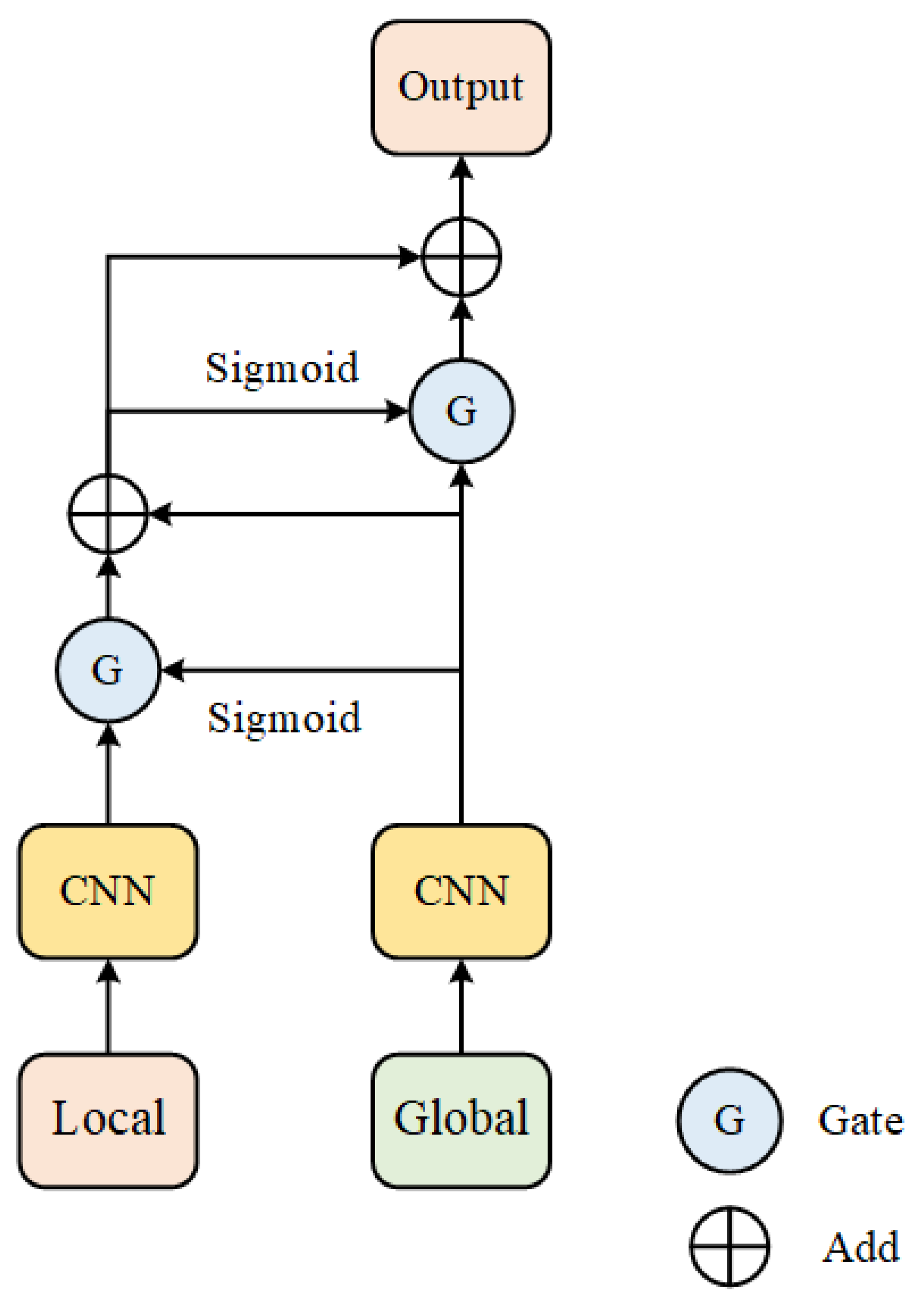
In order to filter the local and global feature and fuse them to capture the local-global context. We propose Dynamic Gatefusion (DGF) module. As shown in the Figure 3, the DGF module seems

G_{i}

and

L_{i}

i = 1, 2

as input. First, we introduce the CNN block on

G_{i}

and

L_{i}

to adjust the channel number and add linear complexity. Then we introduce the

S i g m o i d

G_{i}

to produce the first gate. Specially, the Gate is a weight between 0 and 1, which can filter the feature by dot the feature and gate. Therefore, we dot the first gate and

L_{i}

to filter the local feature. Then we add the filtered

L_{i}

and

G_{i}

and introduce

S i g m o i d

function on it to produce the second gate. And we dot the second gate and

G_{i}

to filter

G_{i}

. Then we add the filtered

G_{i}

and filtered

L_{i}

to get the local-global context. Formally, the whole process can be written as:

L_{i}^{f} = g a t e_{1} \times L_{i} + G_{i}, g a t e_{1} = s i g m o i d (G_{i})

(10)

G_{i}^{f} = g a t e_{2} \times G_{i} + L_{i}, g a t e_{2} = s i g m o i d (L_{i}^{f})

(11)

F_{l g} = L_{i}^{f} + G_{i}^{f}

(12)

where i is the stage number.

g a t e_{1}

and

g a t e_{2}

is the first gate and second gate, respectively.

s i g m o i d

is the vallian

s i g m o i d

activation function.

L_{i}^{f}

and

G_{i}^{F}

is the filtered

L_{i}

and

G_{i}

, respectively.

F_{l g}

is the local-global context.

3.2.3. DRHead

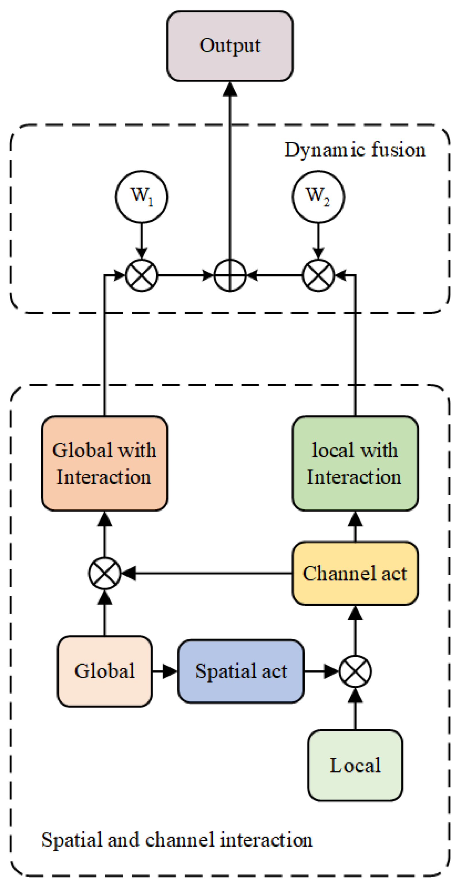
To refine the local-global context, we design a DRHead to refine the local-global context. As shown in the Figure 4, the DRHead can divided by two stage. The first stage is the spatial and channel interaction. The second stage is the dynamic fusion. The spatial and channel interaction can add the spatial and channel interaction information into the local and global feature. The dynamic fusion module can help us to dynamic fuse the local and global feature to capture the local-global context.

We seem the local and global feature as L and G, as shown in the Figure 4, we first introduce the spatial act on global feature to add the spatial interaction information into the local feature. The process can be written as:

L_{s} = S A (G) \times L

(13)

S A (.) = S i g m o i d (C o n v_{2} (R e L U (C o n v_{1} (.))))

(14)

where

S A (.)

means the spatial act,

L_{s}

means the local feature with spatial interaction information.

C o n v_{1}

and

C o n v_{2}

stand for

1 \times 1

convolution. The

C o n v_{1}

first adjust the channel number of the feature to the

C / / 16

. The

C o n v_{2}

then adjust the channel number of feature to the 1. And the

R e L U

and

S i g m o i d

is the

R e L U

and

S i g m o i d

activation function.

After we get the

L_{c}

, we conduct channel act on

L_{s}

to add the channel interaction information into the global feature G. The process can be written as:

G_{s} = C A (L_{c}) \times G

(15)

C A (.) = S i g m o i d (C o n v_{2} (R e L U 6 (C o n v_{1} (G A P (.)))))

(16)

where

C A

means the channel act,

G_{s}

stands for the global feature with spatial interaction.

G A P (.)

means the global average pooling operation. Note that we pooling the global feature to the dimension of 1 to remove the spatial information. The

C o n v_{1}

and

C o n v_{2}

stand for the

1 \times 1

conv, which adjust the channel number feature to the

C / / 16

and C, respectively. The

R e L U 6 ()

and

S i g m o i d ()

stand for the

R e L U 6

and

S i g m o i d

activation function, respectively.

After we get the

G_{s}

and

L_{c}

, we introduce a simple and effective dynamic fusion module to fuse them to capture the local-global context. As shown in the Figure 4, the

W_{1}

and

W_{2}

are two learnable parameters. The way we get

W_{1}

and

W_{2}

can be written as:

a_{1}, a_{2} = R e L U (a_{1}, a_{2})

(17)

w_{1} = \frac{a_{1}}{a_{1} + a_{2}} w_{2} = \frac{a_{2}}{a_{1} + a_{2}}

(18)

where

a_{1}

a_{2}

are two pre-defined learnable parameters.

R e L U ()

is the

R e L U

activation function. After we get

W_{1}

and

W_{2}

, we simply dot them with

G_{s}

and

L_{c}

and add them to capture the local-global context. The calucation process can be written as:

O u t p u t = W_{1} \times G_{s} + W_{2} \times L_{c}

(19)

where

W_{1}

and

W_{2}

is our learable weights,

L_{c}

and

G_{s}

stand for the local feature with channel interaction information and global feature with spatial interaction information, respectively. The

O u t p u t

means local-global context. Finally, we feed the local-global context to the segmentation head for the final prediction.

4. Experiments

4.1. Dataset

UAVid: UAVid is a fine-resolution Unmanned Aerial Vehicle (UAV) semantic segmentation dataset with two spatial resolutions (3840 2160 and 4096 2160) and eight classes. There are 420 image in total. We introduce 200 images for training, 70 images for validation and 150 images for testing. And we padded and cropped into eight 1024 × 1024 patches to train.

Vaihingen: Vaihingen consists of 33 fine-grained spatial resolution images with

2494 \times 2064

pixels. Each image has three multispectral bands (near infrared, red, green). The dataset involves five foreground classes (impervious surface, building, low vegetation, tree, car) and one background class (clutter). We introduce ID (2, 4, 6, 8, 10, 12, 14, 16, 20, 22, 24, 27, 29, 31, 33, 35, 38) for testing. And we introduce rest of images for training. The image tiles were cropped into

1024 \times 1024

px patches.

Potsdam: The Potsdam dataset contains 38 spatial TOP image tiles with size of

6000 \times 6000

pixels and the category is same as Vaihingen dataset. We introduce ID (2_13, 2_14, 3_13, 3_14, 4_13, 4_14, 4_15, 5_13, 5_14, 5_15, 6_13, 6_14, 6_15, 7_13) for testing. And we introduce the remaining 23 images for training. Same as Vaihingen, we crop the image into

1024 \times 1024

px patches in the experiments.

LoveDA: The LoveDA dataset consists of 5987 remote sensing images with

1024 \times 1024

pixels and 7 landcover categories (building, road, water, barren, forest, agriculture, and background). Specifically, we introduce 2522 images for training and 1669 images for validation. And we introduce the rest of 1796 images for testing.

4.2. Implementation Details

All of the experiments are conducted in two 3060 gpus with pytorch framework. And we introduce AdamW optimizer to train and set the learning rate to 6e-4. All of the fps are measured with the 3090 gpu.

For the UAVid dataset, we introduce random vertical flip, random horizontal flip and random brightness for data augmentation. And we set the batchsize to 8 and the epoch to 40. In the test procedure, we introduce the test-time augmentation (TTA) strategies like vertical flip and horizontal flip.

For the Vaihingen, Potsdam and LoveDA datasets, the images are randomly cropped into

512 \times 512

patches. We introduce random scale ([0.5, 0.75, 1.0, 1.25, 1.5]), random vertical flip, random horizontal flip and random rotate for training. And we set the batchsize to 16 and epoch to 100. We introduce the multi-scale and random flip for testing.

4.3. Ablation Study

4.3.1. Each Part of EDDformer

To prove the effectiveness of each part of our proposed EDDformer, we conduct the ablation study on the UAVid, Vaihingen, LoveDA, and Potsdam. For fair comparison, we remove all of the test augmentation strategy and auxiliary loss. The result are shown in Table 1.

As shown in Table 1, the baseline means we remove all of the part. And the baseline+GVformer means we only add the GVformer into the baseline model. We can see that the GVformer can add the performance largely. The mIoU increase 1.6, 0.8, 0.5, and 1.1 on UAVid, Potsdam, Vaihingen, and LoveDA, respectively. It means the global context is necessary for the remote sensing semantic segmentation and the effectiveness of the Gvformer. The baseline + DGF means we only add the DGF to fuse the feature. And we can see that it still have slight increase on four datasets, which stands for the feature filtering operation can increase the performance. We also conduct the experiment with only add the DRhead to refine the feature and we can see the performance also be increased slightly, which means the effectiveness of the DRhead and fine-grain local-global context can increase the performance.

4.3.2. GVformer

To demonstrate the effectiveness of our proposed GVformer, we replace the GVformer with different attention mechanisms. As shown in the Table 2, our GVformer achieves the best performance with the highest fps. Our Efficient Global Value Window self-attention increase the mIoU with 0.7 with Dual attention. And the parameters is lower than Dual attention (11.5 vs. 12.6). Compared with others efficient self-attention, such as Efficient multi-head self-attention and Efficient global-local attention, our methods can increase 0.1 and 2.1 in mIoU, respectively. And our the fps of our method can increase 21fps with Efficient global-local attention.

4.3.3. Backbone

In order to study the effective of the backbone, we conduct the experiment of different backbones. As shown in the Table 3. We replace the backbone with Vit-Tiny, Swin-Tiny, and CoaT-Mini. Compared with Vit-Tiny, the performance has a large decrease (68 vs. 67.1) because of the lack of the multi-scale feature. Even though the parameter of Vit-Tiny is lower than ResNet18 (8.6 vs. 11.5), the fps of Vit-Tiny decrease about 100fps. The lower FPS is not in line with the real-world application of remote sensing. And we also repalce the backbone with Swin-Tiny, the performance increase 0.6 in mIoU. But the FPS is still too low than the ResNet (63.6 vs. 136.0). Compared with CoaT-Mini, the mIoU is higher than ResNet18 with 0.5. But the FPS is still less than ResNet with 21. Therefore we choose the ResNet18 as our backbone to achieve a good trade-off.

Table 1. The Results of the each part of our proposed EDDformer, the baseline means remove all of the part.

Dataset	Method	mIoU
UAVid	baseline	66.0
	baseline+GVformer	67.6
	baseline+DGF	66.1
	baseline+DRhead	66.3
Potsdam	baseline	84.8
	baseline+GVformer	85.6
	baseline+DGF	85.0
	baseline+DRhead	84.9
Vaihingen	baseline	80.5
	baseline+GVformer	81.0
	baseline+DGF	80.7
	baseline+DRhead	80.7
LoveDA	baseline	49.2
	baseline+GVformer	50.3
	baseline+DGF	49.4
	baseline+DRhead	49.4

Table 2. The Results of different attention mechanism. And the fps is measured with the Potsdam dataset with the input of 1024 × 1024.

Attention	Complexity(G)	Parameters(M)	Speed(FPS)	mIoU
Dual attention	68.9	12.6	53.8	67.3
Efficient multi-head self-attention	67.5	12.5	63.6	67.9
Efficient global-local attention	46.9	11.7	115.6	65.9
Ours	46.4	11.5	136.0	68.0

Table 3. The Results of different backbone.

Method	Backbone	Complexity(G)	Parameters(M)	Speed(FPS)	mIoU
EDDformer	Vit-Tiny	35.31	8.6	30.2	67.1
	Swin-Tiny	104.4	12.5	63.6	68.6
	CoaT-Mini	159.7	11.7	115.6	68.5
EDDformer	ResNet18	46.4	11.5	136.0	68.0

Table 4. The inference efficiency results on the UAVid test set with others state-of-the-art methods. All of the speed evaluation are measured with 3090 gpu with input of 1024 × 1024.

Method	Backbone	Complexity(G)	Parameters(M)	Speed(FPS)	mIoU
Segmenter	Vit-Tiny	26.8	6.7	14.7	58.7
BiSeNet	ResNet18	51.8	12.9	121.9	61.5
DANet	ResNet18	39.6	12.6	189.4	60.6
ShelfNet	ResNet18	46.7	14.6	141.4	47.0
SwiftNet	ResNet18	51.6	11.8	138.7	61.1
ABCNet	ResNet18	62.9	14.0	102.2	63.8
MANet	ResNet18	51.7	12.0	75.6	62.6
SegFormer	MiT-B1	63.3	13.7	31.3	66.0
CoaT	CoaT-Mini	104.8	11.1	10.6	65.8
UNetformer	ResNet18	46.9	11.7	115.6	66.0
EDDformer	ResNet18	46.4	11.5	136.0	68.0

4.4. Comparison with State-of-the-Art Methods

4.4.1. Comparison of Inference Efficiency

For the efficient semantic segmentation of remote sensing, the parameter and fps are critical for the application. The lower parameters can reduce the memory employ of the hardware. And a high fps can expand the application scene. As shown in the Table 5, we compare our methods with others state-of-the-art methods to show that our methods can achieve a good trade-off. We can see that our methods achieve the best mIoU between these methods. Compared with the CNN-based methods, even though the FPS of BiSeNet, DANet, ShelfNet, and SwiftNet are higher than our proposed EDDformer. But our methods achieve the best mIoU and lowest parameters than these methods. Specifily, our proposed EDDformer increase BiSeNet with 61.5, which have shown the advantage of our methods and the effectiveness of our architecture. And our proposed EDDformer is higher than DANet [27] and ShelfNet by 7.4 mIoU and 21.0 mIoU. Our EDDformer also higher than SwiftNet [28] by 6.9 mIoU. The huge improvement in mIoU also prove that the effectiveness of our decoder. Compared with the transformer-based methods, our methods is higher than Segmenter by 9.3 mIoU. And our methods is higher than SegFormer and Coat by 2.0 mIoU and 2.2 mIoU. And compare with these methods, our FPS is far larger than these transformer-based methods. It proves that our method can capture the global context better and the efficient of our proposed decoder. And compared with others CNN-Transformer hybrid method, such as UNetformer, our methods still higher than UNetformer by 2.0 mIoU. And our methods is higher than UNetformer by 20.4 fps.

We list the detailed comparison result of our proposed EDDformer with others methods on the UAVid dataset. As shown in the Table 6, we can see that our methods achieve the state-of-the-art performance. Compared with the others methods, our proposed EDDformer could achieve the advantage IoU in all of the class and the best mIoU. Our proposed EDDformer outperforms the CNN-based method BiSeNet by 6.5 mIoU. And our proposed EDDformer achieves the best performance in the Clutter, Tree, StaricCar, and Human, which also prove that our proposed EDDformer has the best ability to recognition the small object.

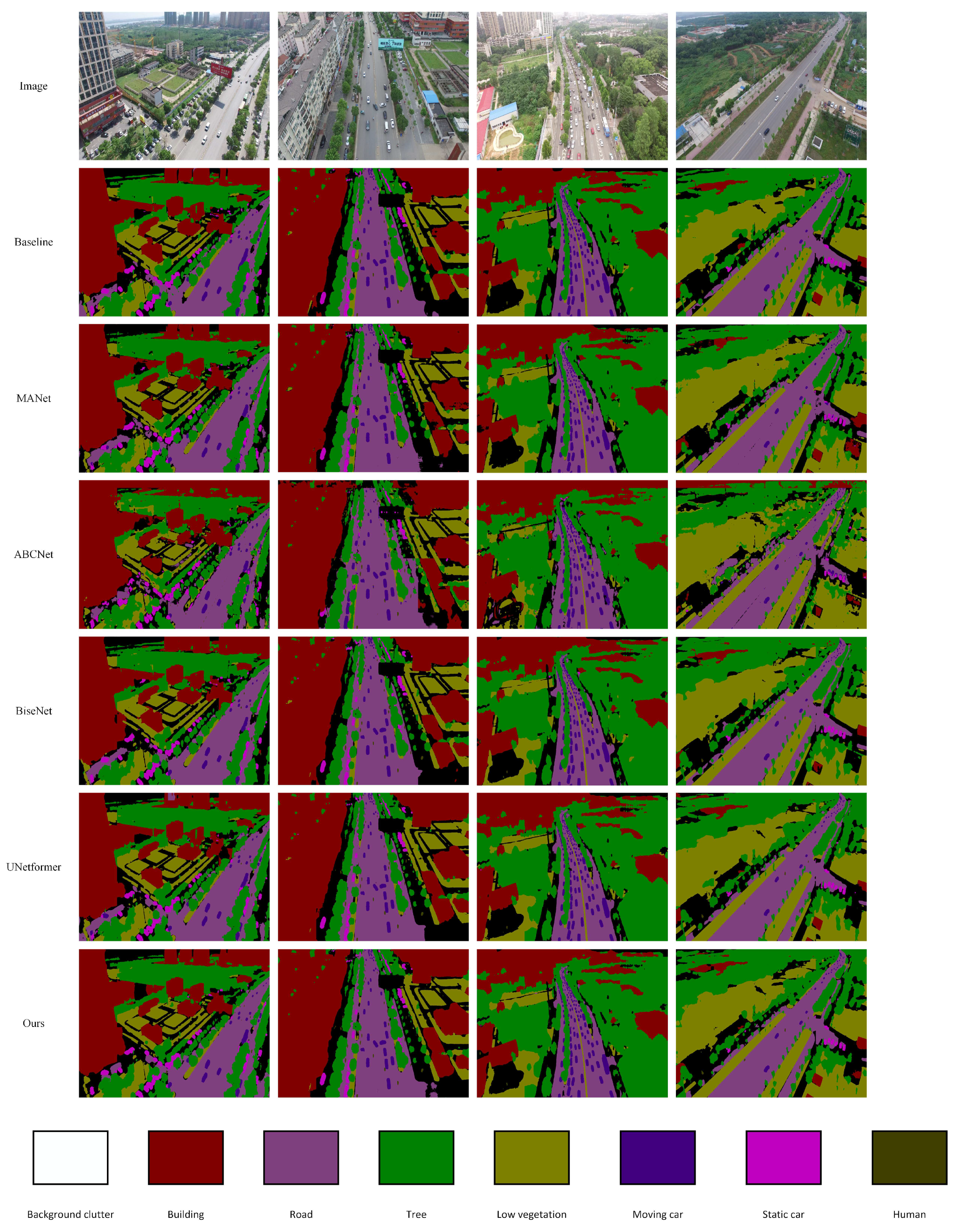
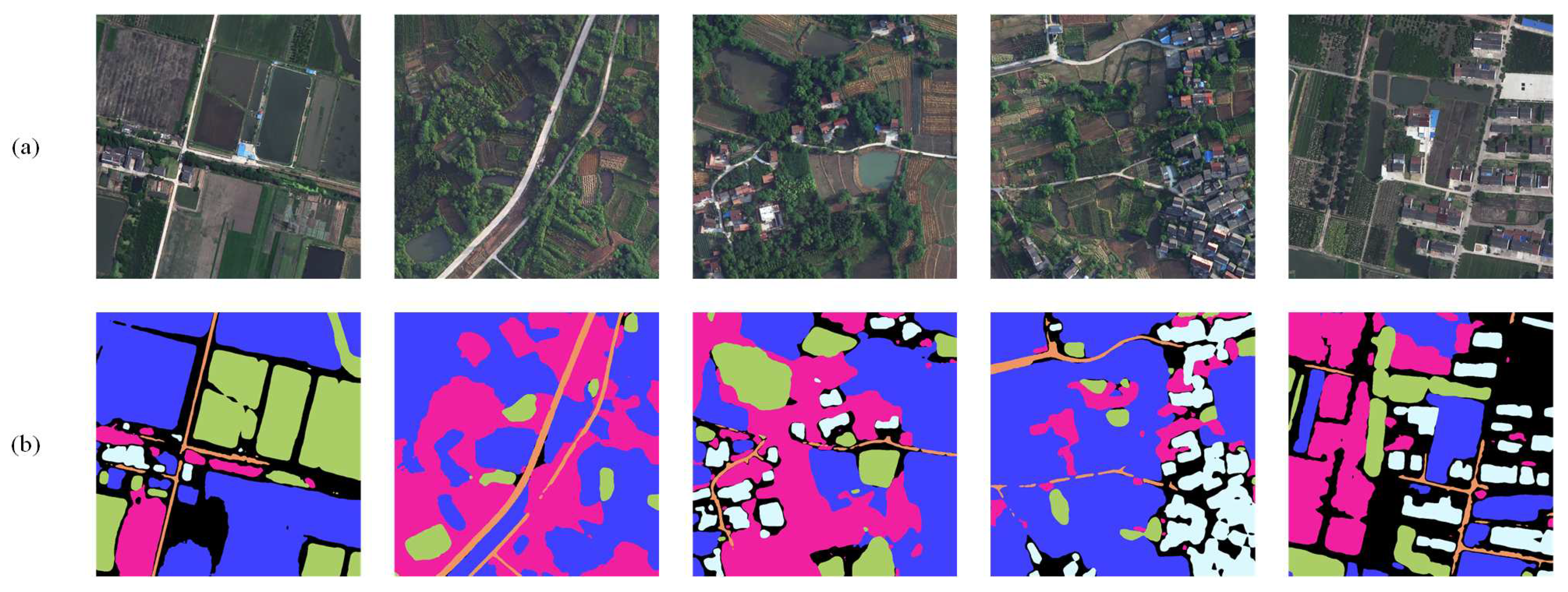
Furthermore, we compare the prediction of our method with ground-truth, Baseline, ABCNet, MANet [29], BiseNet, and UNetformer in the Figure 5.

Figure 5. The visual result of Uavid dataset.

Table 7. The detailed comparison results on the Vaihingen test set with others state-of-the-art lightweight semantic segmentation methods.

Method	Backbone	Imp.surf	Building	Lowveg.	Tree	Car	MeanF1	OA	mIoU
Segmenter	Vit-Tiny	89.8	93.0	81.2	88.5	88.5	90.4	91.0	82.7
BiSeNet	ResNet18	89.1	91.3	80.9	86.9	73.1	84.3	87.1	75.8
DANet	ResNet18	91.0	95.6	86.1	87.6	84.3	88.9	89.1	80.3
SwiftNet	ResNet18	91.8	95.9	85.7	86.8	94.5	91.0	89.3	83.8
ABCNet	ResNet18	93.5	96.9	87.9	89.1	95.8	92.7	91.3	86.5
UNetformer	ResNet18	92.9	96.4	86.6	88.1	96.1	92.0	90.5	85.5
EDDformer	ResNet18	93.6	96.9	87.9	89.1	96.5	92.8	91.4	86.8

4.4.2. Results on the Potsdam Dataset

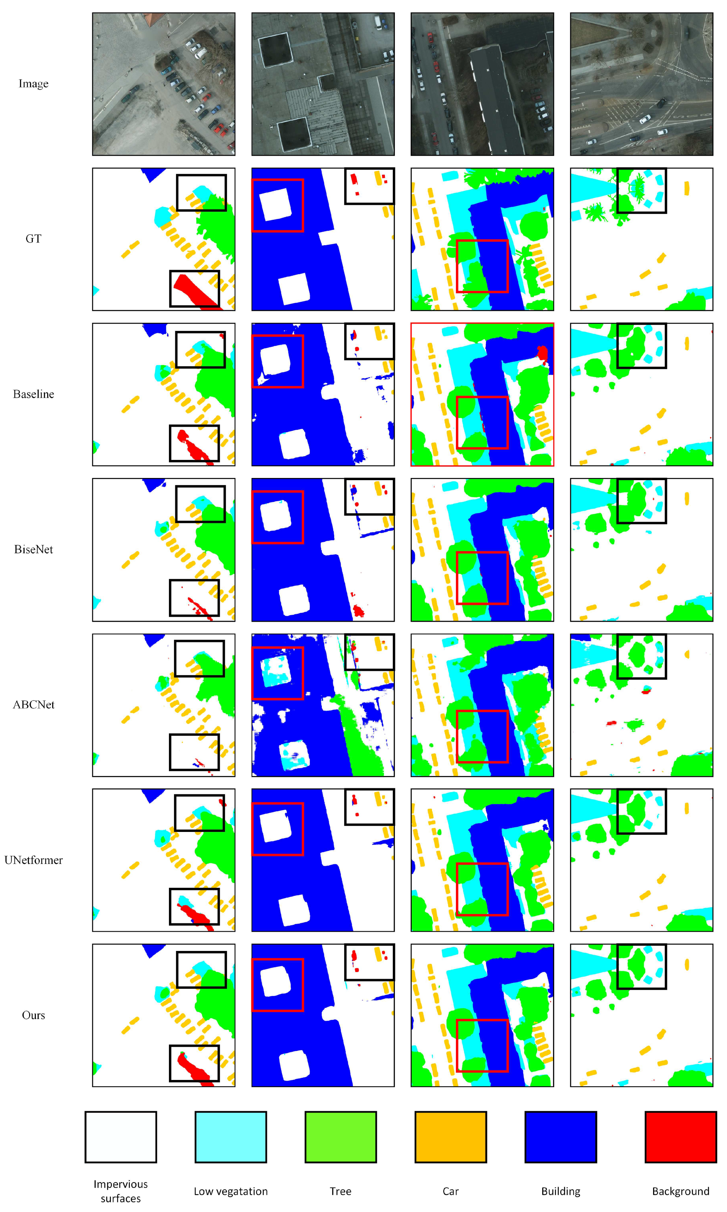
We also conduct the experiment on the Potsdam dataset. As shown in the Table, our method achieves the best mIoU, OA, and MeanF1. Compared with the Table 1 CNN based methods, our proposed EDDformer is higher than the lightweight method ABCNet and BiSeNet by 0.3 mIoU and 5.1 mIoU. And our methods is also higher than the tansformer-based method Segmenter by 6.1 mIoU. Compared with the CNN-transformer hybrid methods, our proposed is higher than the UNetformer by 1.3 mIoU, which have shown the superity of our EDDformer. Besides all, our methods achieve the best performance in every class. Furthermore, we compare the prediction of our method with ground-truth, Baseline, ABCNet, BisNet,and UNetformer. As shown in the Figure 6, in the first column, only our method can segment the Background and the Low vegetation. And in the second colume only our method can segment the impervious surface without the noise. And our method also can segment the Tree and Building in the third and fourth column.

Table 8. The detailed comparison results on the LoveDA test set with others state-of-the-art lightweight semantic segmentation methods.

Method	Backbone	Background	Building	Road	Water.	Barren	Forest	Agriculture	mIoU
Segmenter	Vit-Tiny	38.0	50.7	48.7	77.4	13.3	43.5	58.2	47.1
SemanticFPN	ResNet50	42.9	51.5	53.4	74.7	11.2	44.6	58.7	48.2
BiSeNet	ResNet18	89.1	91.3	80.9	86.9	73.1	84.3	87.1	75.8
MANet	ResNet18	91.0	95.6	86.1	87.6	84.3	88.9	89.1	80.3
ABCNet	ResNet18	93.5	96.9	87.9	89.1	95.8	92.7	91.3	86.5
UNetformer	ResNet18	49.8	57.3	61.7	87.2	15.4	38.5	36.3	49.5
EDDformer	ResNet18	45.1	57.6	56.6	79.7	17.9	45.8	62.2	52.2

4.4.3. Results on the Vaihingen Dataset

As shown in the Table, our proposed EDDformer achieves the best performance in the mIoU, MeanF1, and OA. Our EDDformer got the 86.8 mIoU, compare with the CNN-based methods, our methods is higher than the BiSeNet, ABCNet, and DANet by 11 mIoU, 0.3 mIoU, and 6.5 mIoU, respectively. And compare with the transformer-based method Segmenter, our method still higher than Segmenter by 5.1 mIoU. And our method also higher than the UNetformer by 1.3 mIoU. All of the results have shown that our EDDformer could achieve state-of-the-art performance in Vaihingen dataset. As shown in the Figure 7, we put the visual result of different methods. In the first and second column, only our method can segment the car accurate. And in the third column, our method can segment the building accurate. In the third column, only our method segment the Low vegetation witout the noise.

Figure 6. The visual result of Potsdam dataset.

Figure 7. The visual result of Vaihingen dataset.

4.4.4. Results on the LoveDA Dataset

As shown in the Table, our EDDformer can also achieve the best performance in the mIoU Compared with others methods, our proposed methods achieves 52.2 mIoU. And our EDDformer achieves the best IoU in all class. We also put the visual result of our method. As shown in the Figure 8, our method can segment the small object and building accurately.

5. Conclusion

In this paper, we proposed a new lightweight decoder-EDDformer for efficient semantic segmentation of urban remote sensing images. The decoder consists of the Efficient Global Value Transformer, Dynamic Gatefusion, and Dynamic refine head. The EDDformer can introduce the local feature once to capture local-global context. And the Efficient Global Value Transformer response for extracting the global feature. Dynamic Gatefusion can filter the local and global feature and fuse them to get the local-global context. Furthermore, the Dynamic refine head can refine the local-global context. Morever, our EDDformer can achieve the state-of-the-art performance in the Uavid, Potsdam, Vaihingen, and LoveDA with a good trade-off.

Author Contributions

Conceptualization, Bing Liu; methodology, Yansheng Gao.; formal analysis, Tongye Hu.; writing—original draft preparation, Hongwei Zhao.

Funding

This research received no external funding.

Informed Consent Statement

Not applicable.

Data Availability Statement

Publicly available datasets were analyzed in this study. This data can be found here: https://www.isprs.org/education/benchmarks/UrbanSemLab/default.aspx.

Acknowledgments

No acknowledgements.

Conflicts of Interest

The authors declare no conflict of interest.

References

Ma, Lei, et al. "Deep learning in remote sensing applications: A meta-analysis and review." ISPRS journal of photogrammetry and remote sensing 152 (2019): 166-177.
Ram, Balak, and A. S. Kolarkar. "Remote sensing application in monitoring land-use changes in arid Rajasthan." International Journal of Remote Sensing 14.17 (1993): 3191-3200.
Friedl, Mark A., et al. "Global land cover mapping from MODIS: algorithms and early results." Remote sensing of Environment 83.1-2 (2002): 287-302.
Asokan, Anju, and J. J. E. S. I. Anitha. "Change detection techniques for remote sensing applications: A survey." Earth Science Informatics 12 (2019): 143-160.
Zhao, Shaohua, et al. "An overview of satellite remote sensing technology used in China’s environmental protection." Earth Science Informatics 10 (2017): 137-148.
Xu, Yongyang, et al. "Building extraction in very high resolution remote sensing imagery using deep learning and guided filters." Remote Sensing 10.1 (2018): 144.
Ghimire, Deepak, Dayoung Kil, and Seong-heum Kim. "A survey on efficient convolutional neural networks and hardware acceleration." Electronics 11.6 (2022): 945.
Li, Xiaomeng, et al. "H-DenseUNet: hybrid densely connected UNet for liver and tumor segmentation from CT volumes." IEEE transactions on medical imaging 37.12 (2018): 2663-2674.
Yu, Changqian, et al. "Bisenet: Bilateral segmentation network for real-time semantic segmentation." Proceedings of the European conference on computer vision (ECCV). 2018.
Liu, Yuliang, et al. "Abcnet: Real-time scene text spotting with adaptive bezier-curve network." proceedings of the IEEE/CVF conference on computer vision and pattern recognition. 2020.
Strudel, Robin, et al. "Segmenter: Transformer for semantic segmentation." Proceedings of the IEEE/CVF international conference on computer vision. 2021.
Xie, Enze, et al. "SegFormer: Simple and efficient design for semantic segmentation with transformers." Advances in Neural Information Processing Systems 34 (2021): 12077-12090.
Wang, Libo, et al. "UNetFormer: A UNet-like transformer for efficient semantic segmentation of remote sensing urban scene imagery." ISPRS Journal of Photogrammetry and Remote Sensing 190 (2022): 196-214.
Wang, Junjue, et al. "LoveDA: A remote sensing land-cover dataset for domain adaptive semantic segmentation. arXiv:2110.08733 (2021).
Lyu, Ye, et al. "UAVid: A semantic segmentation dataset for UAV imagery." ISPRS journal of photogrammetry and remote sensing 165 (2020): 108-119.
Li, Haifeng, et al. "SCAttNet: Semantic segmentation network with spatial and channel attention mechanism for high-resolution remote sensing images." IEEE Geoscience and Remote Sensing Letters 18.5 (2020): 905-909.
Song, Ahram, and Yongil Kim. "Semantic segmentation of remote-sensing imagery using heterogeneous big data: International society for photogrammetry and remote sensing potsdam and cityscape datasets." ISPRS International Journal of Geo-Information 9.10 (2020): 601.
Kirillov, Alexander, et al. "Panoptic feature pyramid networks." Proceedings of the IEEE/CVF conference on computer vision and pattern recognition. 2019.
Chen, Chun-Fu Richard, Quanfu Fan, and Rameswar Panda. "Crossvit: Cross-attention multi-scale vision transformer for image classification." Proceedings of the IEEE/CVF international conference on computer vision. 2021.
Liu, Ze, et al. "Swin transformer: Hierarchical vision transformer using shifted windows." Proceedings of the IEEE/CVF international conference on computer vision. 2021.
Medsker, Larry R., and L. C. Jain. "Recurrent neural networks." Design and Applications 5.64-67 (2001): 2.
Yu, Yong, et al. "A review of recurrent neural networks: LSTM cells and network architectures." Neural computation 31.7 (2019): 1235-1270.
Fu, Rui, Zuo Zhang, and Li Li. "Using LSTM and GRU neural network methods for traffic flow prediction." 2016 31st Youth academic annual conference of Chinese association of automation (YAC). IEEE, 2016.
Pham, Huy Xuan, et al. "Gatenet: An efficient deep neural network architecture for gate perception using fish-eye camera in autonomous drone racing." 2021 IEEE/RSJ International Conference on Intelligent Robots and Systems (IROS). IEEE, 2021.
Li, Xiangtai, et al. "Gated fully fusion for semantic segmentation." Proceedings of the AAAI conference on artificial intelligence. Vol. 34. No. 07. 2020.
Rao, Yizhou, Lin He, and Jiawei Zhu. "A residual convolutional neural network for pan-shaprening." 2017 International Workshop on Remote Sensing with Intelligent Processing (RSIP). IEEE, 2017.
Zhou, Zhen, et al. "Self-attention feature fusion network for semantic segmentation." Neurocomputing 453 (2021): 50-59.
Orsic, Marin, et al. "In defense of pre-trained imagenet architectures for real-time semantic segmentation of road-driving images." Proceedings of the IEEE/CVF Conference on Computer Vision and Pattern Recognition. 2019.
Chen, Bingyu, et al. "MANet: A multi-level aggregation network for semantic segmentation of high-resolution remote sensing images." International Journal of Remote Sensing 43.15-16 (2022): 5874-5894.
Chen, Chun-Fu Richard, Quanfu Fan, and Rameswar Panda. "Crossvit: Cross-attention multi-scale vision transformer for image classification." Proceedings of the IEEE/CVF international conference on computer vision. 2021.

Figure 2. (a) Efficient Global Value Transformer, (b) Efficient Global Value Window self-attention, (c) Channel path, (d) Spatial path.

Figure 3. The design of dynamic gatefusion module.

Figure 4. The design of DRHead.

Figure 8. The visual result of loveda dataset. (a) is the original image, (b) is the segment of our map.

Table 5. The detailed comparison results on the UAVid test set with others state-of-the-art lightweight semantic segmentation methods.

Method	Backbone	Clutter	Building	Road	Tree	Vegetation	MovingCar	StaticCar	Human	mIoU
Segmenter	Vit-Tiny	64.2	84.4	79.8	76.1	57.6	59.2	34.5	14.2	58.7
BiSeNet	ResNet18	64.7	85.7	61.1	78.3	77.3	48.6	63.4	17.5	61.5
DANet	ResNet18	64.9	85.9	77.9	78.3	61.5	59.6	47.4	9.1	60.6
SwiftNet	ResNet18	64.1	85.3	61.5	78.3	76.4	51.1	62.1	15.7	61.1
ABCNet	ResNet18	67.4	86.4	81.2	79.9	63.1	69.8	48.4	13.9	63.8
MANet	ResNet18	64.5	85.4	77.8	77.0	60.3	67.2	53.6	14.9	62.6
SegFormer	MiT-B1	66.6	86.3	80.1	79.6	62.3	72.5	52.5	28.5	66.0
CoaT	CoaT-Mini	69.0	88.5	80.0	79.3	62.0	70.0	59.1	28.9	65.8
UNetformer	ResNet18	66.0	86.5	80.1	79.5	63.3	55.3	67.6	29.0	66.0
EDDformer	ResNet18	67.0	86.8	80.4	79.7	63.2	63.1	73.0	30.6	68.0

Table 6. The detailed comparison results on the Potsdam test set with others state-of-the-art lightweight semantic segmentation methods.

Method	Backbone	Imp.surf	Building	Lowveg.	Tree	Car	MeanF1	OA	mIoU
Segmenter	Vit-Tiny	91.5	95.3	85.4	85.0	88.5	89.2	88.7	80.7
BiSeNet	ResNet18	89.1	91.3	80.9	86.9	73.1	84.3	87.1	75.8
DANet	ResNet18	90.0	93.9	82.2	87.3	44.5	79.6	88.2	69.4
SwiftNet	ResNet18	92.2	94.8	84.1	89.3	81.2	88.3	90.2	79.6
ABCNet	ResNet18	92.7	95.2	84.5	89.7	85.3	89.5	90.7	81.3
UNetformer	ResNet18	92.9	95.2	85.0	90.7	88.2	90.4	91.1	82.7
EDDformer	ResNet18	93.1	95.8	85.3	90.9	89.5	90.9	91.4	83.5

Disclaimer/Publisher’s Note: The statements, opinions and data contained in all publications are solely those of the individual author(s) and contributor(s) and not of MDPI and/or the editor(s). MDPI and/or the editor(s) disclaim responsibility for any injury to people or property resulting from any ideas, methods, instructions or products referred to in the content.

© 2023 by the authors. Licensee MDPI, Basel, Switzerland. This article is an open access article distributed under the terms and conditions of the Creative Commons Attribution (CC BY) license (http://creativecommons.org/licenses/by/4.0/).

Copyright: This open access article is published under a Creative Commons CC BY 4.0 license, which permit the free download, distribution, and reuse, provided that the author and preprint are cited in any reuse.

MDPI Initiatives

Important Links

Choose an area of interest and we will send you notifications of new preprints at your preferred frequency.

Disclaimer

EDDformer: A New Decoder for Efficient Semantic Segmentation of Remote Sensing Urban Scene Imagery

Abstract

1. Introduction

2. Related Work

3. Methods

3.1. Encoder

3.2. Decoder

3.2.1. Efficient Global Value Transformer

3.2.2. Dynamic Gatefusion Module

3.2.3. DRHead

4. Experiments

4.1. Dataset

4.2. Implementation Details

4.3. Ablation Study

4.3.1. Each Part of EDDformer

4.3.2. GVformer

4.3.3. Backbone

4.4. Comparison with State-of-the-Art Methods

4.4.1. Comparison of Inference Efficiency

4.4.2. Results on the Potsdam Dataset

4.4.3. Results on the Vaihingen Dataset

4.4.4. Results on the LoveDA Dataset

5. Conclusion

Author Contributions

Funding

Informed Consent Statement

Data Availability Statement

Acknowledgments

Conflicts of Interest

References

MDPI Initiatives

Important Links

Subscribe