Adaptive Terrain Perception and Decision-Making Systems for Agile Mobile Robots in Dynamic Search and Rescue Scenarios

Beginning with navigation system design, this paper presents a comprehensive strategy for enhancing the search and rescue capabilities of agile mobile robots. Towards this, the autonomous ground vehicle (AGV) utilizes surface classification to determine and prioritize the terrain it is traversing. Our developed system design incorporates real-time terrain data with task objectives at a high level, ensuring that the robot can effectively navigate complex and ever-changing environments. This design, in conjunction with the introduction of a novel lightweight surface classification model, forms the basis of our adaptive terrain perception and decision-making systems, enabling robots such as Jackal to adapt rapidly and make the decisions necessary to complete the task. Subsequently, we exhaustively validated these systems through a series of extensive experiments in a variety of terrains, including normal and mixed terrains, demonstrating their robustness and efficacy in real-life situations.

Keywords:

Subject: Engineering - Other

1. Introduction

Across industries such as manufacturing, logistics, and healthcare, the use of mobile robotics for tasks spanning from product transportation and facility inspection to patient assistance has increased significantly. Despite the fact that these robots are designed for autonomous navigation, their ability to traverse a variety of terrains efficiently is crucial to their overall performance [1,2,3]. Terrain surface classification methods for autonomous ground vehicles (AGVs) have seen significant advancements in recent years [4,5,6,7]. Identifying the type of terrain, a complex aspect of environmental perception, has a significant impact on both the motion [8] planning and the control [9] of mobile robotics. Due to their robust propulsion systems, mechanical dependability, and environmental adaptability, tracked mobile robots are commonly used for hazardous duties such as cartography [10], search missions [11], and mining operations [12]. When navigating complex surfaces, the ability of these robots to surmount obstacles depends primarily on the interaction between their treads and the ground. In order to efficiently manage energy and to enable intelligent supervision of the robot, it is essential to accurately recognize the various terrain types.

There are two main ways to identify the type of ground a robot is moving over: active and passive methods [7,13]. Active methods use external sensors like cameras and radars to look at the ground, but this can be unreliable and computationally heavy, so often a combination of sensors is used, which can be expensive and complex [14]. These sensors can also be affected by weather conditions, like light and humidity [15]. On the other hand, passive methods use internal sensors that feel the robot’s movements and feedback, such as accelerometers and gyroscopes, to understand the terrain [16]. This is simpler and doesn’t need extra equipment. An easy-to-collect internal signal, the driving current signal from the motor controller [17], is also very useful for this purpose [15]. However, most studies in this field have mainly focused on situations where the robot is moving at a single speed in a straight line, which is not always practical for real-time tasks [18]. Therefore, terrain surface classification emerges as a crucial instrument for enabling mobile robots to navigate these diverse terrains by precisely identifying and categorizing surface types, thereby enabling precise control actions [19]. This vital data enables robotics to make intelligent judgments regarding optimal routes, pace adjustments, and traction optimization. In dynamic search-and-rescue scenarios where time is of the essence, the rapid and efficient navigation of mobile robotics through unpredictably rugged terrain is of the uttermost importance [20].

Researchers use theories about how tracks interact with soil to develop mathematical solutions to identify the type of terrain [21,22]. But, understanding the detailed interactions between tracks and soil is very complicated and requires a lot of computer power. Many researchers use machine learning (a type of computer learning) to effectively identify terrains. There are two main types of machine learning: supervised and unsupervised [23]. Methods such as the support vector machine and random forest classifier are examples of supervised learning approaches that have proven successful in identifying terrains compared to unsupervised methods [19,24]. However, the effectiveness of traditional machine learning methods that rely on learning features is not sufficient when dealing with complex situations [25]. Some researchers also use different kinds of neural networks, which are computer models designed to think like humans, like probabilistic neural network or backpropagation [26], for identifying terrains. When these are combined with unsupervised learning, like deep belief network, they can better learn and understand terrains.

In the field of autonomous ground vehicle-based classification, the integration of deep learning techniques has significantly enhanced our capacity to comprehend and categorize diverse terrain types. A notable approach, known as "EfferDeepNet" [27], as elucidated in the paper titled "EfferDeepNet: An Efficient Semantic Segmentation Method for Outdoor Terrain," amalgamates the strengths of two formidable networks, EfficientNet and DeepLabV3+. This amalgamation yields a robust model adept at swiftly and accurately discerning distinct terrain features. Additionally, Mei et al. [28] introduce the "1DCL" method, which empowers robots to interpret terrain attributes by analyzing vibrations. Consequently, the limitations imposed by constrained computing resources and energy budgets in embedded platforms underscore the necessity of making meticulous trade-offs between model complexity and efficiency.

Addressing the challenge posed by restricted computing resources, research has given rise to specialized lightweight deep learning architectures. These architectures offer initial solutions to facilitate efficient deployment within these constraints. A prominent illustration of this is evident in the MobileNet series, exemplified by MobileNetV1 [29]. This series introduces depthwise separable convolutions, effectively reducing computational overhead and paring down the model’s parameter count, all while preserving accuracy. MobileNetV2 [30] builds upon this foundation by incorporating innovations like inverted residual blocks, achieving remarkable efficiency with a modest parameter count of just 2.3 million. The latest iteration, MobileNetV3 [31], pushes the boundaries of efficiency even further by harnessing automated architecture search, requiring a mere 1.5 million parameters. Beyond the MobileNet series, alternative architectures like SqueezeNet [32] adopt 1x1 pointwise filters to reduce model dimensions, while ShuffleNet [33] optimizes computational efficiency through group convolutions and channel shuffling. Moreover, EfficientNet [34] embraces a holistic scaling approach, meticulously harmonizing network dimensions, resulting in models that are both resource-efficient and potent. This collective endeavor drives forward the field of efficient deep learning for embedded devices.

This article centers on the development of lightweight terrain surface classification models, employing interoceptive sensors to establish a versatile terrain identification system for mobile robots. The significant contributions are as follows:

We introduce a novel classifier framework that integrates path planning into complex tasks such as search and rescue missions for mobile robots.To tackle the classification task, we leverage a Fourier gating mechanism-driven atrous Convolutional Neural Network (CNN) known as TerraWave, specifically designed for terrain surface classification.
For path planning algorithms, we utilize a graph connectivity method to search for the most efficient route from the starting state to the target or goal state.
We present a comprehensive structure for analysis, where the classifier collaborates with graph-based path planning to find the optimal solution, supported by a local classifier detector.

2. System Overview

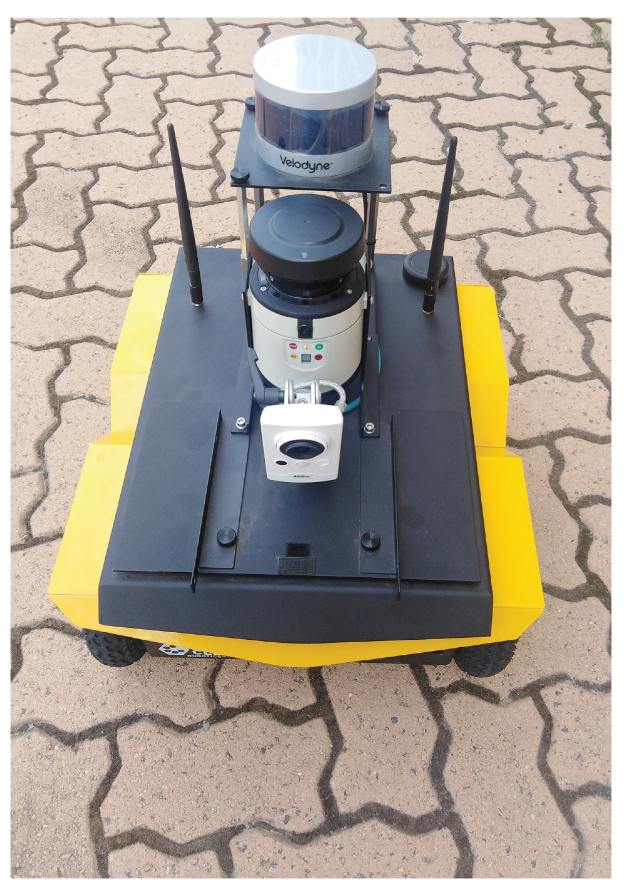
Jackal is a small, fast, entry-level field robotics research platform, which has an onboard computer, GPS and IMU fully integrated with ROS for out-of-the-box autonomous capability. It has a maximum speed of 2.0

m / s e c

with a maximum payload of 20

k g

. Figure 1 shows LMS 111 equipped Jackal AGV in the Autonomous system lab of UNSW Canberra.

Jackal is a skid-steer mobile robot (SSMR), driven by four wheels. It has two DC electric motors and each motor drives two wheels on each side. These two wheels are linked via a chain on sprocket drive and gearing where the left and right side drive assemblies are identical. The two wheels on each side of the jackal are driven independently and the vehicle’s rotation is achieved by driving left and right side wheels at different velocities. In order to move the vehicle straight, the velocities of the left and right side wheels should be the same [35].

Ground vehicle platform: JACKAL as AGV.
Processor: Intel i5-4570TE Dual Core, 2.7 GHz Processor with 8GB RAM.
Sensors: RGB Camera, in-built Odometer fused with IMU.
OS: ROS Kinetic Kame in Ubuntu 16.04.

Table 1. Jackal Dimensions.

Jackal Parts	Value	Unit
Chassis Length	420	mm
Chassis Width	310	mm
Chassis Height	184	mm
Wheel Radius	98	mm
Wheel Width	40	mm
Wheel Base	262	mm
Track Width	375.6	mm

2.1. RGB Camera

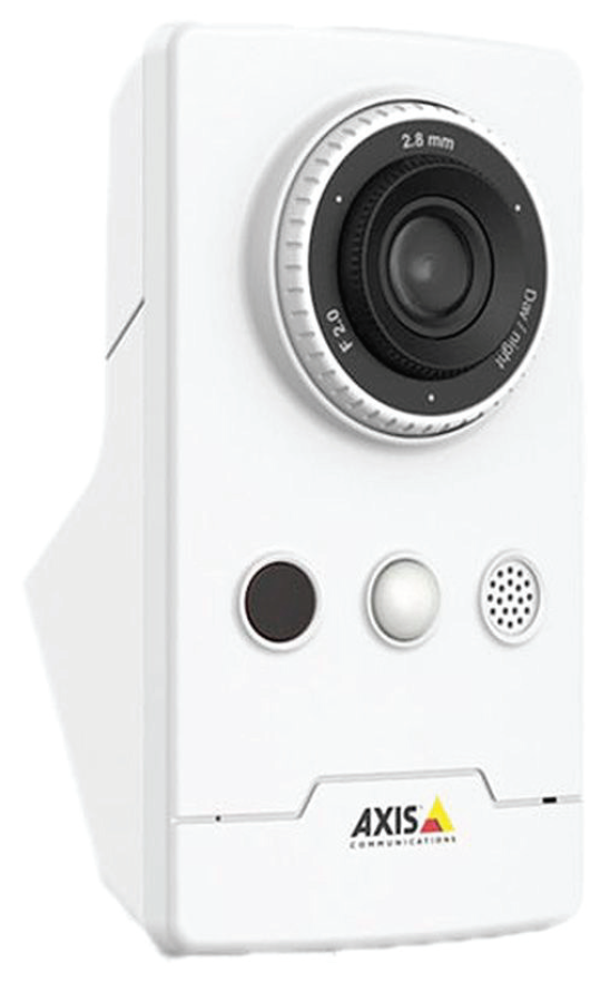
AXIS Companion Cube L [Figure 2] features high-quality video in HDTV 1080p / 2 MP resolution and also offers IR illumination and day and night functionality.

The axis camera data is only used to identify the ground surfaces and the image frame is split-ted vertically into two parts. Then these divided image frames are fed into the

Q_{β}

classifier model. The model gives an output surface score as well as image location in a particular scene. The surface score decides the AGV’s path depending on the controller’s effort.

Table 2. Axis Camera Specification.

Features	Values
Image sensor	1/3 scan RGB CMOS
Frame rate	25/30 fps
Horizontal FoV	110 $^{\circ}$
Vertical FoV	61 $^{\circ}$
Fixed focal length	2.8 mm, F2.0

2.2. ROS Framework

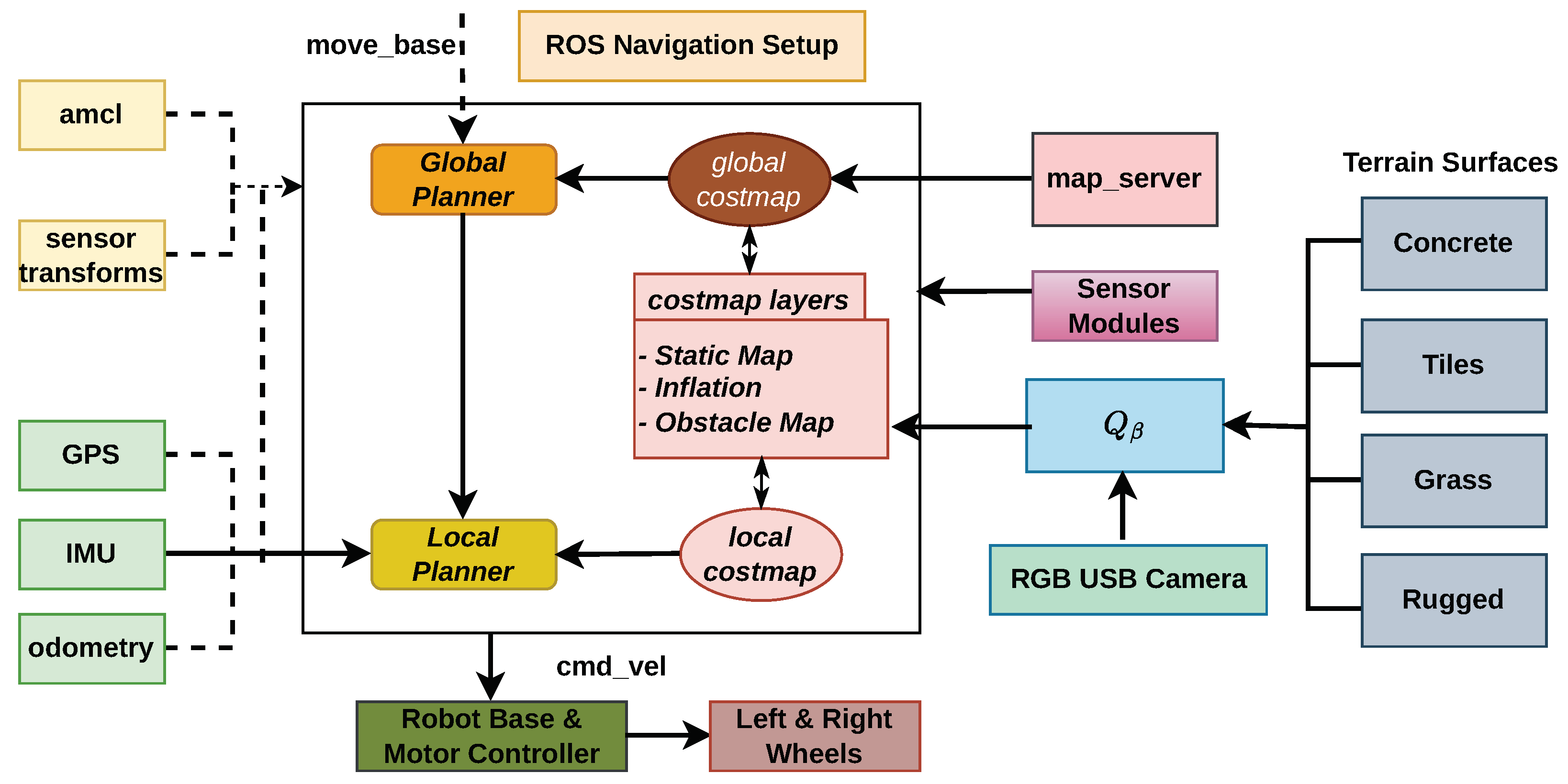
The ROS navigation module heavily relies on the Layered costmap “

c o s t m a p_2 d

" ROS package, which is obtained by sensors and transforms the map data into a format that the path planner can easily understand. It creates a map of the robot’s surroundings, including any obstacles and freely accessible areas, using sensor data. Each location on the map is given a cost value by the costmap, which represents how difficult it is for the robot to navigate through the area. This information can be utilized by the robot to plan its path to prevent obstacles [36].

In general, there are two types of costmap representation in the navigation module: the global and local costmap. The global costmap is produced using the global sensor data obtained from the robot’s vision sensor and LiDAR, and it is utilized for global planning. The robot’s local sensor data, such as that from its ultrasonic or infrared sensors, are utilized to build the local costmap, which is used for short-term planning.

The master costmap layer incorporates a static map layer, an obstacle map layer and an inflation layer. The static map layer depicts a section of the cost map that is mainly static, similar to those produced by SLAM. Throughout the robot’s operation, the static layer represents the environment’s stationary obstacles, such as walls and furniture. An obstacle layer uses data from lidar, depth cameras, etc. to locate any solid, potentially moving objects that are nearby. For the costmap to accurately represent the robot’s configuration space, the inflation layer adds additional values around lethal barriers (i.e., inflates the obstacles).

For Costmap ROS navigation to operate effectively, the environment is divided into a grid of cells. Based on the sensor data, a cost value is assigned to each cell. Each grid has a value between 0 and 254; larger values indicate a greater danger of entering the area, which suggests that the grid is blocked by an obstacle. With the cost value 0 denoting free space, and as a result, the robot shouldn’t be prevented from traveling there. The cell value 255 is allocated for blank cells; additionally, the values 254 and 253 are set aside for obstacles and inscribed (inflation), respectively.

The proposed framework inserts the cost value into the costmap for the area where the image score which is generated by the surface classifier is more. So, the robot will avoid this particular region independent of any obstacles.

3. TerraWave Classifier

The TerraWave classifier (

Q_{β}

) utilizes an Atrous convolution structure coupled with a channel-wise Fourier gating mechanism(FGM) to extract prominent features through dilated CNNs. Therefore, Atrous convolution [37], also termed as dilated convolution, involves the use of filters of varying sizes, known as pyramid dilated convolutions. The concept is to design a lightweight model based on the FGM to reduce the number of parameters and improve computational performance for custom terrain datasets. To attain broader line features, we introduce spaces into the regular filter map, widening the covered area without adding more details or increasing depth. This method enables the capture of broader feature information.

When considering 2-D atrous convolution with a dilation rate d in the range

[1, N_{d}]

, it can be expressed as:

\begin{matrix} c [i, j] & = \sum_{d = 1}^{N_{d}} (\sum_{k = 1}^{M} \sum_{l = 1}^{N} x [i + d k, j + d l] \cdot W_{c} [k, l]) + b_{c} \end{matrix}

(1)

Here, d is the dilation rate, k and l are the kernel indices, and

d k

and

d l

represent the effective stride in the height and width dimensions, respectively, due to the dilation.

c [i, j]

denotes the output value at location

(i, j)

for simplicity. The input at the dilated location is defined as

x [i + d \cdot k, j + d \cdot l]

with the convolutional kernel weight of

W_{c} [k, l]

and

b_{c}

as the bias term.

The Fourier Transform [38,39] gating operation can be represented as:

X_{fft} [i, j, u, v] = \sum_{i = 0}^{H - 1} \sum_{j = 0}^{W - 1} c [i, j] \cdot e^{- j 2 π (\frac{u i}{H} + \frac{v j}{W})}

(2)

where:

X_{fft} [i, j, u, v]

represents the Fourier Transformed input, and u and v are the frequency indices in the height and width dimensions, respectively.

The FGM is applied as:

X_{fft, gated} [i, j, u, v] = g [u, v] \cdot X_{fft} [i, j, u, v]

(3)

where

g [u, v]

is the learned gating parameter for frequency components u and v.

Finally, the Inverse Fourier Transform is applied to return to the spatial domain:

x_{ifft} [i, j] = F^{- 1} {X_{fft, gated} [i, j, u, v]}_{u, v = 0}^{H - 1, W - 1} = \frac{1}{H W} \sum_{u = 0}^{H - 1} \sum_{v = 0}^{W - 1} X_{fft, gated} [i, j, u, v] \cdot e^{j 2 π (\frac{u}{H} + \frac{v}{W})}

(4)

The output of the FGM is the real part of the Inverse Fourier Transformed and gated tensor:

C_{out} [i, j] = Real {x_{ifft} [i, j]}

(5)

4. Grid-based Path-Planning Approach

To implement the effective path panning algorithm in ROS, a number of packages, including

c o s t m a p_2 d

g l o b a l_p l a n n e r

, and

l o c a l_p l a n n e r

, has be used. The occupancy grid map, a representation of the robot’s surroundings, is produced and updated by the

c o s t m a p_{2} d

package. The

g l o b a l_p l a n n e r

determines a route from the robot’s current location to its goal while accounting for potential hazards and the dynamic restrictions of the robot. On the other hand, the

l o c a l_p l a n n e r

creates a trajectory that advances the robot toward its objective while adhering to the global planner’s suggested course. The algorithm divides the environment into equal-sized cells and assigns values to each cell based on the obstacles encountered, resulting in a discrete grid map of the environment. A variety of search techniques can be utilized to effectively plan paths using the grid map structure. Finding a collision-free path between the start and end points while taking into account all potential hazards is known as global path planning. Local path planning, in contrast, creates a smooth and obstacle-free trajectory from the current position to the objective position by just taking into account the robot’s immediate surroundings. Grid-based path planning is computationally effective, scalable, and capable of navigating through challenging landscapes that contain obstacles of all different sizes and shapes.

Within its operational environment, local path planning involves selecting a path automatically for the robot to proceed from its current position to either the objective position or the next position. On the other hand, global path planning is concerned with choosing the best route through the environment from the robot’s starting location to its end destination. For a robot to navigate safely and without colliding with anything, both local and global path planning must cooperate. Robots can move safely and effectively through cluttered and dynamic settings due to the effective integration of these two path planners. Grid-based local and global path planning will continue to be essential to the development of robotic technology considering the promising advancements in ROS and path planning algorithms.

4.1. Local Planner

A more precise depiction of the environment is made possible by the use of gridmaps and cost functions, enabling the robot to travel through confined locations and avoid obstacles more successfully. For smooth and secure navigation, local motion planning algorithms are crucial in robotic applications. One such technique is the dynamic window approach (DWA), which is based on the idea of a robot’s dynamic window, which is the collection of achievable velocities while avoiding impediments. The method determines the robot’s future positions by computing the change in speed and heading angle.

4.2. Global Planner

It entails planning a path for the robot to traverse from its current location to its destination while accounting for terrain, barriers, and other factors. The goal of global path planning is to make sure the robot moves through the environment quickly, safely, and without running into any obstacles. A modified D* light algorithm is used to complete the task. A single costmap created by the ROS navigation stack serves as a starting point for path planning and obstacle avoidance. For instance, the static layer represents objects like walls and buildings that remain the same over time. The robot footprint layer also shows the area the robot occupies, which is important to know so it can move without crashing into any object.

4.3. Obstacle and Inflation Layer

One of the crucial layers in the Costmap navigation system is the inflation layer. This layer avoids the robot from colliding with static obstacles by forming a buffer around them. Each cell in the buffer zone is given a cost value, which rises as the distance to the obstacle decreases, enabling collision avoidance. The inflating layer ensures that the robot’s travel path is safe and sufficiently far from the static barriers. By giving the robot the space it needs to safely traverse between obstacles, inflated costmaps will be utilized to discern between traversable space and obstacles in the surroundings. Setting up this layer properly involves altering the parameters that govern the robot’s motion in the surroundings to move as efficiently as possible.

The parameters tuned for the Navigation packages are listed in the Tables below.

Table 3. Costmap Common Parameters.

Parameters	Values
Obstacle_range	2.0
raytrace_range	2.5
obstacle_layer	enabled
inflater_layer	enabled
inflation_radius	0.20
inflation_radius	0.20

Table 4. MOVE_BASE Parameters.

Parameters	Values
controller_frequency	5.0
controller_patience	10.0
planner_frequency	2.5

Table 5. GLOBAL_COSTMAP Parameters.

Parameters	Values
global_frame	map
robot_base_frame	base_link
update_frequency	5.0
publish_frequency	5.0
plugins(layers)	static, Obstacle, inflater
static_map	true

Table 6. LOCAL_COSTMAP Parameters.

Parameters	Values
global_frame	map
robot_base_frame	base_link
update_frequency	5.0
publish_frequency	2.0
rolling_window	true
static_map	false

Table 7. Robot Configuration Parameters.

Parameters	Values
max_vel_x	1.0
min_vel_x	0.0
acc_lim_x	1.0
acc_lim_theta	2.0
octdist_scale	0.4
dwa	true
max_vel_theta	1.57
min_vel_theta	-1.57
holonomic_robot	false
escape_vel	-0.5

5. Framework

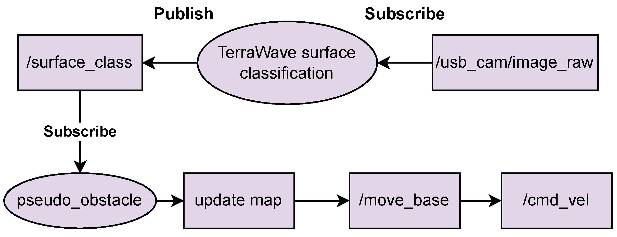
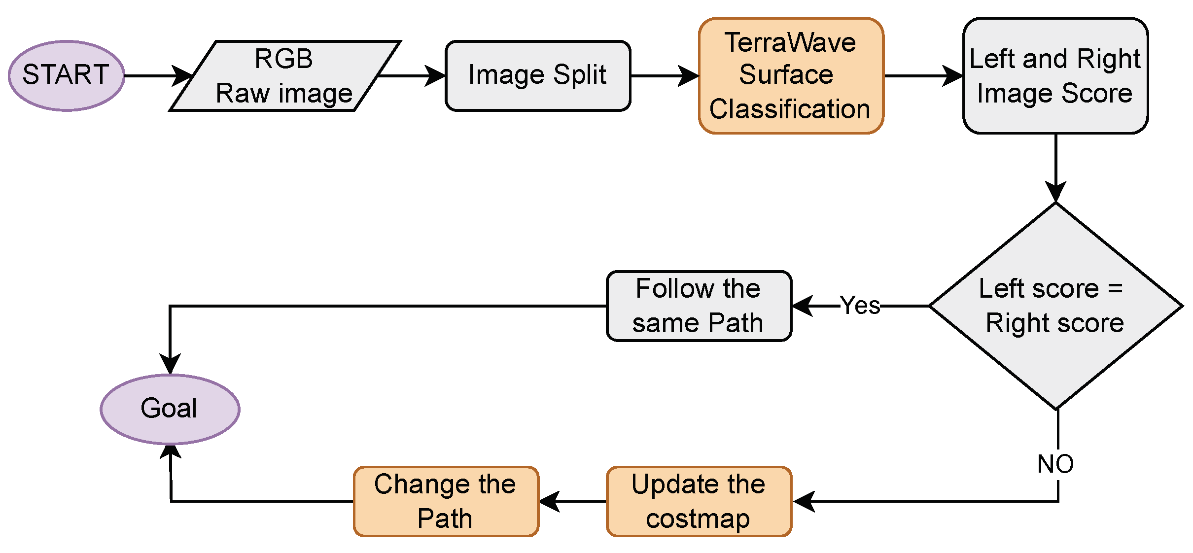
The RGB camera is mounted on the Jackal. The trained TerraWave is implemented as a ROS node along with the navigation package. Initially CNN model node with subscribe the Raw images from the usb camera node. Then the images are split vertically along the center into left and right frames. It classifies the surface into four categories and publishes image scores. If the image scores are equal, there is no change in the cost value of the costmap. Rather image scores are different, the cost values in the inflation layer are inserted into the high image score region. The inflation layer is updated periodically along with the obstacle and static layer. It will update the cost values to the master cost map of entire map. Later, path planner module will replan the path so that the robot will avoid the terrain region with high image score. The process will continue until the robot reaches its defined goal. The flowchart of the proposed framework is illustrated in Figure 5

Figure 4. ROS Surface Classification Package Node.

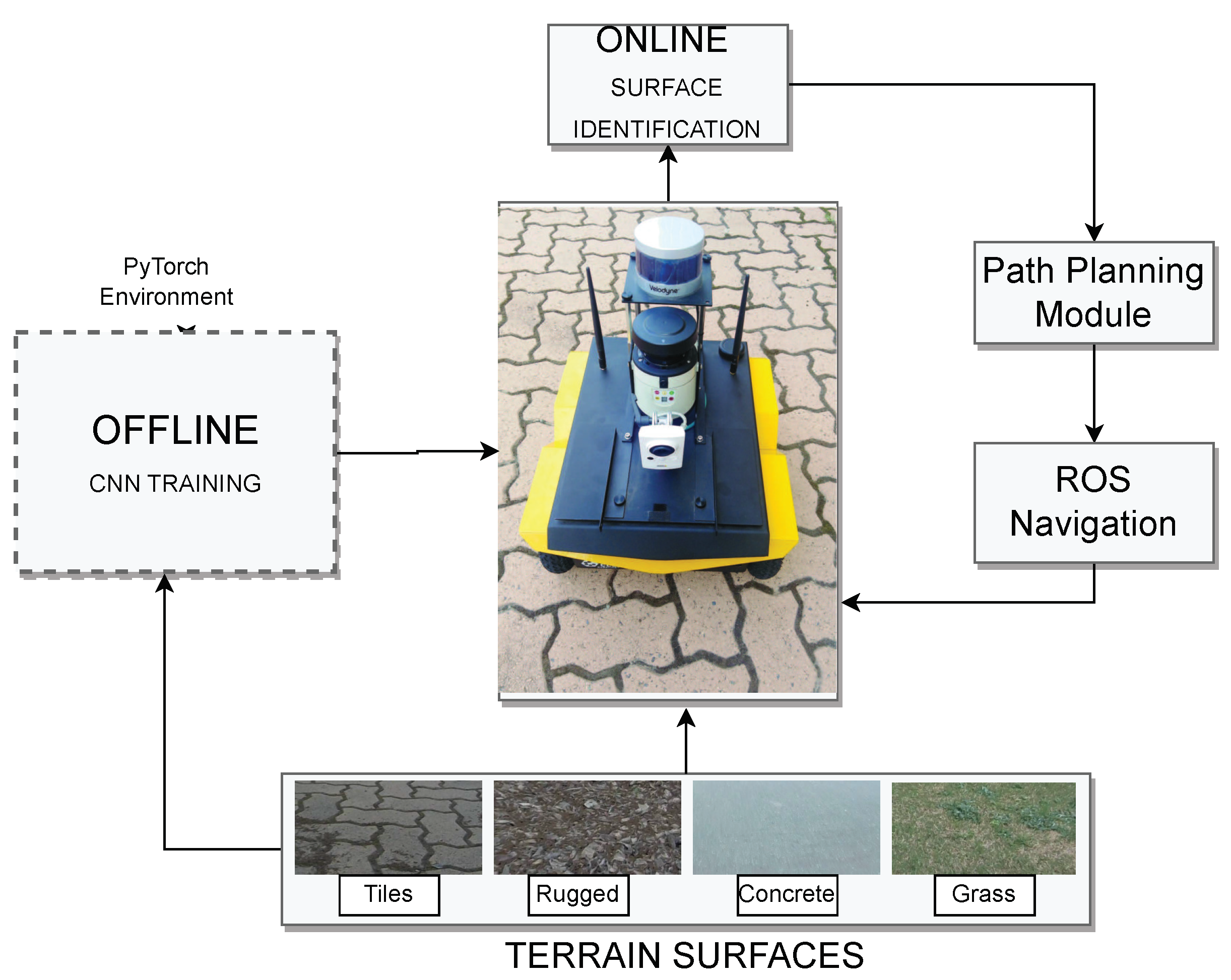
Figure 5. Software Framework.

Figure 6. Framework of surface Classification.

6. Path-Planning Notations

A path is essentially defined as a collection of waypoints, goals, states, cells, nodes, or vertices defined in (x, y) coordinate systems in metric-based path planning. The entire planning area is discretized into non-overlapping grid cells that represent the graph as subsets of the configuration space, also known as C-space. A connectivity graph illustrates how adjacent cells are connected for traversing, and the search space is divided into a finite number of states the AGV can traverse. These states’ characteristics, such as the positions and orientations of vehicles, are described for the environment’s state space. As a result, a graph search algorithm searches the state space for a set of cells that define a route from the starting state to the target or goal state.

In path planning [40], a configuration space

C

ℜ^{N}

is represented by the vector of joint variables, S, where

N

indicates whether the world dimension is 2D or 3D; in this work, (

N

=2). The workspace,

W

{

A

(q)

⊂

W

}, that an AGV occupies in the grid map is represented by

A

(q)

, while A represents the geometry of an AGV. The configuration space’s workspace,

W

ℜ^{2}

, has three dimensions (x, y, and

θ

) and is filled with obstacles. The x and y variables, which indicate the position in the 2D space, entirely specify the AGV’s position in that dimension. The obstacle region in the workspace is indicated by the notation

O_{o b s}

⊂

W

, while the obstacle region in the configuration space,

C_{o b s}

, is designated as

C_{o b s} = {q \in C | A (q) \cap O_{o b s} \neq \emptyset}

(6)

The free space (

C_{f r e e}

C

C_{o b s}

) is the collection of configurations that prevent collisions. The purpose of the path-planning issue is to determine a route across the configuration space from an initial point (

S_{s t a r t}

) to a specific destination position (

S_{g o a l}

) so that the AGV does not run into any obstacles. In the literature on path planning, a collision-free path from the starting point to the destination is shown as a continuous map,

Q

, as

\begin{matrix} C : [s t a r t, g o a l] \Rightarrow Q_{c o l l i s i o n f r e e p a t h} \end{matrix}

(7)

\begin{matrix} C (s t a r t) = S_{s t a r t} : C (g o a l) = S_{g o a l} \end{matrix}

(8)

with

O_{o b s}

primarily detected by the vision sensor. The trajectories of the dynamic obstacles are stated as a function of time with T⊂ℜ signifying the time interval and a state

X

defined as

X

C

×T as we examine both static and dynamic obstacles in our workspace.

X_{o b s} = {(q, t) \in X | A (q) \cap O_{o b s} (t) \neq \emptyset}

(9)

describes the dynamic obstacle regions in X, where

O_{o b s}

(t) denotes a time-varying obstacle. By isolating the path-planning method into a collision-free path with a time function, it is modified for

X

7. Results and Discussion

7.1. Terrain Surface Dataset

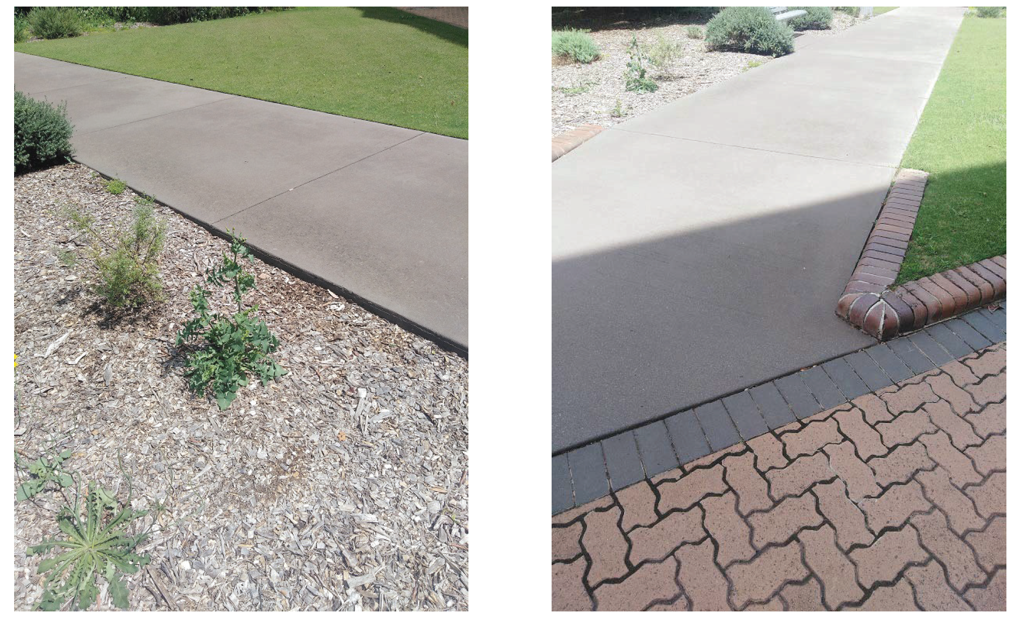
The Terrain Surface dataset, as presented in Table 8, provides valuable insights into the distribution of images across different terrain classes within both training and testing subsets. This dataset encompasses four primary terrain classes: Concrete, Tiles, Grass, and Rugged, each accompanied by a clear count of images in both training and testing sets. Notably, the dataset demonstrates a balanced distribution of samples among these classes, with each class having similar representation in both training and testing subsets. In total, the training set comprises 1,015 images, while the testing set contains 1,357 images. This balanced dataset serves as a valuable resource for developing and evaluating machine learning models tailored to terrain surface classification, ensuring fair and accurate assessments of model performance across diverse terrain types.

Table 8. Distribution of images for each class in the training and testing subsets of the Main Dataset.

Datasets	Training	Testing
Concrete	287	478
Grass	232	306
Rugged	230	357
Tiles	266	216
Total	1015	1357

In Table 9, a comprehensive performance evaluation of state-of-the-art (SOTA) approaches on the Terrain Surface dataset is presented. This evaluation compares these methods based on key metrics, including their F1 score (indicative of model accuracy), Floating Point Operations Per Second (FLOPS) specific to terrain surface computations, and the number of training parameters. The models examined encompass MobileNetV1, MobileNetV2, MobileNetV3, ShuffleNet, SqueezeNet, and TerraWAVE. Notably, TerraWAVE outshines the competition with the highest F1 score of

92.98 %

, remarkable computational efficiency with a mere

0.123

FLOPS, and a relatively modest

46, 960

training parameters, establishing its exceptional efficiency and effectiveness in terrain surface analysis. Conversely, MobileNetV2 exhibits the lowest F1 score at

86.65 %

, with moderate FLOPS of 625 and a larger parameter count at

2, 264, 389

. MobileNetV1 and ShuffleNet share similar FLOPS at 972, but ShuffleNet carries a higher parameter load of

4, 023, 865

. SqueezeNet achieves an F1 score of

91.66 %

with the lowest FLOPS at 531 and the smallest parameter count,

725, 073

, excluding TerraWAVE. All models were trained under identical conditions, highlighting the intricate trade-offs between model accuracy, computational efficiency, and complexity in terrain surface analysis.

8. Real-Time Validation

The online classification system has been designed to get surface information. This surface score will feed into the controller to maintain AGV in a predefined path. The whole learning process is based on an unsupervised method. The specific surface location in a particular image is provided to the controller for generating the control action for AGV. For achieving this, we have divided the image frame into two parts. It is obtained by vertically splitting the image frame. After that, the divided image frames feed into the model. The model will give an output surface score as well as image location in a particular scene.

Experiment I

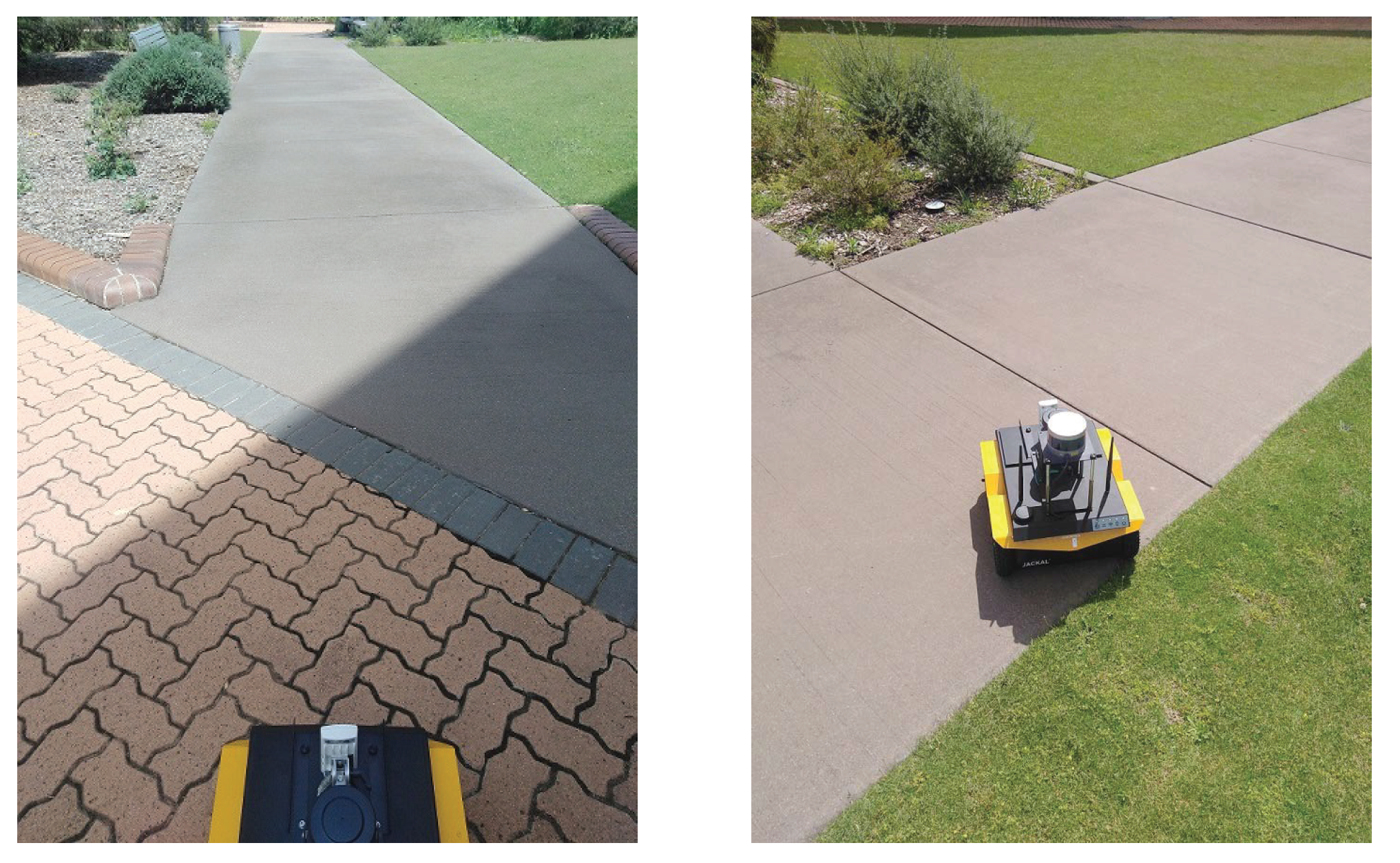
Outdoor experiments are conducted to show the effectiveness of the method on heterogeneous surfaces. Thus, more challenging experiments involving mixed terrains are performed. In order to improve the efficiency of AGV on outdoor terrains/surfaces and smooth traversing, the vision-based surface classification will assist the AGV in choosing its path on mixed surfaces [Figure 7].

The AGV’s traversable surfaces are classified using a camera and these surfaces are prioritized based on the vehicles control efforts while traversing. So the ground surfaces are classified as `concrete’, `grass’, `rugged’, and `tiles’. The best traversable surface is prioritised in the order of less controller effort i.e., [Concrete (more preferred), Tiles, Grass, Rugged (less preferred)]. The experiment is conducted on heterogeneous surfaces and illustrated in Figure 8.

Experiment II

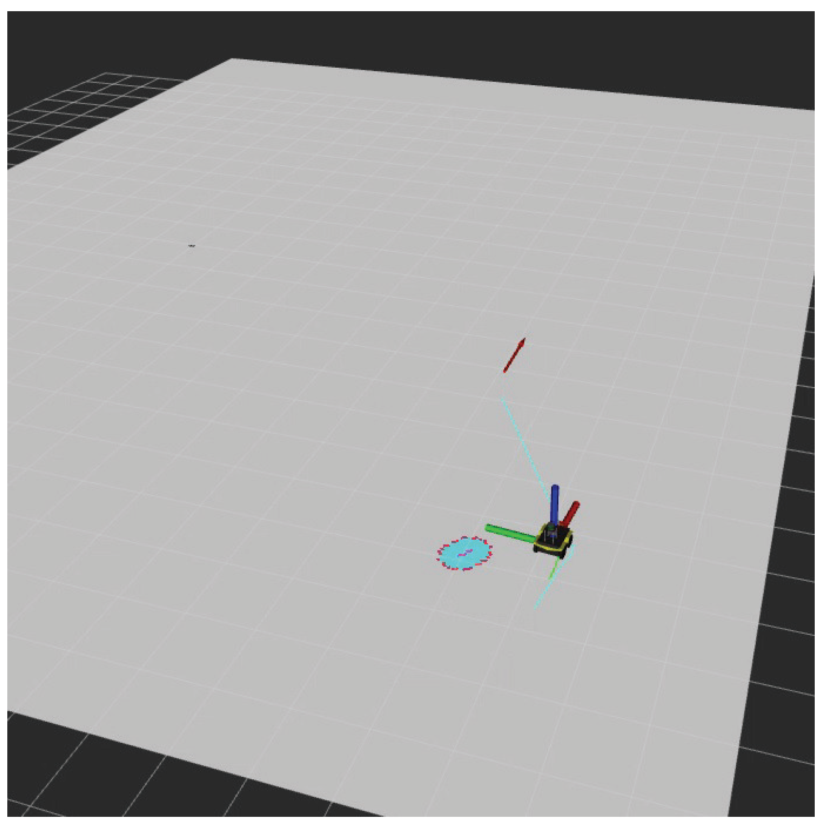
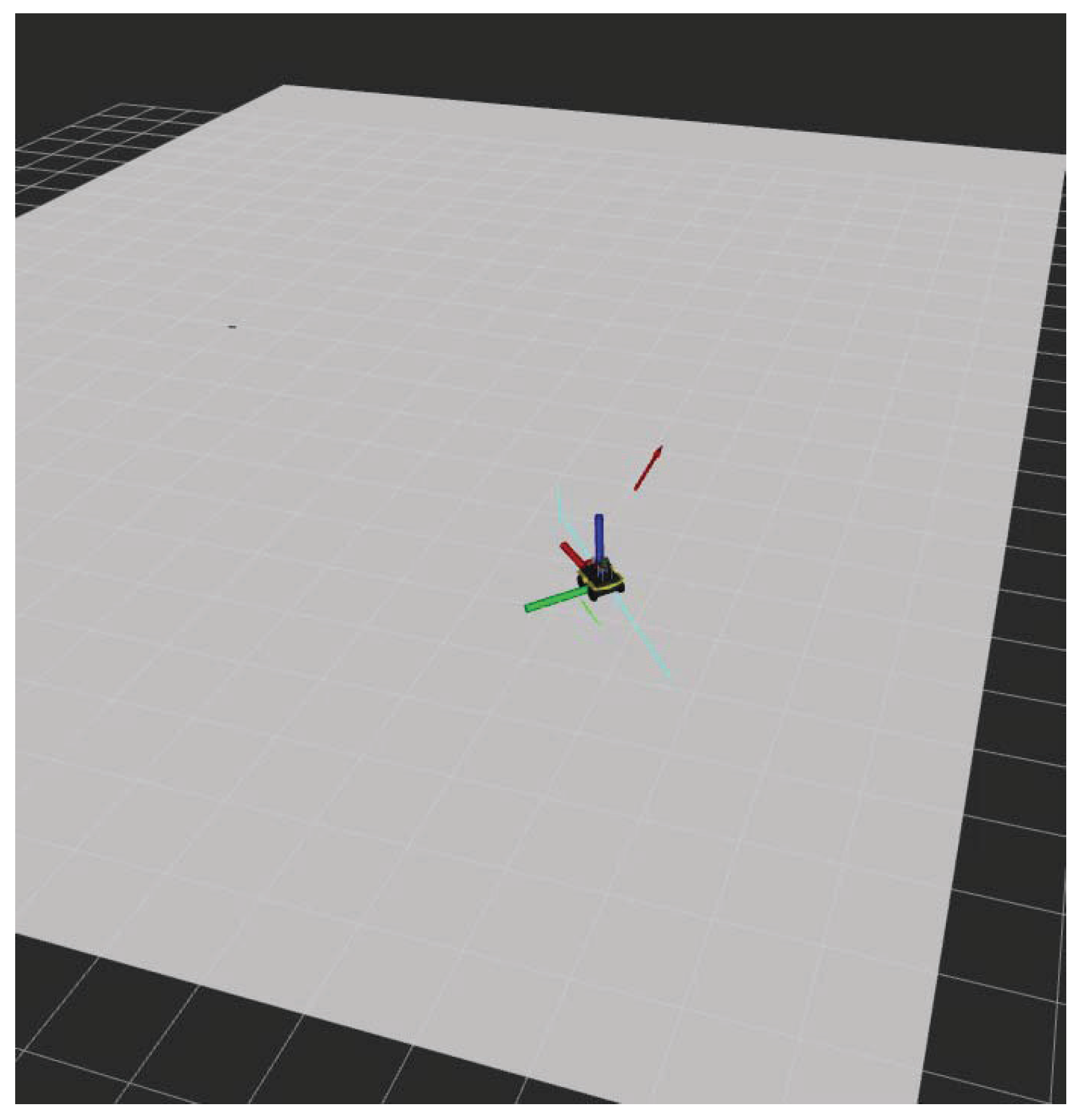
In this experiment II, surface classification is integrated as a part of Jackal’s path planning setup. The figure below shows the screenshots of the experiment visualised in RVIZ. In the experiment, AGV can successfully differentiate the surfaces and it is able to choose the Concrete surface over the Grass surface.

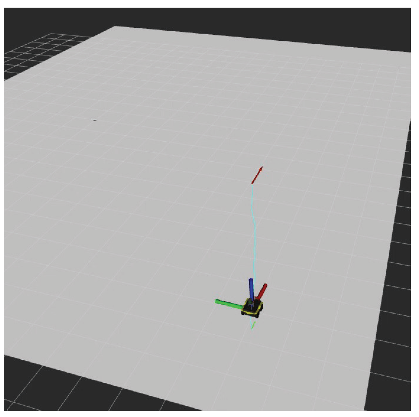
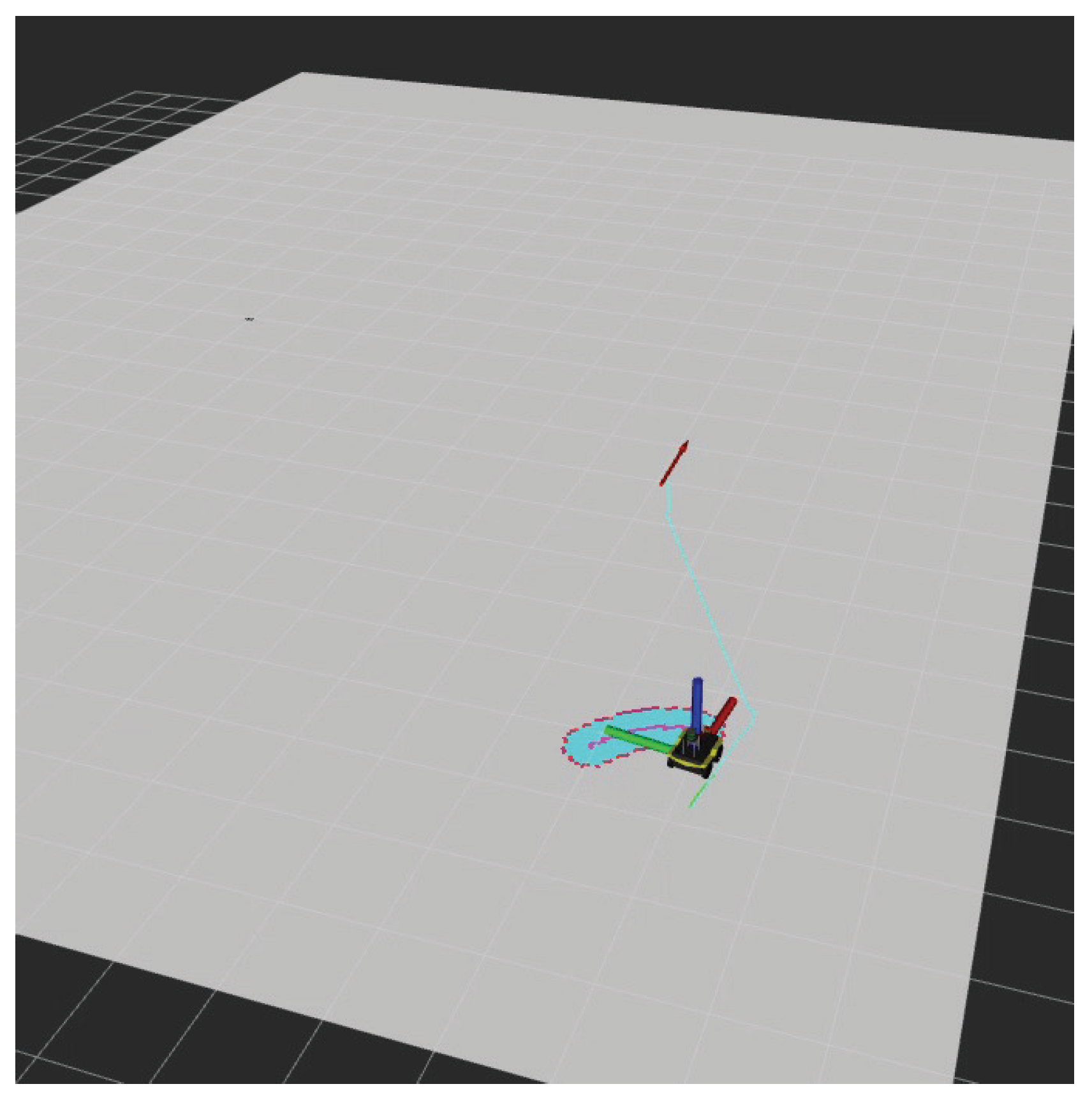
AGV is set to travel from an initial position in Figure 9 to a goal position in Figure 12. The AGV traverses its initially planned path by perceiving its immediate surfaces at regular intervals while traversing. The real-time experimental videos are in the link below:

https://www.dropbox.com/s/7ucc2qrqfcjdvup/Experiment%20VII%201%20.mp4?dl=0

https://www.dropbox.com/s/78ww9tiod3wa39y/Experiment%20VII%202%20.mp4?dl=0

Figure 9. Initial planned path.

Figure 10. Replanned path to avoid the Grass surface.

Figure 11. Following the replanned path.

Figure 12. Reached the Goal.

9. Conclusions

The paper introduces a novel lightweight surface classification model for enhancing the search and rescue capabilities of agile mobile robots. By integrating navigation, real-time data, and adaptive terrain perception, a system is developed to adapt rapidly and make informed decisions in dynamic environments.

This paper presents a real-time surface classification model employing Fourier gating mechanism-based atrous Convolutional Neural Network (CNN). Then, the terrain classification for the vehicle`s path is used to increase the AGV`s performance on different outdoor terrains. The AGV can able to perceive and understand its environment continuously. This perception allows it to adapt to different terrains and obstacles seamlessly. A vision-based terrain perception strategy with a TerraWave Classifier (

Q_{β}

) is employed to identify the ground surfaces. To further evaluate the controller, the AGV is tested on different surfaces. For this, the real-time camera data is used to identify different terrains and the results of the experiments demonstrated that the AGV successfully navigated through different terrains and performed effectively in real-time.

Author Contributions

Sobers Francis: Data curation, Formal analysis,Methodology, Project administration, Resources, Software, Visualization Design, Methodology, Investigation, Writing - original draft. Tanmoy Dam: Data curation, Formal analysis, Methodology, Project administration, Resources, Software, Visualization Design, Methodology, Investigation, Writing - original draft. Sreenatha Anavatti: Review editing, Supervision, Funding acquisition, Validation, Writing - review & editing. Matthew A Garratt: Review editing, Supervision, Funding acquisition, Validation, Writing - review & editing.

Abbreviations

The following abbreviations are used in this manuscript:

CNN	Convolutional Neural Network
AGV	Autonomous Ground Vehicle
ROS	Robot Operating System

References

Guan, T.; He, Z.; Song, R.; Manocha, D.; Zhang, L. TNS: Terrain Traversability Mapping and Navigation System for Autonomous Excavators.
Chen, C.S.; Lin, C.J.; Lai, C.C.; Lin, S.Y. Velocity Estimation and Cost Map Generation for Dynamic Obstacle Avoidance of ROS Based AMR. Machines 2022, 10, 501. [Google Scholar] [CrossRef]
Walas, K. Terrain classification and negotiation with a walking robot. Journal of Intelligent & Robotic Systems 2015, 78, 401–423. [Google Scholar]
Islam, F.; Nabi, M.; Ball, J.E. Off-road detection analysis for autonomous ground vehicles: a review. Sensors 2022, 22, 8463. [Google Scholar] [CrossRef] [PubMed]
Sánchez, M.; Morales, J.; Martínez, J.L. Reinforcement and curriculum learning for off-road navigation of an UGV with a 3D LiDAR. Sensors 2023, 23, 3239. [Google Scholar] [CrossRef] [PubMed]
Dam, T.; Ferdaus, M.M.; Pratama, M.; Anavatti, S.G.; Jayavelu, S.; Abbass, H. Latent preserving generative adversarial network for imbalance classification. 2022 IEEE International Conference on Image Processing (ICIP). IEEE, 2022, pp. 3712–3716.
Dam, T. Developing Generative Adversarial Networks for Classification and Clustering: Overcoming Class Imbalance and Catastrophic Forgetting. PhD thesis, UNSW Sydney, 2022.
Dwaracherla, V.; Thakar, S.; Vachhani, L.; Gupta, A.; Yadav, A.; Modi, S. Motion planning for point-to-point navigation of spherical robot using position feedback. IEEE/ASME Transactions on Mechatronics 2019, 24, 2416–2426. [Google Scholar] [CrossRef]
Chai, J.; Kayacan, E. Nonlinear Simulation and Performance Characterisation of an Adaptive Model Predictive Control Method for Booster Separation and Re-Entry. Electronics 2023, 12, 1488. [Google Scholar] [CrossRef]
Roucek, T.; Pecka, M.; Cızek, P.; Petrıcek, T.; Bayer, J.; Šalansky, V.; Azayev, T.; Hert, D.; Petrlık, M.; Báca, T.; others. System for multi-robotic exploration of underground environments CTU-CRAS-NORLAB in the DARPA Subterranean Challenge. arXiv preprint arXiv:2110.05911 2021.
Liu, Y.; Liu, G. Track–Stair Interaction Analysis and Online Tipover Prediction for a Self-Reconfigurable Tracked Mobile Robot Climbing Stairs. IEEE/ASME Transactions On Mechatronics 2009, 14, 528–538. [Google Scholar]
Hong, S.; Choi, J.S.; Kim, H.W.; Won, M.C.; Shin, S.C.; Rhee, J.S.; Park, H.u. A path tracking control algorithm for underwater mining vehicles. Journal of mechanical science and technology 2009, 23, 2030–2037. [Google Scholar] [CrossRef]
Lalonde, J.F.; Vandapel, N.; Huber, D.F.; Hebert, M. Natural terrain classification using three-dimensional ladar data for ground robot mobility. Journal of field robotics 2006, 23, 839–861. [Google Scholar] [CrossRef]
Wu, Y.; Lv, W.; Li, Z.; Chang, J.; Li, X.; Liu, S. Unsupervised domain adaptation for vibration-based robotic ground classification in dynamic environments. Mechanical Systems and Signal Processing 2022, 169, 108648. [Google Scholar] [CrossRef]
Papadakis, P. Terrain traversability analysis methods for unmanned ground vehicles: A survey. Engineering Applications of Artificial Intelligence 2013, 26, 1373–1385. [Google Scholar] [CrossRef]
Brooks, C.A.; Iagnemma, K. Self-supervised terrain classification for planetary surface exploration rovers. Journal of Field Robotics 2012, 29, 445–468. [Google Scholar] [CrossRef]
Dam, T.; Deb, A.K. A clustering algorithm based TS fuzzy model for tracking dynamical system data. Journal of the Franklin Institute 2017, 354, 5617–5645. [Google Scholar] [CrossRef]
Lee, G.Y.; Dam, T.; Ferdaus, M.M.; Poenar, D.P.; Duong, V.N. WATT-EffNet: A Lightweight and Accurate Model for Classifying Aerial Disaster Images. IEEE Geoscience and Remote Sensing Letters 2023. [Google Scholar] [CrossRef]
Martinez-Martin, E.; Cazorla, M.; Orts-Escolano, S. Machine learning techniques for assistive robotics, 2020.
Guan, T.; Song, R.; Ye, Z.; Zhang, L. Vinet: Visual and inertial-based terrain classification and adaptive navigation over unknown terrain. 2023 IEEE international conference on robotics and automation (ICRA). IEEE, 2023, pp. 4106–4112.
Wong, J.Y. Terramechanics and off-road vehicle engineering: terrain behaviour, off-road vehicle performance and design; Butterworth-heinemann, 2009.
Wong, J.Y. Theory of ground vehicles; John Wiley & Sons, 2022.
Liu, Z.; Guo, J.; Ding, L.; Gao, H.; Guo, T.; Deng, Z. Online estimation of terrain parameters and resistance force based on equivalent sinkage for planetary rovers in longitudinal skid. Mechanical systems and signal processing 2019, 119, 39–54. [Google Scholar] [CrossRef]
Dam, T.; Anavatti, S.G.; Abbass, H.A. Improving ClusterGAN Using Self-AugmentedInformation Maximization of Disentangling LatentSpaces. arXiv preprint arXiv:2107.12706 2021.
Dam, T.; Anavatti, S.G.; Abbass, H.A. Mixture of spectral generative adversarial networks for imbalanced hyperspectral image classification. IEEE Geoscience and Remote Sensing Letters 2020, 19, 1–5. [Google Scholar] [CrossRef]
Qin, Y.; Xiang, C.; Wang, Z.; Dong, M. Road excitation classification for semi-active suspension system based on system response. Journal of vibration and control 2018, 24, 2732–2748. [Google Scholar] [CrossRef]
Wei, Y.; Wei, W.; Zhang, Y. EfferDeepNet: An Efficient Semantic Segmentation Method for Outdoor Terrain. Machines 2023, 11, 256. [Google Scholar] [CrossRef]
Mei, M.; Chang, J.; Li, Y.; Li, Z.; Li, X.; Lv, W. Comparative study of different methods in vibration-based terrain classification for wheeled robots with shock absorbers. Sensors 2019, 19, 1137. [Google Scholar] [CrossRef]
Howard, A.G.; Zhu, M.; Chen, B.; Kalenichenko, D.; Wang, W.; Weyand, T.; Andreetto, M.; Adam, H. Mobilenets: Efficient convolutional neural networks for mobile vision applications. arXiv preprint arXiv:1704.04861 2017. arXiv:1704.04861 2017.
Sandler, M.; Howard, A.; Zhu, M.; Zhmoginov, A.; Chen, L.C. Mobilenetv2: Inverted residuals and linear bottlenecks. Proceedings of the IEEE conference on computer vision and pattern recognition, 2018, pp. 4510–4520.
Howard, A.; Sandler, M.; Chu, G.; Chen, L.C.; Chen, B.; Tan, M.; Wang, W.; Zhu, Y.; Pang, R.; Vasudevan, V.; others. Searching for mobilenetv3. Proceedings of the IEEE/CVF international conference on computer vision, 2019, pp. 1314–1324.
Iandola, F.; Han, S.; Moskewicz, M.; Ashraf, K.; Dally, W.; Keutzer, K. SqueezeNet: AlexNet-level accuracy with 50× fewer parameters and< 0.5 MB model size. arXiv 2016. arXiv preprint arXiv:1602.07360.
Ma, N.; Zhang, X.; Zheng, H.T.; Sun, J. Shufflenet v2: Practical guidelines for efficient cnn architecture design. Proceedings of the European conference on computer vision (ECCV), 2018, pp. 116–131.
Tan, M.; Le, Q. Efficientnet: Rethinking model scaling for convolutional neural networks. International conference on machine learning. PMLR, 2019, pp. 6105–6114.
Zuo, X.; Zhang, M.; Chen, Y.; Liu, Y.; Huang, G.; Li, M. Visual-Inertial Localization for Skid-Steering Robots with Kinematic Constraints. CoRR 2019, abs/1911.05787, [1911.05787].
West, A.; Wright, T.; Tsitsimpelis, I.; Groves, K.; Joyce, M.J.; Lennox, B. Real-time avoidance of ionising radiation using layered costmaps for mobile robots. Frontiers in Robotics and AI 2022, p. 61.
Chen, L.C.; Zhu, Y.; Papandreou, G.; Schroff, F.; Adam, H. Encoder-decoder with atrous separable convolution for semantic image segmentation. Proceedings of the European conference on computer vision (ECCV), 2018, pp. 801–818.
Joshi, R.; Gg, L.P.; Faqeerzada, M.A.; Bhattacharya, T.; Kim, M.S.; Baek, I.; Cho, B.K. Deep Learning-Based Quantitative Assessment of Melamine and Cyanuric Acid in Pet Food Using Fourier Transform Infrared Spectroscopy. Sensors 2023, 23, 5020. [Google Scholar] [CrossRef]
Moreland, K.; Angel, E. The FFT on a GPU. Proceedings of the ACM SIGGRAPH/EUROGRAPHICS conference on Graphics hardware, 2003, pp. 112–119.
Francis, S.L.X.; Anavatti, S.G.; Garratt, M. Real-time path planning module for autonomous vehicles in cluttered environment using a 3D camera. International Journal of Vehicle Autonomous Systems 2018, 14, 40–61. [Google Scholar] [CrossRef]

Figure 1. Jackal with RGB Camera [Autonomous Lab @ UNSW Canberra].

Figure 2. AXIS Companion Cube L.

Figure 3. ROS Navigation Stack with Surface Classification Node.

Figure 7. Mixed Terrains/surfaces.

Figure 8. Experiments VI: Jackal AGV chooses its best path.

Table 9. Performance evaluation of various SOTA approaches on Terrain Surface dataset.

Methods	F1 (%) (↑)	FLOPS (↓)	# Parameters (↓)
MobileNetV1	91.37	972	3,233,861
MobileNetV2	86.65	625	2,264,389
MobileNetV3	89.32	112	1,535,093
ShuffleNet	91.29	972	4,023,865
SqueezeNet	91.66	531	725,073
TerraWave	92.98	0.123	46960

All models are trained on the same environment.

Disclaimer/Publisher’s Note: The statements, opinions and data contained in all publications are solely those of the individual author(s) and contributor(s) and not of MDPI and/or the editor(s). MDPI and/or the editor(s) disclaim responsibility for any injury to people or property resulting from any ideas, methods, instructions or products referred to in the content.

© 2023 by the authors. Licensee MDPI, Basel, Switzerland. This article is an open access article distributed under the terms and conditions of the Creative Commons Attribution (CC BY) license (http://creativecommons.org/licenses/by/4.0/).

Copyright: This open access article is published under a Creative Commons CC BY 4.0 license, which permit the free download, distribution, and reuse, provided that the author and preprint are cited in any reuse.

MDPI Initiatives

Important Links

Choose an area of interest and we will send you notifications of new preprints at your preferred frequency.

Disclaimer